Improved MRO Inventory Management System in Oil and Gas Company: Increased Service Level and Reduced Average Inventory Investment

Abstract

This study proposes a methodology for the oil and gas businesses to keep their production plant productive with a minimum investment in carrying maintenance, repair, and operating inventory planning. The goal is to assist the exploration and production companies in minimizing the investment in keeping maintenance, repair, and operating (MRO) inventory for improving production plant uptime. The MRO inventory is the most expensive asset and it requires substantial investment. It helps in keeping the oil and gas production plant productive by performing planned and unplanned maintenance activities. A (Q, r) model with a stock-out and backorder cost approach is combined with a continuous inventory review policy for the analysis of class A items of oil and gas production plant MRO inventory. The class A items are identified through popular ABC analysis based on annual dollar volume. The demand for the inventory is modeled through Poisson distribution with consideration of constant lead time. The (Q, r) model in both stock-out cost and backorder cost approaches assigned higher order frequency and lower service level to low annual demand and highly expensive items. The stock-out cost approach shows an 8.88% increase in the average service level and a 56.9% decrease in the company average inventory investment. The backorder cost approach results in a 7.77% increase in average service level and a 57% decrease in average inventory investment in contrast to the company’s existing inventory management system. The results have a direct impact on increasing plant uptime and productivity and reducing company maintenance cost through properly managing maintenance stock. The analysis is carried out on the oil and gas production plant’s MRO inventory data, but it can be applied to other companies’ inventory data as well. All the results reflected in this research are based on the inventory ordering policy of two orders per year. The inventory ordering frequency per year may be other than two orders per year depending on the type of organization.

1. Introduction

The maintenance, repair, and operating (MRO) inventory plays an important role in keeping the plant productive and reducing the downtime. In the oil and gas industry, production is highly dependable on the availability of a productive machine. In a contrary situation, companies use MRO inventory to reduce shut down and maintenance costs. In the spare parts industry, service is related to the availability of machines being supported. As the cost of Exploration and Production (E&P) of materials from earth decreases, the margin of the profit increases. One of the main sources of production cost is the maintenance cost which consumes spare parts, especially in the energy and transportation industries, holding spare parts for maintenance requires huge capital investment. Therefore, the management schedules both plant maintenance and spare parts in the warehouse in order to reduce production costs [1,2].

The most important decision in the oil and gas business is the decision of the spare parts inventory. Spare parts inventory of drilling and production are very expensive and difficult to manage as compared to the raw materials’ inventory which is demand-dependent and their managerial improvements can easily be achieved through better master production scheduling (MPS) in manufacturing industries [3]. Therefore, the oil and gas business focuses highly on managing spare parts inventory. Additionally, in the case of the plant’s shut down for at least five minutes due to the non-availability of emergency repair parts, it will cost the oil and gas companies massively in comparison with other discrete manufacturing industries. Hence, managing spare parts in the oil and gas industry has a great importance [4].

Most of the oil and gas companies use different policies and strategies for the spare parts management in order to increase service level and parts availability with minimum inventory investment. Some companies use a continuous review policy and others use a periodic review policy for checking inventory status for replenishment purposes. To determine the ordering quantity, Economic Order Quantity model (EOQ) is used more often, and for defining inventory maximum l and minimum level (Q, r), the Min–Max approach is used. The spare parts inventory management is a special case due to its characteristics of slow-moving and erratic demands. To model the erratic demand, researchers recommend Poisson distribution [5,6,7,8].

The raw materials, finished goods, and work-in-process (WIP) inventory are often kept in the manufacturing environment, due to which its consumption is known. Hence, there is less uncertainty in managing and forecasting their demand. In contrast, the MRO inventory has irregular demand due to which forecasting its demand is a difficult task compared to the regular demand inventory [9] and therefore, it has great uncertainty because its consumption only depends only on maintenance phenomena which are unpredictable events. Hence, MRO inventory management is a great challenge for businesses with respect to reducing access inventory and increasing service level towards maintenance phenomena [10].

One of the main reasons for the spare parts demand irregularity is the supplier lead time variability [11] and this demand fluctuation can be reduced by age-based replacement of spare parts in plant maintenance [12,13]. The inventory and demand management of spare parts is more critical than the components used in the assembly of finished products, due to rapid technological innovations, time or responsiveness (because of the responsive product support process, 23% of spares become obsolete every year) and the demand for spare parts (which tends to show a lumpy pattern) [14]. One of the main sources of production cost is maintenance cost which consumes spare parts. However, particularly in the energy and transportation industries, holding spare parts for maintenance requires huge capital investment. Therefore, management schedules both plant maintenance and spare parts in the warehouse in order to reduce production costs [1].

Supply chain management (SCM) supports companies to better manage demand, carry the right amount of inventory, deal with uncertainty, keep costs to a minimum and meet customer demand by providing enough service level [15]. Inventory management is the collection of techniques, tools, and strategies to keep the right inventory, at the right time, at the right place, at the right cost, and in the right quantity. Thus, the demand forecast is critical in supply chain management [16,17,18]. Inventory management is not an easy task, as when its level is not managed properly, it disturbs the company supply chain in terms of low productivity (due to lack of inventory) and more investment (due to access inventory). Therefore, inventory control and management are the tradeoffs between investment and service level.

In material management, spare parts channel the focus of the researchers to a separate field of spare parts management (SPM) due to its primary role in reducing plant downtimes and achieving companies’ planned goals of production and meet market demands. The total cost associated with spare parts supply chain networks cannot be controlled only by traditional material management policies and models, but considering the warehouse location optimizing and policy integration is the leading path to total cost reduction [19,20]. In the inventory management system, one of the critical inventory levels controlling parameters regarding total cost reduction is the optimal ordering quantity (Q). For that, Harris developed the first economic ordering quantity model (EOQ) with assumptions of constant and known demand. However, in a real industrial scenario (spare parts system), the demand pattern is interrupted due to unexpected equipment breakdown, and researchers extend the Harris assumptions to cope with real-life situations [21]. The performance of the inventory management system is highly dependable on the quality of demand prediction. Traditionally for demand forecasting, the consumption history is used, but in the case of the spare parts inventory system, the equipment failure behavior and useful life of the equipment are a core factor to increase demand forecasting quality. The Remaining Useful Life (RUL) predictions of monitored components obtained from a Prognostics and Health Monitoring (PHM) system are used to predict future demands for non-repairable spare parts [22]. Willman’s bootstrap inventory management method with Laplace demand distribution also provides excellent results towards saving of spare parts inventory investment [23]. Jingyao Gu proved an iterative non-linear model with a demand shortages period of mean time to failure (MTF) effective in spare parts inventory cost reduction in the aviation industry [24]. Then, Sergio Afonso [25] proposed a spare parts management optimization model based on the genetic algorithm and the physical asset life cycle, which works on the principles of activity-based costing and helps the managers identify the optimal inventory management policy. The Weibull-based failure rate behaviors along the life cycle are considered to have a more realistic representation of the demand and more accurate computation of the logistics costs associated with the different types of spare parts [26]. Internet of Things (IoT) also reduces the inventory cost and improves the service level by real-time monitoring of the manufacturing process. It also helps in the traceability of the faulty equipment. The increased collaboration among the inventory suppliers also minimizes the bullwhip effect [27]. Due to the spare parts inventory demand uncertainty of the aviation industry, traditional demand forecasting models do not perform well. This happens due to the variation in demand time and quantity. Merve and Fahrettin developed a novel inventory model to forecast the quantity and reorder point for the spare parts inventory. The comparison with the traditional models shows better results. Because of this, the overall maintenance and operational cost of the aviation industry are reduced. A total of 630 spare-part items of the Turkish Airline were selected. The developed model by was applied for the Q-R estimation. Better results were achieved as compared to the traditional models [28]. For the critical manufacturing systems, a service contract with the equipment supplier is essential. This ensures increased system reliability and availability. Timely availability of the spare parts inventory by the supplier is critical to ensure the system performance. To cater to this need, a Bill of Material (BOM) is available with the supplier. The BOM helps suppliers in forecasting the spare parts inventory requirement. Because of the complexity of the systems, the BOM is usually not in line with the different machine configurations. This leads to the inaccurate spare parts inventory estimation. Stip and Houtum developed a method to solve this issue. With the implementation of the developed method in a semi-conductor industry, a service level of 95% is ensured [29]. The inventory items segmentation concept is used to model multi-echelon spare parts. As a result, an optimum inventory grouping solution is obtained. The model comprises a mixed-integer non-linear problem (MINLP) which is solved by a greedy heuristic. The proposed model also helps management to perform sensitivity analysis, test different real-time scenarios and implement the best-suited solution to the organization [30]. For the spare parts (Q,R) calculation, the expected orders during a specific time are calculated using Bayesian estimates. This has further improved the demand estimation accuracy [31]. The multi-echelon technique for the recoverable item control (METRIC) is a mathematical model in which the average spare part item demand is estimated using the Bayesian estimation process. The objective of the METRIC is to estimate the optimal values of the multi-item’s spare parts inventory in a warehouse, warranting minimum backordering and holding costs [32]. The discrete Weibull Distribution (WD) is used to predict the demand of the spare parts in a multi-item demand scenario. The WD is used in combination with the multi-echelon technique for the recoverable item control (METRIC). In the multi-item spare parts scenario, the stochastic nature of the demand is modeled. The developed model is applied to an industry as a case study considering 97 items. It is found that the combination of WD along with the METRIC yields better demand estimation for the multi-item spare parts. This helps in the operational sustainability of the plant and helps in reducing the maintenance costs [33]. The spare parts inventory demand forecast in METRIC is based on the Poisson Distribution. The demand forecast is further improved by Costantino (authors) by employing Zero-Inflated Poisson (ZIP) distribution. The novel ZIP-METRIC model is applied on 1739 spare parts items of an airline as a case study. The result indicates that the ZIP-METRIC outperforms the traditional METRIC in terms of spare parts demand estimation [34].

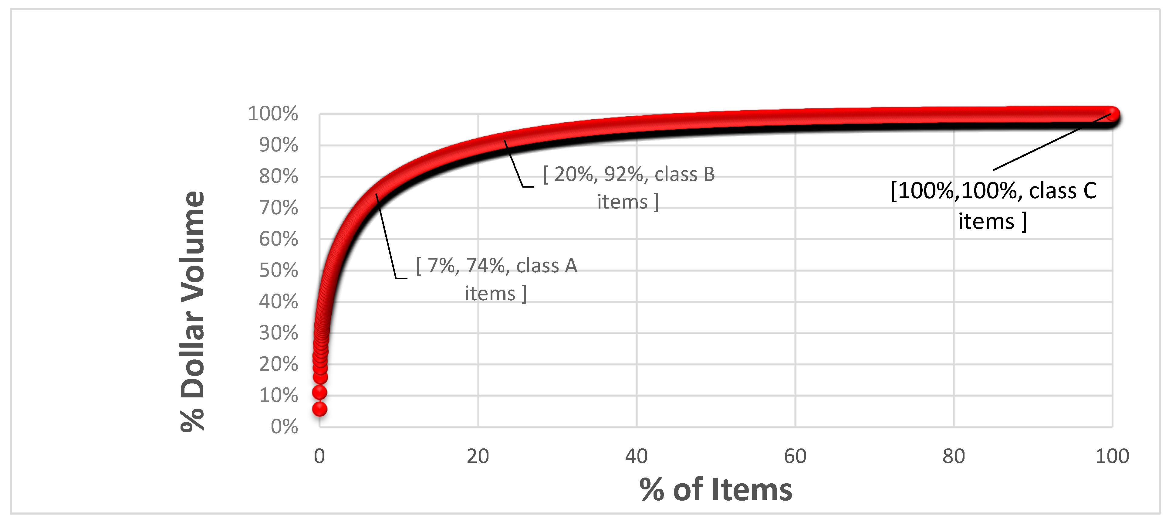
In this paper, the spare parts inventory of an oil and gas company is studied. A single storeroom inventory is focused that comprises drilling, production, and project inventory. In total, 4200 items of the storeroom are divided into three classes using ABC analysis. The ABC method is a popular method used in inventory management for the inventory classification in three different classes, i.e., A, B, and C. The class A items are usually in a lower quantity (about 20% of the product volume) but their inventory worth is much higher (about 80% of the total product worth). The class B items show worth of about 15% but their quantity is approximately 30% of the total inventory. The class C items are less expensive items (usually of the worth of about 5% of the total product worth) but their quantity is about 50%. Indonesia spare parts company used this technique for its inventory classification and as a result, increased its inventory turnover ratio and decreased its inventory cost [35]. Management of stock by accurate demand forecasting and stock classification is important for an organization to maximize profit and reduce cost [36]. The purpose of the ABC analysis in this research is:

• To find out the expensive spare parts based on annual dollar volume criteria;
• To keep its inventory in tight control;
• To reduce average inventory investment and,
• To increase spare parts providing service level to the production plant of an oil and gas company.

The classical ABC analysis (Annual Dollar Volume-Based Analysis) does not work properly in case of multi-criteria discrimination of all the potential parameters of the various items in the inventory. Therefore, in such a case, multi-criteria ABC classification is used which classifies inventory based on multiple factors consideration at a time. The existing criteria in the literature for the classification of spare parts inventory are: criticality, lead time, inventory cost, commonality, and the number of requests for an item per year, etc. [37].

The targeted company currently uses a Min–Max inventory control system with an inventory periodic review policy for the entire inventory while in this paper, the ABC analysis and (Q, r) model are used for the inventory controlling purpose with continuous reviewing of the stock level. This helps in the reduction of average inventory investment with a sufficient increase in service level. The (Q, r) model simply defines the two inventory controlling parameters which are Q (ordering quantity) and r (reorder point). Hence, the objective includes the provision of the optimum value of Q and r to oil and gas companies for each item in the MRO inventory warehouse, with minimum average inventory investment and an increase in the service level of order fill rate. The spare parts inventory management is challenging due to the unstable demand pattern. Therefore, the novelty of this work rests in estimating the optimum values of MRO inventory. A comprehensive framework for the estimation of optimum values is presented in the methodology section. The proposed approach is applied to real organizational data and the results are verified, validated and implemented. The same approach can be adopted by the other oil and gas E&P plants.

The remainder of the article is outlined as follows. In Section 2, the methodology is illustrated while results are explained and discussed in Section 3. In Section 4, some concluding remarks are presented.

2. Methodology

The management of spare parts is an essential part of the overall maintenance policy, which is a key determinant of the operational efficiency in a manufacturing system. In most of the plants, there are two types of maintenance activities performed. One is preventive maintenance which is the execution of planned activities and second is corrective maintenance which is the execution of unplanned activities for emergency repairs. The MRO used in preventive maintenance can be easily managed simply through Material Requirement Planning (MRP) logic, but the operational spare parts used in corrective maintenance cannot be managed through simple MRP logic. In spare parts management, the most important decisions are how much to order (Q) and when to order (r). Addressing both these decisions simultaneously is the focus of the (Q, r) model. Thus, to manage the operational spares, the (Q, r) model is a potential tool for identifying tradeoff between keeping less stock and providing high service to plant maintenance activities [38].

The research designed in this paper reflects the inventory controlling efficiency in terms of service level and backorder level. The company currently operated the inventory system on an average of 90% service level using the Min–Max method. The purpose of this research is to enhance the service level from 90% with a decrease in the average inventory investment. We used two approaches based on (Q, r) model which are the stock-out cost approach and the backorder cost approach. In the stock-out cost approach, each time cost is charged when the end-user demand cannot be filled from the available stock while in the case of the backorder cost approach, a penalty cost is considered which is proportional to the length of delay time. The cost parameters are calculated based on real data and through a specific equation as mentioned in the article to assist in the accurate analysis. The data are presented in

Table 1. Basic Data for (Q, r) model Parameters Calculation.

Part(j)	Dj (Units/Year)	Cj (USD/Unit)	Lj (Days)	θj (Units)	σj (Units)	Qj (Units)
1	108	704.74	90	26.63	5.16	71.971
2	105	669.47	20	5.75	2.40	72.809
3	40	41,680	90	9.86	3.14	5.695
4	93	487.76	20	5.10	2.26	80.278
5	55	559.12	97	14.62	3.82	57.662
6	53	597.63	29	4.21	2.05	54.749
7	28	33,588	93	7.13	2.67	5.308
8	30	826.01	62	5.10	2.26	35.037
9	38	1086.32	70	7.29	2.70	34.385
10	75	216.34	69	14.18	3.77	108.248

.

2.1. ABC Analysis

The data for analysis are collected from the database of a company for a single storeroom. The total number of items in the storeroom for which data are collected is 4200. It shows 7% class A items having 74% inventory worth, 13% class B items having 18% worth of inventory, and 80% class C items of 8% worth based on ABC analysis as shown in Figure 1. The spare parts classification carried out in this research is based on annual dollar volume in which the item consumption per year is multiplied by the unit price of the item and it is calculated on the basis of the percentage of annual dollar volume. Finally, the percentage of annual dollar volume is arranged in descending order. Then, we calculated the cumulative percentage of dollar volume which classifies the items into A, B, and C classes. Figure 1 shows the ABC classification of all the 4200 items based on annual dollar volume.

The focus of this research is on the slow-moving and big-ticket items which belong to class A items. From Figure 1, it is clear that class A inventory item has 7% quantity and 74% worth. Thus, in the reduction of the average inventory investment, class A items play a critical role due to their expensiveness and low volume. For further analysis, based on the (Q, r) model stock-out and backorder approach, a sample of ten items is selected from the class A items. Figure 2 shows the Pareto analysis of the sample of ten items of class A for further calculation of (Q, r) model, in order to define the optimum level of safety stock, reorder point, and order quantity to reduce company average inventory investment and enhance service level from the company current service level of 90%. According to Figure 2, the first three items need tighter inventory control and hence more attention will be needed to control their inventory level.

2.2. Data Collection

Table 2. Case data related to consumption, demand, cost and time of 10 class A items.

Item ID	Consumption in Year							Earliest Date of Issuance, Return, and Receiving	Average Annual Demand (Units)	Unit Cost (USD/Unit)	Lead Time (Days)
	2009	2010	2011	2012	2013	2014	2015		D	C	L
1	24	146	141	131	127	100	86	2009	108	704.74	90
2	10	35	63	64	79	239	251	2009	106	669.47	20
3	60	48	45	42	25	35	45	2010	40	41,680	90
4	0	33	76	114	108	138	90	2010	93	487.76	20
5	0	48	26	37	108	100	62	2009	54	559.12	97
6	0	45	25	36	80	136	51	2009	53	597.63	29
7	0	40	35	25	33	17	20	2010	28	33,588	93
8	14	33	35	25	20	35	48	2009	30	826.01	62
9	0	0	35	45	36	45	32	2011	39	1086.32	70
10	0	67	85	82	102	127	64	2009	75	216.34	69

shows the data collected from the company database for ten class A items which include annual consumption from the year 2009–2015, annual demand, per unit cost, and lead time in days. Based on these data, further (Q, r) model parameters are calculated and compared with the company’s existing model. The calculation steps of the parameters (Q, r) model are described below. The probability distribution for the modelling demand pattern used in this paper is Poisson, which the majority researchers recommend for modelling spare parts’ unpredictable demand. There are many methods for calculating the annual demand but here we just rely on the average annual demand because our aim is to compare the results of the (Q, r) model with the company’s existing model for the same calculated annual demand of the company. The average annual demand is calculated using the spreadsheet formula.

2.3. The (Q, r) Model

There are two approaches to penalize poor service. One approach is to charge a cost each time the demand cannot be filled from the stock (i.e., when stock-out occurs). The second approach is to charge a penalty that is proportional to the length of time an order waits to be filled (i.e., when backorder occurs). In this study, (Q, r) model is studied and its performance is analyzed in terms of average inventory investment, fill rate, and backorder level and the results are compared with the company’s existing model. The (Q, r) model parameters used are provided in

Table 3. (Q, r) Model parameters.

Symbol	Description
D	Expected demand per year (in units)
L	Replenishment lead time (in days)
Θ	Expected demand during the lead time (in units)
Σ	The standard deviation of demand during the lead time (in units)
A	Order cost per replenishment (in a dollar)
C	Unit purchase cost (in a dollar)
K	Cost per stockout (in a dollar)
b	Backorder cost (in dollar)
Q	Replenishment quantity, decision variable (in units)
R	Reorder point, decision variable (in units)
S	r − θ called safety stock (in units)
F	Order frequency per year
S	Fill rate service level (fraction of orders filled from stock)
B	The average number of backorders
I	Average on-hand inventory

and they are calculated using Equations (1)–(17) from the study of W. J. Hopp et al. [20].

The (Q, r) model is shown in Table 2, calculated based on real data using Equations (1)–(17) as mentioned in the article. The basic data for calculating the cost and other (Q, r) model parameters refer to Table 1.

The ordering quantity (Q) is the quantity that is ordered when the inventory reaches to replenishment level. The inventory ordering, holding and carrying costs at this quantity Q* becomes equal to:

$$Q^{*}=\sqrt{\frac{2AD}{H}}$$

(1)

where Q* is ordering quantity, A is ordering cost per replenishment, D is average annual demand, and H is holding cost per unit per year. In this paper, the holding cost is replaced by unit cost C because the focus in this research is reducing inventory investment. This cost consists of several components such as storage and space charges, taxes, purchase and assurance, and the cost of obsolete inventory due to technological change [39]. A number of researchers have developed the Economic Production Quantity (EPQ) model by considering different parameters, such as shortage, backorder, setup cost, deterioration, constant or linear or power form of the demand, rework, scrap, inspection, machine breakdown [40]. As a special case, EOQ value for the perishable goods is calculated by Wilson’s Model modification in order to bring agility to the supply chain and respond quickly to the changing market needs [41]. Unlike the earlier developed models, this model is unique as the oil and gas companies only purchase the spare parts from outside to keep the plant up.

The inventory reorder point is the point at which inventory is replenished by ordering quantity (Q*) when the inventory of the spare parts reaches to this point. In the case of spare parts with uncertain demands, the reorder point is calculated by considering the standard deviation of the spare parts’ annual consumption, as mentioned in Equation (2).

$$r=\theta +Z\sigma$$

(2)

where r is reorder point, θ is expected demand during the lead time in units, σ is the standard deviation of demand during the lead time in units and Z is the value calculated from the normal distribution table. To use Equation (2) from the normal demand version, the Poisson distribution will be approximated by normal with mean θ and standard deviation $\sigma =\sqrt{\theta }$.

2.4. Stock-Out Cost Approach (SCA)

In the case of SCA, the spare parts demand tends to follow a Poisson distribution, and it is calculated using the following ratio mentioned in Equation (3).

$$Z={\left[\frac{K{D}_j}{K{D}_j+h{Q}_j}\right]}^{-1}$$

(3)

where K is the cost per stock-out in dollars, h is cost per unit, D is annual average demand and Q is ordering quantity. Equation (4) is used to find the value of Z through a spreadsheet. Equation (3) calculates the Z value which is used for the reorder point of the stock-out cost approach.

$$Z=((NORM.S.INV(\Phi (Z))$$

(4)

where,

$$\Phi (Z)=\frac{KD}{K{D}_j+h{Q}_j}$$

(5)

The expected demand during lead time is represented by θ and is calculated using Equation (6).

$$\theta =\frac{DL}{365}$$

(6)

where D is average annual demand and L is the lead time in days.

Safety stock is the minimum level of inventory of a spare part that must be held in order to avoid any stock-out situation. When the safety stock for an inventory item increases, the probability of the stock-out decreases, and vice versa. Safety stock is calculated using Equation (7).

$$SS=r-\theta$$

(7)

where SS is the safety stock, r is the reorder point, and θ is the average demand during lead time.

In the case of the stock-out cost approach, the average inventory investment is calculated by the satisfaction of the service level and average annual order frequency constraints. The company is operated by order frequency of an average of two orders per year and a service level of 90%. This study aims to achieve a 98% service level for the same order frequency of an average of two orders per year and to reduce average inventory investment. However, from Figure 3 in Section 3, it is clear that for the same service level, when the order frequency increases, the inventory average investment decreases. Thus, the (Q, r) model feasibility with respect to the company’s existing model will be checked for at least the minimum ordering frequency of two orders per year. The formula of the (Q, r) model for the calculation of the average inventory investment is:

$$I(Q,r)=\left(\frac{Q_j}{2}+(r-\theta )+B(Q,r)\right)\times UnitCost$$

(8)

where Q is quantity per order, $\left(r-\theta \right)$ is safety stock and B(Q, r) is the backorder level at ordering quantity of Q and reorder point of r. The backorder level in Equation (8) is calculated using Equation (9).

$$B_i(Q_i,r_i)=\frac{\left(\beta (r)-\beta (r+Q)\right)}{Q}$$

(9)

where β is constant and its value is calculated at the point of r and r + Q for each type of spare parts in the inventory. Using a spreadsheet, β is calculated using equation [10].

$$\beta (r)=\frac{1}{2}\{{[[(r-\theta )}^2+r][1-G(r)]]-[\theta (r-\theta )P(r)]\}$$

(10)

where G(r) and P(r) are the spreadsheet function and can be input in Excel as: P(r) = (Poisson. Dist. (r, θ, False)) and G(r) = (Poisson. Dist. (r, θ, True)).

To satisfy the average order frequency constraint for finding average inventory investment in Equation (8), the result of Equation (11) must be equal to the average two orders per year.

$$F(A)=\frac{{\displaystyle \sum _{i=1}^n\frac{D_i}{Q_i}}}{N}$$

(11)

where N is the total number of items in the inventory. The frequency is calculated as a function of the annual ordering cost per replenishment A. If F(A) is less than two orders per year, the value of A will decrease, and vice versa. For the average order of two orders per year, this equation provides the ordering cost per replenishment of 16,900 dollars. Similarly, the service level constraints of 98% will be satisfied by implanting Equation (12) as a function of the stock-out cost k.

$$S(k)=\frac{{\displaystyle \sum _{j=1}^n{D}_j{S}_j(Q_j,r_j)}}{{\displaystyle \sum _{j=1}^n{D}_j}}$$

(12)

where S (Q, r) is the fill rate at the point of ordering a quantity of Q and reorder point of r for each type of spare part in the inventory. The value of k increases if the value of the S(k) is less than 98% and decreases if the value of the S(k) is greater than 98%. The value of k is noted when S(k) is equal to 98% and when noted, the value of k is 12,500 dollars for S(k) equal to 98%. The equation of S (Q, r) is given below.

$$S_i(Q_i,r_i)=1-\frac{\left(\beta (r)-\beta (r+Q\right)}{Q_i}$$

(13)

where β is the backorder level at reordering point and summation of reorder point and ordering quantity. To calculate this back-order level using a spreadsheet, Equation (14) is used in an excel sheet.

$$B(r)=\theta P(r)+(\theta -r)[1-G(r)]$$

(14)

where P(r) is equal to Poisson. Dist. (r, θ, False) and G(r) is equal to Poisson. Dist. (r, θ, True) is the spread of mass and density functions, respectively.

2.5. Backorder Cost Approach (BCA)

In BCA, the average inventory investment is calculated by satisfying the average order frequency constraints of two orders per year and an average backorder level of 0.4 units per year. The value of the backorder of 0.4 is taken from the stock-out model and it is to check the performance of both approaches for the same order frequency and the same backorder level.

In BCA, for the reorder point calculation, the Z value is calculated using Equation (14).

$$Z={\left[\frac{b_j}{b_j+h_j}\right]}^{-1}$$

(15)

where b is the back-ordering cost and h is the holding cost per year. To calculate this value using a spreadsheet, the following formula is used:

$$Z=((NORM.S.INV(\Phi (Z))$$

(16)

To achieve an average order frequency of two orders per year, the same stock-out coast approach of Equation (11) is used which gives ordering cost per replenishment of 16,900 dollars. Equation (16) is used to satisfy backorder level constraint of 0.4 units.

$$B(b)={\displaystyle \sum _{i=1}^n{B}_j\left(Q_j,r_j\right)}$$

(17)

where B (Q, r) is the backorder level and it is calculated through Equations (9) and (10). In Equation (17), the total backorder level is calculated as a function of back-ordering cost b. If the value of B(b) is less than 0.4, the value of b will decrease otherwise it will increase if the value of the B(b) is greater than 0.4 units of total backorder level. To obtain 0.4 units’ backorder level per year, Equation (17) gives the value of back-ordering cost b equals to 70,000 dollars. All the remaining formulas will be used as in previous stock-out cost approach formulas for service level and average inventory investment. The formulas for service level and average inventory investment in BCA will be the same as used in SCA.

3. Results, Discussion and Validation

The (Q, r) model is analyzed in this paper on a real dataset based on the SCA and BCA. The purpose of this model is to provide a satisfactory service level to the company with a minimum average inventory investment than the company’s existing policy. The following results are obtained from the (Q, r) model in comparison with the company existing Min–Max method:

The (Q, r) model defines the lower service level, minimum safety stock, and small ordering quantity in both stock-out (SCA) and backorder (BCA) cost approach for all those items in the inventory which are most expensive and their annual demand is minimum than the other items in the warehouse. Thus, the (Q, r) model is the best-suited model for defining inventory controlling parameters for slow-moving and expensive items.

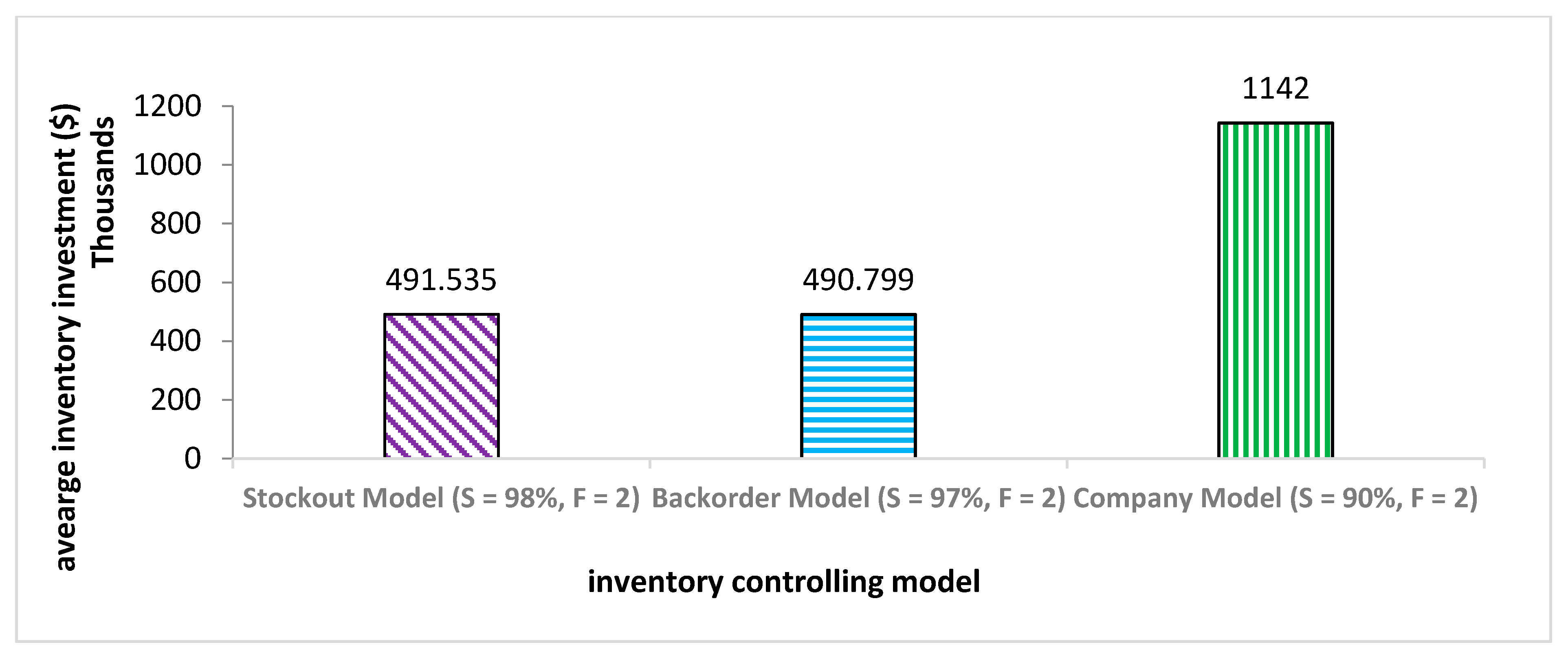
The (Q, r) model based on the stock-out cost approach and continuous inventory level review policy results in a total average inventory investment of USD 491,535 for the ten selected items of class A and an average service level of 98% for inventory ordering frequency of two orders per year. The company’s existing model has a total average inventory investment of USD 1,142,459 for the average annual inventory ordering frequency of two and a service level of 90% for each item in the inventory. The stock-out cost model reduced the inventory investment by 56.9% and increased the service level by 8.88% for the same ordering frequency of two orders per year. The main reason for this achievement of the stock-out cost model is allocating minimum safety stock and service level to low annual demand and expensive items in the inventory. On the other hand, the company Min–Max model based on periodic inventory level review policy defines 90% service level for each item (low demand and high demand) in the warehouse which results in high average inventory investment.

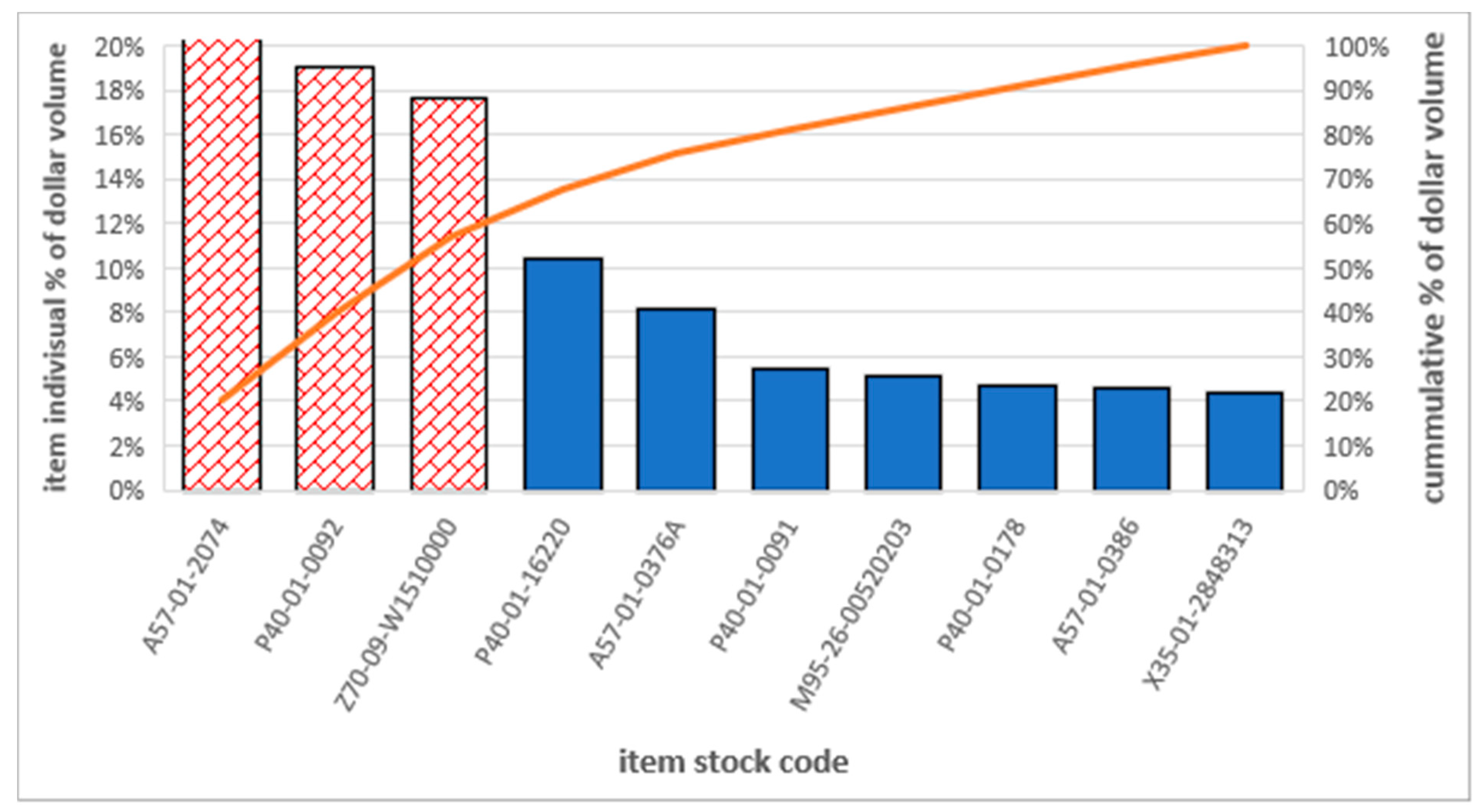
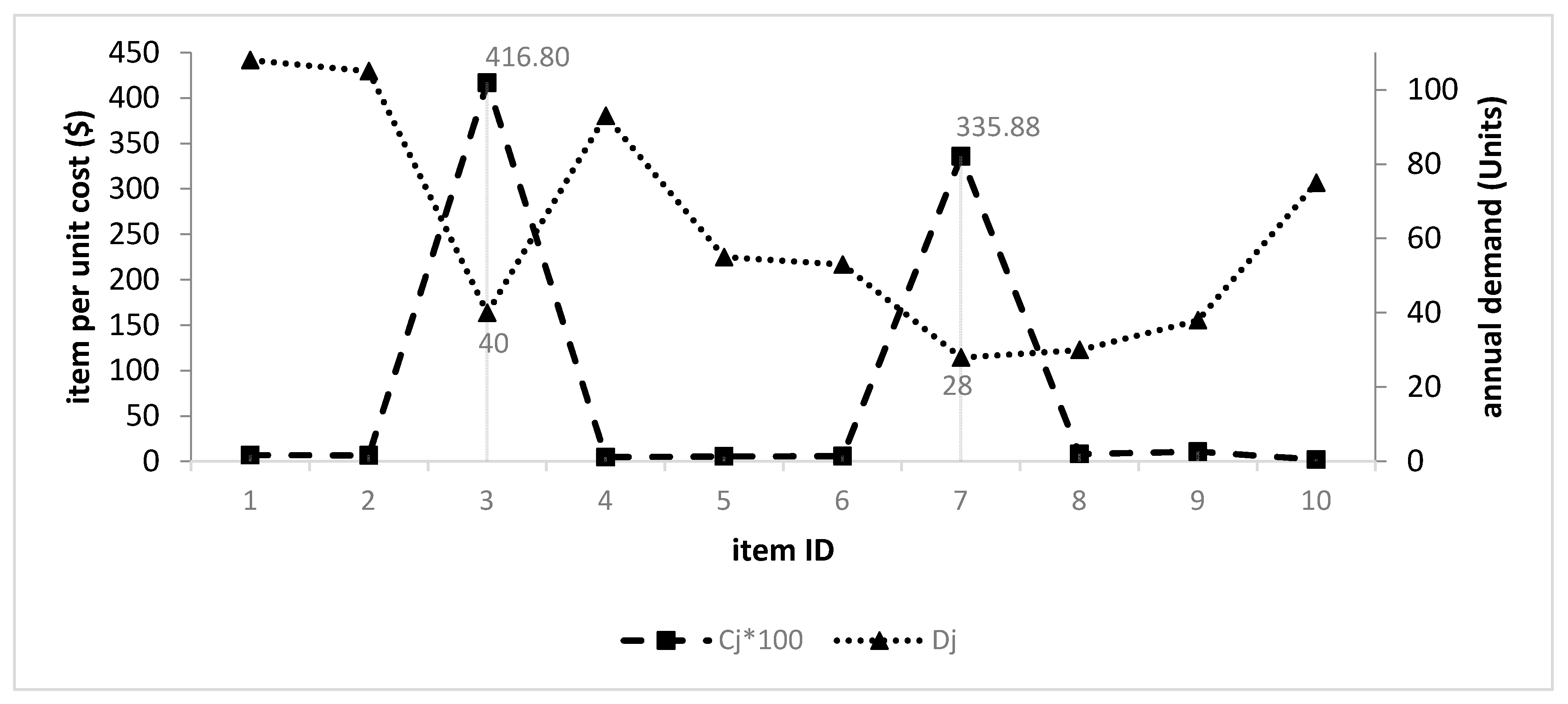
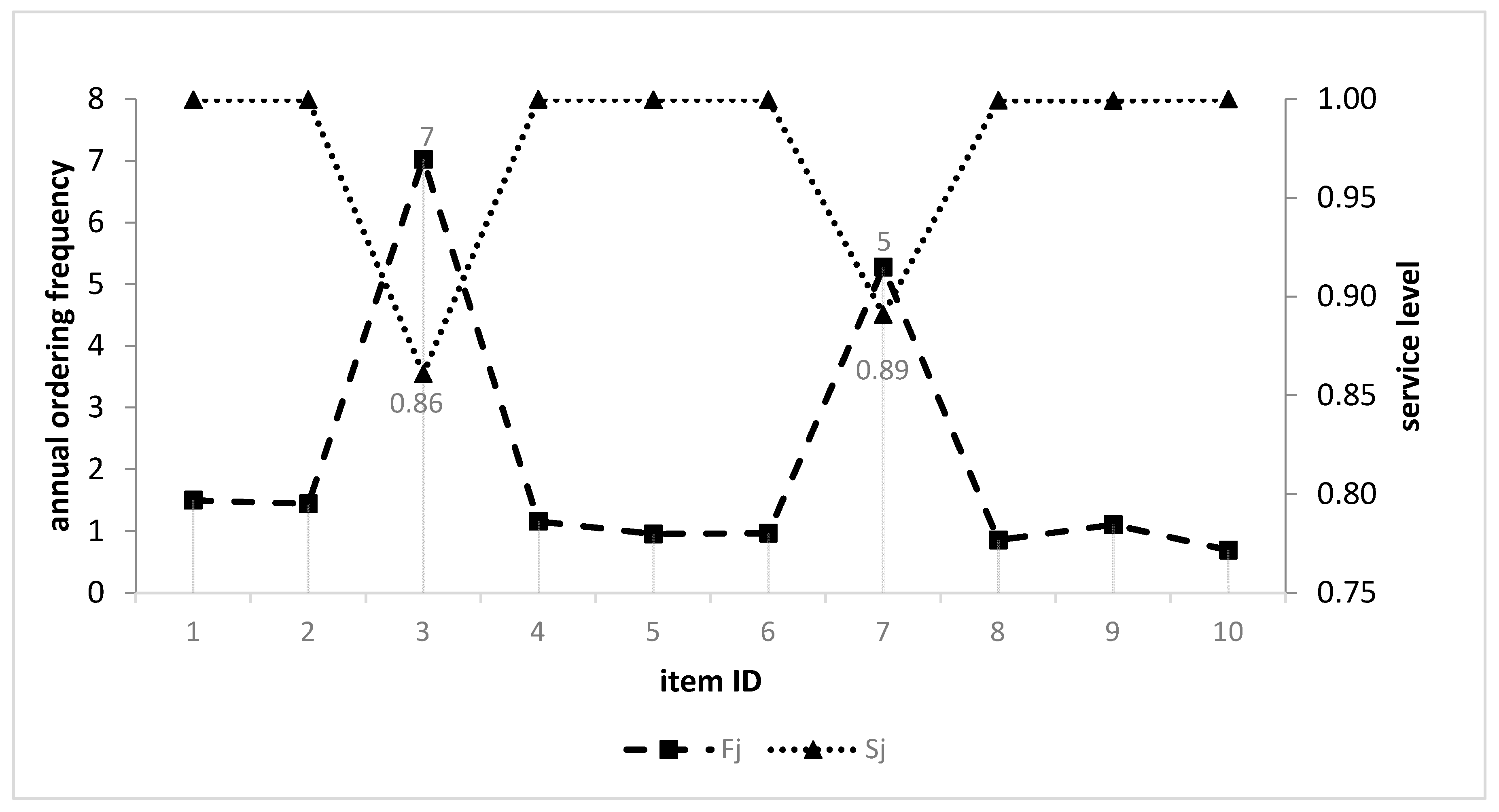
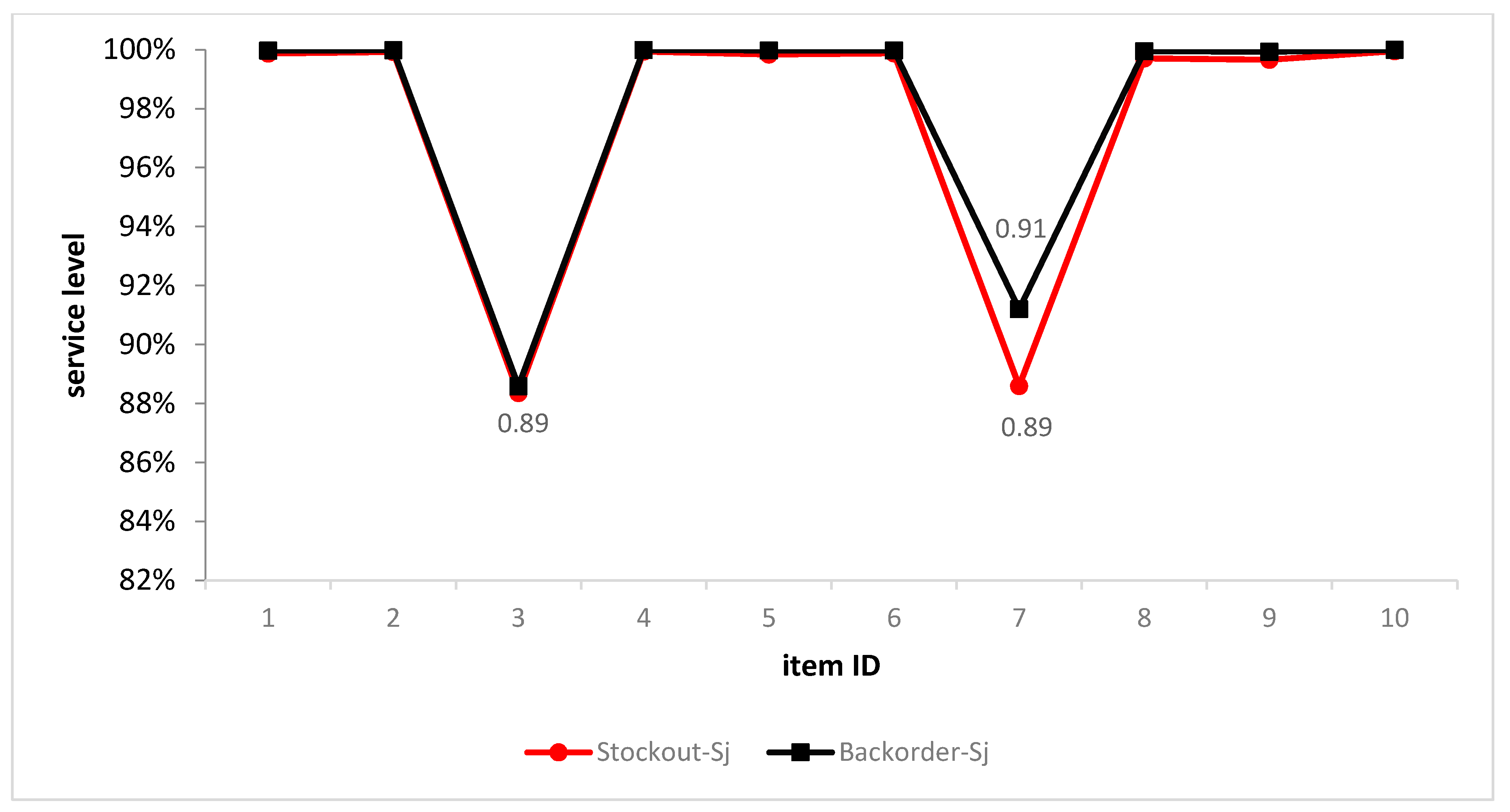
In Figure 4, the 3rd (Gate valve) and 7th items (Weighbridge) have a minimum annual demand of 40 units and 28 units, respectively. However, their per-unit cost is too high, at USD 41,680 and USD 33,588, respectively. The company Min–Max method allocate to both of these item 90% service level but the (Q, r) stock-out cost model allocates to these items low service levels of 88% and 89%, respectively. Due to this, the safety stock of these items is reduced, and hence, the average inventory investment is decreased. The remaining seven items are less expansive and they have high annual demand. Thus, the (Q, r) stock-out cost model allocates to each of these items a service level of 100% to achieve an average 98% service level instead of the company Min–Max method which allocates to these high annual demanded items a service level of 90%. Hence, in this way, the (Q, r) stock-out model gives an average service of 98% for an average annual order frequency of 2 with a reduction in average inventory investment of 56.9% which is a considerable financial saving.

The (Q, r) backorder cost model also assigned lower safety stock and low service level to the above mentioned expensive and low annual demand items. The average inventory investment acquired by the (Q, r) backorder cost model for the ten selected items is USD 490,799 and an average service level of 97% for an average order frequency of 2 orders per year. This is 57% less than the average inventory investment and the service level is 7.77% greater than the company’s existing Min–Max method.

The relation between average order frequency per year and average inventory investment is inversely proportional. When the average order frequency increases, the average inventory investment decreases and vice versa. However, when the service level increases, the average inventory investment also increases and vice versa. So, the (Q, r) model in both approaches (stock-out cost and backorder cost) assigned higher order frequency and lower service level to low annual demand and highly expensive Items.

In Figure 5, Fj shows order frequency and Sj shows the service level for each item. From Figure 4, items 3 and 7 are expensive items out of all ten selected items and they have a low annual demand. Hence, it is apparent that due to high unit cost and low annual demand, the (Q, r) model based on the stock-out cost approach assigned to these two items low service level of 86%, 89%, and order frequency of 7 and 5 orders per year respectively in achieving average service level of 97% and average order frequency of 2. Therefore, the advantage in low service is that when the service level is low, safety stock will be minimum, and hence, the average inventory investment will be minimum.

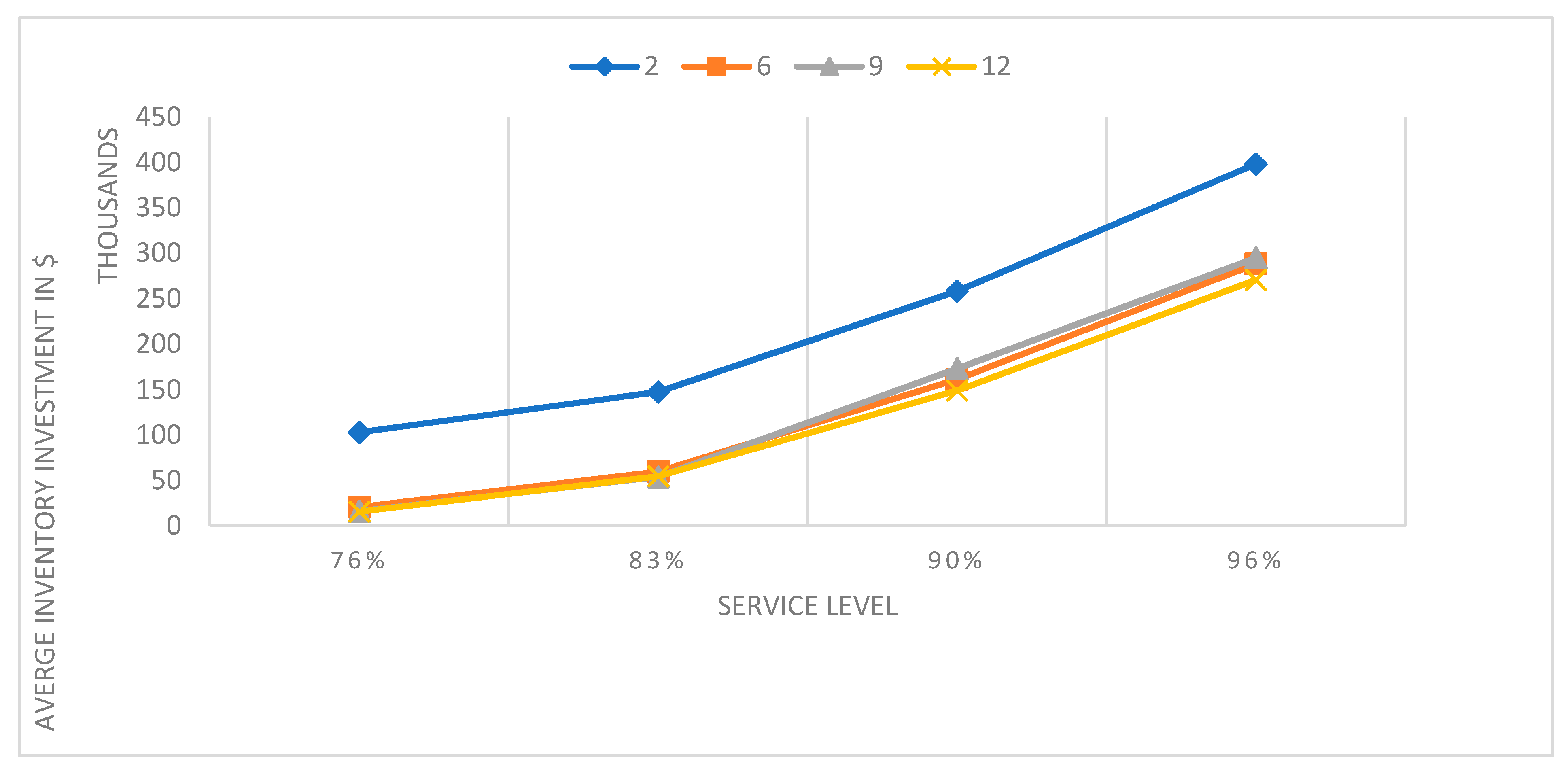
The high-order frequency allocation of (Q, r) model to items 3 and 7 implies that as the order frequency increases, the average inventory investment decreases. In Figure 3, the lines show the order frequency of 2, 6, 9, and 12, the x-axis shows service level, and the y-axis shows the average inventory investment. For the same service level, when the order frequency increases, the inventory average investment decreases.

Similarly, for the same order frequency, when the service level increases, the average inventory investment increases. Hence, the (Q, r) model attempts to reduce average inventory investment by allocating low service level and high order frequency to expensive and slow-moving items in the inventory.

The stock-out model results in USD 491,535 total average inventory investment for the ten selected items which is greater than the average investment of the backorder model as shown in Figure 6.

Hence, the backorder model performs better in reducing the average inventory investment. However, in the case of service level improvement, the stock-out model (SCA) performs better as it provides a greater service level of 98% to the inventory availability than the service level 97% of the backorder model. The stock-out cost model (SCA) controls the inventory by penalizing poor service each time when the end-user demand is not filled from the available stock (stock-out cost). The backorder cost model (BCA) manages the inventory by penalty cost (back-ordering cost) being considered proportional to the length of the time an end-user demand waits to be filled. A comparison of the results of the company model from Figure 6 shows failure in both the service and average inventory investment performance from either the stock-out model or backorder model. Thus, the results of the proposed (Q, r) models show improvement and justification for their use. In other words, from Figure 3, it is clear that there is an inverse relation between annual ordering frequency (F) and average inventory investment (I) for the same service level (S). For the same value of service level, when the value of F increases, the value of I decreases. In the future, if the company increases the value of F, the (Q, r) model will still be valid with respect to increasing service level and reducing average inventory investment. In the present research, on the critical lowest value of ordering frequency (F), the (Q, r) model shows improved results. Thus, for the highest value of F, a comparison with the company’s existing model will be needed in future analysis.

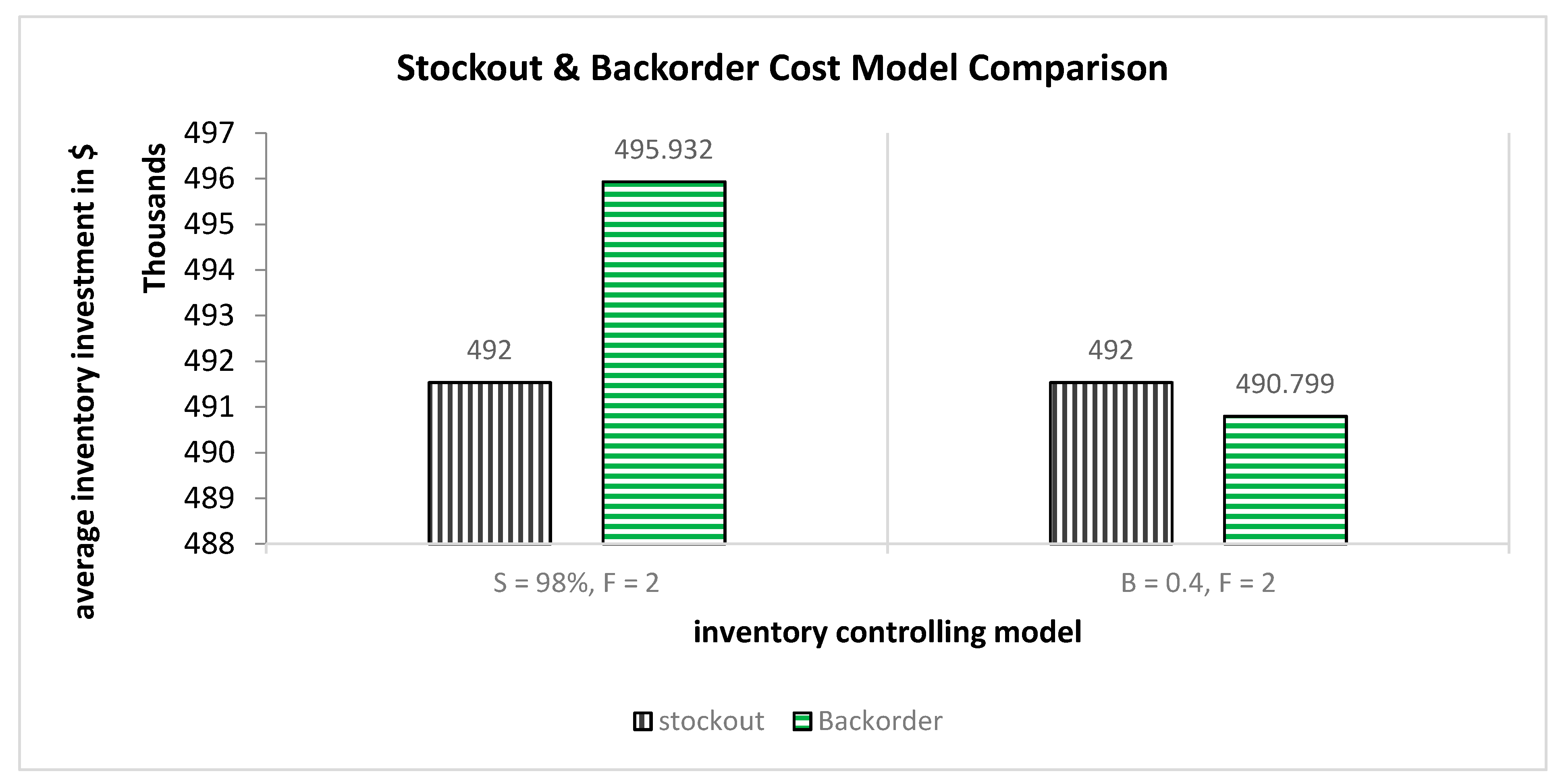
The comparison of the stock-out SCA model and backorder BCA model is graphically represented in Figure 7 with respect to average inventory investment for 98% service level, 0.4 back-ordering units, and order frequency of two orders per year. The service level shows the fraction of orders filled from the available stock. For example, if 100 orders are placed per year by the end-user, by a 98% service level, 98 orders will be fulfilled. The backorder level (0.4 units) is the critical measurement of the inventory management effectiveness and quality of service towards the customer. When the total backorder level increases, the customers wait more for the demand fulfilment than the lower backorder level per annum. Therefore, the more units at the backorder level, the greater the back-ordering cost will be. When the waiting time of the customer order fulfilment decreases, there must be an increase in the service level which is achieved by minimizing the average backorder level per year. As the focus in this research is to reduce average inventory investment with a satisfactory increase in service level, the backorder model is a tradeoff between backorder level and service level. According to Little’s law, the average backorder level of 0.4 units equals to an average waiting time of 6.3 h, which means that on average, any part out of the ten items will experience 6.3 h of delay due to the unavailability of on-time stock. The delay hours from the average backorder level is calculated by using Equation (18) (Little’s law).

$$W=\frac{B}{D}\times 8760\mathrm{h}$$

(18)

where B is the total backorder level, D is the sum of average demand per year and W is average waiting time of the customer request in hours (h) for a single inventory item.

Figure 7 shows that the backorder model performs better in achieving an average of 0.4 units of backorder level due to less inventory investment of USD 490,799 than the stock-out model. In the case of achieving an average service level of 98%, the stock-out cost model is the best option due to low inventory investment than the backorder model. Figure 8 shows the graph based on achieving an average of 0.4 units’ backorder level while Figure 9 shows the graph based on achieving an average service level of 98%.

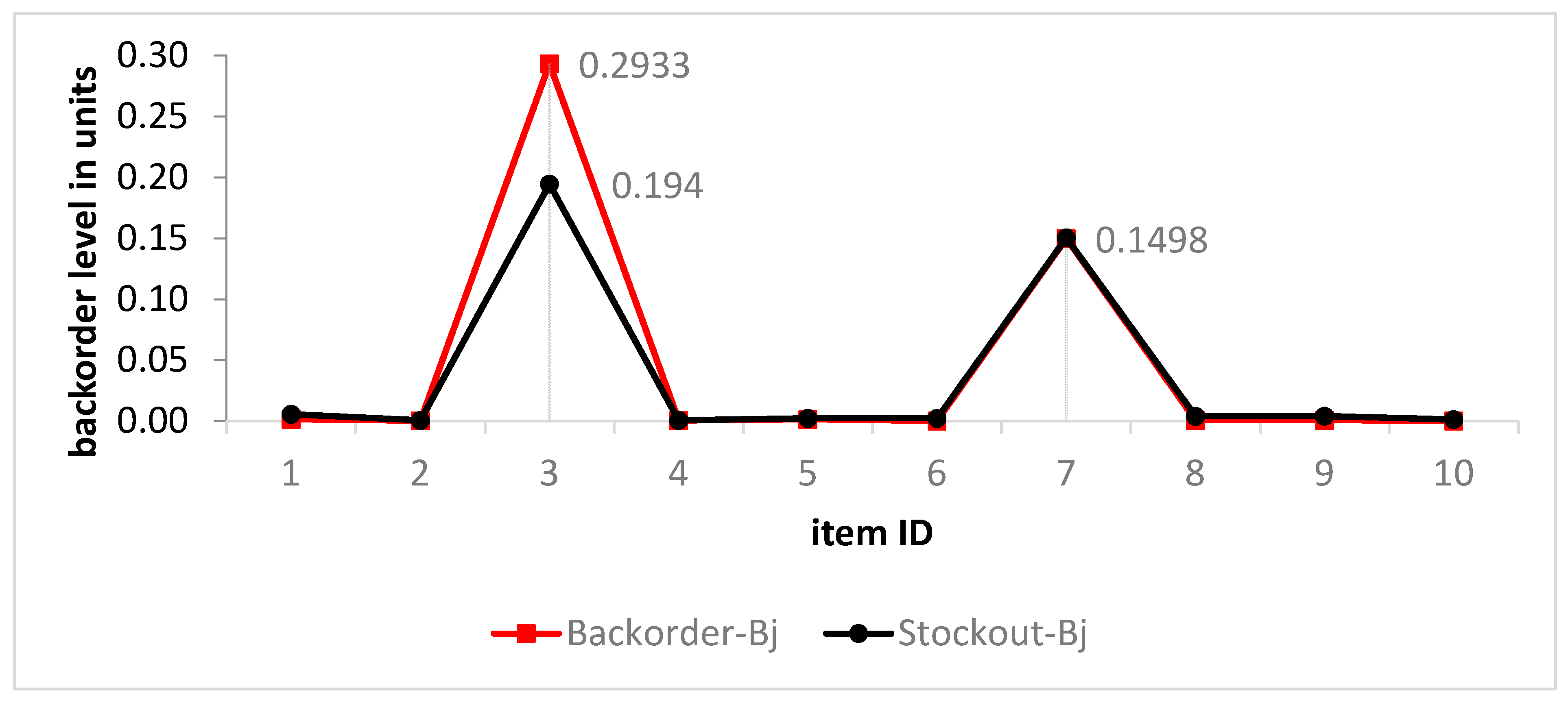
From Figure 4, it is clear that items 3 and 7 are critical in the ten items inventory and have low annual consumption history. The (Q, r) stock-out and backorder cost approach both focuses on the expensive inventory and low demand items to provide minimum inventory investment by assigning them low service level and high backorder level. The backorder cost model results in average inventory investment of USD 490,709 compared to the USD 491,535 value of the stock-out model. This is because of the different treatment of item number 3 in both models. For instance, the backorder model assigns the back order level of 0.2993 units to item 3 compared to the 0.194 units of backorder level in the stockout cost model. When the backorder level increases, the average inventory investment decreases.

The superiority of the stock-out model over the backorder model in achieving an average 98% service level with a minimum average inventory investment of USD 491,535 is because of assignment of low service level of 0.89% to item number 7 instead of assigning 91% service level as allocated by backorder model to item number 7 which results in high average inventory investment of USD 495,932. Both these models perform well in minimizing average inventory investment but selecting one of them depends on the company business nature. If the customer service is defined by the average fill rate, then the stock-out model is a better option and if the customer service is characterized by average backorder, then the best choice is the backorder model. This is because the stock-out cost model effectively utilizes the inventory to achieve the target fill rate (fraction of order filled from available stock) and the backorder cost model effectively uses the inventory in order to obtain the target level of the backorder.

4. Conclusions

In the multipart environment, defining the same service level for each item in the warehouse is not a good practice because some items have low consumption history and others have a high consumption rate. Therefore, the items that have low annual demand need a low service level in comparison with high annual demand. In this research, it is proven that the company’s existing Min–Max method assigns the same service level of 90% to each item in the inventory which results in high average inventory investment. Similarly, some items in the inventory are more expensive while others are less expensive, so the inventory of the expensive items requires tight control and continuous monitoring of the inventory level at the time of transaction from the available stock. Hence, in this research, the (Q, r) model is used based on continuous inventory review policy in both the stock-out cost approach and backorder cost approach to reduce the average inventory investment by assigning service level and backorder level to the items in the inventory based on their unit cost and yearly consumption history. In contrast, the company’s existing Min–Max method followed by a periodic inventory level review policy for the entire inventory is proved to be not a suitable approach for low demand and expensive items. This is because, in periodic review policy, the demand uncertainty is greater for which safety stock will be kept more than the continuous review policy in which less safety stock is kept due to less demand uncertainty [42]. Therefore, the average inventory investment of the company’s existing Min–Max method is greater than the proposed (Q, r) model.

It can be concluded that the (Q, r) model based on continuous inventory level review policy is the best choice for controlling inventory of the slow-moving and expensive inventory (Class A items) such as gate valve, and truck scale [25] instead of the company existing method and policy. The Min–Max method and the periodic inventory level review policy is best for inexpensive and fast-moving inventory (class B, C items) such as washers’ inventory, nut bolts, and other routine plant maintenance inventory. Based on the past seven-year actual consumption history (2009–2015) of the ten selected items of class A, the (Q, r) model stock-out cost approach results in an 8.88% increase in average service level and a 56.9% decrease in average investment. Similarly, the backorder cost approach of the (Q, r) model results in a 7.77% increase in the average service level and a 57% decrease in average inventory investment in comparison with the company existing inventory management model. Thus, the stock-out cost approach of the (Q, r) model is best for maintaining slow-moving and expensive inventory because of its high service level approximately at the same inventory investment to that of the backorder cost approach.

References

1. Li, L.; Liu, M.; Shen, W.; Cheng, G. An improved stochastic programming model for supply chain planning of MRO spare parts. Appl. Math. Model. 2017, 47, 189–207. [Google Scholar]
2. Uhlmann, E.; Bilz, M.; Baumgarten, J. MRO–challenge and chance for sustainable enterprises. Procedia CIRP 2013, 11, 239–244. [Google Scholar]
3. Takey, F.M.; Mesquita, M.A. Aggregate Planning for a Large Food Manufacturer with High Seasonal Demand. Braz. J. Oper. Prod. Manag. 2006, 3, 5–20. [Google Scholar]
4. Hassen, K.; Szucs, D. Supply Chain Optimization in the Oil Industry: A Case Study of MOL Hungarian Oil and Gas PLC. 2012. Available online: https://www.diva-portal.org/smash/record.jsf?pid=diva2%3A534394&dswid=-4076 (accessed on 24 September 2020).
5. Bevilacqua, M.; Ciarapica, F.E.; Giacchetta, G. Spare parts inventory control for the maintenance of productive plants. In Proceedings of the 2008 IEEE International Conference on Industrial Engineering and Engineering Management, Singapore, 8–11 December 2008; pp. 1380–1384. [Google Scholar]
6. Guajardo, M.; Rönnqvist, M.; Halvorsen, A.M.; Kallevik, S.I. Inventory management of spare parts in an energy company. J. Oper. Res. Soc. 2015, 66, 331–341. [Google Scholar]
7. Snyder, R.D.; Ord, J.K.; Beaumont, A. Forecasting the intermittent demand for slow-moving inventories: A modelling approach. Int. J. Forecast. 2012, 28, 485–496. [Google Scholar]
8. Dolgui, A.; Pashkevich, M. Demand forecasting for multiple slow-moving items with short requests history and unequal demand variance. Int. J. Prod. Econ. 2008, 112, 885–894. [Google Scholar]
9. Bacchetti, A.; Perona, M.; Saccani, N. Spare parts inventory and demand management. Comparing theoretical approaches with managerial practice. In Proceedings of the International Annual EurOMA Conference, Chalmers University of Technology, Göteborg, Sweden, 14–17 June 2009; pp. 1–10. [Google Scholar]
10. Turrini, L.; Meissner, J. Spare parts inventory management: New evidence from distribution fitting. Eur. J. Oper. Res. 2019, 273, 118–130. [Google Scholar]
11. Inderfurth, K.; van der Laan, E. Leadtime effects and policy improvement for stochastic inventory control with remanufacturing. Int. J. Prod. Econ. 2001, 71, 381–390. [Google Scholar]
12. Kabir, A.Z.; Al-Olayan, A.S. A stocking policy for spare part provisioning under age based preventive replacement. Eur. J. Oper. Res. 1996, 90, 171–181. [Google Scholar]
13. Kennedy, W.J.; Patterson, J.W.; Fredendall, L.D. An overview of recent literature on spare parts inventories. Int. J. Prod. Econ. 2002, 76, 201–215. [Google Scholar]
14. Persson, F.; Saccani, N. Managing the after-sales logistic network–a simulation study. Prod. Plan. Control 2009, 20, 125–134. [Google Scholar] [CrossRef]
15. Chima, C.M. Supply-chain management issues in the oil and gas industry. J. Bus. Econ. Res. (JBER) 2007, 5. [Google Scholar] [CrossRef]
16. Spearman, M.L.; Hopp, W.J. Factory Physics: Foundations of Manufacturing Management. Irwin Chic. IL 1996, 1, 230–231. [Google Scholar]
17. Kot, S.; Grondys, K.; Szopa, R. Theory of inventory management based on demand forecasting. Pol. J. Manag. Stud. 2011, 3, 148–156. [Google Scholar]
18. Tapia-Ubeda, F.J.; Miranda, P.A.; Roda, I.; Macchi, M.; Durán, O. Modelling and solving spare parts supply chain network design problems Modelling and solving spare parts supply chain network design problems. Int. J. Prod. Res. 2020, 7543, 1–21. [Google Scholar]
19. Irene, R.; Marco, M.; Orlando, D. An Inventory-Location Modeling Structure for Spare Parts Sites Supply Chain Network Design Problems in Industrial End-User Sites. IFAC Pap. 2018, 51, 968–973. [Google Scholar]
20. Cárdenas-barrón, L.E.; Shaikh, A.A.; Tiwari, S.; Treviño-garza, G. An EOQ inventory model with nonlinear stock dependent holding cost, nonlinear stock dependent demand and trade credit. Comput. Ind. Eng. 2020, 139, 105557. [Google Scholar] [CrossRef]
21. Rodrigues, L.R.; Yoneyama, T. A spare parts inventory control model based on Prognostics and Health monitoring data under a fill rate constraint. Comput. Ind. Eng. 2020, 148, 106724. [Google Scholar] [CrossRef]
22. Taylor, P.; Conceição, S.V.; Luis, G.; Lu, D.; Ramos, N.T.; Pedrosa, G.C. Production Planning & Control: The Management of Operations A demand classification scheme for spare part inventory model subject to stochastic demand and lead time. Proc. Plan. Control 2015, 37–41. [Google Scholar] [CrossRef]
23. Gu, J.; Zhang, G.; Li, K.W. Journal of Air Transport Management Ef fi cient aircraft spare parts inventory management under demand uncertainty. J. Air Transp. Manag. 2015, 42, 101–109. [Google Scholar] [CrossRef] [Green Version]
24. Papersonline, I.; Sérgio, P. Evolutionary Optimization of Spare Parts Inventory Policies: A Life Cycle Costing Perspective. IFAC Pap. 2019, 52, 2243–2248. [Google Scholar]
25. Duran, O.; Sérgio, P.; Pereira, L. An activity based costing decision model for life cycle economic assessment in spare parts logistic management. Int. J. Prod. Econ. 2019, 222, 107499. [Google Scholar] [CrossRef]
26. Keivanpour, S.; Kadi, D.A.; Vc, B.C. The Effect of “Internet of Things” on Aircraft Spare Parts Inventory Management Management. IFAC Pap. 2019, 52, 2343–2347. [Google Scholar] [CrossRef]
27. Sahin, M.; Eldemir, F. Application of Q-R Policy for Non-smooth Demand in the Aviation Industry. In Industrial Engineering in the Industry 4.0 Era. Lecture Notes in Management and Industrial Engineering; Calisir, F., Camgoz Akdag, H., Eds.; Springer: Cham, Switzerland, 2018. [Google Scholar] [CrossRef]
28. Stip, J.; Van Houtum, G.J. On a method to improve your service BOMs within spare parts management. Int. J. Prod. Econ. 2020, 221, 107466. [Google Scholar] [CrossRef]
29. Sheikh-Zadeh, A.; Farhangi, H.; Rossetti, M.D. Inventory grouping and sensitivity analysis in multi-echelon spare part provisioning systems. Comput. Ind. Eng. 2020, 143, 106230. [Google Scholar] [CrossRef]
30. Abuizam, R.; Thomopoulos, N.T. Adjusting an Existing Forecasting Model When Some Future Demands Are Known In Advance: A Bayesian Technique. J. Bus. Econ. Res. (JBER) 2006, 4. [Google Scholar] [CrossRef] [Green Version]
31. Sherbrooke, C.C. Metric: A Multi-Echelon Technique for Recoverable Item Control. Oper. Res. 1968, 16, 122–141. [Google Scholar] [CrossRef] [Green Version]
32. Patriarca, R.; Hu, T.; Costantino, F.; Di Gravio, G.; Tronci, M. A System-Approach for Recoverable Spare Parts Management Using the Discrete Weibull Distribution. Sustainability 2019, 11, 5180. [Google Scholar] [CrossRef] [Green Version]
33. Costantino, F.; Di Gravio, G.; Patriarca, R.; Petrella, L. Spare parts management for irregular demand items. Omega 2018, 81, 57–66. [Google Scholar] [CrossRef]
34. Nameirakpam, C.; Das Mohapatra, A.K. Effect of Career Stage on Organizational Commitment: Evidence from Selected Commercial Banks Operating in Manipur State of India. Saudi J. Bus. Manag. Stud. (SJBMS) 2018, 3, 186–191. [Google Scholar] [CrossRef]
35. Bacchetti, A.; Saccani, N. Spare parts classification and demand forecasting for stock control: Investigating the gap between research and practice. Omega 2012, 40, 722–737. [Google Scholar] [CrossRef]
36. Teixeiraa, C.; Lopesa, I.; Figueiredoa, M. Multi-criteria classification for spare parts management: A case study. Procedia Manuf. 2017, 11, 1560–1567. [Google Scholar] [CrossRef]
37. Hopp, W.J.; Spearman, M.L. Factory Physics, 2nd ed.; Waveland Press: Long Grove, IL, USA, 2000. [Google Scholar]
38. Heizer, J.; Render, B. Operations Management; Pearson Prentice-Hall: Upper Saddle River, NJ, USA, 2013. [Google Scholar]
39. Borade, A.B.; Ardak, P.S. A State of art on economic production quantity models. Braz. J. Oper. Prod. Manag. 2017, 14, 183–186. [Google Scholar] [CrossRef] [Green Version]
40. Zeng, S.; Nestorenko, O.; Nestorenko, T.; Morkūnas, M.; Volkov, A.; Baležentis, T.; Zhang, C. EOQ for perishable goods: Modification of Wilson’s model for food retailers. Technol. Econ. Dev. Econ. 2019, 25, 1413–1432. [Google Scholar] [CrossRef] [Green Version]
41. Gill, S.; Khullar, P.; Singh, N.P. A Review on Various Approaches of Spare Parts Inventory Management System. Indian J. Sci. Technol. 2016, 9, 1–5. [Google Scholar] [CrossRef]
42. Pinçe, Ç.; Dekker, R. An inventory model for slow moving items subject to obsolescence. Eur. J. Oper. Res. 2011, 213, 83–95. [Google Scholar] [CrossRef] [Green Version]
Figure 1. ABC Classification.
Sustainability 12 08027 g001
Figure 2. Sample of ten items Pareto Analysis.
Sustainability 12 08027 g002
Figure 3. Tradeoff curve (Backorder cost Model) for average ordering frequency of 2, 6, 9 and 12.
Sustainability 12 08027 g003
Figure 4. Item Unit Cost (Cj) vs. Annual Demand (Dj).
Sustainability 12 08027 g004
Figure 5. Order frequency (per year) vs. Service Level (1 means 100%).
Sustainability 12 08027 g005
Figure 6. Comparison of the model results.
Sustainability 12 08027 g006
Figure 7. Inventory investment with respect to service level and backorder level.
Sustainability 12 08027 g007
Figure 8. Graph based on achieving an average of 0.4 units Backorder Level.
Sustainability 12 08027 g008
Figure 9. Graph based on achieving an average service level of 98%.
Sustainability 12 08027 g009