Analysis of Variance Amplification and Service Level in a Supply Chain with Correlated Demand


1
Mechanical Engineering Department, Faculty of Engineering, Fayoum University, Fayoum 63514, Egypt
2
Department of Mechanical Design and Production, Faculty of Engineering, Cairo University, Giza 12613, Egypt
3
Mechanical and Aerospace Engineering Department, Sapienza University of Rome, Via Eudossiana, 18, 00184 Rome, Italy
*
Author to whom correspondence should be addressed.
Sustainability 2020, 12(16), 6470; https://doi.org/10.3390/su12166470
Submission received: 13 July 2020
/
Revised: 7 August 2020
/
Accepted: 7 August 2020
/
Published: 11 August 2020
(This article belongs to the Special Issue Inventory Management for Sustainable Industrial Operations)
Abstract
:The bullwhip effect reflects the variance amplification of demand as they are moving upstream in a supply chain, and leading to the distortion of demand information that hinders supply chain performance sustainability. Extensive research has been undertaken to model, measure, and analyze the bullwhip effect while assuming stationary independent and identically distributed (i.i.d) demand, employing the classical order-up-to (OUT) policy and allowing return orders. On the contrary, correlated demand where a period’s demand is related to previous periods’ demands is evident in several real-life situations, such as demand patterns that exhibit trends or seasonality. This paper assumes correlated demand and aims to investigate the order variance ratio (OVR), net stock amplification ratio (NSA), and average fill rate/service level (AFR). Moreover, the impact of correlated demand on the supply chain performance under various operational parameters, such as lead-time, forecasting parameter, and ordering policy parameters, is analyzed. A simulation modeling approach is adopted to analyze the response of a single-echelon supply chain model that restricts return orders and faces a first order autoregressive demand process AR(1). A generalized order-up-to policy that allows order smoothing through the proper tuning of its smoothing parameters is applied. The characterization results confirm that the correlated demand affects the three performance measures and interacts with the operating conditions. The results also indicate that the generalized OUT inventory policy should be adopted with the correlated demand, as its smoothing parameters can be adapted to utilize the demand characteristics such that OVR and NSA can be reduced without affecting the service level (AFR), implying sustainable supply chain operations. Furthermore, the results of a factorial design have confirmed that the ordering policy parameters and their interactions have the largest impact on the three performance measures. Based on the above characterization, the paper provides management with means to sustain good performance of a supply chain whenever a correlated demand pattern is realized through selecting the control parameters that decrease the bullwhip effect.
1. Introduction
Supply chains consist of multiple partners that collaborate to satisfy customer demand. The demand information flows in the upstream direction of supply chains in the form of replenishment orders so that each partner receives the orders from the immediate downstream partner(s) and places his orders with the adjacent upstream partner(s). Subsequently, the product flows through the downstream direction to satisfy the partner’s orders and eventually satisfying the customer demand. This is the common form of coordination in supply chains. The ideal situation is to achieve and sustain the best balance between the supply and demand throughout the supply chain at minimum cost. However, in most situations, the required balance is missing and hard to achieve due to the unpredictability of the supply chain response under various operational conditions [1,2].
Supply chains face a common problem, the so-called the demand information distortion, in which the demand variability is amplified as demand information moves upstream in supply chain. This problem is known as the bullwhip effect, and may also be called ‘order variance amplification,’ ‘demand amplification,’ or the ‘Forrester effect.’ Several studies have empirically confirmed the existence of the bullwhip effect and its negative impacts on supply chain performance and sustainability [3,4]. The bullwhip effect is recognized to cause misalignment between demand and supply, resulting in severe supply chain deficiencies such as excessive production orders, high logistics and inventory costs, and increased inability to meet delivery schedules. The bullwhip effect increases production costs since a highly oscillating order pattern, forces a production plan to change frequently, leading to a higher average production (capacity) costs per period [5]. These consequences of the bullwhip effect affect the balance of the supply chains and hinder their techno-economic sustainability [4,6]. Moreover, as industries are becoming more obliged to greenability [7], the link between bullwhip and the environmental consequences in terms of pollution and carbon emissions have been investigated [8]. Therefore, numerous studies have been conducted to measure and analyze the bullwhip effect (measured as ratio of order variance to demand variance), investigate its causes, and evaluate remedies and mitigation approaches. Different mitigation solutions for the bullwhip effect, such as information sharing mechanisms and order smoothing policies, have been proposed [8,9]. Many other researchers have investigated the effectiveness of the smoothing ordering policies such as smoothing order-up-to (OUT) policy to eliminate the bullwhip effect [10,11,12].
Most of the previous modeling studies have assumed that demand is an independent and identically distributed (i.i.d) stochastic process, and have provided useful insights regarding the causes of the bullwhip effect and the mitigative solutions for such demand conditions [13]. A correlated demand exists whenever a period’s demand is correlated to (or dependent on) the last period’s demands, and the ‘independence’ assumption becomes not valid. Few studies have investigated the bullwhip effect in supply chain models with correlated demand, even though such demand process exists in many real-life supply chains. Several researches have confirmed empirically the existence of correlated demand patterns [14,15,16,17,18,19]. Lee, So, and Tang [15] reported that the first order autoregressive (AR(1)) demand process was found to match the sales patterns of 150 SKUs (Stock Keeping Units) in a supermarket in UK. In particular, they have analyzed the weekly sales pattern of 165 SKUs over a two-year period. By conducting the Durbin-Watson test, they have found that the sales pattern of 150 SKUs (out of 165 SKUs) have autocorrelation with statistical significance. Moreover, they have found that all of the 150 SKUs have positive autocorrelation coefficients that vary between 0.26 and 0.89. Lee, Padmanabhan, and Whang [14] have also reported that it is common to have positive autocorrelation in the high-tech industry. Erkip, Hausman, and Nahmias [20] have also found that the demands of consumer products are often correlated over time with autocorrelation as high as 0.7. Therefore, most of the obtained results and characteristics of the bullwhip effect for independent demand need to be revised for correlated demand through conducting further research.
Research in correlated demand has attempted to model, measure, and analyze the bullwhip effect in supply chains that employ the classical OUT policy while using different forecasting methods [8,19,21,22,23]. Most of those studies have been relying upon statistical modeling approaches, and therefore they have been confined to the analysis of the bullwhip effect only and the so-called order variance ratio [18,19]. Moreover, for mathematical tractability, most of the previous studies for both correlated and uncorrelated demand have considered linear supply chains in which negative replenishment orders and open return policy are permitted [8,19,24,25,26,27,28]. Very limited research has been devoted to study the impact of correlated demand on both the bullwhip effect and inventory performance in supply chains that restrict negative replenishment orders. The inventory performance can be measured in terms of net stock amplification ratio (measured as ratio of net stock variance to demand variance), and service level (measured as average fill rate). The net stock variance ratio has an impact on inventory costs since increased inventory variance leads to a higher inventory cost to satisfy a desired service level. Analytical modeling studies have shown that when the demand is i.i.d, then using the smoothing OUT inventory policy will reduce the bullwhip effect. However, this may affect the inventory variance, and thus more inventory will be required to satisfy the desired service level [5,26]. Other studies have indicated that the order rate smoothing can be beneficial to both the bullwhip effect and inventory performance for the sustainability of supply chains of correlated demand [12,28].
The objectives of this paper are two-fold. First, the impact of correlated demand on supply chain performance in terms of order variance ratio, net stock variance ratio, and average fill rate is investigated. Second, the mutual impact of the key supply chain parameters and correlated demand is investigated. Examples of supply chain parameters are the lead-time, forecasting parameters, and ordering policy parameters. Most of the previous research assumes that a supply chain employs the classical OUT inventory policy with a specific forecasting method in response to AR(1). Alternatively, this research investigates the effect of the autoregressive demand under both the classical and generalized OUT ordering policies that are similar to those applied for i.i.d demand in previous studies [11,26]. The generalized policy is a modified version of the classical OUT policy that involves two smoothing parameters (also known as proportional controllers) to regulate the reaction to demand and inventory changes, and thus allowing order smoothing. The two smoothing parameters (Ti and Tw) can be controlled to alter the performance of the ordering policy. Furthermore, this paper investigates the impact of correlated demand not only on the bullwhip effect but also on the inventor stability and service level.
Due to the complexity and stochastic nature of supply chains under correlated demand, a simulation model approach is considered to study the impact of the correlated demand on the three mentioned performance measures. We mainly simulate the response of a single echelon supply chain that employs the generalized OUT policy, and use the exponential smoothing forecasting method to predict demand. A nonlinear supply chain that restricts return orders (negative orders) is assumed. The simulation model is utilized to characterize the supply chain performance in terms of order variance ratio (OVR), net stock amplification ratio (NSA), and average fill rate/service level (AFR), under various operating conditions. Furthermore, a full factorial experiment is conducted to investigate the mutual impact of the other supply chain parameters and their interactions with demand correlation. The characterization results confirm that the correlated demand affects the three performance measures and interacts with the key supply chain parameters. The OVR and NSA results under the classical OUT policy are consistent with the published results in the literature, except when the demand is negatively correlated due to the assumption of return order restriction [23]. Most importantly, the characterization results indicate that the generalized OUT policy should be adopted with the correlated demand, as its smoothing parameters can be tuned to utilize the demand characteristics such that OVR and NSA can be reduced without affecting the service level (AFR). The characterization results are complemented with a full factorial experiment that focused only on the positively correlated demand and the other operational parameters (lead-time, forecasting parameter, and ordering policy parameters). The related ANOVA results indicate that all the investigated factors and their interactions have significant impacts on OVR and NSA. In particular, the ordering policy parameters are found to have the largest impact on OVR, NSA, and AFR. The ANOVA results also confirm that the unmatched smoothing parameters of the OUT inventory control policy will provide better OVR and NSA than the matched case for the positively correlated demand.
This paper contributes to the existing supply chain literature through providing a comprehensive analysis of supply chain performance in the presence of AR(1) demand process. The paper has investigated the impact of the generalized OUT policy on OVR, NSA, and AFR such that the trade-off between bullwhip effect and inventory performance can be analyzed under demand correlation. Previous research has always assumed the presence of independent demand and has indicated that the mitigation of OVR will be coupled with an increase in NSA, and thus a lower AFR will be gained unless safety stock is increased. This paper has provided the evidence that under certain correlated demands, such as AR(1), the mitigation of both OVR and NSA can be achieved. As such, it is expected that the findings of this research shall help management to apply the recommended ordering policies and forecasting methods whenever demand is correlated, and avoid using the classical recommendations for independent demand situations. The application of the proper policies and forecasting methods to control a supply chain should sustain its performance measures at their planned levels.
The paper is structured as follows: Section 2 presents the related literature review. Section 3 describes the supply chain model and the corresponding simulation model. The performance characterization results are presented and discussed in Section 4. The experimental design and the related ANOVA results are presented and analyzed in Section 5. The conclusions and future research direction are provided in Section 6.
2. Literature Review
Several studies have empirically confirmed the existence of the variance amplification of demand in real-life supply chains [3,5,11,14,29,30,31]. In addition, other studies have resorted to simulation games to prove the existence and to analyze the bullwhip effect [32,33,34,35,36]. Other research is directed to identify and analyze its causes. Research in operational causes of the bullwhip effect includes demand signal processing, batched orders, lead-time, price fluctuations, and rationing and shortage gaming [35].
Extensive modeling research has been conducted to measure and analyze the variance amplification utilizing several modeling methodologies such as analytical modeling [19,22,38,39], control theory modeling [10,11,28,40], and simulation modeling [24,41,42]. Most research in this direction assumes that demand is an independent and identically distributed (i.i.d) stochastic process. Dejonckheere et al. [11] confirmed through a control theoretic modeling approach that the classical OUT inventory policy with exponential smoothing (ES), moving average (MA), or demand signal processing forecasting will produce bullwhip for all demand patterns. However, they also showed that the classical OUT policy can be modified into a smoothing OUT policy, i.e., one that is able to produce replenishment orders with less variance than the demand. Chatfield et al. [40] used simulation to analyze the impact of the stochastic lead time, the information sharing, and the quality of the information on the bullwhip effect, assuming i.i.d normal demand process. Canella [42] used simulation to investigate and compare the behavior of classical and smoothing OUT ordering policies in an information exchange supply chain with i.i.d normal demand process. Several other studies have investigated the effect of forecasting [43], ordering policy [44], lead-time [24], and collaboration [41,44,45], while assuming i.i.d demand process. Those studies have provided useful insights regarding the bullwhip effect causes and mitigation solutions under such demand conditions.
Although the assumption of i.i.d demand has some mathematical advantages, it neglects correlation in a demand time series. Therefore, another research stream has considered correlated demand models such as autoregressive integrated moving average (ARIMA) and its variants [8]. In particular, the first order auto-regressive demand, AR(1), has been the most frequently adopted demand model in the relevant literature [8,19]. In addition, most of these studies have assumed that the supply chain employs the classical OUT policy with the minimum mean squared error (MMSE) forecasting method, and permits the return orders (negative orders) [46,47,48]. Luong [21] derived a bullwhip effect measure for a single-echelon supply chain that has AR(1) demand process and employs the classical OUT policy with the MMSE forecasting method. Similarly, Luong and Phien [47] quantified the bullwhip effect for AR(2) demand process and extended their results to autoregressive demand processes of higher orders (AR(q)). Sirikasemsuk and Luong [48] derived a bullwhip effect measure for a first-order bivariate vector autoregression (VAR(1)) demand process in a two-stage supply chain. Those studies have provided useful results concerning the behavior of the bullwhip effect with respect to autoregressive coefficients and lead-time when the supply chain employs the classical OUT policy with MMSE forecasting method and permits the negative orders. In particular, for the AR(1) demand process, they have shown that the bullwhip effect will not exist for the uncorrelated demand (i.i.d. demand, , where is the autocorrelation coefficient of demand), negatively correlated demand (), or perfect positively correlated demand (). They have also shown that the bullwhip effect increases as lead-time increases and there is an upper bound for the bullwhip effect increase that depends on the autocorrelation level. However, these studies have focused only on the bullwhip effect measure and therefore they have been relying on analytical modeling approaches. Further similar studies can be found in Chandra and Grabis [49], and Duc, Luong, and Kim [22].
Unlike the above researches, other correlated demand studies have investigated analytically the performance of the classical OUT policy when integrated with other common forecasting methods such as moving average (MA) and exponential smoothing (ES) [18,28]. Chen, Ryan, and Simchi-Levi [37] and Chen et al. [50] derived analytically the bullwhip effect expressions for both the MA and ES forecasting methods in a supply chain employing the classical OUT policy and facing AR(1). They have also compared the impact of the two forecasting methods on the bullwhip effect. Zhang [46] derived analytical expressions for the bullwhip effect under AR(1) with MA, ES, and MMSE forecasting methods. Ma et al. [51] derived analytically the measures of bullwhip effect and inventory variance for MMSE, MA, and ES under price sensitive AR(1) demand. As stated earlier, these researches have adopted an analytical modeling approach and therefore most of them have focused only on modeling and analyzing the bullwhip effect. They have confirmed that the selected forecasting method has a significant role in determining the effect of lead-time and demand autocorrelation on the bullwhip effect. In particular, they have shown that the impact of reducing lead-time on the bullwhip effect depends on the correlation level and forecasting method, and therefore decision makers should be aware of the underlying demand process and the forecasting method used before making such decisions regarding lead-time reduction.
Other researchers have resorted to simulation modeling to study the impact correlated demand on different measures of supply chain performance. Hussain, Shome, and Lee [23] conducted a simulation study to investigate and compare the impact of ES and MMSE on both the bullwhip effect and inventory variance in a single-echelon supply chain that faces AR(1) demand process, employs the classical OUT policy, and permits return orders. They have concluded that depending on the demand correlation, the appropriate selection of forecasting method can help in controlling the bullwhip effect. However, they have also shown that the inventory variances with ES are greater than inventory variances with MMSE and that the gap increases as lead-time increases. Campuzano-Bolarín et al. [52] also performed a simulation study to compare the impact of six different forecasting methods on the bullwhip effect, net stock amplification, and fill rate. Costantino et al. [53] developed a control chart-based forecasting mechanism and compared its performance with MA and ES in a multi-echelon supply chain that employs the classical OUT policy and faces AR(1) demand process, through a simulation study.
Some other researchers attempted to study the bullwhip effect under correlated demand with different inventory ordering policies other than the classical OUT policy. Bandyopadhyay and Bhattacharya [54] derived analytically bullwhip effect measures for ARMA(p,q) demand process under various inventory replenishment policies. Disney et al. [28] have quantified exactly the bullwhip effect, and the variance of inventory levels over time, for i.i.d. and the weakly stationary autoregressive (AR), moving average (MA), and autoregressive moving average (ARMA) demand processes under the generalized OUT policy. Gaalman and Disney [55] analyzed the behavior of the proportional order-up-to policy for ARMA(2,2) demand with arbitrary lead-times.
The literature review shows that most of the correlated demand research has focused mainly on the modeling, measuring, and analysis of the bullwhip effect in linear supply chains. Most of the previous studies have adopted analytical modeling approach, and therefore their scope has been limited to the analysis of the bullwhip effect for supply chains that allow return orders. Few studies have been directed to the modeling and analysis of both the bullwhip effect and the inventory performance measures (net stock amplification and service level). Moreover, most of the previous research has been devoted to investigating the impact of correlated demand in supply chains that employ the classical OUT policy with different forecasting methods. Limited studies have attempted to investigate the impact of other ordering policies, such as the generalized OUT policy, which is a highly recommended ordering policy to mitigate the bullwhip effect for i.i.d demand. The literature is lacking studies that have attempted to investigate the impact of correlated demand and the mutual impacts of other operational parameters with correlated demand.
3. Model Development
In this section, the single-echelon supply chain model, including ordering policy, forecasting method, demand model, and performance measures, is described. In addition, the simulation model of the considered supply chain model is presented to validate the results.
3.1. Supply Chain Model
A generic single-echelon supply chain that may represent a retailer, distributor, or manufacturer is modeled. This supply chain structure has been widely adopted in related research [23,28]. It is assumed that this supply chain faces a first order autoregressive demand, AR(1), and employs the generalized order-up-to (OUT) policy with the exponential smoothing (ES) forecasting method. The supply chain operations are performed according to the following sequence of events and assumptions that are adapted from the literature. At each time period, the supply chain echelon (e.g., retailer) receives the products/materials from an upstream echelon (e.g., manufacturer), updates the available on-hand inventory, and satisfies the backlogged orders. Afterwards, the downstream echelon observes and updates the on-hand inventory level, and finally places a non-negative replenishment order, if needed. The replenishment order is determined based on the generalized order-up-to (OUT) policy. It is assumed that order returns (negative replenishment orders) are not allowed, and that the upstream echelon can deliver and ship any quantity ordered. Delivery lead-time is assumed deterministic.
3.1.1. Autoregressive Demand
We assume that the supply chain receives a first order autoregressive demand, AR(1), that can be defined as follows:
where is the AR(1) demand at time , stands for the mean of the AR(1) demand process, represents the error term which follows a normal distribution with and , and is an autoregressive (autocorrelation) coefficient, where . The variance of AR(1) demand can be approximated as , and when the demand process is independently and identically distributed (i.i.d), i.e., [46].
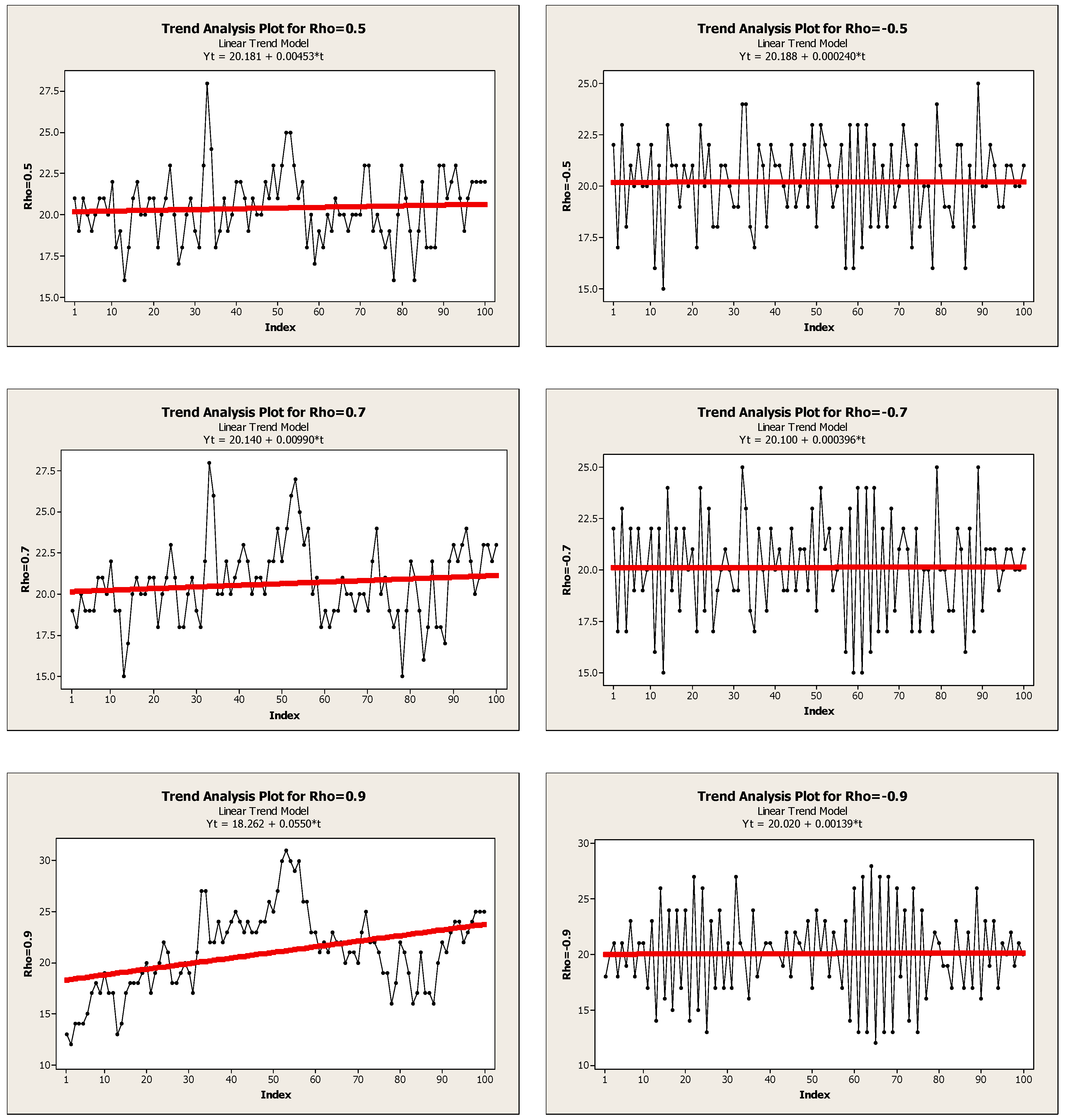
A demand generator module has been implemented in SIMUL8 to generate AR(1) demand patterns according to Equation (1). In particular, the generator can simulate the AR(1) demand process for any given combination of values of , , and . After validating the demand generator, several AR(1) demand times series have been simulated at different values of in order to reflect the specific characteristics of each demand process (see Figure 1). It can be observed that for the negatively correlated demand (), the demand time series exhibits period-to-period oscillatory behavior. In addition, the negatively correlated demand patterns are almost free of runs and do not develop any trends over time (see Figure 1). On the contrary, the positively correlated demand develops runs and shows trends that materialize as increases (see Figure 1).
3.1.2. The Generalized OUT Policy
The generalized order-up-to policy is a modified classical order-up-to (OUT) policy. The later policy is common in the literature of supply chain due to its industrial popularity [56]. In the classical OUT policy, the ordering decision is made at the end of each review period (R) as follows [11]:
where is a non-negative replenishment order placed at the end of period t, is the order-up-to level considered in period t, and is the inventory position which is equal to the net stock () plus on-order inventory or work in process (). The net stock represents the on-hand inventory minus backlogged orders. The order-up-to level is updated every period according to
where is the estimate of mean demand over the risk period ( where is an estimate of demand in the next period, and L is the risk period), and represents the safety stock component which accounts for demand variation over L. The risk period L encompasses the lead-time (Ld) and the review period (R). In this model, the safety stock is included by extending the risk period by a safety stock parameter k [11,28,57]. Accordingly, the order-up-to level is dynamically updated in every review period based on the demand forecast , and it can be expressed as shown in Equation (4).
The classical OUT policy’s ordering rule can be decomposed into several components as shown in Equation (5). In particular, the order decision based on the classical OUT policy consists of three components: a demand forecast term (assuming R = 1), a net stock discrepancy term, and a work in process (on-order inventory) discrepancy term. Thus, both discrepancy terms are completely taken into consideration in replenishment orders (see Equation (5)). However, previous studies have shown that the classical OUT policy with demand forecast updating would always result in a bullwhip effect for any demand process [10,11].
A proposed approach to enable order smoothing is to recover only fractions of the two discrepancy terms in each time period through adding the two proportional controllers and . This transforms the classical OUT policy into a generalized OUT policy that is defined as follows:
where denotes the target net stock level, and denotes the desired work in process at time t. Ti and Tw are two proportional controllers (also known as smoothing parameters).
The parameters Ti and Tw control how much of the discrepancy between actual inventory and target inventory, and how much of the discrepancy between actual work in process and target work in process should be incorporated in the replenishment order [5]. This ordering rule has been adopted as a mitigation solution for the bullwhip effect by tuning the values of Ti and Tw [11]. Most of the previous research has investigated this ordering policy with matched controllers (Ti = Tw) under i.i.d. demand process [12,28,42]. In this study, we allow using unmatched controller and investigate their interaction effect on supply chain performance.
3.1.3. Exponential Smoothing Forecast
The generalized OUT replenishment policy requires an estimate or a forecast of demand over the risk period () at the end of each time period. The demand forecast is computed by multiplying the estimate of the next period’s demand () by the risk period L. Exponential smoothing (ES) forecasting method is applied to estimate the expected demand (). ES has been the most employed forecasting method in the related research [28]. The ES method determines the next period’s demand forecast by adjusting this period’s forecast error with an exponential smoothing parameter as follows:
where is the forecast of next period’s demand made in period t, is the received demand at time t, and represents the exponential smoothing parameter (). It is known that a larger implies a greater weight is assigned to the most recent demand observation, while a smaller implies a greater weight is placed on the demand history in the forecast of next period’s demand.
3.1.4. Performance Measures
We consider three performance measures to assess the impact of correlated demand and of the other operational parameters on supply chain performance. The following performance measures are considered: order variance ratio (OVR), net stock amplification ratio (NSA), and average fill rate (AFR). Most of the previous research has considered only the impact of correlated demand on the OVR measure, and a limited research has been devoted to the analysis of NSA and AFR measures [19,23,41]. Thus, analyzing the three performance measures provides a wider perspective about the supply chain performance and its sustainability.
The order variance ratio (OVR) is defined as the ratio of the order rate variance to the demand variance [5]. It can be expressed mathematically as in Equation (8).
The net stock amplification ratio (NSA) refers to the ratio of the net stock variance to the demand variance as in Equation (9) [5,28].
The service level can be assessed through the measure of average fill rate (AFR) which estimates the proportion of the demand that can immediately be supplied from the on-hand inventory [12,42,57,58]. The proportion of the supplied demand (fill rate) in each time period () is calculated as shown in Equation (10), where represents the released shipment at time , expresses the initial backlog at time t, and is the received demand at time t, and t = 1, …, T.
The fill rate time series can be used to estimate the average fill rate (AFR), as expressed in Equation (11):
3.2. Simulation Model Validation
A simulation model for the above-described supply chain model has been implemented in SIMUL8. The complete simulation model includes demand generation module, forecasting module, ordering policy module, and performance measures estimation module. Several verification tests have been performed to ensure that these modules are working properly. Output validation tests have been conducted to ensure the validity and suitability of the simulation model for further analysis. In particular, the simulation model output is compared with the output of the closed form expressions derived by Chen, Ryan, and Simchi-Levi [37], and Disney et al. [28] (see Table 1). Chen, Ryan, and Simchi-Levi [37] derived analytically the OVR measure for a single-echelon supply chain that employs the classical OUT policy with the ES forecasting method, in response to AR(1) demand process. Disney et al. [28] quantified both the OVR and NSA measures for a similar supply chain model that employs the generalized OUT policy with matched smoothing parameters (Ti = Tw = Tn, where Tn is a single smoothing parameter to replace both Ti and Tw in Equation (6) for the matched controller case) under different forecasting methods. We consider their closed form expression for OVR and NSA under the mean demand forecasting method.
The validation tests are conducted at different values of that varies in the range of −0.9 and 0.9, while all the other model parameters are kept fixed. It is assumed that negative customer demand is not allowed, i.e., . Therefore, when simulating AR(1) demand, the mean demand is set much higher than to avoid negative demand realizations (e.g., ). In all the validation experiments, the demand pattern is generated with the following parameter settings: and . For the validation of OVR with Chen, Ryan, and Simchi-Levi [37] and Disney et al. [28], the simulation experiments are conducted at Ld = 2, k = 1, α = 0.1, and Tn = 1 (Ti = Tw = 1). The ES parameter is set to α = 0 for the validation with Disney et al. [28] since the demand forecast should be based on the long-term average demand ( This setting of the ES parameter transforms the ES method’s forecast to be the mean demand value. The simulation results are obtained by running the simulation model for five replications, with a replication length of 100,000 periods and a warm-up of 5000 periods. These simulation settings are chosen so that the precision level of the estimated performance measures is less than ±5% [26].
The validation results are summarized in Table 2 and Table 3. The simulation results indicate that the behavior of OVR for the positively correlated demand is very consistent with the analytical results. However, the OVR behavior for the negatively correlated demand is less consistent with the analytical results, especially at high correlation values. For the NSA measure, the simulation results are very consistent with those of the analytical results. As such, the existing analytical models for OVR that are based on the assumption of the presence of negative replenishment orders will overestimate the OVR under the negatively correlated demand especially at high correlation values. This result has also been confirmed for the i.i.d demand in multi-echelon supply chains [24,25]. Accordingly, simulation modeling provides an accurate estimation for the performance measures where supply chain nonlinearity can be easily and accurately considered in the simulation model.
4. Performance Characterization under Correlated Demand
Sets of simulation experiments are conducted to investigate the impact of the autoregressive parameter on the three measures of performance (OVR, NSA, and AFR), under various operating conditions. The first set of experiments is conducted to investigate the impact of (the demand correlation coefficient) on the performance measures under the classical OUT policy while considering different combinations of and Ld. The second set of experiments is devoted to analyzing the impact of under different settings of the ordering policy parameters (Ti and Tw), to allow the comparison between the classical and the smoothing OUT policies. For each simulation experiment, the simulation model is run for five replications with a replication length of 100,000 periods and a warm-up of 5000 periods. The other model parameters are set to and , and k = 1. The case of i.i.d. demand is included in each experiment by setting .
4.1. Analysis of the OVR Measure
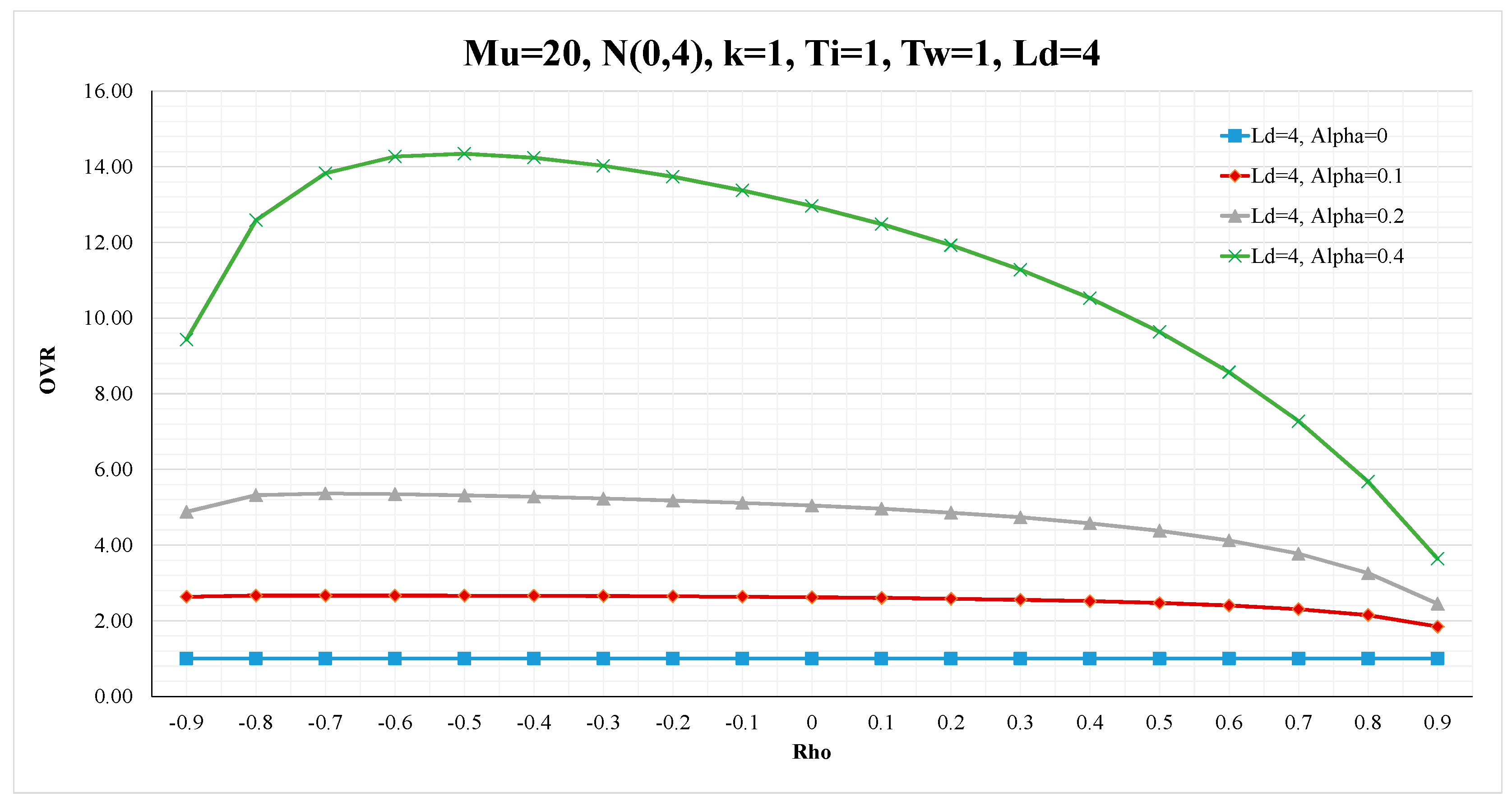
The simulation results of the OVR measure under the classical OUT policy for Ld = 2 and Ld = 4 are depicted in Figure 2. Results confirm that the bullwhip effect will not exist (i.e., OVR = 1), as long as there is no updating of demand forecast () regardless of the value of or Ld [11,28,37]. The setting of for the exponential smoothing forecast makes the demand forecast constant, and equals to the long-term average demand (), for all time periods. On the other hand, the bullwhip effect appears (OVR > 1) when demand forecast is updated () and it increases as increases, for all values of . Moreover, the results show that the negatively correlated demand produces a higher bullwhip effect than both the i.i.d demand and the positively correlated demand. The same behavior of OVR for the classical OUT with ES has been reported in Hussain, Shome, and Lee [23], and they have shown that the MMSE forecasting method will result in an increasing pattern of OVR over .
Furthermore, when the demand is positively correlated ( > 0), the OVR decreases as increases (see Figure 2). Especially for the highly positively correlated demand and when is large, the forecast shall follow the most recent highly correlated demand, and hence a smaller OVR value is realized as increases. On the contrary, for small , the demand process is stationary and reverses sign around its mean more frequently, and thus a large will produce higher deviations of the forecasts from the actual demand. For small ( = 0, = 0.1), OVR is not affected by (). However, when the demand is negatively correlated, the OVR increases as increases until it reaches to a maximum level and then decreases. For the highly negative correlation demand ( to ), the demand variance () becomes larger, but the order variance increases at a lesser rate, and thus making OVR smaller (see Equation (8)). Moreover, at highly negatively correlated demand, the likelihood of placing negative orders is high, and since it is assumed that all orders should be greater than or equal to zero (no return policy), the order variance is reduced, leading to the shown decline in OVR (see Table 4). The existing analytical models have shown that OVR will be an increasing function of over the negative correlation domain [24,28,37]. Accordingly, these analytical models are not recommended for estimating the OVR measure at highly negatively correlated demand as it will overestimate the actual bullwhip effect for this demand pattern.
Figure 2 also shows that the lead-time Ld contributes considerably to the OVR measure (bullwhip) regardless of the autocorrelation level. Moreover, the OVR measure is more sensitive to Ld and under the negatively correlated demand than under the positively correlated demand. For a given value of , doubling the lead-time (Ld = 4) increases the bullwhip effect almost proportionally. The long lead-time seems to amplify the reaction to demand changes, and thus the forecasting error of the lead-time demand will increase. In addition, as the lead-time increases, the actual demand () will be lagging the actual order size placed based on , thus, increasing the order variance and increasing the OVR (see Table 4). This is also evident from the closed form expressions for OVR in Table 1 where the effect of lead-time is related to the update of demand forecast.
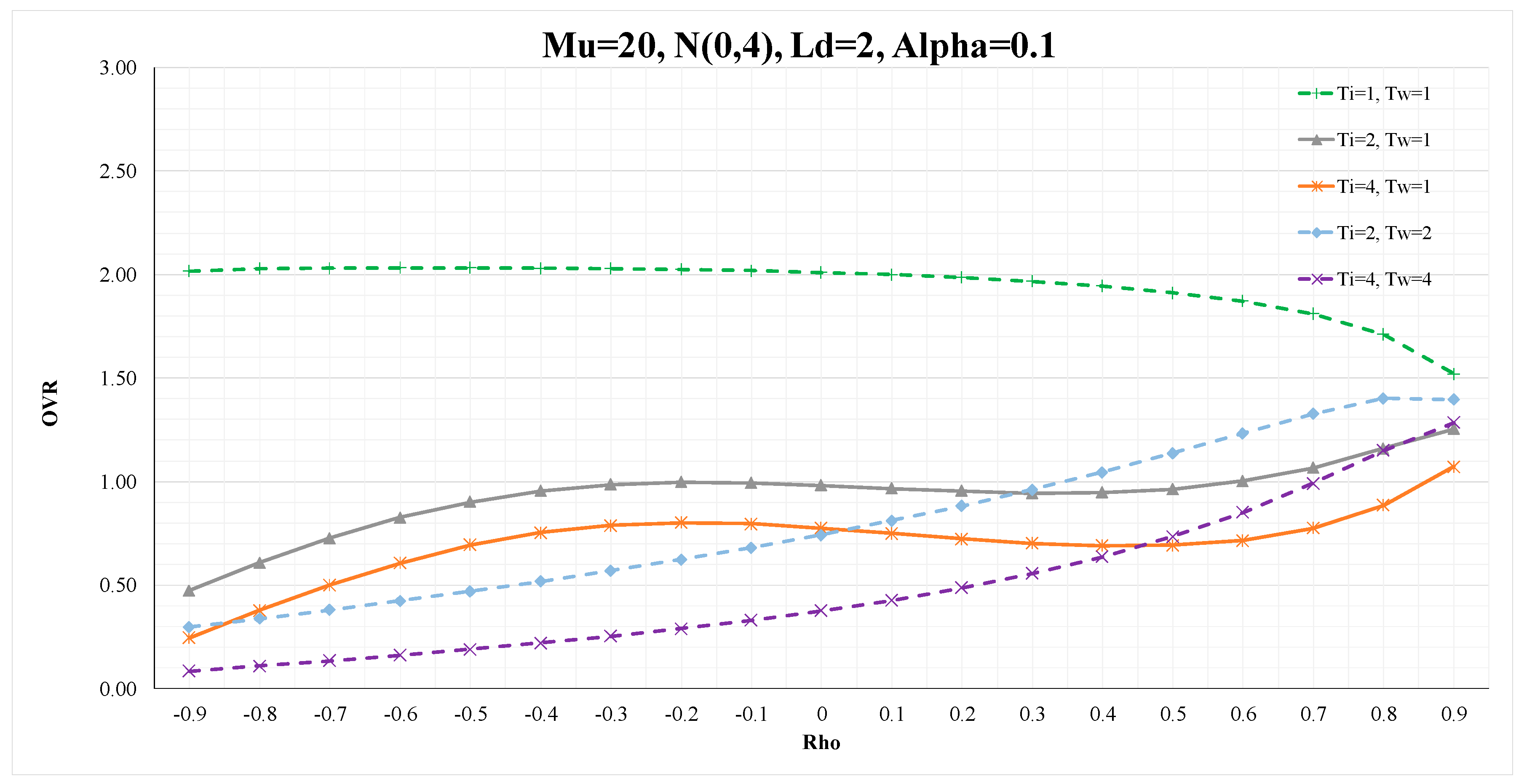
The impact of the parameters of the inventory ordering policy on OVR is shown in Figure 3. The effect of the ordering policy parameters (Ti and Tw) varies with the value of . In particular, the results confirm that the generalized OUT policy can mitigate and almost eliminate the bullwhip effect by the proper selection of the values of Ti and Tw. In this case, the generalized OUT policy is transformed into a smoothing OUT policy. For the negatively correlated and i.i.d demands, the best bullwhip effect is achieved when Ti = Tw > 1 and that increasing the levels of Ti and Tw leads to a lower OVR. This conclusion is also valid for demands with weak positive correlation. The equality of the two smoothing parameters is called a matched controller, and it has been the most investigated and recommended in the related studies that considered i.i.d. demand process [28]. However, for the highly positively correlated demand, the matched controller (Ti = Tw) is not the preferred setting for lowering the bullwhip effect. It can be seen that the settings “Ti > Tw” provide a lower OVR than “Ti = Tw.” These results extend the previous findings of Disney et al. [28] that considered the matched case. However, the results should be extended to investigate the interaction of the ordering policy parameters (Ti and Tw) and their interactions with the other operational parameters (including ). This will be accomplished though the factorial design study in Section 5.
The results of the OVR measure provide useful insights for the practitioners and decision makers. The practitioners should be aware of the demand pattern (correlated or uncorrelated), and if the demand is correlated, they should identify whether it’s positively or negatively correlated. A careful attention should be given to the negatively correlated demand, especially in supply chains that employ the classical OUT policy, since it leads to a higher OVR than the positively correlated demand. In addition, the negatively correlated demand shows a higher sensitivity to lead-time such that reducing the lead-time to improve the OVR measure is highly recommended for the negatively correlated demand. In other words, the benefits gained from reducing the lead-time depend on the demand correlation.
For a practitioner, he is advised to conduct further evaluation before investing in lead-time reduction, especially when the demand is positively correlated. Most importantly, a practitioner is advised to adopt the generalized OUT policy since it can mitigate/eliminate the bullwhip effect. In particular, a practitioner can easily adapt the classical OUT policy (which is commonly applied in real-life supply chains) into a generalized OUT policy by incorporating the two smoothing parameters Ti and Tw. They are also suggested to adapt the matched smoothing parameters for the negatively correlated demand, i.i.d demand and weak positively correlated demand. However, for the highly positively correlated demand, the unmatched smoothing parameters (Ti > Tw) may provide better results than the matched settings (Ti = Tw).
4.2. Analysis of the NSA Measure
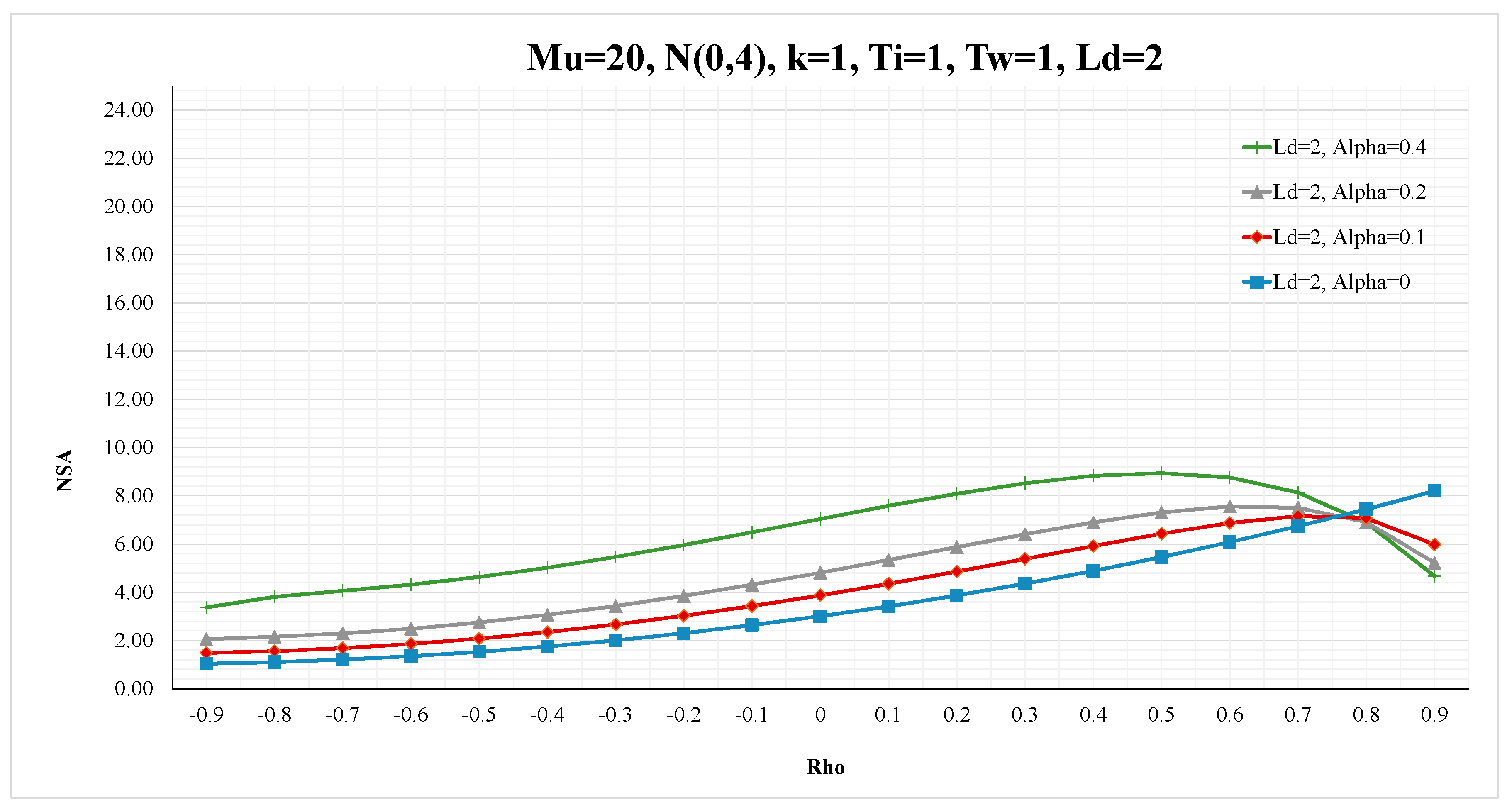
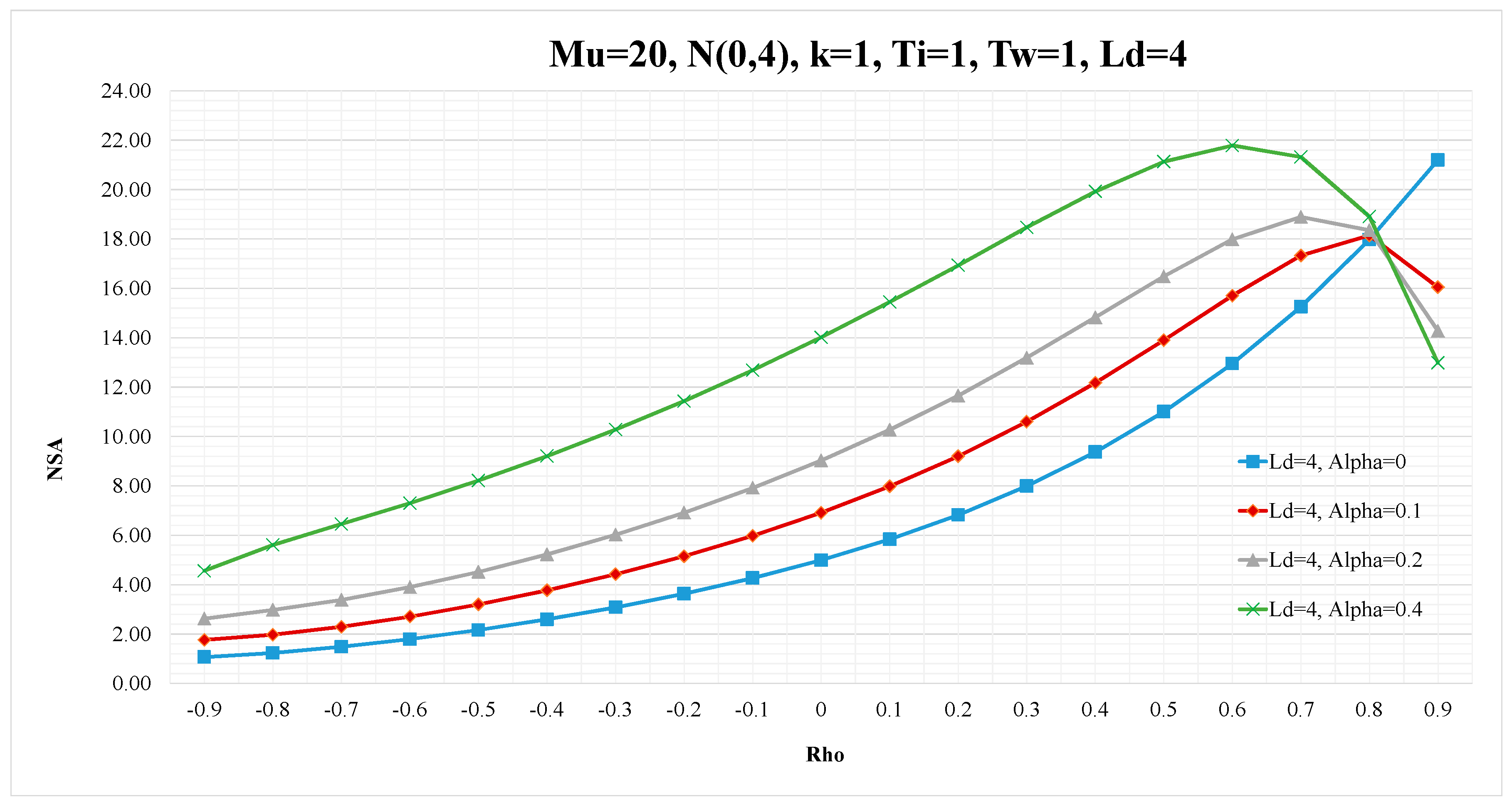
The impact of on NSA under the classical OUT policy is depicted in Figure 4. The results show that the positive correlation demand () produces a higher NSA than either the i.i.d. demand or the negatively correlated demand. Moreover, the i.i.d. demand has a higher NSA than the negative correlation demand. For , the NSA increases as increases until it reaches to a maximum level and then decreases. However, the NSA becomes an increasing function of when the demand forecast is based on the long-term average demand (). For , the NSA decreases as increases. The same behavior of NSA, with respect to the impact of under the classical OUT, is reported in Hussain, Shome and Lee [23] for both the ES and MMSE forecasting methods. Results indicate that the impact of ES forecasting becomes of significant value when the demand process is highly positively correlated (). The NSA increases with Ld and consistently but may decline after some cut-off value depending of the value of . Most likely, this can be explained by the developed trends at highly positively correlated demand (see Figure 1). As such, the over-reaction to demand changes will reduce the gap between the supply and demand and thus the net stock amplification ratio is reduced [28].
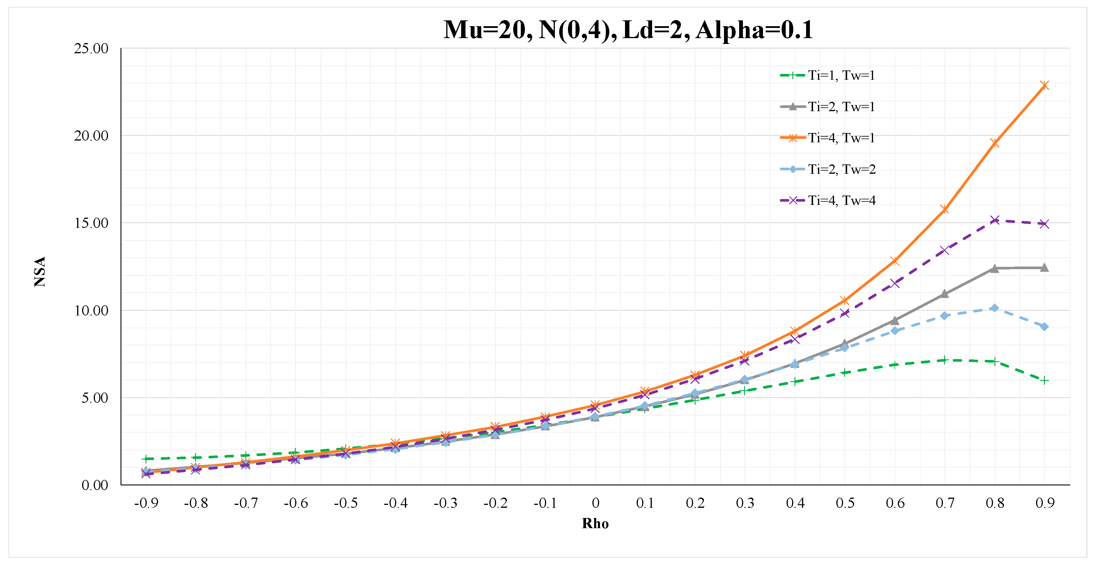
The impact of the ordering policy parameters on NSA is shown in Figure 5. The results indicate that the impact of the ordering policy parameters (Ti and Tw) depends on the value of . For the negatively correlated demand, the generalized OUT policy (with the smoothing settings of Ti and Tw) will lead to a lower NSA than the classical OUT policy (Ti = Tw = 1). In general, the effect of the different settings of the ordering policy parameters is within a narrow band for demand with . For such correlated demand, the results suggest that it is possible to utilize the flexibility of the generalized OUT policy to design inventory ordering policies that can lessen or avoid the bullwhip effect while achieving a comparable NSA. In particular, for the i.i.d and positively correlated demands, the results confirm that the smoothing OUT will result in a higher NSA than the classical OUT policy.
The results provide useful insights for the supply chain managers regarding the behavior of the inventory under correlated demand. It is known that the increase in NSA implies that the safety stock level should be increased to realize a desired service level (AFR). Therefore, the inventory costs will increase as NSA increases. For the NSA measure, the practitioners are advised to pay more attention to the positively correlated demand as it results in a higher NSA than the negatively correlated demand. They are suggested to use the classical OUT policy with the positively correlated demand while the smoothing OUT policy (with matched smoothing parameters) is highly recommended with the negatively correlated demand. The classical OUT policy will provide a good inventory performance with the positively correlated demand but it has undesirable performance with respect to the order variance ratio as discussed above. On the other side, the smoothing OUT policy will provide a good performance in terms of both OVR and NSA with the negatively correlated demand.
4.3. Analysis of the AFR Measure
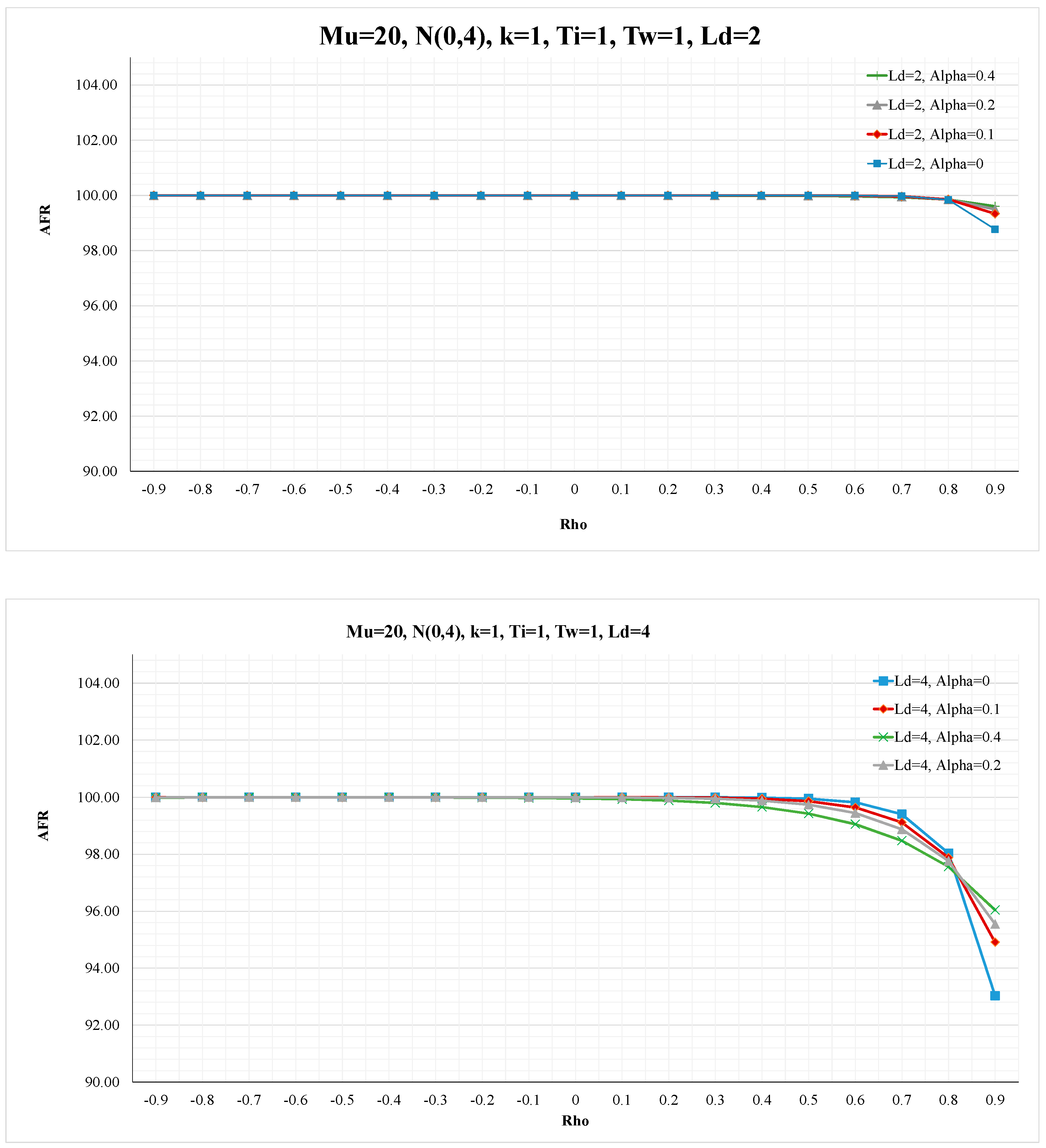
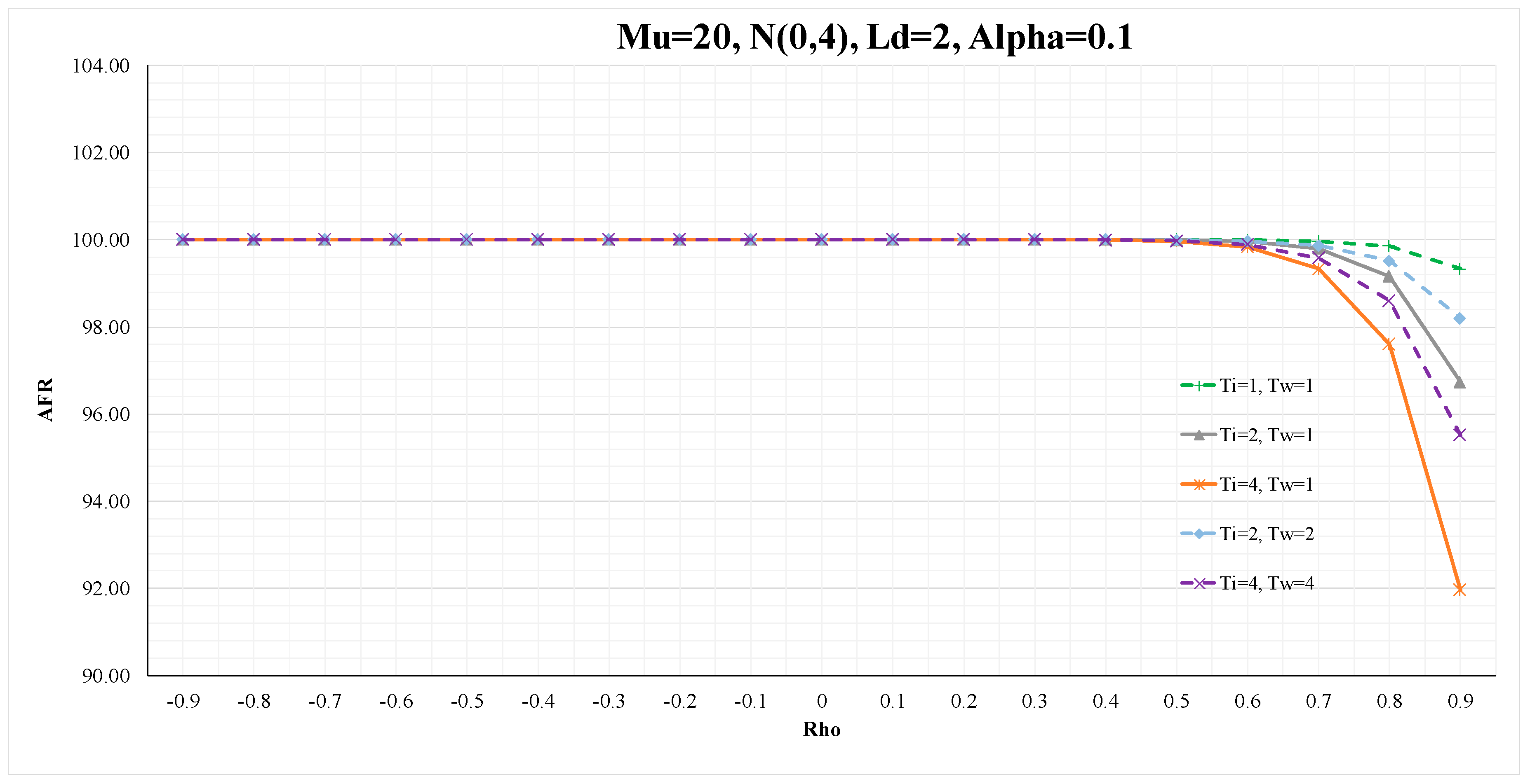
The impact of on AFR under the classical OUT policy is shown in Figure 6. The results indicate that AFR is not affected by the change of when the demand is negatively correlated, regardless of the level of Ld and . Similarly, the AFR is not affected by the change of for the i.i.d and slightly positive correlation demand. However, for the medium and highly positively correlated demand, AFR decreases as increases and that the reduction in AFR will be more for longer lead-time. Furthermore, at this demand structure, the selection of the smoothing parameters of the generalized OUT policy may lead to higher reduction in AFR (see Figure 7). This can be explained by the increase of NSA under such operating conditions as shown above. The results imply that the trade-off between order smoothing and amplification of net stock should be studied carefully when the demand is positively correlated. The higher order smoothing, the higher the safety stock needed to achieve a desired fill rate. Furthermore, the results confirm that the smoothing OUT policy is highly recommended for the negatively correlated demand as it can mitigate/eliminate the bullwhip effect without affecting the inventory performance measures (NSA and AFR) under such demand conditions.
5. Experimental Design and Analysis
The characterization results have shown that the demand correlation affects the supply chain performance and that its effect varies with the operating conditions: the lead-time (Ld), the ordering policy parameters (Ti and Tw), and the forecasting parameter (). The results have also revealed that such effects vary with the demand correlation level. To complement the characterization results, a statistically designed experiment is conducted to identify the most important factors and their interactions that significantly affect the studied three performance measures (OVR, NSA, AFR). Furthermore, the experimental design approach facilitates the statistical analysis of the simulation results, thus allowing to identify the statistically significant factors and interactions, and pointing out their relative importance with respect to the different performance measures.
5.1. Investigated Factors
A factorial design approach is considered to investigate the impact of positively correlated demand () with lead-time (Ld), forecasting parameter (), and ordering policy parameters (Ti and Tw) on the three measures of performance, OVR, NSA, and AFR. The investigated factors and their levels are summarized in Table 5, where two levels are considered for each of the five factors.
In this experiment, we consider only the case of positively correlated demand since it is the most commonly known in real applications [15,35]. Moreover, the characterization results have shown complex interactions between the operational parameters when the demand is positively correlated. In particular, the two levels of the autocorrelation parameter ‘Rho’ are selected to be within 0.3 and 0.7, where the correlated demand becomes nonstationary as Rho gets closer to one. Furthermore, the correlated demand in real supply chains is usually within Rho lower than 0.7 [17,20]. The levels of Ld, ‘Alpha’, Ti, and Tw are selected considering the used ranges in related studies [23,42]. Moreover, the low levels of both Ti and Tw are set to one in order to consider the impact of transforming from the classical OUT policy (Ti = Tw = 1) to the generalized OUT policy in this experiment. A full factorial design is run in which all possible combinations of the factors levels are investigated, resulting in 32 simulation scenarios. For each scenario, the simulation model is run for five replications with a simulation run length of 100,000 periods, and a warm-up of 5000 periods, to estimate the performance measures. The estimated performance measures (average responses) for the 32 simulation scenarios are presented in Table 6.
5.2. Results Analysis
An ANOVA study is conducted to investigate the statistical significance of the key factors and their interactions that impact the three performance measures. ANOVA results are presented in terms of the regression coefficients for a single order model (including the two-way interactions only), and the interaction plots. The regression coefficients tables given in Table 7, Table 8 and Table 9 convey the same information in the classical ANOVA tables in addition to effect magnitudes of the factors and their interactions.
The ANOVA results indicate that most of the investigated factors and their interactions have significant impact statistically on OVR and NSA (see Table 8 and Table 9). The investigated factors have similar impacts on both OVR and NSA. In particular, the direction of the change in response is the same for the main and interaction effects (see Figure 8, Figure 9 and Figure 10). Therefore, we present the analysis of the ANOVA results for both OVR and NSA, followed by a separate section for the analysis of ANOVA results of AFR.
5.2.1. Impact of Factors on OVR and NSA
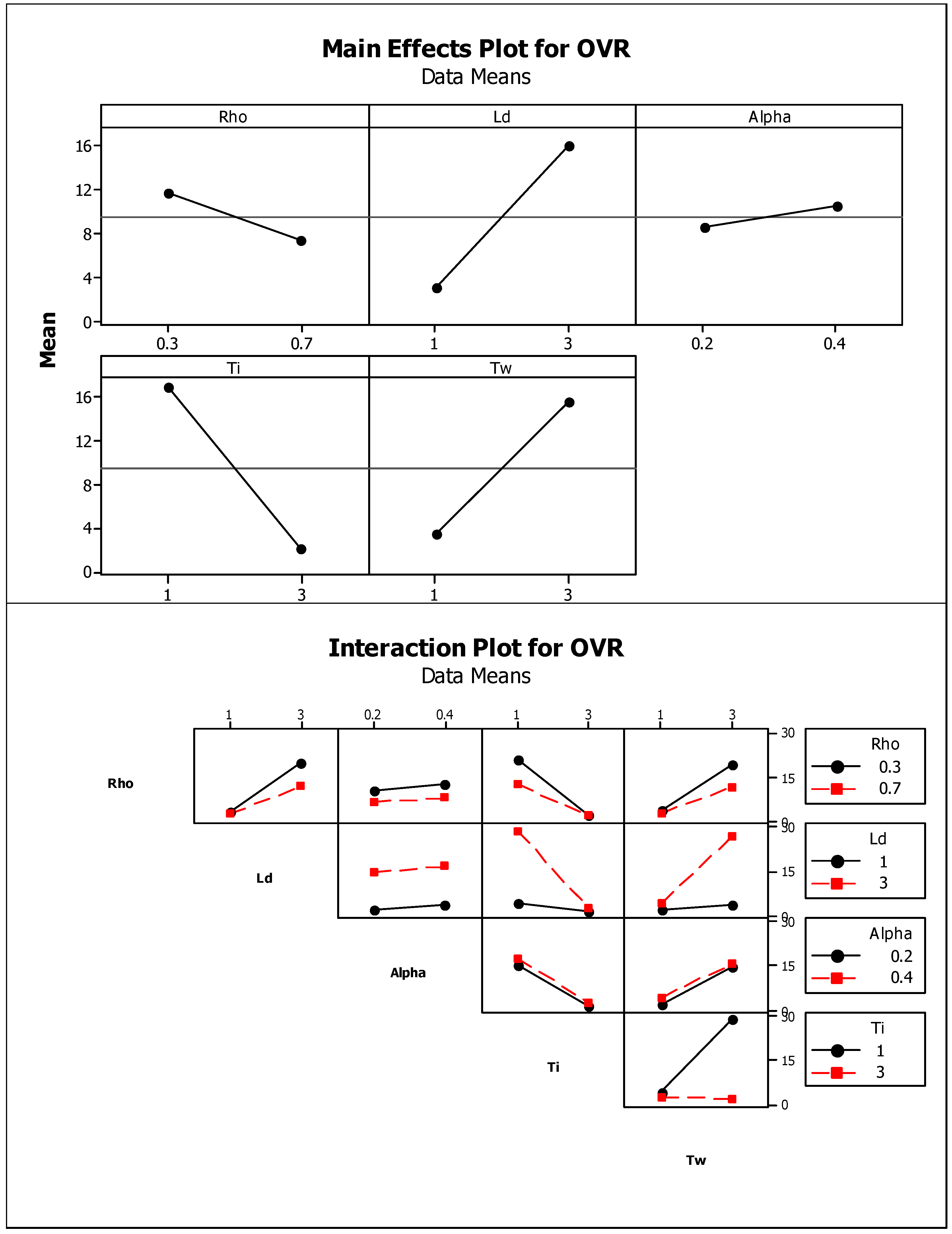
The ANOVA results confirm that the autocorrelation parameter (Rho) has a notable significant impact on OVR and NSA such that they both decrease as Rho increases (see Table 8 and Table 9). This can be clearly observed in the main effect plots shown in Figure 8 and Figure 9. Furthermore, the interaction effect plots show that the OVR and NSA measures are more sensitive to Rho under the classical OUT policy (Ti = 1) (see Figure 8 and Figure 9). However, this sensitivity decreases under the smoothing OUT (Ti > 1). In addition, it can be observed that the impact of Rho is substantial for long lead-times. This has also been shown in the characterization results for a wider range of Rho. The effect of Rho is almost independent of Alpha as can be revealed from the interaction plots. In general, the interaction effect plots indicate that both measures are less sensitive to changes in Rho value when Ti is large, Tw is small, and Ld is short.
Most importantly, the results show that the two smoothing parameters of the generalized OUT policy have the largest effects on both OVR and NSA. The previous research has assumed that both parameters are equal (Ti = Tw) and therefore their results confirm that higher levels of the smoothing parameter are of significant impact on the reduction/elimination of the bullwhip effect [28]. However, the analysis of the main effect plots suggests to select Ti = 3 (high) and Tw = 1 (low) for smaller OVR and NSA under the positively correlated demand. Furthermore, analyzing the interaction effect plots suggests that the combination of Ti = 3 and Tw = 1 also offers the least interaction between Ti and Tw. This confirms that the unmatched case of the smoothing parameters outperforms the matched case. The interaction of the smoothing parameters with the other operational parameters are statistically significant. At low level of Ld (Ld = 1), the OVR and NSA are not affected by the choice of Ti or Tw. However, long lead times (Ld = 3) favors large value of Ti (Ti = 3) and smaller value of Tw (Tw = 1). Low correlated demand (Rho = 0.3) also suggests large Ti and smaller Tw values to decrease OVR. At high correlation parameter (Rho = 0.7), these plots suggest that smaller value of Alpha and Ld, and OUT policy of Ti = 3 and Tw = 1 offers best performance. Therefore, it can be argued that the proper settings of Ti and Tw are of essential importance to control the variance amplification in supply chains with correlated demand.
The lead-time has one of the largest effects on OVR and NSA. However, the effect of lead-time can be counteracted by the proper selection of the ordering policy parameters as indicated above. The forecasting parameter (Alpha), in general, has the least impact on OVR and NSA. Its effect is almost independent (no interaction) of the levels of the other factors. This is evident also from the regression coefficients table, where all the interactions between Alpha and the other factors are insignificant.
5.2.2. Impact of Factors on AFR
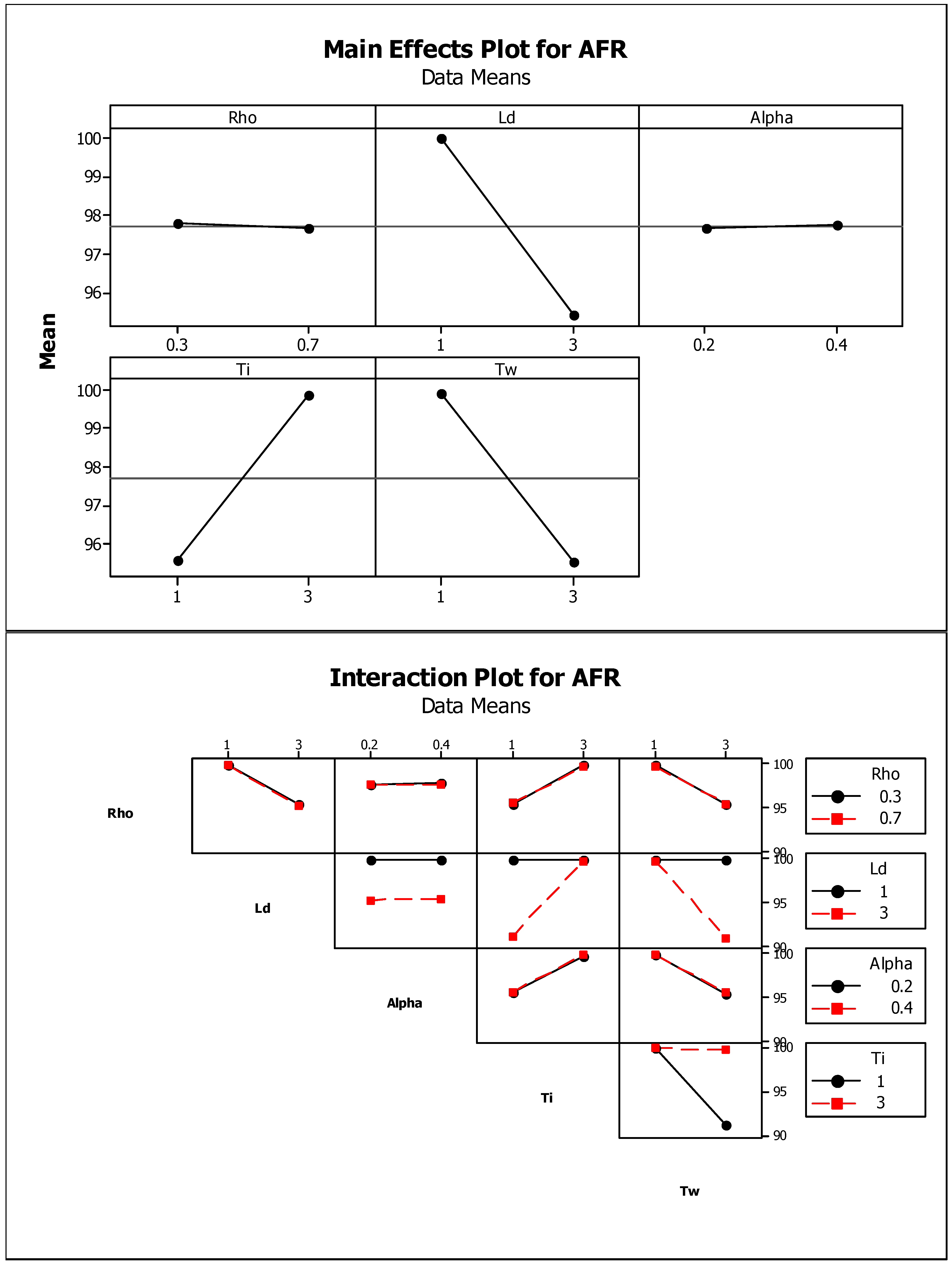
The main and interaction effects plots show that the fill rate is almost insensitive to correlation and forecasting parameters (see Figure 10). This is also evident from the related ANOVA results in Table 9. Changes in AFR are between 95% to 100% as the other factors (Ld, Ti, Tw) are varied in levels. Higher AFR values favor low Ld, high Ti, and low Tw. This policy is clearly similar to what is recommended for OVR and NSA measures.
6. Conclusions
Supply chains face the variance amplification in replenishment orders and inventory levels, leading to severe inefficiencies at all supply chain partners, such as increased production and inventory costs, and decreased serviceability. Therefore, variability need to be controlled to sustain economic and planned performance of a supply chain. In this regard, extensive modeling studies have been performed to analyze the variance amplification in supply chains while assuming i.i.d demands. Most of the previous studies have investigated the variance amplification in supply chain models that adopt the classical OUT policy, and permit return orders. These studies also have relied upon analytical modeling approaches, and therefore they analyzed the bullwhip effect only. Although supply chains that are subjected to correlated demand are common in reality, not enough attention is devoted to study their characterization and operational performance.
This research has adopted a simulation modeling approach in order to investigate the variance amplification and service level (average fill rate) in a supply chain that faces AR(1) demand, employs the generalized OUT policy, and restricts returns. The generalized OUT policy is a modified version of the classical OUT policy that can be adapted to allow order smoothing and thus mitigating and even eliminating the bullwhip effect. We utilize a simulation model to investigate the impact of correlated demand on order variance ratio (OVR), net stock amplification ratio (NSA), and average fill rate (AFR), under different operating conditions.
The characterization results for OVR and NSA under the classical OUT policy are consistent with the results reported in the literature. Exceptionally, the behavior of OVR over the negatively correlated demand is different from the previous research, due to the different modeling assumption of the allowance of returns. In particular, the results imply that applying the supply chain models that permits return orders will overestimate OVR for the supply chains that restrict returns. Therefore, supply chain practitioners will be misguided if they apply the existing analytical models to estimate the bullwhip effect for the negatively correlated demand. Existing analytical models should be revised to include the proper assumptions that are proved to have significant impact on the estimation of supply chain response.
The characterization results also reveal that the generalized OUT policy should be adopted with the correlated demand since its smoothing parameters can be tuned to produce better OVR and NSA without affecting the service level (AFR). For the negatively correlated demand, the best OVR, NSA, and AFR favors the generalized OUT policy with the matched smoothing parameters (Ti = Tw > 1). The generalized OUT policy can also be utilized to avoid the bullwhip effect (OVR) for both the i.i.d and positively correlated demand. The characterization results are complemented with a factorial design study that focused only on the positively correlated demand and the other operational parameters. The results confirmed that the ordering policy parameters and their interactions have the largest impact on the performance measures. In particular, the results have indicated that the unmatched smoothing parameters are more suitable than the matched settings for the positively correlated demand. The proper settings of the smoothing parameters will alleviate the impact of the lead-time and demand correlation on the performance measures.
This research provides useful managerial recommendations to control the variance amplification in supply chains with AR(1) demand. Supply chain managers have to identify the demand characteristics and determine the performance measures that they need to improve. If the demand is independent or correlated and the objective is to avoid the bullwhip effect, the managers are recommended to use the generalized OUT policy with the proper smoothing parameters according to the demand characteristics. The matched smoothing parameters (Ti = Tw > 1) are recommended for the negatively correlated or independent demand, while the unmatched settings (Ti > Tw) are preferred for the positively correlated demand. These recommended settings provide good inventory performance that can eliminate or minimize the bullwhip effect without affecting the inventory performance. This should lead to considerable savings in supply chain costs while achieving the desired service level, and thus sustaining the economic and planned performance of supply chains. However, managers need to keep track of inventory performance if they apply the generalized OUT policy with the positively correlated demand since it may affect net stock variability and service level. They also need to avoid the generalized OUT policy if inventory performance is their target measure. Moreover, for correlated demand, managers are recommended to trace the long-term average of the AR(1) demand process and use it as their demand forecast for every time period. When the demand is highly correlated, other responsive forecasting methods should be selected, and managers are advised to counteract the impact of lead-time through tuning the ordering policy parameters. These managerial implications are essential to achieve the techno-economic sustainability of supply chains with correlated demand.
For future research, forecasting methods other than the most industrially popular methods should be investigated, such as the time series forecasting methods and new adaptive forecasting methods that can comply with the nature of correlated demand. Also, the development of new ordering policies that cope with correlated demand is an interesting future research direction. The variance amplification under mixed and higher order correlated demand processes, such as ARIMA models and its variants, need to be characterized. The optimization of the forecasting and ordering policy parameters under correlated demand should be considered in future work. In general, performance of multi-echelon supply chains under correlated demand conditions is a highly viable research area of practical importance.
Author Contributions
Conceptualization, A.S., M.A.S. and G.D.G.; methodology, A.S. and M.A.S.; software, A.S., G.D.G. and R.P.; validation, A.S. and M.A.S.; formal analysis, A.S. and M.A.S.; investigation, A.S., M.A.S. and G.D.G.; resources, G.D.G. and R.P.; data curation, A.S., G.D.G. and R.P.; writing—original draft preparation, A.S.; writing—review and editing, A.S., M.A.S. and R.P.; visualization, A.S., G.D.G. and R.P.; supervision, M.A.S.; project administration, A.S., M.A.S. and G.D.G; funding acquisition, G.D.G. and R.P. All authors have read and agreed to the published version of the manuscript.
Funding
This research received no external funding.
Conflicts of Interest
The authors declare no conflict of interest.
References
- Priore, P.; Ponte, B.; Rosillo, R.; de la Fuente, D. Applying machine learning to the dynamic selection of replenishment policies in fast-changing supply chain environments. Int. J. Prod. Res. 2019, 57, 3663–3677. [Google Scholar] [CrossRef]
- Costantino, F.; Di Gravio, G.; Patriarca, R.; Petrella, L. Spare parts management for irregular demand items. Omega (UK) 2018, 81, 57–66. [Google Scholar] [CrossRef]
- Pastore, E.; Alfieri, A.; Zotteri, G. An empirical investigation on the antecedents of the bullwhip effect: Evidence from the spare parts industry. Int. J. Prod. Econ. 2019, 209, 121–133. [Google Scholar] [CrossRef]
- Alvarado-Vargas, M.J.; Kelley, K.J. Bullwhip severity in conditions of uncertainty: Regional vs global supply chain strategies. Int. J. Emerg. Mark. 2019, 15, 131–148. [Google Scholar] [CrossRef]
- Lambrecht, M.R.; Disney, S.M. On replenishment rules, forecasting, and the bullwhip effect in supply chains. Found. Trends Technol. Inf. Oper. Manag. 2008, 2, 1–80. [Google Scholar]
- Huang, J.; Shuai, Y.; Liu, Q.; Zhou, H.; He, Z. Synergy Degree Evaluation Based on Synergetics for Sustainable Logistics Enterprises. Sustainability 2018, 10, 2187. [Google Scholar] [CrossRef] [Green Version]
- Qu, Y.; Yu, Y.; Appolloni, A.; Li, M.; Liu, Y. Measuring Green Growth Efficiency for Chinese Manufacturing Industries. Sustainability 2017, 9, 637. [Google Scholar] [CrossRef] [Green Version]
- Wang, X.; Disney, S.M. The bullwhip effect: Progress, trends and directions. Eur. J. Oper. Res. 2016, 250, 691–701. [Google Scholar] [CrossRef] [Green Version]
- Shaban, A.; Costantino, F.; Di Gravio, G.; Tronci, M. Coordinating of multi-echelon supply chains through the generalized (R, S) policy. Simulation 2020. [Google Scholar] [CrossRef]
- Dejonckheere, J.; Disney, S.M.; Lambrecht, M.R.; Towill, D.R. Measuring and avoiding the bullwhip effect: A control theoretic approach. Eur. J. Oper. Res. 2003, 147, 567–590. [Google Scholar] [CrossRef]
- Dejonckheere, J.; Disney, S.; Lambrecht, M.; Towill, D. The impact of information enrichment on the Bullwhip effect in supply chains: A control engineering perspective. Eur. J. Oper. Res. 2004, 153, 727–750. [Google Scholar] [CrossRef]
- Costantino, F.; Di Gravio, G.; Shaban, A.; Tronci, M. A real-time SPC inventory replenishment system to improve supply chain performances. Expert Syst. Appl. 2015, 42, 1665–1683. [Google Scholar] [CrossRef]
- Dominguez, R.; Ponte, B.; Cannella, S.; Framinan, J.M. On the dynamics of closed-loop supply chains with capacity constraints. Comput. Ind. Eng. 2019, 128, 91–103. [Google Scholar] [CrossRef]
- Lee, H.; Padmanabhan, V.; Whang, S. The Bullwhip Effect in Supply Chains. Sloan Manag. Rev. 1997, 38, 93–102. [Google Scholar] [CrossRef]
- Lee, H.L.; So, K.C.; Tang, C.S. The Value of Information Sharing in a Two-Level Supply Chain. Manag. Sci. 2000, 46, 626–643. [Google Scholar] [CrossRef] [Green Version]
- Mahajan, S.; Venugopal, V. Value of Information Sharing and Lead Time Reduction in a Supply Chain with Autocorrelated Demand. Technol. Oper. Manag. 2011, 2, 39–49. [Google Scholar] [CrossRef]
- Boute, R.N.; Disney, S.M.; Lambrecht, M.; Van Houdt, B. Coordinating Lead-Time and Safety Stock Decisions in a Two-Echelon Supply Chain with Autocorrelated Consumer Demand. SSRN Electron. J. 2020. [Google Scholar] [CrossRef] [Green Version]
- Michna, Z.; Disney, S.M.; Nielsen, P. The impact of stochastic lead times on the bullwhip effect under correlated demand and moving average forecasts. Omega 2019, 93, 102033. [Google Scholar] [CrossRef] [Green Version]
- Tai, P.D.; Duc, T.T.H.; Buddhakulsomsiri, J. Measure of bullwhip effect in supply chain with price-sensitive and correlated demand. Comput. Ind. Eng. 2019, 127, 408–419. [Google Scholar] [CrossRef]
- Erkip, N.; Hausman, W.H.; Nahmias, S. Optimal Centralized Ordering Policies in Multi-Echelon Inventory Systems with Correlated Demands. Manag. Sci. 1990, 36, 381–392. [Google Scholar] [CrossRef]
- Luong, H.T. Measure of bullwhip effect in supply chains with autoregressive demand process. Eur. J. Oper. Res. 2007, 180, 1086–1097. [Google Scholar] [CrossRef]
- Duc, T.T.H.; Luong, H.T.; Kim, Y.-D. A measure of bullwhip effect in supply chains with a mixed autoregressive-moving average demand process. Eur. J. Oper. Res. 2008, 187, 243–256. [Google Scholar] [CrossRef]
- Hussain, M.; Shome, A.; Lee, D.M. Impact of forecasting methods on variance ratio in order-up-to level policy. Int. J. Adv. Manuf. Technol. 2012, 59, 413–420. [Google Scholar] [CrossRef]
- Chatfield, D.C.; Pritchard, A.M. Returns and the bullwhip effect. Transp. Res. Part E Logist. Transp. Rev. 2013, 49, 15–175. [Google Scholar] [CrossRef]
- Dominguez, R.; Cannella, S.; Framinan, J.M. On returns and network configuration in supply chain dynamics. Transp. Res. Part. E Logist. Transp. Rev. 2015, 73, 152–167. [Google Scholar] [CrossRef]
- Shaban, A.; Shalaby, M.A. Modeling and optimizing of variance amplification in supply chain using response surface methodology. Comput. Ind. Eng. 2018, 120, 392–400. [Google Scholar] [CrossRef]
- Jakšič, M.; Rusjan, B. The effect of replenishment policies on the bullwhip effect: A transfer function approach. Eur. J. Oper. Res. 2008, 184, 946–961. [Google Scholar] [CrossRef]
- Disney, S.M.; Farasyn, I.; Lambrecht, M.; Towill, D.R.; de Velde, W. Van Taming the bullwhip effect whilst watching customer service in a single supply chain echelon. Eur. J. Oper. Res. 2006, 173, 151–172. [Google Scholar] [CrossRef]
- Zotteri, G. An empirical investigation on causes and effects of the Bullwhip-effect: Evidence from the personal care sector. Int. J. Prod. Econ. 2013, 143, 489–498. [Google Scholar] [CrossRef]
- Klug, F. The Internal Bullwhip Effect in Car Manufacturing. Int. J. Prod. Res. 2013, 51, 303–322. [Google Scholar] [CrossRef]
- Chiang, C.-Y.; Lin, W.T.; Suresh, N.C. An empirically-simulated investigation of the impact of demand forecasting on the bullwhip effect: Evidence from U.S. auto industry. Int. J. Prod. Econ. 2016, 177, 53–65. [Google Scholar] [CrossRef]
- Sterman, J.D. Modeling Managerial Behavior: Misperceptions of Feedback in a Dynamic Decision Making Experiment. Manag. Sci. 1989, 35, 321–339. [Google Scholar] [CrossRef] [Green Version]
- Shovityakool, P.; Jittam, P.; Sriwattanarothai, N.; Laosinchai, P. A Flexible Supply Chain Management Game. Simul. Gaming 2019, 50, 461–482. [Google Scholar] [CrossRef]
- Wu, D.Y.; Katok, E. Learning, communication, and the bullwhip effect. J. Oper. Manag. 2006, 24, 839–850. [Google Scholar] [CrossRef]
- Lee, H.L.; Padmanabhan, V.; Whang, S. Information Distortion in a Supply Chain: The Bullwhip Effect. Manag. Sci. 1997, 43, 546–558. [Google Scholar] [CrossRef]
- Nienhaus, J.; Ziegenbein, A.; Duijts, C. How human behaviour amplifies the bullwhip effect—A study based on the beer distribution game online. Prod. Plan. Control. 2006, 17, 547–557. [Google Scholar] [CrossRef]
- Chen, F.; Ryan, J.K.; Simchi-Levi, D. The Impact of Exponential Smoothing Forecasts on the Bullwhip Effect. Nav. Res. Logist. 2000, 47, 269. [Google Scholar] [CrossRef]
- Kim, J.G.; Chatfield, D.; Harrison, T.P.; Hayya, J.C. Quantifying the bullwhip effect in a supply chain with stochastic lead time. Eur. J. Oper. Res. 2006, 173, 617–636. [Google Scholar] [CrossRef]
- Disney, S.M.; Towill, D.R. On the bullwhip and inventory variance produced by an ordering policy. Omega 2003, 31, 157–167. [Google Scholar] [CrossRef]
- Chatfield, D.C.; Kim, J.G.; Harrison, T.P.; Hayya, J.C. The Bullwhip Effect-Impact of Stochastic Lead Time, Information Quality, and Information Sharing: A Simulation Study. Prod. Oper. Manag. 2004, 13, 340–353. [Google Scholar] [CrossRef]
- Shaban, A.; Costantino, F.; Di Gravio, G.; Tronci, M. A new efficient collaboration model for multi-echelon supply chains. Expert Syst. Appl. 2019, 128, 54–66. [Google Scholar] [CrossRef]
- Cannella, S. Order-Up-To policies in Information Exchange supply chains. Appl. Math. Model. 2014, 38, 5553–5561. [Google Scholar] [CrossRef]
- Jaipuria, S.; Mahapatra, S.S. An improved demand forecasting method to reduce bullwhip effect in supply chains. Expert Syst. Appl. 2014, 41, 2395–2408. [Google Scholar] [CrossRef]
- Hussain, M.; Saber, H. Exploring the bullwhip effect using simulation and Taguchi experimental design. Int. J. Logist. Res. Appl. 2012, 15, 231–249. [Google Scholar] [CrossRef]
- Dominguez, R.; Cannella, S.; Barbosa-Póvoa, A.P.; Framinan, J.M. OVAP: A strategy to implement partial information sharing among supply chain retailers. Transp. Res. Part E Logist. Transp. Rev. 2018, 110, 122–136. [Google Scholar] [CrossRef]
- Zhang, X. The impact of forecasting methods on the bullwhip effect. Int. J. Prod. Econ. 2004, 88, 15–27. [Google Scholar] [CrossRef]
- Luong, H.; Phien, N. Measure of bullwhip effect in supply chains: The case of high order autoregressive demand process. Eur. J. Oper. Res. 2007, 183, 197–209. [Google Scholar] [CrossRef]
- Sirikasemsuk, K.; Luong, H.T. Measure of bullwhip effect in supply chains with first-order bivariate vector autoregression time-series demand model. Comput. Oper. Res. 2017, 78, 59–79. [Google Scholar] [CrossRef]
- Chandra, C.; Grabis, J. Application of multi-steps forecasting for restraining the bullwhip effect and improving inventory performance under autoregressive demand. Eur. J. Oper. Res. 2005, 166, 337–350. [Google Scholar] [CrossRef]
- Chen, F.; Drezner, Z.; Ryan, J.K.; Simchi-Levi, D. Quantifying the Bullwhip Effect in a Simple Supply Chain: The Impact of Forecasting, Lead Times, and Information. Manag. Sci. 2000, 46, 436–443. [Google Scholar] [CrossRef] [Green Version]
- Ma, Y.; Wang, N.; Che, A.; Huang, Y.; Xu, J. The bullwhip effect on product orders and inventory: A perspective of demand forecasting techniques. Int. J. Prod. Res. 2013, 51, 281–302. [Google Scholar] [CrossRef] [Green Version]
- Campuzano-Bolarín, F.; Frutos, A.G.; Ruiz Abellón, M.D.C.; Lisec, A. Alternative Forecasting Techniques that Reduce the Bullwhip Effect in a Supply Chain: A Simulation Study. Prsomet–Traffic Transp. 2013, 25, 177–188. [Google Scholar] [CrossRef] [Green Version]
- Costantino, F.; Di Gravio, G.; Shaban, A.; Tronci, M. SPC forecasting system to mitigate the bullwhip effect and inventory variance in supply chains. Expert Syst. Appl. 2015, 42, 1773–1787. [Google Scholar] [CrossRef]
- Bandyopadhyay, S.; Bhattacharya, R. A generalized measure of bullwhip effect in supply chain with ARMA demand process under various replenishment policies. Int. J. Adv. Manuf. Technol. 2013, 68, 963–979. [Google Scholar] [CrossRef]
- Gaalman, G.; Disney, S. On bullwhip in a family of order-up-to policies with ARMA (2, 2) demand and arbitrary lead-times. Int. J. Prod. Econ. 2009, 121, 454–463. [Google Scholar] [CrossRef]
- Pacheco, E.D.O.; Cannella, S.; Lüders, R.; Barbosa-Povoa, A.P. Order-up-to-level policy update procedure for a supply chain subject to market demand uncertainty. Comput. Ind. Eng. 2017, 113, 347–355. [Google Scholar] [CrossRef]
- Costantino, F.; Di Gravio, G.; Shaban, A.; Tronci, M. The impact of information sharing and inventory control coordination on supply chain performances. Comput. Ind. Eng. 2014, 76, 292–306. [Google Scholar] [CrossRef]
- Patriarca, R.; Costantino, F.; Di Gravio, G.; Tronci, M. Inventory optimization for a customer airline in a Performance Based Contract. J. Air Transp. Manag. 2016, 57, 206–216. [Google Scholar] [CrossRef]
Figure 1.
Different simulated instances of first order autoregressive AR(1) demand process.

Figure 2.
The impact of on OVR under classical OUT policy for Ld = 2 and Ld = 4.


Figure 3.
The impact of the ordering policy parameters on OVR.

Figure 4.
The impact of on NSA under the classical OUT policy (Ti = Tw = 1).


Figure 5.
The impact of the ordering policy parameters (Ti and Tw) on NSA.

Figure 6.
The impact of on AFR under the classical order-up-to (OUT) policy (Ti = Tw = 1).

Figure 7.
The impact of the ordering policy parameters on average fill rate (AFR).

Figure 8.
The effects of the investigated factors and their interactions on OVR.

Figure 9.
The effects of the investigated factors and their interactions on NSA.

Figure 10.
The main and interaction effects of the investigated factors on AFR.


Table 1.
Closed form expressions for order variance ratio (OVR) and net stock amplification ratio (NSA).
Table 1.
Closed form expressions for order variance ratio (OVR) and net stock amplification ratio (NSA).
| Measure | Mathematical Expressions |
|---|---|
| Chen, Ryan, and Simchi-Levi [37] | |
| Disney et al. [28] | |
Table 2.
Simulation model validation for OVR.
| OVR | |||||||
|---|---|---|---|---|---|---|---|
| −0.9 | −0.6 | −0.3 | 0 | 0.3 | 0.6 | 0.9 | |
| Analytical * | 2.0166 | 2.0062 | 1.9913 | 1.9684 | 1.9286 | 1.8421 | 1.5097 |
| Simulation Model | 2.0170 | 2.0325 | 2.0280 | 2.0103 | 1.9673 | 1.8710 | 1.5206 |
Table 3.
Simulation model validation for NSA.
| NSA | |||||||
|---|---|---|---|---|---|---|---|
| −0.9 | −0.6 | −0.3 | 0 | 0.3 | 0.6 | 0.9 | |
| Analytical * | 1.0200 | 1.3200 | 1.9800 | 3.0000 | 4.3800 | 6.1200 | 8.2200 |
| Simulation Model | 1.0282 | 1.3434 | 2.0012 | 3.0018 | 4.3542 | 6.0761 | 8.1940 |
* Disney et al. [28].
Table 4.
The OVR under highly negative correlation demand.
| Variance Measure | |||||
|---|---|---|---|---|---|
| −0.5 | −0.6 | −0.7 | −0.8 | −0.9 | |
| DV | 5.4001 | 6.3104 | 7.9062 | 11.1886 | 21.2177 |
| = 0.4) | 45.1737 | 53.4232 | 66.9546 | 91.6913 | 145.9274 |
| = 0.4) | 8.3653 | 8.4659 | 8.4686 | 8.1952 | 6.8782 |
| = 0.4) | 77.4508 | 90.0306 | 109.3083 | 140.8079 | 200.0207 |
| = 0.4) | 14.3425 | 14.2672 | 13.8258 | 12.5855 | 9.4281 |
Table 5.
Investigated factors and their levels.
| Factors | Levels | |
|---|---|---|
| Low (−1) | High (+1) | |
| ) | 0.3 | 0.7 |
| Ld | 1 | 3 |
| ) | 0.2 | 0.4 |
| Ti | 1 | 3 |
| Tw | 1 | 3 |
Table 6.
Full factorial design and estimated performance measures.
| Run | Factors | Performance Measures | ||||||
|---|---|---|---|---|---|---|---|---|
| Rho | Ld | Alpha | Ti | Tw | OVR | NSA | AFR (%) | |
| 1 | 0.3 | 1 | 0.2 | 1 | 1 | 2.5160 | 3.6273 | 100.00 |
| 2 | 0.3 | 1 | 0.2 | 1 | 3 | 5.3611 | 6.4040 | 100.00 |
| 3 | 0.3 | 1 | 0.2 | 3 | 1 | 1.0053 | 4.0964 | 100.00 |
| 4 | 0.3 | 1 | 0.2 | 3 | 3 | 0.9111 | 4.3437 | 100.00 |
| 5 | 0.3 | 1 | 0.4 | 1 | 1 | 4.6327 | 4.7139 | 100.00 |
| 6 | 0.3 | 1 | 0.4 | 1 | 3 | 9.2888 | 9.8288 | 99.99 |
| 7 | 0.3 | 1 | 0.4 | 3 | 1 | 2.1224 | 3.6417 | 100.00 |
| 8 | 0.3 | 1 | 0.4 | 3 | 3 | 1.5111 | 4.2698 | 100.00 |
| 9 | 0.3 | 3 | 0.2 | 1 | 1 | 3.9103 | 9.6054 | 99.99 |
| 10 | 0.3 | 3 | 0.2 | 1 | 3 | 66.9747 | 202.1584 | 81.70 |
| 11 | 0.3 | 3 | 0.2 | 3 | 1 | 2.1973 | 7.9704 | 100.00 |
| 12 | 0.3 | 3 | 0.2 | 3 | 3 | 1.2658 | 9.6863 | 99.99 |
| 13 | 0.3 | 3 | 0.4 | 1 | 1 | 8.7397 | 13.1250 | 99.95 |
| 14 | 0.3 | 3 | 0.4 | 1 | 3 | 66.3925 | 200.7926 | 82.62 |
| 15 | 0.3 | 3 | 0.4 | 3 | 1 | 6.7739 | 8.9613 | 99.99 |
| 16 | 0.3 | 3 | 0.4 | 3 | 3 | 2.3617 | 10.5368 | 99.98 |
| 17 | 0.7 | 1 | 0.2 | 1 | 1 | 2.1196 | 3.7074 | 100.00 |
| 18 | 0.7 | 1 | 0.2 | 1 | 3 | 3.8702 | 4.8929 | 100.00 |
| 19 | 0.7 | 1 | 0.2 | 3 | 1 | 1.1697 | 6.5795 | 99.98 |
| 20 | 0.7 | 1 | 0.2 | 3 | 3 | 1.3344 | 6.3646 | 99.98 |
| 21 | 0.7 | 1 | 0.4 | 1 | 1 | 3.2204 | 4.0068 | 100.00 |
| 22 | 0.7 | 1 | 0.4 | 1 | 3 | 6.0879 | 6.8081 | 99.97 |
| 23 | 0.7 | 1 | 0.4 | 3 | 1 | 1.7462 | 4.5801 | 100.00 |
| 24 | 0.7 | 1 | 0.4 | 3 | 3 | 1.7977 | 5.2627 | 99.99 |
| 25 | 0.7 | 3 | 0.2 | 1 | 1 | 3.1573 | 12.5909 | 99.65 |
| 26 | 0.7 | 3 | 0.2 | 1 | 3 | 38.1882 | 122.2211 | 82.68 |
| 27 | 0.7 | 3 | 0.2 | 3 | 1 | 1.6287 | 14.1497 | 99.51 |
| 28 | 0.7 | 3 | 0.2 | 3 | 3 | 1.8007 | 16.5540 | 99.21 |
| 29 | 0.7 | 3 | 0.4 | 1 | 1 | 5.7269 | 13.9211 | 99.51 |
| 30 | 0.7 | 3 | 0.4 | 1 | 3 | 39.6230 | 127.7397 | 82.79 |
| 31 | 0.7 | 3 | 0.4 | 3 | 1 | 3.7065 | 11.2083 | 99.77 |
| 32 | 0.7 | 3 | 0.4 | 3 | 3 | 2.6806 | 15.5031 | 99.33 |
Table 7.
Estimated Effects and Coefficients for OVR (coded units).
| Term | Effect | Coef | SE Coef | T | P |
|---|---|---|---|---|---|
| Constant | 9.494 | 0.1451 | 65.44 | 0.000 | |
| Rho | −4.257 | −2.128 | 0.1451 | −14.67 | 0.000 |
| Ld | 12.902 | 6.451 | 0.1451 | 44.46 | 0.000 |
| Alpha | 1.813 | 0.906 | 0.1451 | 6.25 | 0.000 |
| Ti | −14.737 | −7.369 | 0.1451 | −50.79 | 0.000 |
| Tw | 12.192 | 6.096 | 0.1451 | 42.02 | 0.000 |
| Rho*Ld | −3.506 | −1.753 | 0.1451 | −12.08 | 0.000 |
| Rho*Alpha | −0.398 | −0.199 | 0.1451 | −1.37 | 0.173 |
| Rho*Ti | 3.971 | 1.986 | 0.1451 | 13.68 | 0.000 |
| Rho*Tw | −3.079 | −1.539 | 0.1451 | −10.61 | 0.000 |
| Ld*Alpha | 0.298 | 0.149 | 0.1451 | 1.03 | 0.307 |
| Ld*Ti | −11.55 | −5.775 | 0.1451 | −39.8 | 0.000 |
| Ld*Tw | 10.739 | 5.369 | 0.1451 | 37.01 | 0.000 |
| Alpha*Ti | −0.389 | −0.195 | 0.1451 | −1.34 | 0.182 |
| Alpha*Tw | −0.558 | −0.279 | 0.1451 | −1.92 | 0.057 |
| Ti*Tw | −13.028 | −6.514 | 0.1451 | −44.9 | 0.000 |
Table 8.
Estimated Effects and Coefficients for NSA (coded units).
| Term | Effect | Coef | SE Coef | T | P |
|---|---|---|---|---|---|
| Constant | 27.5 | 1.726 | 15.93 | 0.000 | |
| Rho | −7.98 | −3.99 | 1.726 | −2.31 | 0.022 |
| Ld | 44.6 | 22.3 | 1.726 | 12.92 | 0.000 |
| Alpha | 0.62 | 0.31 | 1.726 | 0.18 | 0.857 |
| Ti | −38.28 | −19.14 | 1.726 | −11.09 | 0.000 |
| Tw | 39.18 | 19.59 | 1.726 | 11.35 | 0.000 |
| Rho*Ld | −8.14 | −4.07 | 1.726 | −2.36 | 0.020 |
| Rho*Alpha | −0.38 | −0.19 | 1.726 | −0.11 | 0.914 |
| Rho*Ti | 11.32 | 5.66 | 1.726 | 3.28 | 0.001 |
| Rho*Tw | −9.85 | −4.93 | 1.726 | −2.85 | 0.005 |
| Ld*Alpha | 0.23 | 0.12 | 1.726 | 0.07 | 0.946 |
| Ld*Ti | −37.67 | −18.84 | 1.726 | −10.91 | 0.000 |
| Ld*Tw | 37.53 | 18.76 | 1.726 | 10.87 | 0.000 |
| Alpha*Ti | −1.34 | −0.67 | 1.726 | −0.39 | 0.698 |
| Alpha*Tw | 0.39 | 0.2 | 1.726 | 0.11 | 0.910 |
| Ti*Tw | −37.76 | −18.88 | 1.726 | −10.94 | 0.000 |
Table 9.
Estimated Effects and Coefficients for AFR (coded units).
| Term | Effect | Coef | SE Coef | T | P |
|---|---|---|---|---|---|
| Constant | 97.706 | 0.1791 | 545.67 | 0.000 | |
| Rho | −0.116 | −0.058 | 0.1791 | −0.32 | 0.746 |
| Ld | −4.576 | −2.288 | 0.1791 | −12.78 | 0.000 |
| Alpha | 0.077 | 0.038 | 0.1791 | 0.21 | 0.831 |
| Ti | 4.306 | 2.153 | 0.1791 | 12.02 | 0.000 |
| Tw | −4.381 | −2.19 | 0.1791 | −12.23 | 0.000 |
| Rho*Ld | −0.106 | −0.053 | 0.1791 | −0.3 | 0.767 |
| Rho*Alpha | −0.031 | −0.016 | 0.1791 | −0.09 | 0.931 |
| Rho*Ti | −0.158 | −0.079 | 0.1791 | −0.44 | 0.660 |
| Rho*Tw | 0.075 | 0.037 | 0.1791 | 0.21 | 0.835 |
| Ld*Alpha | 0.076 | 0.038 | 0.1791 | 0.21 | 0.831 |
| Ld*Ti | 4.307 | 2.154 | 0.1791 | 12.03 | 0.000 |
| Ld*Tw | −4.376 | −2.188 | 0.1791 | −12.22 | 0.000 |
| Alpha*Ti | −0.026 | −0.013 | 0.1791 | −0.07 | 0.942 |
| Alpha*Tw | 0.065 | 0.032 | 0.1791 | 0.18 | 0.857 |
| Ti*Tw | 4.287 | 2.143 | 0.1791 | 11.97 | 0.000 |
© 2020 by the authors. Licensee MDPI, Basel, Switzerland. This article is an open access article distributed under the terms and conditions of the Creative Commons Attribution (CC BY) license (http://creativecommons.org/licenses/by/4.0/).
Share and Cite
MDPI and ACS Style
Shaban, A.; Shalaby, M.A.; Di Gravio, G.; Patriarca, R. Analysis of Variance Amplification and Service Level in a Supply Chain with Correlated Demand. Sustainability 2020, 12, 6470. https://doi.org/10.3390/su12166470
AMA Style
Shaban A, Shalaby MA, Di Gravio G, Patriarca R. Analysis of Variance Amplification and Service Level in a Supply Chain with Correlated Demand. Sustainability. 2020; 12(16):6470. https://doi.org/10.3390/su12166470
Chicago/Turabian StyleShaban, Ahmed, Mohamed A. Shalaby, Giulio Di Gravio, and Riccardo Patriarca. 2020. "Analysis of Variance Amplification and Service Level in a Supply Chain with Correlated Demand" Sustainability 12, no. 16: 6470. https://doi.org/10.3390/su12166470
Note that from the first issue of 2016, this journal uses article numbers instead of page numbers. See further details here.