Multicriteria ABC Inventory Classification Using the Social Choice Theory

School of Management & Engineering, Nanjing University, Nanjing 210000, China
*
Author to whom correspondence should be addressed.
Sustainability 2020, 12(1), 182; https://doi.org/10.3390/su12010182
Submission received: 3 November 2019
/
Revised: 17 December 2019
/
Accepted: 20 December 2019
/
Published: 24 December 2019
(This article belongs to the Special Issue Inventory Management for Sustainable Industrial Operations)
Abstract
:The multicriteria ABC inventory classification has been widely adopted by organizations for the purpose of specifying, monitoring, and controlling inventory efficiently. It categorizes the items into three groups based on some certain criteria, such as inventory cost, part criticality, lead time, and commonality. There has been extensive research on such a problem, but few have considered that the judgments about criteria’s importance order usually exhibit a substantial degree of variability. In light of this, we propose a new methodology for handling the multicriteria ABC inventory classification problem using the social choice theory. Specifically, the pessimistic and optimistic results for all possible individual judgments are obtained in a closed-form manner, which are then balanced by the Hurwicz criterion with a “coefficient of optimism”. The CRITIC (Criteria Importance Through Intercriteria Correlation) method is used to aggregate the individual judgments into a collective choice, according to which the items are classified into Groups A, B, and C. Through a numerical experiment, we show that the proposed methodology not only considers all possible preferences among the criteria, but also generates flexible classification schemes.
1. Introduction
Inventory is a necessary evil in any organization engaged in production and sale. Every unit of inventory has an economic value and is considered an asset of the organization irrespective of where it is located or in which form it is available. Nevertheless, emissions caused by inventory and related warehousing activities have gained considerable attention from both the government and the public [1]. It is pointed out by Fichtinger [2] that those emissions are highly influenced by inventory management. Therefore, efficient inventory management is critical for reducing the environmental and social impacts of organizations while maintaining their revenues [3].
For organizations with a large number of stock keeping units (SKUs), it is time and money consuming to manage each SKU individually. A common solution is to categorize the SKUs into different groups with some logic for the purpose of managing in the same manner. In most of the organizations, inventory is categorized according to ABC analysis, which is performed based on the Pareto principle and detaches the “trivial many” from the “vital few”. The ABC inventory classification provides not only a mechanism to identify SKUs that significantly affect the overall inventory cost, but also a method to pinpoint different categories of inventory that require different management and control policies [4]. Generally speaking, it categorizes the SKUs into three groups based on the 80/20 principle: Group A (very important SKUs), Group B (moderately important SKUs), and Group C (relatively unimportant SKUs) [5]. The primary goal of ABC classification is to simplify the inventory management by means of determining stock control levels of each class [6]. Benefiting from the easy-to-understand and simple-to-implement features and the excellent performance in inventory management, ABC classification has been extensively utilized to improve the efficiency of inventory control [7].
The classification of SKUs into A, B, and C groups has been traditionally implemented based solely on one criterion, namely annual dollar usage (ADU) of the SKUs. This to a large extent reflects the principle that a small proportion of SKUs accounts for a majority of the dollar usage [8]. Nevertheless, there exist other criteria that indicate important considerations for management. Ramanathan [9] presented a summary of additional criteria that should been taken into account in ABC inventory classification: “inventory cost, part criticality, lead time, commonality, obsolescence, substitutability, number of requests for the item in a year, scarcity, durability, reparability, order size requirement, shockability, demand distribution, and stock-out penalty cost.” In addition, the individual judgments about the criteria’s importance order are usually different among decision makers [6], leading to different results of inventory classification. Each of the results may have some valuable advantages that cannot be ignored; thus, it is suggested to accept all possible results first and then aggregate them to generate a comprehensive score [10].
Therefore, the purpose of this study is to propose a new methodology, which takes into account all possible individual judgments about criteria’s importance rankings, for handling the multicriteria ABC inventory classification problem. Generally speaking, for each ranking, we first derive the pessimistic and optimistic results of individual judgments among the classification criteria in a closed-form. Secondly, we combine each pair of the extreme results into one index. The set of indices is finally combined together to classify the SKUs. The proposed methodology is applied to the data provided by Ramanathan [9]. Numerical results demonstrate the usefulness of the proposed methodology, that it is able to take into account all possible individual preferences on classification criteria.
Our paper also contributes to the existing research by using the social choice theory. In the presence of multiple individual judgments, social choice theory investigates how one designs or chooses a mechanism to summarize from a set of individual judgments over alternatives available to a society with those individuals into a collective or social judgment over those same alternatives [11,12]. The application of social choice theory to decision making has been performed in literature. Dyer and Miles [13] and Srdjevic [14] demonstrated the relationship between social choice theory and group decision making and used the proposed models for the Mariner Jupiter/Saturn 1977 project and water management, respectively. These papers in essence motivated our study that models various individual judgments and aggregates them from a collective choice viewpoint. In accordance with Diakoulaki et al. [15] and Rostamzadeh et al. [16], we chose to use the CRITIC (Criteria Importance Through Intercriteria Correlation) method.
The remainder of the paper is organized as follows. The literature related to our paper is discussed in Section 2. Section 3 describes the research problem. In Section 4, we present our methodology for implementing multicriteria ABC inventory classification, followed by an illustrative example in Section 5. We conclude in Section 6 by discussing the details of our methodology and suggestions for future research.
2. Literature Review
There has been extensive research where various operations research (OR) methods are developed to cope with the multicriteria ABC inventory classification problem.
An important branch makes full use of various optimization models. Ramanathan [9] proposed a weighted linear optimization model to classify SKUs in the presence of multiple criteria. Zhou and Fan [17] improved this model by proposing a reasonable and encompassing index considering two sets of weights that generate the least and most favorable results. Ng [18] introduced a sophisticated mathematical transformation to simplify the multicriteria ABC inventory classification. Hadi-Vencheh [19] extended this work in terms of proposing a nonlinear programming model to determine a common set of weights for all SKUs. Tsai and Yeh [20] presented a particle swarm optimization approach for inventory classification problems where SKUs are classified based on a specific objective or multiple objectives. Millstein et al. [21] formulated a mixed-integer linear program (MILP) to optimize the number of inventory groups, the corresponding service levels, and assignment of SKUs to groups simultaneously, under a limited inventory spending budget. Yang et al. [22] developed another MILP model to investigate the dynamic integration and optimization of inventory classification and inventory control decisions to maximize the net present value (NPV) of profit over a planning horizon. Park et al. [23] suggested a cross-evaluation based weighted linear optimization model for classification of SKUs. Soylu and Akyol [24] presented a linear utility function based approach to minimize the total classification error over reference SKUs. Iqbal and Malzahn [25] introduced a discriminating power test to evaluate the model’s feasibility in classifying SKUs.
Another branch takes advantage of the distance concept. Bhattacharya et al. [26] proposed a distance based multicriteria consensus framework based on TOPSIS to classify SKUs. Chen et al. [8] presented a case based distance model to deal with multicriteria ABC inventory classification, in which weighted Euclidean distances were employed to formulate a quadratic optimization program to find optimal classification thresholds. Fu et al. [10] classified SKUs by considering all possible preferences among criteria, then developing a distance based approach to minimize the disparities of these preferences.
A variety of multiple criteria decision making (MCDM) techniques has also been proposed for multicriteria ABC inventory classification. Kartal et al. [27] developed a hybrid methodology that integrates machine learning algorithms with MCDM techniques to effectively perform multicriteria ABC inventory classification. Liu et al. [4] proposed a new classification approach based on an outranking model to handle the ABC classification problem with non-compensation among criteria. In light of an interval decision matrix formulated by considering all possible preferences among criteria, Li et al. [6] applied the stochastic multicriteria acceptability analysis to conduct ABC classification. Ishizaka and Gordon [28] and Ishizaka et al. [29] introduced two new sorting procedures, namely MACBETHSort and DEASort, to classify SKUs.
To the best of our knowledge, these studies either determined a common set of weights of the criteria for all SKUs or required the decision makers to subjectively rank the importance of criteria. However, it is obvious that different decision makers may make different rankings of criteria, which results in different inventory classifications. Our paper is distinguished from these studies in that we accept all possible rankings first and then aggregate the classification results using social choice theory. In this sense, it can be viewed as an extension of Ng [18] and Hadi-Vencheh [19].
Our paper is most similar to Fu et al. [10], who also considered various preferences on the classification criteria. Compared with them, we investigate the individual judgment under the Hurwicz criterion. This was motivated by Melkonyan and Safra [30], who noted that the judgments about criteria’s importance order usually exhibit a substantial degree of uncertainty, in the case of decision making by management committees and social choice problems. Besides, it is extremely difficult to achieve a consensus in the determination of the weights associated with each criterion [31]. To consider both the pessimistic and optimistic results comprehensively, we generated a set of Hurwicz indices by balancing the extreme results with a “coefficient of optimism” [32].
3. Problem Description
Assume that there are m SKUs to be categorized into Group A, Group B, and Group C in terms of n criteria. Let represent the performance of SKU i with respect to criterion j. We assume that all criteria are the benefit-type. This implies that the criteria are positively related to the performance of all SKUs. As for the cost-type criteria, transformation of negativity or taking the reciprocal can be applied for conversions. Because a unified scale for all criteria is necessary to alleviate the adverse impact of data magnitude, we normalize as below:
A common practice is to assign weights to each criterion and then develop certain aggregation schemes to compute the overall score of SKUs. ABC analysis is therefore conducted according to the obtained scores. However, different weight determination policies and aggregation functions may generate different results. In this sense, it should be reasonable and meaningful to combine all possible results together, providing a more encompassing analysis [17].
4. Methodology
The methodology proposed was three fold and began with investigating all possible individual judgments among the ABC inventory classification criteria, under which the pessimistic and optimistic results were derived in a closed-form manner; we then employed the Hurwicz criterion to balance the worst and best results; the CRITIC method was lastly used to aggregate the individual judgments into a collective choice, according to which the SKUs were classified into Group A, Group B, and Group C.
4.1. Individual Judgment
For the ease of demonstration, we only investigate one of the individual judgments on the importance order of criteria in this section, the result of which can be easily migrated to other individual judgments. We consider the situation in which , and are the importance degrees of criterion j. In this sense, the pessimistic and optimistic results for SKU i can be determined by the following two linear programs [6]:
and:
For , we define the weights as . This is consistent with the given importance order of criteria, . Let ,
Moreover, we define , then:
In this sense, the linear program (3) is equivalent to the following expression:
Let satisfy that , then the optimal solution to Linear Program (5) is determined by:
Therefore, the optimistic result for SKU i with certain individual judgment can be easily determined as the following closed form: . This scheme is easy-to-understand and simple-to-implement and can be readily migrated to other individual judgments. Similarly, the pessimistic result for SKU i with certain individual judgment can be derived as .
4.2. Hurwicz Criterion
The Hurwicz criterion allows the decision maker to consider both the pessimistic (or worst) and optimistic (or best) possible results comprehensively. By incorporating a “coefficient of optimism”, it generates a Hurwicz index for balancing pessimism and optimism in decision making under uncertainty. In order to perform an overall evaluation considering all individual judgments and make full use of the interval valued results, this paper takes advantage of the Hurwicz criterion to simultaneously involve the worst and best possible outcomes.
Definition 1.
[32] Given the pessimistic and optimistic results of SKU i, let α be a “coefficient of optimism” (); the Hurwicz index is defended as .
When and , the Hurwicz index value becomes the pessimistic and optimistic results, respectively. indicates a completely neutral situation, in which the Hurwicz index is the mean of the pessimistic and optimistic outcomes.
Property 1.
For , if and , then .
Consider the interval valued results associated with two SKUs i and f, and , the comparison of which is denoted in the following Theorem 1.
Theorem 1.
Suppose is included in , in which . Let:
Then, if and only of the “coefficient of optimism” α satisfies , if and only of , when .
Theorem 1 implies that the Hurwicz criterion approach is capable of distinguishing the results under certain individual judgment, in the presence of both the pessimistic and optimistic possible results.
4.3. CRITIC Method
To aggregate various individual judgments into a collective choice, we construct a new decision matrix with SKU-as-row and individual judgment-as-column, that is , in which .
The CRITIC method determines objective weights based on the quantification of two fundamental notions of MCDM: the contrast intensity and the conflicting character of the evaluation criteria [15,16]. The working process of the CRITIC method is introduced as follows.
- Normalize the new decision matrix .
- Compute the standard deviation for individual judgment t, , which quantifies the contrast intensity of the corresponding judgment. In this sense, can be regarded as a measure of the value of judgment t to the decision making process.
- Construct a symmetric matrix, with dimension , and a generic element , which is the linear correlation coefficient between individual judgments t and l. The more discordant the scores of individual judgments t and l are, the smaller the value . Hence, denotes a measure of the conflict created by individual judgment t associated with the decision situation defined by the rest of the individual judgments.
- Calculate the amount of information. Information contained in MCDM problems is comprised of contrast intensity and conflict of the individual judgments. In this sense, the amount of information can be determined by quantifying two notions in terms of a multiplicative aggregation formula: .
- Determine a set of common weights associated with each individual judgment t as below:The larger the value , the more information emitted by the corresponding individual judgment t and the higher its relative importance for the decision making process.
Then, the aggregated judgment for SKU i is:
Consequently, the SKUs can be sorted according to and classified with predefined distribution of Groups A, B, and C.
5. Case Study
For the purpose of demonstrating the effectiveness of the proposed methodology, we collected and normalized the data from the multicriteria ABC inventory classification literature [9,18], as Table 1. Three benefit-type criteria, namely average unit cost (AUC), annual dollar usage (ADU), and lead time (LT), were considered to classify 47 SKUs.
We take into account the comprehensive individual judgments among ADU, AUC, and LT. They are , , , , , and . The pessimistic and optimistic results for each individual judgment are calculated and reported in Table 2.
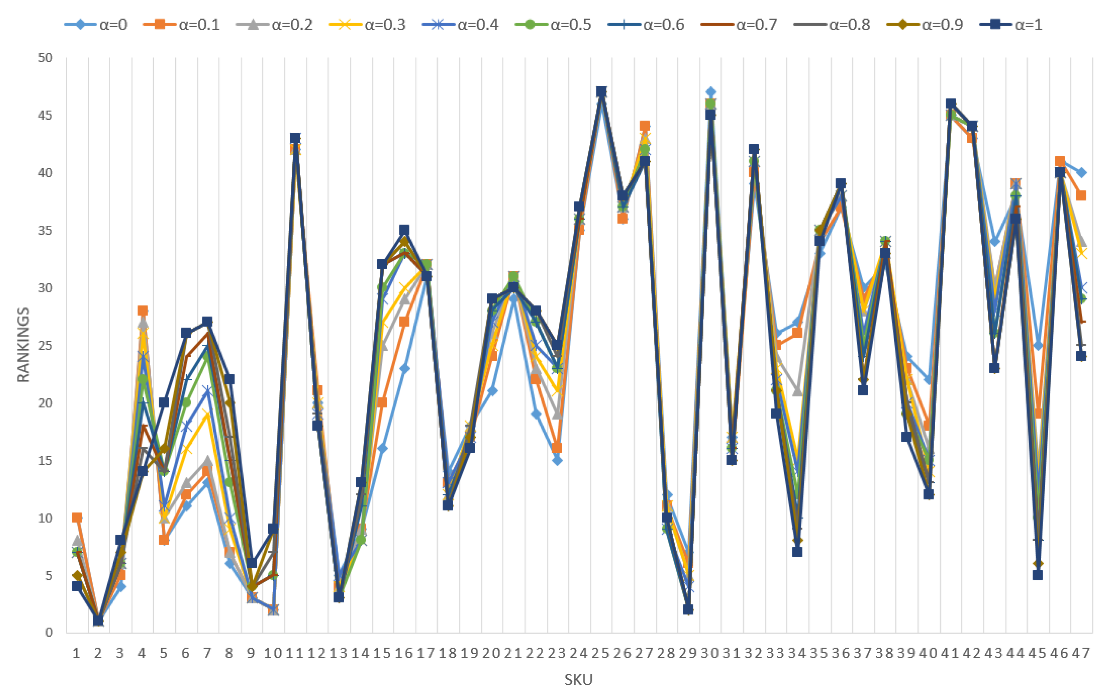
By means of incorporating the “coefficient of optimism”, , the pessimistic and optimistic outcomes are thereby balanced to mitigate the uncertainty in decision making. We ranked all SKUs based on different values of and report them in Table 3 and Figure 1.
- as increases from zero to one, the changes of the rankings are almost monotonic, indicating that the attitudes of decision makers on the risk will have a fairly significant impact on the control policy over SKUs;
- the SKUs ranking in the middle (e.g., SKU 37) have higher variability in ranking than those ranked in a high place (e.g., SKU 2) or low place (e.g., SKU 30), which means that the most and least important SKUs are easy to classify while the remaining ones are hard;
- SKU 9 ranks lower than SKU 10 when , but ranks higher when , which is in accordance with Theorem 1;
- none of the criteria determine the rankings, indicating that our methodology fully considers the preferences among these criteria.
In line with previous literature on multicriteria ABC inventory classification, this study maintained the same distribution of Groups A, B, and C, that is 10 in Group A, 14 in Group B, and 23 in Group C. The classification results under different values of are presented in Table 4. It is observed that:
- Twenty-eight out of 47 SKUs were classified in a robust manner;
- SKUs 1, 2, 3, 9, 13, and 29 were always categorized as Group A; SKUs 12, 19, 31, 39, and 40 remained in Group B; and SKUs 11, 16, 17, 21, 24, 25, 26, 27, 30, 32, 35, 36, 38, 41, 42, 44, and 46 were always classified into Group C;
- the classification results of remaining 19 SKUs were heavily dependent on the variation of , e.g., when and , SKU 34 was classified into Group C and Group A, respectively;
- most of the SKUs that were ranked higher (lower) as increased were observed with a relative high (low) value in LT, which indicated that individuals may prefer LT most in the optimistic situation;
- the above phenomenon also worked for AUC, but the relation was less apparent.
In terms of implementing the CRITIC method, we summarize the optimal weights associated with each individual judgments according to Equation (9). The results are shown in Table 5, in which the rankings of all individual judgments are reported in the brackets. The results revealed five preferences among these individual judgments. They were,
- , when ;
- , when ;
- , when ;
- , when ;
- , when .
We found that although we considered all possible individual judgments about the criteria’s importance order, the weight of each individual judgment still varied. The reason could be that some criteria naturally cannot discriminate SKUs. For example, the standard deviation of attribute AUC was the smallest, and CUT and CTU were always regarded as the two least important judgments.
To further demonstrate the effectiveness of the proposed method, we compare our classification results (as shown in Table 4) with the results derived from two related studies in Table 6. Note that the items in Table 6 are listed in descending order according to their rankings in the last column of Table 3.
The Ng model denotes the method proposed by Ng [18] who only considered the optimistic situation and one individual judgment UCT. It can be viewed as a special case of our method when both the coefficient and the weight are set to one. Compared with our results in optimistic situation, there were 11 of 47 SKUs that was classified differently. This was due to the fact that the Ng model ranks the criteria as ; thus, the classification results mostly depended on the scores of ADU. For example, SKU 45 with low ADU and high LT was grouped into Class B using the Ng model, but grouped into Class A using the proposed method because it also considered the situation when LT was preferred more than ADU.
The HV model [19] extends the Ng model by specifying weights for each criteria conditioned on that the ranking of the criteria has been determined. Under the same ranking as the Ng model (UCT), the classification results using the HV model are illustrated in Table 6. The results were almost in accordance with the Ng model in that if the Ng model classified one SKU in a higher (lower) group than the proposed method, then the HV model also classified it in a higher (lower) group. Therefore, our method provided a more reasonable index for multicriteria inventory classification as compared to the Ng model and HV model, since it incorporated various individual judgments about the importance order of criteria. Although one can specify different judgments manually before applying the Ng model and HV model so as to generate different results of classification, our method still was advanced in aggregating them together into a comprehensive result.
The last column of Table 6 illustrates the results derived from Fu et al. [10] who also considered that different decision makers may prefer different criteria and are unlikely to achieve a consensus. Similar to our paper, they first derived the score for each SKU with each criteria ranking and then calculated common weights associated with all rankings using a distance based decision making approach. However, they only considered the optimistic situation; thus, as is shown in Table 6, their results were quite close to our method when . That is, only four out of the 47 SKUs were classified differently. As decreased from one to zero, there were more differences. Especially when , 15 SKUs did not have the same classification. In this view, our method was more flexible by incorporating the “coefficient of optimism”.
To evaluate the robustness of our method, we conducted another experiment on 10 datasets, each of which contained 10 SKUs randomly selected from the original data without replacement. For each datum, we calculated the rankings of the SKUs and compared them with the rankings in Table 3. Since the value of affected the rankings, we only considered the risk-neutral situation, that is . The same results could be obtained for other values.
The comparisons are shown in Table 7. Take Data 1 as an example, it contained SKUs 3, 14, 45, 34, 31, 6, 20, 27, 42, and 41. These SKUs ranked 6th, 8th, 10th, 12th, 16th, 20th, 28th, 42n, 44th, and 45th out of 47 SKUs, but ranked 2nd, 1st, 3rd, 5th, 4th, 6th, 7th, 8th, 9th, and 10th in Data 1. According to the results in Table 7, we found that the order of the rankings on the third row was almost in accordance with the second row. That is, if one SKU was considered to be more important than another one in the original data, then such a relation probably held in the new data. Furthermore, the SKUs that ranked high (low) among the 47 SKUs would also be considered as important (unimportant) among the 10 SKUs. There were a few counter examples (indicated by boldface in Table 7). However, the rankings of these SKUs were close to each other in the original data, which meant that it was naturally difficult to rank them. In this sense, we concluded that our method was able to provide robust classification.
Through the above numerical experiments, we were able to conclude that our results, which took into account all possible individual judgments, were robust and effective. The methodology presented in this paper provided a new framework in dealing with the multicriteria ABC inventory classification problem. In addition, our results were originated from the simultaneous consideration of the pessimistic and optimistic results under certain individual judgment, which were then balanced by a coefficient of optimism to alleviate the uncertainty between the pessimistic and optimistic outcomes. The social choice result was then obtained by means of aggregating the individual judgments through the CRITIC method. In this sense, various ABC inventory classification results were derived with different coefficients of optimism, showing the flexibility of our methodology.
6. Conclusions
A sustainable supply chain demands the consideration of not only the economic, but also the social and environmental aspects, which cannot be achieved without efficient inventory management [33]. The ABC inventory classification is one of the fundamental problems in inventory management. It provides organizations with more efficient means for reducing emissions emanating from inventory (e.g., waste of storage and materials) and warehousing (e.g., heating, cooling, air conditioning, and lighting) with little effect on their profitability.
Almost all of the existing multicriteria ABC inventory classification literature is performed following the weighting and aggregating rationale. Very few of these works have uncovered this issue considering the various individual judgments on criteria, according to which the pessimistic (or worst, least favorable) and optimistic (or best, most favorable) results are obtained. Nevertheless, the investigation on uncertainty between pessimism and optimism is ignored. The main purpose of our study was to bridge this gap by taking advantage of the Hurwicz criterion to describe the outcome from certain individual judgment. Motivated by the social choice theory, the CRITIC method was applied to aggregate a variety of individual judgments into a collective choice decision. This paper contributes to the multicriteria ABC inventory classification literature by providing more methodological options.
Although the usefulness and robustness of the proposed methodology was demonstrated through numerical study, we expect future researchers to carry out more case studies using data from other industries or under different multicriteria decision making contexts. In addition, we only considered three criteria in the experiment, which included six possible rankings of the criteria’s importance. However, the number of possible rankings increased exponentially with respect to the number of criteria, and there was great computational burden to go through all the possibilities before aggregation. A method or algorithm to prune meaningless criteria’s importance rankings so as to generate results quickly is also expected in the future.
Author Contributions
Conceptualization, F.L. and N.M.; methodology, F.L.; software, N.M.; validation, N.M.; data curation, N.M.; writing, original draft preparation, F.L.; writing, review and editing, F.L.; funding acquisition, F.L. All authors have read and agreed to the published version of the manuscript.
Funding
This research was funded by the National Natural Science Foundation of China (No. 71801124).
Conflicts of Interest
The authors declare no conflict of interest.
References
- Soysal, M.; Cimen, M.; Belbag, S.; Togrul, E. A review on sustainable inventory routing. Comput. Ind. Eng. 2019, 132, 395–411. [Google Scholar] [CrossRef]
- Fichtinger, J.; Ries, J.M.; Grosse, E.H.; Baker, P. Assessing the environmental impact of integrated inventory and warehouse management. Int. J. Prod. Econ. 2015, 170, 717–729. [Google Scholar] [CrossRef]
- Tiwari, S.; Daryanto, Y.; Wee, H.M. Sustainable inventory management with deteriorating and imperfect quality items considering carbon emission. J. Clean. Prod. 2018, 192, 281–292. [Google Scholar] [CrossRef]
- Liu, J.; Liao, X.; Zhao, W.; Yang, N. A classification approach based on the outranking model for multiple criteria ABC analysis. Omega 2016, 61, 19–34. [Google Scholar] [CrossRef]
- Flores, B.E.; Whybark, D.C. Implementing multiple criteria ABC analysis. J. Oper. Manag. 1987, 7, 79–85. [Google Scholar] [CrossRef]
- Li, Z.; Wu, X.; Liu, F.; Fu, Y.; Chen, K. Multicriteria ABC inventory classification using acceptability analysis. Int. Trans. Oper. Res. 2019, 26, 2494–2507. [Google Scholar] [CrossRef]
- Teunter, R.H.; Babai, M.Z.; Syntetos, A.A. ABC classification: service levels and inventory costs. Prod. Oper. Manag. 2010, 19, 343–352. [Google Scholar] [CrossRef]
- Chen, Y.; Li, K.W.; Kilgour, D.M.; Hipel, K.W. A case based distance model for multiple criteria ABC analysis. Comput. Oper. Res. 2008, 35, 776–796. [Google Scholar] [CrossRef]
- Ramanathan, R. ABC inventory classification with multiple-criteria using weighted linear optimization. Comput. Oper. Res. 2006, 33, 695–700. [Google Scholar] [CrossRef]
- Fu, Y.; Lai, K.K.; Miao, Y.; Leung, J.W. A distance based decision-making method to improve multiple criteria ABC inventory classification. Int. Trans. Oper. Res. 2016, 23, 969–978. [Google Scholar] [CrossRef] [Green Version]
- Sen, A. Social choice theory: A re-examination. Econometrica 1977, 45, 53–88. [Google Scholar] [CrossRef]
- Sen, A. The possibility of social choice. Am. Econ. Rev. 1999, 89, 349–378. [Google Scholar] [CrossRef]
- Dyer, J.S.; Miles, R.F., Jr. An actual application of collective choice theory to the selection of trajectories for the Mariner Jupiter/Saturn 1977 project. Oper. Res. 1976, 24, 220–244. [Google Scholar] [CrossRef]
- Srdjevic, B. Linking analytic hierarchy process and social choice methods to support group decision-making in water management. Decis. Support Syst. 2007, 42, 2261–2273. [Google Scholar] [CrossRef]
- Diakoulaki, D.; Mavrotas, G.; Papayannakis, L. Determining objective weights in multiple criteria problems: The CRITIC method. Comput. Oper. Res. 1995, 22, 763–770. [Google Scholar] [CrossRef]
- Rostamzadeh, R.; Ghorabaee, M.K.; Govindan, K.; Esmaeili, A.; Nobar, H.B.K. Evaluation of sustainable supply chain risk management using an integrated fuzzy TOPSIS-CRITIC approach. J. Clean. Prod. 2018, 175, 651–669. [Google Scholar] [CrossRef]
- Zhou, P.; Fan, L. A note on multi-criteria ABC inventory classification using weighted linear optimization. Eur. J. Oper. Res. 2007, 182, 1488–1491. [Google Scholar] [CrossRef]
- Ng, W.L. A simple classifier for multiple criteria ABC analysis. Eur. J. Oper. Res. 2007, 177, 344–353. [Google Scholar] [CrossRef]
- Hadi-Vencheh, A. An improvement to multiple criteria ABC inventory classification. Eur. J. Oper. Res. 2010, 201, 962–965. [Google Scholar] [CrossRef]
- Tsai, C.Y.; Yeh, S.W. A multiple objective particle swarm optimization approach for inventory classification. Int. J. Prod. Econ. 2008, 114, 656–666. [Google Scholar] [CrossRef]
- Millstein, M.A.; Yang, L.; Li, H. Optimizing ABC inventory grouping decisions. Int. J. Prod. Econ. 2014, 148, 71–80. [Google Scholar] [CrossRef]
- Yang, L.; Li, H.; Campbell, J.F.; Sweeney, D.C. Integrated multi-period dynamic inventory classification and control. Int. J. Prod. Econ. 2017, 189, 86–96. [Google Scholar] [CrossRef]
- Park, J.; Bae, H.; Bae, J. Cross-evaluation based weighted linear optimization for multi-criteria ABC inventory classification. Comput. Ind. Eng. 2014, 76, 40–48. [Google Scholar] [CrossRef]
- Soylu, B.; Akyol, B. Multi-criteria inventory classification with reference items. Comput. Ind. Eng. 2014, 69, 12–20. [Google Scholar] [CrossRef]
- Iqbal, Q.; Malzahn, D. Evaluating discriminating power of single-criteria and multi-criteria models towards inventory classification. Comput. Ind. Eng. 2017, 104, 219–223. [Google Scholar] [CrossRef]
- Bhattacharya, A.; Sarkar, B.; Mukherjee, S.K. Distance based consensus method for ABC analysis. Int. J. Prod. Res. 2007, 45, 3405–3420. [Google Scholar] [CrossRef]
- Kartal, H.; Oztekin, A.; Gunasekaran, A.; Cebi, F. An integrated decision analytic framework of machine learning with multi-criteria decision making for multi-attribute inventory classification. Comput. Ind. Eng. 2016, 101, 599–613. [Google Scholar] [CrossRef]
- Ishizaka, A.; Gordon, M. MACBETHSort: a multiple criteria decision aid procedure for sorting strategic products. J. Oper. Res. Soc. 2017, 68, 53–61. [Google Scholar] [CrossRef]
- Ishizaka, A.; Lolli, F.; Balugani, E.; Cavallieri, R.; Gamberini, R. DEASort: Assigning items with data envelopment analysis in ABC classes. Int. J. Prod. Econ. 2018, 199, 7–15. [Google Scholar] [CrossRef] [Green Version]
- Melkonyan, T.; Safra, Z. Intrinsic variability in group and individual decision making. Manag. Sci. 2016, 62, 2651–2667. [Google Scholar] [CrossRef] [Green Version]
- Lahdelma, R.; Salminen, P. SMAA-2: Stochastic multicriteria acceptability analysis for group decision making. Oper. Res. 2001, 49, 444–454. [Google Scholar] [CrossRef]
- Liu, W.; Wang, Y.M. Ranking DMUs by using the upper and lower bounds of the normalized efficiency in data envelopment analysis. Comput. Ind. Eng. 2018, 125, 135–143. [Google Scholar] [CrossRef]
- Pourhejazy, P.; Kwon, O.K. The new generation of operations research methods in supply chain optimization: A review. Sustainability 2016, 8, 1033. [Google Scholar] [CrossRef] [Green Version]
Figure 1.
Comparison of rankings.


Table 1.
Data for ABC inventory classification. ADU, annual dollar usage; LT, lead time.
| SKU | ADU | AUC | LT | Normalized ADU | Normalized AUC | Normalized LT |
|---|---|---|---|---|---|---|
| 1 | 5840.64 | 49.92 | 2 | 1.0000 | 0.2187 | 0.1667 |
| 2 | 5670 | 210 | 5 | 0.9707 | 1.0000 | 0.6667 |
| 3 | 5037.12 | 23.76 | 4 | 0.8618 | 0.0910 | 0.5000 |
| 4 | 4769.56 | 27.73 | 1 | 0.8158 | 0.1104 | 0.0000 |
| 5 | 3478.8 | 57.98 | 3 | 0.5939 | 0.2580 | 0.3333 |
| 6 | 2936.67 | 31.24 | 3 | 0.5006 | 0.1275 | 0.3333 |
| 7 | 2820 | 28.2 | 3 | 0.4806 | 0.1127 | 0.3333 |
| 8 | 2640 | 55 | 4 | 0.4496 | 0.2435 | 0.5000 |
| 9 | 2423.52 | 73.44 | 6 | 0.4124 | 0.3335 | 0.8333 |
| 10 | 2407.5 | 160.5 | 4 | 0.4096 | 0.7584 | 0.5000 |
| 11 | 1075.2 | 5.12 | 2 | 0.1805 | 0.0000 | 0.1667 |
| 12 | 1043.5 | 20.87 | 5 | 0.1751 | 0.0769 | 0.6667 |
| 13 | 1038 | 86.5 | 7 | 0.1741 | 0.3972 | 1.0000 |
| 14 | 883.2 | 110.4 | 5 | 0.1475 | 0.5139 | 0.6667 |
| 15 | 854.4 | 71.2 | 3 | 0.1426 | 0.3225 | 0.3333 |
| 16 | 810 | 45 | 3 | 0.1349 | 0.1947 | 0.3333 |
| 17 | 703.68 | 14.66 | 4 | 0.1166 | 0.0466 | 0.5000 |
| 18 | 594 | 49.5 | 6 | 0.0978 | 0.2166 | 0.8333 |
| 19 | 570 | 47.5 | 5 | 0.0937 | 0.2069 | 0.6667 |
| 20 | 467.6 | 58.45 | 4 | 0.0760 | 0.2603 | 0.5000 |
| 21 | 463.6 | 24.4 | 4 | 0.0754 | 0.0941 | 0.5000 |
| 22 | 455 | 65 | 4 | 0.0739 | 0.2923 | 0.5000 |
| 23 | 432.5 | 86.5 | 4 | 0.0700 | 0.3972 | 0.5000 |
| 24 | 398.4 | 33.2 | 3 | 0.0641 | 0.1371 | 0.3333 |
| 25 | 370.5 | 37.05 | 1 | 0.0593 | 0.1558 | 0.0000 |
| 26 | 338.4 | 33.84 | 3 | 0.0538 | 0.1402 | 0.3333 |
| 27 | 336.12 | 84.03 | 1 | 0.0534 | 0.3852 | 0.0000 |
| 28 | 313.6 | 78.4 | 6 | 0.0496 | 0.3577 | 0.8333 |
| 29 | 268.68 | 134.34 | 7 | 0.0418 | 0.6307 | 1.0000 |
| 30 | 224 | 56 | 1 | 0.0342 | 0.2483 | 0.0000 |
| 31 | 216 | 72 | 5 | 0.0328 | 0.3264 | 0.6667 |
| 32 | 212.08 | 53.02 | 2 | 0.0321 | 0.2338 | 0.1667 |
| 33 | 197.92 | 49.48 | 5 | 0.0297 | 0.2165 | 0.6667 |
| 34 | 190.89 | 7.07 | 7 | 0.0285 | 0.0095 | 1.0000 |
| 35 | 181.8 | 60.6 | 3 | 0.0269 | 0.2708 | 0.3333 |
| 36 | 163.28 | 40.82 | 3 | 0.0237 | 0.1742 | 0.3333 |
| 37 | 150 | 30 | 5 | 0.0214 | 0.1214 | 0.6667 |
| 38 | 134.8 | 67.4 | 3 | 0.0188 | 0.3040 | 0.3333 |
| 39 | 119.2 | 59.6 | 5 | 0.0161 | 0.2659 | 0.6667 |
| 40 | 103.36 | 51.68 | 6 | 0.0134 | 0.2273 | 0.8333 |
| 41 | 79.2 | 19.8 | 2 | 0.0093 | 0.0717 | 0.1667 |
| 42 | 75.4 | 37.7 | 2 | 0.0086 | 0.1590 | 0.1667 |
| 43 | 59.78 | 29.89 | 5 | 0.0059 | 0.1209 | 0.6667 |
| 44 | 48.3 | 48.3 | 3 | 0.0039 | 0.2108 | 0.3333 |
| 45 | 34.4 | 34.4 | 7 | 0.0016 | 0.1429 | 1.0000 |
| 46 | 28.8 | 28.8 | 3 | 0.0006 | 0.1156 | 0.3333 |
| 47 | 25.38 | 8.46 | 5 | 0.0000 | 0.0163 | 0.6667 |
Table 2.
The pessimistic and optimistic results.
| SKU | Pessimistic Results | Optimistic Results | ||||||||||
|---|---|---|---|---|---|---|---|---|---|---|---|---|
| CUT | CTU | UCT | UTC | TCU | TUC | CUT | CTU | UCT | UTC | TCU | TUC | |
| 1 | 0.2187 | 0.1927 | 0.4618 | 0.4618 | 0.1667 | 0.1667 | 0.6093 | 0.4618 | 1.0000 | 1.0000 | 0.4618 | 0.5833 |
| 2 | 0.8791 | 0.8333 | 0.8791 | 0.8187 | 0.6667 | 0.6667 | 1.0000 | 1.0000 | 0.9853 | 0.9707 | 0.8791 | 0.8791 |
| 3 | 0.0910 | 0.0910 | 0.4764 | 0.4843 | 0.2955 | 0.4843 | 0.4843 | 0.4843 | 0.8618 | 0.8618 | 0.5000 | 0.6809 |
| 4 | 0.1104 | 0.0552 | 0.3087 | 0.3087 | 0.0000 | 0.0000 | 0.4631 | 0.3087 | 0.8158 | 0.8158 | 0.3087 | 0.4079 |
| 5 | 0.2580 | 0.2580 | 0.3951 | 0.3951 | 0.2957 | 0.3333 | 0.4259 | 0.3951 | 0.5939 | 0.5939 | 0.3951 | 0.4636 |
| 6 | 0.1275 | 0.1275 | 0.3141 | 0.3205 | 0.2304 | 0.3205 | 0.3205 | 0.3205 | 0.5006 | 0.5006 | 0.3333 | 0.4170 |
| 7 | 0.1127 | 0.1127 | 0.2966 | 0.3089 | 0.2230 | 0.3089 | 0.3089 | 0.3089 | 0.4806 | 0.4806 | 0.3333 | 0.4069 |
| 8 | 0.2435 | 0.2435 | 0.3465 | 0.3977 | 0.3717 | 0.3977 | 0.3977 | 0.3977 | 0.4496 | 0.4748 | 0.5000 | 0.5000 |
| 9 | 0.3335 | 0.3335 | 0.3729 | 0.4124 | 0.5264 | 0.5264 | 0.5264 | 0.5834 | 0.5264 | 0.6229 | 0.8333 | 0.8333 |
| 10 | 0.5560 | 0.5560 | 0.4096 | 0.4096 | 0.5000 | 0.4548 | 0.7584 | 0.7584 | 0.5840 | 0.5560 | 0.6292 | 0.5560 |
| 11 | 0.0000 | 0.0000 | 0.0903 | 0.1157 | 0.0833 | 0.1157 | 0.1157 | 0.1157 | 0.1805 | 0.1805 | 0.1667 | 0.1736 |
| 12 | 0.0769 | 0.0769 | 0.1260 | 0.1751 | 0.3062 | 0.3062 | 0.3062 | 0.3718 | 0.3062 | 0.4209 | 0.6667 | 0.6667 |
| 13 | 0.2857 | 0.3972 | 0.1741 | 0.1741 | 0.5238 | 0.5238 | 0.5238 | 0.6986 | 0.5238 | 0.5871 | 1.0000 | 1.0000 |
| 14 | 0.3307 | 0.4427 | 0.1475 | 0.1475 | 0.4427 | 0.4071 | 0.5139 | 0.5903 | 0.4427 | 0.4427 | 0.6667 | 0.6667 |
| 15 | 0.2325 | 0.2661 | 0.1426 | 0.1426 | 0.2661 | 0.2379 | 0.3225 | 0.3279 | 0.2661 | 0.2661 | 0.3333 | 0.3333 |
| 16 | 0.1648 | 0.1947 | 0.1349 | 0.1349 | 0.2210 | 0.2210 | 0.2210 | 0.2640 | 0.2210 | 0.2341 | 0.3333 | 0.3333 |
| 17 | 0.0466 | 0.0466 | 0.0816 | 0.1166 | 0.2211 | 0.2211 | 0.2211 | 0.2733 | 0.2211 | 0.3083 | 0.5000 | 0.5000 |
| 18 | 0.1572 | 0.2166 | 0.0978 | 0.0978 | 0.3826 | 0.3826 | 0.3826 | 0.5250 | 0.3826 | 0.4656 | 0.8333 | 0.8333 |
| 19 | 0.1503 | 0.2069 | 0.0937 | 0.0937 | 0.3224 | 0.3224 | 0.3224 | 0.4368 | 0.3224 | 0.3802 | 0.6667 | 0.6667 |
| 20 | 0.1682 | 0.2603 | 0.0760 | 0.0760 | 0.2788 | 0.2788 | 0.2788 | 0.3801 | 0.2788 | 0.2880 | 0.5000 | 0.5000 |
| 21 | 0.0847 | 0.0941 | 0.0754 | 0.0754 | 0.2232 | 0.2232 | 0.2232 | 0.2971 | 0.2232 | 0.2877 | 0.5000 | 0.5000 |
| 22 | 0.1831 | 0.2887 | 0.0739 | 0.0739 | 0.2887 | 0.2869 | 0.2923 | 0.3961 | 0.2887 | 0.2887 | 0.5000 | 0.5000 |
| 23 | 0.2336 | 0.3224 | 0.0700 | 0.0700 | 0.3224 | 0.2850 | 0.3972 | 0.4486 | 0.3224 | 0.3224 | 0.5000 | 0.5000 |
| 24 | 0.1006 | 0.1371 | 0.0641 | 0.0641 | 0.1782 | 0.1782 | 0.1782 | 0.2352 | 0.1782 | 0.1987 | 0.3333 | 0.3333 |
| 25 | 0.0717 | 0.0717 | 0.0593 | 0.0297 | 0.0000 | 0.0000 | 0.1558 | 0.1558 | 0.1076 | 0.0717 | 0.0779 | 0.0717 |
| 26 | 0.0970 | 0.1402 | 0.0538 | 0.0538 | 0.1758 | 0.1758 | 0.1758 | 0.2368 | 0.1758 | 0.1936 | 0.3333 | 0.3333 |
| 27 | 0.1462 | 0.1462 | 0.0534 | 0.0267 | 0.0000 | 0.0000 | 0.3852 | 0.3852 | 0.2193 | 0.1462 | 0.1926 | 0.1462 |
| 28 | 0.2036 | 0.3577 | 0.0496 | 0.0496 | 0.4135 | 0.4135 | 0.4135 | 0.5955 | 0.4135 | 0.4414 | 0.8333 | 0.8333 |
| 29 | 0.3363 | 0.5575 | 0.0418 | 0.0418 | 0.5575 | 0.5209 | 0.6307 | 0.8154 | 0.5575 | 0.5575 | 1.0000 | 1.0000 |
| 30 | 0.0942 | 0.0942 | 0.0342 | 0.0171 | 0.0000 | 0.0000 | 0.2483 | 0.2483 | 0.1412 | 0.0942 | 0.1242 | 0.0942 |
| 31 | 0.1796 | 0.3264 | 0.0328 | 0.0328 | 0.3420 | 0.3420 | 0.3420 | 0.4966 | 0.3420 | 0.3497 | 0.6667 | 0.6667 |
| 32 | 0.1330 | 0.1442 | 0.0321 | 0.0321 | 0.1442 | 0.0994 | 0.2338 | 0.2338 | 0.1442 | 0.1442 | 0.2002 | 0.1667 |
| 33 | 0.1231 | 0.2165 | 0.0297 | 0.0297 | 0.3043 | 0.3043 | 0.3043 | 0.4416 | 0.3043 | 0.3482 | 0.6667 | 0.6667 |
| 34 | 0.0095 | 0.0095 | 0.0190 | 0.0285 | 0.3460 | 0.3460 | 0.3460 | 0.5048 | 0.3460 | 0.5142 | 1.0000 | 1.0000 |
| 35 | 0.1488 | 0.2103 | 0.0269 | 0.0269 | 0.2103 | 0.1801 | 0.2708 | 0.3021 | 0.2103 | 0.2103 | 0.3333 | 0.3333 |
| 36 | 0.0990 | 0.1742 | 0.0237 | 0.0237 | 0.1771 | 0.1771 | 0.1771 | 0.2538 | 0.1771 | 0.1785 | 0.3333 | 0.3333 |
| 37 | 0.0714 | 0.1214 | 0.0214 | 0.0214 | 0.2698 | 0.2698 | 0.2698 | 0.3941 | 0.2698 | 0.3440 | 0.6667 | 0.6667 |
| 38 | 0.1614 | 0.2187 | 0.0188 | 0.0188 | 0.2187 | 0.1761 | 0.3040 | 0.3187 | 0.2187 | 0.2187 | 0.3333 | 0.3333 |
| 39 | 0.1410 | 0.2659 | 0.0161 | 0.0161 | 0.3162 | 0.3162 | 0.3162 | 0.4663 | 0.3162 | 0.3414 | 0.6667 | 0.6667 |
| 40 | 0.1203 | 0.2273 | 0.0134 | 0.0134 | 0.3580 | 0.3580 | 0.3580 | 0.5303 | 0.3580 | 0.4234 | 0.8333 | 0.8333 |
| 41 | 0.0405 | 0.0717 | 0.0093 | 0.0093 | 0.0825 | 0.0825 | 0.0825 | 0.1192 | 0.0825 | 0.0880 | 0.1667 | 0.1667 |
| 42 | 0.0838 | 0.1114 | 0.0086 | 0.0086 | 0.1114 | 0.0876 | 0.1590 | 0.1628 | 0.1114 | 0.1114 | 0.1667 | 0.1667 |
| 43 | 0.0634 | 0.1209 | 0.0059 | 0.0059 | 0.2645 | 0.2645 | 0.2645 | 0.3938 | 0.2645 | 0.3363 | 0.6667 | 0.6667 |
| 44 | 0.1073 | 0.1827 | 0.0039 | 0.0039 | 0.1827 | 0.1686 | 0.2108 | 0.2720 | 0.1827 | 0.1827 | 0.3333 | 0.3333 |
| 45 | 0.0722 | 0.1429 | 0.0016 | 0.0016 | 0.3815 | 0.3815 | 0.3815 | 0.5715 | 0.3815 | 0.5008 | 1.0000 | 1.0000 |
| 46 | 0.0581 | 0.1156 | 0.0006 | 0.0006 | 0.1498 | 0.1498 | 0.1498 | 0.2245 | 0.1498 | 0.1670 | 0.3333 | 0.3333 |
| 47 | 0.0082 | 0.0163 | 0.0000 | 0.0000 | 0.2277 | 0.2277 | 0.2277 | 0.3415 | 0.2277 | 0.3333 | 0.6667 | 0.6667 |
Table 3.
Rankings under the Hurwicz criterion.
| SKU | ADU | AUC | LT | |||||||||||
|---|---|---|---|---|---|---|---|---|---|---|---|---|---|---|
| 1 | 5840.64 | 49.92 | 2 | 10 | 10 | 8 | 7 | 7 | 7 | 7 | 7 | 5 | 5 | 4 |
| 2 | 5670 | 210 | 5 | 1 | 1 | 1 | 1 | 1 | 1 | 1 | 1 | 1 | 1 | 1 |
| 3 | 5037.12 | 23.76 | 4 | 4 | 5 | 6 | 6 | 6 | 6 | 6 | 6 | 6 | 7 | 8 |
| 4 | 4769.56 | 27.73 | 1 | 28 | 28 | 27 | 26 | 24 | 22 | 20 | 18 | 16 | 14 | 14 |
| 5 | 3478.8 | 57.98 | 3 | 8 | 8 | 10 | 10 | 11 | 14 | 14 | 14 | 14 | 16 | 20 |
| 6 | 2936.67 | 31.24 | 3 | 11 | 12 | 13 | 16 | 18 | 20 | 22 | 24 | 26 | 26 | 26 |
| 7 | 2820 | 28.2 | 3 | 13 | 14 | 15 | 19 | 21 | 24 | 25 | 26 | 27 | 27 | 27 |
| 8 | 2640 | 55 | 4 | 6 | 7 | 7 | 9 | 10 | 13 | 15 | 15 | 17 | 20 | 22 |
| 9 | 2423.52 | 73.44 | 6 | 3 | 3 | 3 | 3 | 3 | 4 | 4 | 4 | 4 | 4 | 6 |
| 10 | 2407.5 | 160.5 | 4 | 2 | 2 | 2 | 2 | 2 | 5 | 5 | 5 | 7 | 9 | 9 |
| 11 | 1075.2 | 5.12 | 2 | 42 | 42 | 42 | 42 | 43 | 43 | 43 | 43 | 43 | 43 | 43 |
| 12 | 1043.5 | 20.87 | 5 | 20 | 21 | 20 | 20 | 19 | 18 | 18 | 19 | 19 | 18 | 18 |
| 13 | 1038 | 86.5 | 7 | 5 | 4 | 4 | 4 | 5 | 3 | 3 | 3 | 3 | 3 | 3 |
| 14 | 883.2 | 110.4 | 5 | 9 | 9 | 9 | 8 | 8 | 8 | 11 | 12 | 12 | 13 | 13 |
| 15 | 854.4 | 71.2 | 3 | 16 | 20 | 25 | 27 | 29 | 30 | 32 | 32 | 32 | 32 | 32 |
| 16 | 810 | 45 | 3 | 23 | 27 | 29 | 30 | 33 | 33 | 33 | 33 | 34 | 34 | 35 |
| 17 | 703.68 | 14.66 | 4 | 31 | 32 | 32 | 32 | 32 | 32 | 31 | 31 | 31 | 31 | 31 |
| 18 | 594 | 49.5 | 6 | 14 | 13 | 12 | 12 | 13 | 11 | 12 | 11 | 11 | 11 | 11 |
| 19 | 570 | 47.5 | 5 | 18 | 17 | 18 | 18 | 17 | 17 | 17 | 17 | 18 | 17 | 16 |
| 20 | 467.6 | 58.45 | 4 | 21 | 24 | 26 | 25 | 27 | 28 | 28 | 29 | 29 | 29 | 29 |
| 21 | 463.6 | 24.4 | 4 | 29 | 31 | 31 | 31 | 31 | 31 | 30 | 30 | 30 | 30 | 30 |
| 22 | 455 | 65 | 4 | 19 | 22 | 23 | 24 | 25 | 27 | 27 | 28 | 28 | 28 | 28 |
| 23 | 432.5 | 86.5 | 4 | 15 | 16 | 19 | 21 | 23 | 23 | 23 | 25 | 24 | 25 | 25 |
| 24 | 398.4 | 33.2 | 3 | 35 | 35 | 36 | 36 | 36 | 36 | 36 | 36 | 37 | 37 | 37 |
| 25 | 370.5 | 37.05 | 1 | 46 | 47 | 47 | 47 | 47 | 47 | 47 | 47 | 47 | 47 | 47 |
| 26 | 338.4 | 33.84 | 3 | 36 | 36 | 37 | 37 | 37 | 37 | 37 | 38 | 38 | 38 | 38 |
| 27 | 336.12 | 84.03 | 1 | 44 | 44 | 43 | 43 | 42 | 42 | 41 | 41 | 41 | 41 | 41 |
| 28 | 313.6 | 78.4 | 6 | 12 | 11 | 11 | 11 | 9 | 9 | 9 | 10 | 10 | 10 | 10 |
| 29 | 268.68 | 134.34 | 7 | 7 | 6 | 5 | 5 | 4 | 2 | 2 | 2 | 2 | 2 | 2 |
| 30 | 224 | 56 | 1 | 47 | 46 | 46 | 46 | 46 | 46 | 45 | 45 | 45 | 45 | 45 |
| 31 | 216 | 72 | 5 | 17 | 15 | 17 | 17 | 16 | 16 | 16 | 16 | 15 | 15 | 15 |
| 32 | 212.08 | 53.02 | 2 | 39 | 40 | 41 | 41 | 41 | 41 | 42 | 42 | 42 | 42 | 42 |
| 33 | 197.92 | 49.48 | 5 | 26 | 25 | 24 | 23 | 22 | 21 | 21 | 21 | 21 | 21 | 19 |
| 34 | 190.89 | 7.07 | 7 | 27 | 26 | 21 | 15 | 14 | 12 | 10 | 9 | 9 | 8 | 7 |
| 35 | 181.8 | 60.6 | 3 | 33 | 34 | 35 | 35 | 35 | 35 | 35 | 35 | 35 | 35 | 34 |
| 36 | 163.28 | 40.82 | 3 | 37 | 37 | 38 | 38 | 38 | 39 | 39 | 39 | 39 | 39 | 39 |
| 37 | 150 | 30 | 5 | 30 | 29 | 28 | 28 | 26 | 25 | 24 | 22 | 22 | 22 | 21 |
| 38 | 134.8 | 67.4 | 3 | 32 | 33 | 33 | 34 | 34 | 34 | 34 | 34 | 33 | 33 | 33 |
| 39 | 119.2 | 59.6 | 5 | 24 | 23 | 22 | 22 | 20 | 19 | 19 | 20 | 20 | 19 | 17 |
| 40 | 103.36 | 51.68 | 6 | 22 | 18 | 16 | 14 | 15 | 15 | 13 | 13 | 13 | 12 | 12 |
| 41 | 79.2 | 19.8 | 2 | 45 | 45 | 45 | 45 | 45 | 45 | 46 | 46 | 46 | 46 | 46 |
| 42 | 75.4 | 37.7 | 2 | 43 | 43 | 44 | 44 | 44 | 44 | 44 | 44 | 44 | 44 | 44 |
| 43 | 59.78 | 29.89 | 5 | 34 | 30 | 30 | 29 | 28 | 26 | 26 | 23 | 23 | 23 | 23 |
| 44 | 48.3 | 48.3 | 3 | 38 | 39 | 39 | 39 | 39 | 38 | 38 | 37 | 36 | 36 | 36 |
| 45 | 34.4 | 34.4 | 7 | 25 | 19 | 14 | 13 | 12 | 10 | 8 | 8 | 8 | 6 | 5 |
| 46 | 28.8 | 28.8 | 3 | 41 | 41 | 40 | 40 | 40 | 40 | 40 | 40 | 40 | 40 | 40 |
| 47 | 25.38 | 8.46 | 5 | 40 | 38 | 34 | 33 | 30 | 29 | 29 | 27 | 25 | 24 | 24 |
Table 4.
ABC inventory classification results under the Hurwicz criterion.
| SKU | ADU | AUC | LT | |||||||||||
|---|---|---|---|---|---|---|---|---|---|---|---|---|---|---|
| 1 | 5840.64 | 49.92 | 2 | A | A | A | A | A | A | A | A | A | A | A |
| 2 | 5670 | 210 | 5 | A | A | A | A | A | A | A | A | A | A | A |
| 3 | 5037.12 | 23.76 | 4 | A | A | A | A | A | A | A | A | A | A | A |
| 4 | 4769.56 | 27.73 | 1 | C | C | C | C | B | B | B | B | B | B | B |
| 5 | 3478.8 | 57.98 | 3 | A | A | A | A | B | B | B | B | B | B | B |
| 6 | 2936.67 | 31.24 | 3 | B | B | B | B | B | B | B | B | C | C | C |
| 7 | 2820 | 28.2 | 3 | B | B | B | B | B | B | C | C | C | C | C |
| 8 | 2640 | 55 | 4 | A | A | A | A | A | B | B | B | B | B | B |
| 9 | 2423.52 | 73.44 | 6 | A | A | A | A | A | A | A | A | A | A | A |
| 10 | 2407.5 | 160.5 | 4 | A | A | A | A | A | A | A | A | A | A | A |
| 11 | 1075.2 | 5.12 | 2 | C | C | C | C | C | C | C | C | C | C | C |
| 12 | 1043.5 | 20.87 | 5 | B | B | B | B | B | B | B | B | B | B | B |
| 13 | 1038 | 86.5 | 7 | A | A | A | A | A | A | A | A | A | A | A |
| 14 | 883.2 | 110.4 | 5 | A | A | A | A | A | A | B | B | B | B | B |
| 15 | 854.4 | 71.2 | 3 | B | B | C | C | C | C | C | C | C | C | C |
| 16 | 810 | 45 | 3 | B | C | C | C | C | C | C | C | C | C | C |
| 17 | 703.68 | 14.66 | 4 | C | C | C | C | C | C | C | C | C | C | C |
| 18 | 594 | 49.5 | 6 | B | B | B | B | B | B | B | B | B | B | B |
| 19 | 570 | 47.5 | 5 | B | B | B | B | B | B | B | B | B | B | B |
| 20 | 467.6 | 58.45 | 4 | B | B | C | C | C | C | C | C | C | C | C |
| 21 | 463.6 | 24.4 | 4 | C | C | C | C | C | C | C | C | C | C | C |
| 22 | 455 | 65 | 4 | B | B | B | B | C | C | C | C | C | C | C |
| 23 | 432.5 | 86.5 | 4 | B | B | B | B | B | B | B | C | B | C | C |
| 24 | 398.4 | 33.2 | 3 | C | C | C | C | C | C | C | C | C | C | C |
| 25 | 370.5 | 37.05 | 1 | C | C | C | C | C | C | C | C | C | C | C |
| 26 | 338.4 | 33.84 | 3 | C | C | C | C | C | C | C | C | C | C | C |
| 27 | 336.12 | 84.03 | 1 | C | C | C | C | C | C | C | C | C | C | C |
| 28 | 313.6 | 78.4 | 6 | B | B | B | B | A | A | A | A | A | A | A |
| 29 | 268.68 | 134.34 | 7 | A | A | A | A | A | A | A | A | A | A | A |
| 30 | 224 | 56 | 1 | C | C | C | C | C | C | C | C | C | C | C |
| 31 | 216 | 72 | 5 | B | B | B | B | B | B | B | B | B | B | B |
| 32 | 212.08 | 53.02 | 2 | C | C | C | C | C | C | C | C | C | C | C |
| 33 | 197.92 | 49.48 | 5 | C | C | B | B | B | B | B | B | B | B | B |
| 34 | 190.89 | 7.07 | 7 | C | C | B | B | B | B | A | A | A | A | A |
| 35 | 181.8 | 60.6 | 3 | C | C | C | C | C | C | C | C | C | C | C |
| 36 | 163.28 | 40.82 | 3 | C | C | C | C | C | C | C | C | C | C | C |
| 37 | 150 | 30 | 5 | C | C | C | C | C | C | B | B | B | B | B |
| 38 | 134.8 | 67.4 | 3 | C | C | C | C | C | C | C | C | C | C | C |
| 39 | 119.2 | 59.6 | 5 | B | B | B | B | B | B | B | B | B | B | B |
| 40 | 103.36 | 51.68 | 6 | B | B | B | B | B | B | B | B | B | B | B |
| 41 | 79.2 | 19.8 | 2 | C | C | C | C | C | C | C | C | C | C | C |
| 42 | 75.4 | 37.7 | 2 | C | C | C | C | C | C | C | C | C | C | C |
| 43 | 59.78 | 29.89 | 5 | C | C | C | C | C | C | C | B | B | B | B |
| 44 | 48.3 | 48.3 | 3 | C | C | C | C | C | C | C | C | C | C | C |
| 45 | 34.4 | 34.4 | 7 | C | B | B | B | B | A | A | A | A | A | A |
| 46 | 28.8 | 28.8 | 3 | C | C | C | C | C | C | C | C | C | C | C |
| 47 | 25.38 | 8.46 | 5 | C | C | C | C | C | C | C | C | C | B | B |
Table 5.
Optimal weights for different preferences.
| 0.1066 [6] | 0.1466 [5] | 0.1806 [4] | 0.1967 [1] | 0.1860 [2] | 0.1835 [3] | |
| 0.1064 [6] | 0.1396 [5] | 0.1801 [4] | 0.1926 [2] | 0.1938 [1] | 0.1874 [3] | |
| 0.1067 [6] | 0.1335 [5] | 0.1790 [4] | 0.1868 [3] | 0.2020 [1] | 0.1920 [2] | |
| 0.1071 [6] | 0.1279 [5] | 0.1777 [4] | 0.1812 [3] | 0.2097 [1] | 0.1963 [2] | |
| 0.1076 [6] | 0.1228 [5] | 0.1767 [3] | 0.1759 [4] | 0.2168 [1] | 0.2002 [2] | |
| 0.1085 [6] | 0.1183 [5] | 0.1761 [3] | 0.1713 [4] | 0.2219 [1] | 0.2039 [2] | |
| 0.1100 [6] | 0.1155 [5] | 0.1776 [3] | 0.1683 [4] | 0.2235 [1] | 0.2051 [2] | |
| 0.1116 [6] | 0.1135 [5] | 0.1799 [3] | 0.1658 [4] | 0.2254 [1] | 0.2037 [2] | |
| 0.1132 [5] | 0.1119 [6] | 0.1824 [3] | 0.1635 [4] | 0.2268 [1] | 0.2022 [2] | |
| 0.1149 [5] | 0.1105 [6] | 0.1849 [3] | 0.1614 [4] | 0.2278 [1] | 0.2005 [2] | |
| 0.1175 [5] | 0.1104 [6] | 0.1860 [3] | 0.1557 [4] | 0.2301 [1] | 0.2002 [2] |
Table 6.
A comparison of our proposed method, the Ng model, the HV model, and the Fu model. All the differences of classification are indicated with bold.
Table 6.
A comparison of our proposed method, the Ng model, the HV model, and the Fu model. All the differences of classification are indicated with bold.
| SKU | ADU | AUC | LT | Proposed Method ( = 1) | Ng Model | HV Model | Fu Model |
|---|---|---|---|---|---|---|---|
| 2 | 5670 | 210 | 5 | A | A | A | A |
| 29 | 268.68 | 134.34 | 7 | A | A | A | A |
| 13 | 1038 | 86.5 | 7 | A | A | A | A |
| 1 | 5840.64 | 49.92 | 2 | A | A | A | A |
| 45 | 34.4 | 34.4 | 7 | A | B | B | A |
| 9 | 2423.52 | 73.44 | 6 | A | A | A | A |
| 34 | 190.89 | 7.07 | 7 | A | B | B | B |
| 3 | 5037.12 | 23.76 | 4 | A | A | A | A |
| 10 | 2407.5 | 160.5 | 4 | A | A | A | A |
| 28 | 313.6 | 78.4 | 6 | A | B | B | A |
| 18 | 594 | 49.5 | 6 | B | B | B | B |
| 40 | 103.36 | 51.68 | 6 | B | B | B | B |
| 14 | 883.2 | 110.4 | 5 | B | B | A | A |
| 4 | 4769.56 | 27.73 | 1 | B | A | A | B |
| 31 | 216 | 72 | 5 | B | B | B | B |
| 19 | 570 | 47.5 | 5 | B | B | B | B |
| 39 | 119.2 | 59.6 | 5 | B | B | B | B |
| 12 | 1043.5 | 20.87 | 5 | B | B | B | B |
| 33 | 197.92 | 49.48 | 5 | B | B | B | B |
| 5 | 3478.8 | 57.98 | 3 | B | A | A | B |
| 37 | 150 | 30 | 5 | B | C | C | B |
| 8 | 2640 | 55 | 4 | B | B | B | B |
| 43 | 59.78 | 29.89 | 5 | B | C | C | B |
| 47 | 25.38 | 8.46 | 5 | B | C | C | C |
| 23 | 432.5 | 86.5 | 4 | C | B | B | B |
| 6 | 2936.67 | 31.24 | 3 | C | A | B | C |
| 7 | 2820 | 28.2 | 3 | C | B | B | C |
| 22 | 455 | 65 | 4 | C | C | C | C |
| 20 | 467.6 | 58.45 | 4 | C | C | C | C |
| 21 | 463.6 | 24.4 | 4 | C | C | C | C |
| 17 | 703.68 | 14.66 | 4 | C | C | C | C |
| 15 | 854.4 | 71.2 | 3 | C | C | C | C |
| 38 | 134.8 | 67.4 | 3 | C | C | C | C |
| 35 | 181.8 | 60.6 | 3 | C | C | C | C |
| 16 | 810 | 45 | 3 | C | C | C | C |
| 44 | 48.3 | 48.3 | 3 | C | C | C | C |
| 24 | 398.4 | 33.2 | 3 | C | C | C | C |
| 26 | 338.4 | 33.84 | 3 | C | C | C | C |
| 36 | 163.28 | 40.82 | 3 | C | C | C | C |
| 46 | 28.8 | 28.8 | 3 | C | C | C | C |
| 27 | 336.12 | 84.03 | 1 | C | C | C | C |
| 32 | 212.08 | 53.02 | 2 | C | C | C | C |
| 11 | 1075.2 | 5.12 | 2 | C | C | C | C |
| 42 | 75.4 | 37.7 | 2 | C | C | C | C |
| 30 | 224 | 56 | 1 | C | C | C | C |
| 41 | 79.2 | 19.8 | 2 | C | C | C | C |
| 25 | 370.5 | 37.05 | 1 | C | C | C | C |
Table 7.
Comparisons of 10 simulation data. All counter examples are indicated by boldface.
| Data | Comparisons | ||||||||||
|---|---|---|---|---|---|---|---|---|---|---|---|
| Data 1 | SKU Number | 3 | 14 | 45 | 34 | 31 | 6 | 20 | 27 | 42 | 41 |
| Table 3 Ranking | 6 | 8 | 10 | 12 | 16 | 20 | 28 | 42 | 44 | 45 | |
| Present Ranking | 2 | 1 | 3 | 5 | 4 | 6 | 7 | 8 | 9 | 10 | |
| Data 2 | SKU Number | 29 | 10 | 45 | 8 | 40 | 22 | 20 | 15 | 17 | 36 |
| Table 3 Ranking | 2 | 5 | 10 | 13 | 15 | 27 | 28 | 30 | 32 | 39 | |
| Present Ranking | 2 | 1 | 4 | 3 | 5 | 6 | 7 | 8 | 9 | 10 | |
| Data 3 | SKU Number | 10 | 1 | 14 | 45 | 6 | 16 | 35 | 46 | 41 | 30 |
| Table 3 Ranking | 5 | 7 | 8 | 10 | 20 | 33 | 35 | 40 | 45 | 46 | |
| Present Ranking | 1 | 2 | 3 | 4 | 5 | 6 | 7 | 8 | 10 | 9 | |
| Data 4 | SKU Number | 13 | 10 | 3 | 8 | 40 | 31 | 23 | 22 | 21 | 32 |
| Table 3 Ranking | 3 | 5 | 6 | 13 | 15 | 16 | 23 | 27 | 31 | 41 | |
| Present Ranking | 2 | 1 | 3 | 4 | 5 | 6 | 7 | 8 | 9 | 10 | |
| Data 5 | SKU Number | 13 | 8 | 40 | 31 | 22 | 21 | 17 | 24 | 26 | 42 |
| Table 3 Ranking | 3 | 13 | 15 | 16 | 27 | 31 | 32 | 36 | 37 | 44 | |
| Present Ranking | 1 | 2 | 4 | 3 | 5 | 6 | 7 | 8 | 9 | 10 | |
| Data 6 | SKU Number | 2 | 45 | 18 | 5 | 40 | 7 | 35 | 26 | 36 | 27 |
| Table 3 Ranking | 1 | 10 | 11 | 14 | 15 | 24 | 35 | 37 | 39 | 42 | |
| Present Ranking | 1 | 2 | 3 | 5 | 4 | 6 | 7 | 9 | 8 | 10 | |
| Data 7 | SKU Number | 10 | 14 | 18 | 40 | 31 | 7 | 47 | 15 | 16 | 26 |
| Table 3 Ranking | 5 | 8 | 11 | 15 | 16 | 24 | 29 | 30 | 33 | 37 | |
| Present Ranking | 1 | 3 | 2 | 4 | 5 | 6 | 7 | 8 | 9 | 10 | |
| Data 8 | SKU Number | 1 | 14 | 5 | 12 | 47 | 21 | 16 | 26 | 44 | 42 |
| Table 3 Ranking | 7 | 8 | 14 | 18 | 29 | 31 | 33 | 37 | 38 | 44 | |
| Present Ranking | 2 | 1 | 3 | 4 | 5 | 6 | 7 | 9 | 8 | 10 | |
| Data 9 | SKU Number | 2 | 13 | 31 | 6 | 4 | 37 | 16 | 26 | 46 | 30 |
| Table 3 Ranking | 1 | 3 | 16 | 20 | 22 | 25 | 33 | 37 | 40 | 46 | |
| Present Ranking | 1 | 2 | 3 | 5 | 4 | 6 | 7 | 8 | 9 | 10 | |
| Data 10 | SKU Number | 3 | 28 | 18 | 6 | 23 | 22 | 20 | 16 | 46 | 11 |
| Table 3 Ranking | 6 | 9 | 11 | 20 | 23 | 27 | 28 | 33 | 40 | 43 | |
| Present Ranking | 1 | 2 | 3 | 5 | 4 | 6 | 7 | 8 | 9 | 10 | |
© 2019 by the authors. Licensee MDPI, Basel, Switzerland. This article is an open access article distributed under the terms and conditions of the Creative Commons Attribution (CC BY) license (http://creativecommons.org/licenses/by/4.0/).
Share and Cite
MDPI and ACS Style
Liu, F.; Ma, N. Multicriteria ABC Inventory Classification Using the Social Choice Theory. Sustainability 2020, 12, 182. https://doi.org/10.3390/su12010182
AMA Style
Liu F, Ma N. Multicriteria ABC Inventory Classification Using the Social Choice Theory. Sustainability. 2020; 12(1):182. https://doi.org/10.3390/su12010182
Chicago/Turabian StyleLiu, Fan, and Ning Ma. 2020. "Multicriteria ABC Inventory Classification Using the Social Choice Theory" Sustainability 12, no. 1: 182. https://doi.org/10.3390/su12010182
Note that from the first issue of 2016, this journal uses article numbers instead of page numbers. See further details here.