A Sustainability-Oriented Enhanced Indexation Model with Regime Switching and Cardinality Constraint

Abstract

Enhanced indexation is an active portfolio management strategy aimed to find a portfolio outperforming a market index. To ensure stable returns and to avoid extreme losses, a sensible enhanced indexation model should be sustainable, where the parameters of the model should be adjusted adaptively according to the market environment. Hence, in this paper, we propose a novel sustainable regime-based cardinality constrained enhanced indexation (RCEI) model, where different benchmarks and cardinalities can be imposed under different market regimes. By using historical observations, the RCEI model is transformed into a deterministic optimization problem with an ${\ell }_0$ norm constraint. We design a partial penalty method coupled with the proximal alternating direction method of multipliers (ADMM) to solve the deterministic optimization problem. Numerical results in UK and US financial markets confirm the superb performance of the sustainability-oriented RCEI model and the efficiency of the algorithm.

1. Introduction

As the global financial market is riddled with more and more uncertainty, there is a growing awareness of incorporating sustainability-relates insights into investment analysis and management; therefore, investors boost their chances for long-term and sustainable success. Incorporating sustainability insights can provide a more holistic view of the risks and opportunities associated with a given investment. In response to the increasing interest, there is a strong need to develop sustainable investing approaches and products.

The research on financial sustainability is in its infancy as only a handful of articles briefly touched on it [1,2,3,4,5,6]. Nurmakhanova et al. [3] claimed that a sustainable microfinance institution is the one that operates profitably and does not require subsidies to succeed. By integrating a composite sustainability index of a project into Markowitz mean-variance model, Dobrovolskienė and Tamošiūnienė [4] presented a sustainability-oriented model of financial resource allocation in a project portfolio. Li et al. [5] studied the Maslow portfolio selection model to meet the need of individuals with low financial sustainability who prefer to satisfy their lower-level needs first, and then look for higher-level needs. Nevertheless, the study of financial sustainability in portfolio management, especially in the enhanced indexation area, is far from adequate.

Financial portfolio management has long been of keen interest to fund managers, individual investors, and scholars. Relentless efforts have been made to quantify market dynamics and turn them into more strategic and sustainable investment tools. Enhanced indexation is an active portfolio management strategy, which is proposed to find a portfolio outperforming a market index [7,8,9,10,11,12,13,14,15,16,17,18,19,20,21]. Due to the existence of market frictions such as transaction costs and management expenses, the number of invested assets in the tracking portfolio should be limited. Nevertheless, finding a global optimal portfolio of a cardinality constrained optimization problem is generally NP-hard [22]. Therefore, some scholars investigated the enhanced indexation problems in the aspects of modeling and solution methods. Riepe and Werner [7] first studied the enhanced indexation problem and it became a fertile area of research. Dose and Cincotti [9] sought a relatively high excess return within a reduced tracking error by adopting the historical look-back approach. They solved the problem in a two-step heuristic method, while this method could not ensure the global optimality of the obtained portfolios. Canakgoz and Beasley [11] presented mixed-integer linear programs (MILP) for the enhanced indexation problem from the regression viewpoint. They adopted a two-stage approach to find the optimal solution, in which each stage can be solved by Cplex solver. Lejeune [13] formulated a stochastic enhanced indexation model whose goal is to maximize the excess return that can be attained, while ensuring that the semi-deviation risk does not exceed a specified limit. He provided the game theoretical framework when the distribution of the random return is known to belong to the ellipsoidal distribution family. Guastaroba and Speranza [15] illustrated mixed-integer linear programming models for index tracking and enhanced indexation, in which the enhanced indexation model was to maximize the over-performance with respect to the market index, while ensuring that the tracking error would not exceed a given threshold. In addition, the MILP is solved by a heuristic framework called kernel search. Roman et al. [16] studied the enhanced indexation problem based on a second-order stochastic dominance model. They adopted the cutting plane method to arrive at the optimal solution for the problem, whereas the number of selected stocks could not be restricted strictly due to the absence of a cardinality constraint. Xu et al. [19] showed a sparse enhanced indexation model with cardinality and chance constraints in the distributionally robust framework. The Fama–French three-factor model is used to reformulate the robust chance constraint of random variables. They applied a hybrid genetic algorithm to solve the NP-hard problem.

Nevertheless, all of these conventional enhanced indexation models referred to above—missing sustainability in scope—failed in capturing intrinsically dynamic market environments and thus only provided partial pictures. In particular, sustainability in enhanced indexation problem is a fundamental issue to ensure stable returns and to avoid extreme losses in a long-term investment process. In the scope of solution methods, the existing algorithms still have many defects. Even though some mixed integer programming [11,17] can be solved by standard software programs, which are not applicable in large-scale problems due to the curse of dimensionality. In addition, hybrid heuristic methods [8,15,19,20] based on genetic algorithms, kernel search or simulated annealing are not able to guarantee the optimality conditions of the obtained solutions. Therefore, more work are in great demand to establish scientific sustainability models to reflect the market environment and to design efficient algorithms that can solve the large-scale cardinality constrained enhanced indexation problem.

Inspired by the enhanced indexation models of Lejeune’s [13], Guastaroba and Speranza [15], in this paper, we emphasize the standpoint of financial sustainability to avoid extreme losses when pursuing higher excess profits in a long-term investment process. Unlike the ellipsoidal distribution assumption by Lejeune or the heuristic framework by Guastaroba and Speranza, our proposed stochastic enhanced indexation model is determined by the historical observations’ approximation, which is a universal framework to formulate the stochastic optimization problem into the deterministic form [11,17,20]. However, there is almost no literature on how to select the historical observations from the dataset, which will directly influence the performance of the enhanced indexation model. In fact, historical sample series sometimes have obvious random-effects in the historical dependence relationship [23]. Hence, for guaranteeing the sustainability of the enhanced indexation problem, in this paper, it is necessary to consider the nonlinear relationship between the forthcoming and historical return rates. In addition, the parameters of the enhanced indexation model should be adjusted adaptively according to the market environment. This idea is consistent with the regime switching technique [24], which has the strength of not only reflecting the change of the market environment but also demonstrating the nonlinear dynamic relationship among market environments in different time periods [25,26]. Therefore, in this paper, we properly select different risk thresholds and cardinality bonds in the enhanced indexation model according to different market regimes.

To help investors capitalize on opportunities in sustainable investing in this growing turbulent global market, this paper offers insights on how to integrate variable financial market environments with the investment process—from defining the objectives and approach for an investment strategy through developing the algorithms. More specifically, we propose a sustainable regime-based cardinality constrained enhanced indexation (RCEI) model. Incorporating the switching of market regimes into our analysis, we divide the historical observations with respect to different market regimes and introduce the regime-dependent threshold and cardinality upper bound to improve the model. In addition, we adopt a splitting algorithm based on the proximal alternating direction method of multipliers (ADMM). The new enhanced indexation model and proposed algorithm are examined by numerical tests for its sustainability and efficiency in different real financial markets. The main contributions of this paper can be summarized as follows:

• On account of the growing uncertainty in financial markets, we introduce a novel sustainability-oriented enhanced indexation model with the regime switching technique to avoid the extreme losses in the long-term assets management process, with the purpose of reflecting the fluctuations of the financial market timely and obtaining the sustainable investment profits.
• Considering the significant cardinality constraint in the deterministic formulation, we adopt a partial penalty method coupled with the proximal ADMM, which can solve the resulting nonsmooth and nonconvex problem effectively and efficiently.
• We conduct numerical tests in different financial markets for long-term processes. The evidence demonstrates the scientific soundness and the sustainability of the RCEI model as well as the efficiency of the proposed hybrid algorithm.

The paper is organized as follows: in Section 2, we establish the sustainable stochastic enhanced indexation model with regime switching and cardinality constraint, and then transform the formulation by using historical observations. In Section 3, we present a partial penalty method embedded with the proximal ADMM for solving the transformed deterministic optimization problem. In Section 4, we illustrate the numerical results about the applications of the RCEI model in the FTSE 100 and S&P 500 markets. We conclude this paper in Section 5.

2. Sustainability-Oriented Enhanced Indexation Model

In classic enhanced indexation problems, the main focus is to maximize the excess return and minimize the tracking error. However, a larger excess return is in contradiction with a lower tracking error if we consider the total deviation in the optimal portfolio. Therefore, we consider a stochastic optimization model where the expected excess return is maximized at the same time controlling the lower semi-absolute tracking error and the maximum number of assets being invested. The concrete cardinality constraint enhanced indexation problem is as follows:

$$\begin{array}{cc}\underset{x}{max}& \mathbb{E}[R^{\top }x-R_I]\hfill \\ \text{s.t.}& \mathbb{E}[{(R^{\top }x-R_I)}_{-}]\le \alpha ,\hfill \\ & e_N^{\top }x=1,\hfill \\ & {\parallel x\parallel }_0\le K,\hfill \end{array}$$

(1)

where $x\in {\mathbb{R}}^N$ is a decision vector that denotes the portfolio. R is an N-dimensional random vector that denotes the random return rates of N assets. $R_I$ is a random variable denoting the random return rate of the market index. $\alpha \in {\mathbb{R}}_{+}$ is a given threshold to constrain the lower semi-absolute tracking error. $e_N\in {\mathbb{R}}^N$ is an all-one vector with length N. ${\parallel x\parallel }_0$ is the cardinality of x, which denotes the number of nonzero components in x. The constraint ${\parallel x\parallel }_0\le K$ means that the number of non-zero entries in the optimal portfolio is not larger than K. To deal with the general case in different financial markets, we do not restrict the short-selling in this paper. We should point out that our algorithm proposed later can also be applied to the no short-selling case.

In existing enhanced indexation models referred above, the benchmark is always a fixed scale or a given market index, while, as we pointed out in the Introduction, the market environment varies significantly according to different market regimes. Hence, for guaranteeing the financial sustainability, the benchmarks in an enhanced indexation model should be properly selected according to specific market regimes. Typically, in a bull market, the investor could choose higher benchmarks; in a bear market, the investor might set lower benchmarks in the hope of avoiding the absolute loss at the same time.

Before introducing the sustainable enhanced indexation model with regime switching, we present the basic setting for the regime switching. We assume that the current regime is $s_0$, and the regime during the next investment period is s. We assume that the regime switching is Markovian, and there are J possible regimes: $s^1,s^2,\dots ,s^J$. $Q_{s^i{s}^j}:=Q\{s_f=s^j:s_0=s^i\}$ represents the transition probability from regime $s^i$ in the current period to regime $s^j$ in the next period. In this paper, we assume that the Markovian regime switching process is stationary. This means that, for any period, the transition probability matrix is

$$\begin{array}{c}Q=\left[\begin{array}{cccc}{Q}_{s^1{s}^1}& Q_{s^1{s}^2}& \cdots & Q_{s^1{s}^J}\\ Q_{s^2{s}^1}& Q_{s^2{s}^2}& \cdots & Q_{s^2{s}^J}\\ \cdots & \cdots & \cdots & \cdots \\ Q_{s^J{s}^1}& Q_{s^J{s}^2}& \cdots & Q_{s^J{s}^J}\end{array}\right].\hfill \end{array}$$

Under this setting, as an extension of the model (1), we can introduce the following sustainable regime-based cardinality constrained enhanced indexation model:

$$\left(\mathrm{RCEI}\right)\begin{array}{cc}\underset{x}{max}& \mathbb{E}[R^{\top }x-R_I\left(s_f\right)]\hfill \\ \text{s.t.}& \mathbb{E}[{(R^{\top }x-R_I\left(s_f\right))}_{-}:s_f=s^j]\le \alpha \left(s^j\right),j=1,2,\dots ,J,\hfill \\ & e_N^{\top }x=1,\hfill \\ & {\parallel x\parallel }_0\le K\left(s_0\right),\hfill \end{array}$$

(2)

where $R_I\left(s_f\right)$ is the return rate of the market index whose distribution relies on the forthcoming market regime $s_f$. Meanwhile, we set the cardinality upper bound $K\left(s_0\right)$ according to the current market regime $s_0$. For example, in a bull market environment, investors can set a larger threshold of the lower semi-absolute tracking error and focus on fewer blue chip stocks in order to reap higher excess returns. On the contrary, in a bear market environment, investors opt for a more diverse investment strategy to secure financial sustainability. They can set a smaller threshold of the tracking error under the index to reduce the risk and avoid the absolute investment losses.

We use the historical observations for transforming the stochastic optimization problem (2). Concretely, the expectations in the problem are approximated by historical observations: we assume that there are T historical observations of R, $\{r_1,r_2,\dots ,r_T\}$, the historical observations of $R_I$ are $\{r_I\left(s\left(1\right)\right),r_I\left(s\left(2\right)\right),\dots ,r_I\left(s\left(T\right)\right)\}$, where $s\left(t\right)$, for $t=1,2,\dots T$, denotes the market regime to which the t-th observation belongs.

We define the historical observations’ index set as $S=\{1,2,\dots ,T\}$, then we can divide S into J parts corresponding to the J market regimes. We denote the set of observations under the j-th market regime as $S_j$, then $S={\bigcup }_{1,2,\dots ,J}{S}_j$ and $S_i\bigcap S_j=\varnothing$ for $i,j=1,2,\dots ,T$ and $i\ne j$. In $S_j$, we have $T_j$ historical observations, and ${\sum }_{j=1}^J{T}_j=T$. We derive the sample reformulation of the RCEI model as:

$$\begin{array}{cc}\underset{x}{max}& {\displaystyle \sum _{j=1}^J}\left(Q(s_0,s^j)\frac{1}{T_j}{\displaystyle \sum _{t\in S_j}}(r_t^{\top }x-r_I\left(s\left(t\right)\right))\right)\hfill \\ \text{s.t.}& \frac{1}{T_j}{\displaystyle \sum _{t\in S_j}}\left[{(r_t^{\top }x-r_I\left(s\left(t\right)\right))}_{-}\right]\le \alpha \left(s^j\right),j=1,2,\dots ,J,\hfill \\ & e_N^{\top }x=1,\hfill \\ & {\parallel x\parallel }_0\le K\left(s_0\right).\hfill \end{array}$$

(3)

We notice that the term $r_I\left(s\left(t\right)\right)$ in the objective function does not affect the optimal solution of the deterministic optimization problem, therefore we can get rid of this term in the following formulations. However, the negative part function in problem (3) leads the programming to a nonlinear optimization problem. By introducing an auxiliary vector $y=(y_1;y_2;\dots ;y_T)\in {\mathbb{R}}^T$, problem (3) can be transformed into the following cardinality constrained linear programming problem:

$$\begin{array}{cc}\underset{x,y}{max}& {\displaystyle \sum _{j=1}^J}\left(Q(s_0,s^j)\frac{1}{T_j}{\displaystyle \sum _{t\in S_j}}{r}_t^{\top }x\right)\hfill \\ \text{s.t.}& \frac{1}{T_j}{\displaystyle \sum _{t\in S_j}}{y}_t\le \alpha \left(s^j\right),j=1,2,\dots ,J,\hfill \\ & y_t\ge r_I\left(s\left(t\right)\right)-r_t^{\top }x,t=1,2,\dots ,T,\hfill \\ & y_t\ge 0,t=1,2,\dots ,T,\hfill \\ & e_N^{\top }x=1,\hfill \\ & {\parallel x\parallel }_0\le K\left(s_0\right).\hfill \end{array}$$

(4)

Problem (4) is very often a large-scale optimization problem with linear and cardinality constraints since the number of stocks N and observations T are large enough. Fortunately, we notice that, in this formulation, the decision variables x and y can be divided into groups. This feature reminds us that the splitting methods, such as the proximal ADMM algorithm, can be adopted for solving this large-scale optimization problem.

3. Proximal ADMM Algorithm for Solving the Enhanced Indexation Model

In this section, we adopt the proximal ADMM algorithm for solving the sustainability-oriented enhanced indexation model. ADMM was first introduced in the early 1970s [27]. The Bregman modification of ADMM was recently proposed by Zhang et al. [28]; they showed the convergence for convex objective functions under the general Bregman distance. Chen et al. [29] demonstrated that the direct extension of the classic ADMM to the multi-block minimization problem is not necessarily convergent even if the objective function is the sum of separable convex functions. Following Chen and Zhuang [30], we adopt the partial penalty method embedded with the proximal ADMM algorithm for solving the deterministic RCEI model.

To adopt the proximal ADMM method better and express the formulation simply, we combine the decision variables x and y together, and represent it as $w=(x;y)\in {\mathbb{R}}^{N+T}$. Therefore, $x=Aw$, $y=Bw$, where $A=(I_N,0)\in {\mathbb{R}}^{N\times (N+T)}$, $B=(0,I_T)\in {\mathbb{R}}^{T\times (N+T)}$, and I denotes the identity matrix. Then, $y_t=B_{t}w$, for $t=1,2,\dots ,T$, where $B_t$ is the t-th row of B, and ${\sum }_{t\in S_j}{y}_t={\sum }_{t\in S_j}{B}_{t}w$. Then, problem (4) can be reformulated as:

$$\begin{array}{cc}\underset{x,w}{max}& {\displaystyle \sum _{j=1}^J}\left(Q(s_0,s^j)\frac{1}{T_j}{\displaystyle \sum _{t\in S_j}}{r}_t^{\top }Aw\right)\hfill \\ \text{s.t.}& \frac{1}{T_j}{\sum }_{t\in S_j}{B}_{t}w\le \alpha \left(s^j\right),j=1,2,\dots ,J,\hfill \\ & B_{t}w\ge r_I\left(s\left(t\right)\right)-r_t^{\top }Aw,t=1,2,\dots ,T,\hfill \\ & Bw\ge 0,\hfill \\ & e_N^{\top }Aw=1,\hfill \\ & Aw-x=0,\hfill \\ & {\parallel x\parallel }_0\le K\left(s_0\right).\hfill \end{array}$$

(5)

In order to simplify the deterministic RCEI model further, we treat the cardinality constraint individually and combine the other constraints of the same type together. Specifically, define the cardinality set ${\mathcal{C}}_{s_0}:=\{x\in {\mathbb{R}}^N{:\parallel x\parallel }_0\le K\left(s_0\right)\}$, and let ${\delta }_{{\mathcal{C}}_{s_0}}\left(x\right)$ denote the indicator function of x with respect to ${\mathcal{C}}_{s_0}$, i.e., ${\delta }_{{\mathcal{C}}_{s_0}}\left(x\right)=0$ if ${\parallel x\parallel }_0\le K\left(s_0\right)$, and ${\delta }_{{\mathcal{C}}_{s_0}}\left(x\right)=\infty$, otherwise. We should point out that ${\delta }_{{\mathcal{C}}_{s_0}}\left(x\right)$ can be abbreviated as ${\delta }_{\mathcal{C}}\left(x\right)$ as long as it will not cause any ambiguity. Let $A_1=(A_1^1;A_1^2;\dots ;A_1^J)\in {\mathbb{R}}^{J\times (N+T)}$, where $A_1^j=\frac{1}{T_j}{\sum }_{t\in S_j}{B}_t\in {\mathbb{R}}^{1\times (N+T)}$ for $j=1,\dots ,J$. $\overline{\alpha }=(\alpha \left(s^1\right);\alpha \left(s^2\right);\dots ;\alpha \left(s^J\right))\in {\mathbb{R}}^J$. $A_2=(A_2^1;A_2^2;\dots ;A_2^T)\in {\mathbb{R}}^{T\times (N+T)}$, where $A_2^t=-r_t^{\top }A-B_t\in {\mathbb{R}}^{1\times (N+T)}$ for $t=1,\dots ,T$. $r_I=(r_I\left(s\left(1\right)\right);r_I\left(s\left(2\right)\right);\dots ;r_I\left(s\left(T\right)\right))\in {\mathbb{R}}^T$. $c=-{\left(\frac{1}{T}{\sum }_{t=1}^T{r}_t^{\top }A\right)}^{\top }\in {\mathbb{R}}^{N+T}$. Moreover, we joint some equality and inequality constraints together, respectively: $\overline{A}=(A_1;A_2;-B)$, $\overline{b}=(\overline{\alpha };-r_I;0)$, $\overline{C}=e_N^{\top }A$, $\overline{d}=1$. Then, the reformulated problem (5) can be further simplified as

$$\begin{array}{cc}\underset{x,w}{min}& c^{\top }w+{\delta }_{\mathcal{C}}\left(x\right)\hfill \\ \text{s.t.}& \overline{A}w\le \overline{b},\hfill \\ & \overline{C}w=\overline{d},\hfill \\ & Aw-x=0.\hfill \end{array}$$

(6)

Since the direct application of ADMM in problem (6) fails to preserve its convergence property [29], we consider the partial penalty method inspired by Chen and Zhuang [30]. By introducing auxiliary vectors $u\in {\mathbb{R}}^{J+2T}$ and $v\in \mathbb{R}$, the partial penalty enhanced indexation subproblem can be formulated as:

$$\begin{array}{cc}\underset{x,w,u,v}{min}& c^{\top }w+\mu (\parallel u_{+}{\parallel }^2+{\parallel v\parallel }^2)+{\delta }_{\mathcal{C}}\left(x\right)\hfill \\ \text{s.t.}& \overline{A}w-u=\overline{b},\hfill \\ & \overline{C}w-v=\overline{d},\hfill \\ & Aw-x=0,\hfill \end{array}$$

(7)

where $\mu >0$ denotes the penalty parameter of problem (6). For more concise expression of the constraints, we denote

$$\mathcal{A}=\left[\begin{array}{c}\overline{A}\\ \overline{C}\\ A\end{array}\right],\mathcal{B}=\left[\begin{array}{cc}-I& 0\\ 0& -I\\ 0& 0\end{array}\right],\mathcal{D}=\left[\begin{array}{c}0\\ 0\\ -I\end{array}\right],b=\left[\begin{array}{c}\overline{b}\\ \overline{d}\\ 0\end{array}\right],$$

(8)

then the constraints in problem (7) can be merged as:

$$\mathcal{A}w+\mathcal{B}\left[\begin{array}{c}u\\ v\end{array}\right]+\mathcal{D}x=b.$$

(9)

Then, the augmented Lagrangian function of the enhanced indexation subproblem (7) is:

$$\begin{array}{cc}{\mathcal{L}}_{\mu }(x,w,u,v,\lambda ;\beta )=\hfill & c^{\top }w+\mu (\parallel u_{+}{\parallel }^2+{\parallel v\parallel }^2)+{\delta }_{\mathcal{C}}\left(x\right)\hfill \\ & +{\lambda }^T(\mathcal{A}w+\mathcal{B}\left[\begin{array}{c}u\\ v\end{array}\right]+\mathcal{D}x-b)+\frac{\beta }{2}{\parallel \mathcal{A}w+\mathcal{B}\left[\begin{array}{c}u\\ v\end{array}\right]+\mathcal{D}x-b\parallel }^2,\hfill \end{array}$$

(10)

where $\lambda$ denotes the Lagrangian multiplier of constraint (9), and $\beta >0$ denotes the penalty parameter of the partial penalty subproblem. Then, we can adopt the partial penalty method embedded with the proximal ADMM to solve the enhanced indexation problem. The concrete algorithm can be presented in Algorithm 1.

Algorithm 1: Partial penalty proximal ADMM for enhanced indexation problem

Step 1. Given an initial point $(x^0,w^0)\in {\mathbb{R}}^N\times {\mathbb{R}}^{N+T}$, the outer tolerance ${ϵ}_O>0$, $\gamma >1$. Let $k=1$, ${\mu }^k>0$; Step 2. Solve the enhanced indexation subproblem (7) by the proximal ADMM algorithm: - Step 2.1. Given $\mu ={\mu }^k$, the inner tolerance ${ϵ}_I>0$, $\sigma >0$. Let $\beta >0$, $(x^0,w^0)$ = $(x^{k-1},w^{k-1})$, $u^0=\overline{A}{w}^0-\overline{b}$, $v^0=\overline{C}{w}^0-\overline{d}$, ${\lambda }^0\in {\mathbb{R}}^{J+2T+N+1}$, $i=0$; - Step 2.2. Perform the $(i+1)$-th iteration as follows: $$\left\{\begin{array}{ccc}{x}^{i+1}& =& arg\underset{x}{min}{\mathcal{L}}_{\mu }(x,w^i,u^i,v^i,{\lambda }^i;\beta ),\hfill \\ w^{i+1}& =& arg\underset{w}{min}\{{\mathcal{L}}_{\mu }(x^{i+1},w,u^i,v^i,{\lambda }^i;\beta )+\frac{\sigma }{2}\parallel w-w^i{\parallel }^2\},\hfill \\ \left[\begin{array}{c}{u}^{i+1}\\ v^{i+1}\end{array}\right]& =& arg\underset{u,v}{min}{\mathcal{L}}_{\mu }(x^{i+1},w^{i+1},u,v,{\lambda }^i;\beta ),\hfill \\ {\lambda }^{i+1}& =& {\lambda }^i+\beta (\mathcal{A}{w}^{i+1}+\mathcal{B}\left[\begin{array}{c}{u}^{i+1}\\ v^{i+1}\end{array}\right]+\mathcal{D}{z}^{i+1}-b),\hfill \end{array}\right.$$ - Step 2.3. If the inner stopping criterion $$max\{\mu ,\beta ,1\}(\parallel w^{i+1}-w^i\parallel +\parallel ({\lambda }^{i+1}-{\lambda }^i)/\beta \parallel )\le {ϵ}_I$$ is satisfied, stop the proximal ADMM algorithm and go to Step 3; otherwise, let $\beta =\gamma \beta$, $i=i+1$ and go to Step 2.2; Step 3. If the outer stopping criterion $$\parallel \mathcal{A}{w}^k+\mathcal{B}\left[\begin{array}{c}{u}^k\\ v^k\end{array}\right]+\mathcal{D}{x}^k-b\parallel \le {ϵ}_O$$ is satisfied, stop the algorithm and return the approximate optimal solution $(x^k,w^k)$; otherwise, let ${\mu }^{k+1}=\gamma {\mu }^k$ and go to Step 2 with $k=k+1$.

Remark 1.

The proximal coefficient $\sigma >0$ in Algorithm 1 controls the proximity of the new iteration point to the last one. It is obvious that the proximal regularized subproblem reduces to the classic ADMM algorithm if we set $\sigma =0$.

Remark 2.

Step 2.2 in Algorithm 1 can be further represented as:

$$\left\{\begin{array}{ccc}{x}^{i+1}& =& {\mathrm{Proj}}_{\mathcal{C}}(A{w}^i+{\lambda }_x^i/\beta ),\hfill \\ w^{i+1}& =& H^{-1}\left(\sigma w^i-c-{\overline{A}}^{\top }{\lambda }_u^i-{\overline{C}}^{\top }{\lambda }_v^i-A^{\top }{\lambda }_x^i+\beta {\overline{A}}^{\top }(u^i+\overline{b})+\beta {\overline{C}}^{\top }(v^i+\overline{d})+\beta A^{\top }{x}^{i+1}\right),\hfill \\ u^{i+1}& =& {\mathrm{Prox}}_{{\mu \parallel (·)}_{+}{\parallel }^2}^{\beta }(\overline{A}{w}^{i+1}-\overline{b}+{\lambda }_u^i/\beta ),\hfill \\ v^{i+1}& =& {\mathrm{Prox}}_{{\mu \parallel ·\parallel }^2}^{\beta }(\overline{C}{w}^{i+1}-\overline{d}+{\lambda }_v^i/\beta ),\hfill \\ {\lambda }^{i+1}& =& {\lambda }^i+\beta (\mathcal{A}{w}^{i+1}+\mathcal{B}\left[\begin{array}{c}{u}^{i+1}\\ v^{i+1}\end{array}\right]+\mathcal{D}{x}^{i+1}-b),\hfill \end{array}\right.$$

where $\lambda =({\lambda }_u;{\lambda }_v;{\lambda }_x)\in {\mathbb{R}}^{(J+2T)\times 1\times N}$, $H=\beta {\mathcal{A}}^{\top }\mathcal{A}+\sigma I$. Given $z\in {\mathbb{R}}^N$ and $\rho >0$, the proximal mapping of f with respect to z is defined as:

$${\mathrm{Prox}}_f^{\rho }\left(z\right):=arg\underset{s}{min}{\{f\left(s\right)+(\rho /2)\parallel s-z\parallel }^2:v\in {\mathbb{R}}^N\}.$$

It is known that the proximal operator ${\mathrm{Prox}}_{{\delta }_{\mathcal{C}}}(·)$ can be reduced to the projection operator ${\mathrm{Proj}}_{\mathcal{C}}(·)$, as shown in the update step for $x^{i+1}$. Both proximal and projection operators have their closed form expressions in our proposed problem, which means that each step in Algorithm 1 has their closed form, and, therefore, the computation time can be guaranteed to some extent.

Remark 3.

The convergence of Algorithm 1 is ensured by the theoretical analysis in the work of Chen and Zhuang [30].

4. Empirical Results

In this section, we carry out empirical tests to examine performances of the sustainability-oriented RCEI model in different financial markets. All formulations derived from enhanced indexation problems are solved by Algorithm 1 proposed in Section 3.

4.1. Data Sets and Model Settings

We consider two typical indices and different data sets correspondingly with different scales: the FTSE 100 index and the S&P 500 index, for testing the proposed RCEI model. These two indices represent the different financial markets in UK and US. The investment stocks are the corresponding components in the two indices: 100 stocks constituting the FTSE 100 index and 500 stocks constituting the S&P 500 index. All data are selected as the adjusted closing prices of stocks in every week: the FTSE 100 index data set is from 1 January 2004 to 27 December 2018; the S&P 500 index data set is from 1 January 2007 to 31 December 2018, which are used for computing each index’s and stock’s logarithmic weekly return rates. The original data are downloaded from Yahoo finance (http://finance.yahoo.com). We partition each data set into two subsets: a training data set and a testing data set. The training data set, also called the in-sample set, is used to determine the optimal enhanced indexation portfolio. The testing data set, also called the out-of-sample set, consists of the rest of the data and is used to test the performance of the resulting optimal portfolio. We adopt a rolling forward framework. For each week in the out-of-sample period, we find the optimal portfolio from the RCEI model with the historical data in the last 50 weeks before the week. This provides us 732 out-of-sample optimal portfolios, one per week, to track the FTSE 100 index, and 576 out-of-sample optimal portfolios to track the S&P 500 index. With the market price data in out-of-sample periods, we compute the return rates of these out-of-sample portfolios. All numerical tests are carried out with Matlab 9.2.0 (2017a) (MathWorks, Natick, MA, United States).

Table 1. Test settings.

	Constituent Stocks	Benchmark	K	In-Sample Weeks	Out-of-Sample Period (Weeks)
Test 1	100	FTSE 100	5, 10, 20	50	2004.12.23–2018.12.27 (732)
Test 2	500	S&P 500	5, 10, 20	50	2007.12.24–2018.12.31 (576)

summarizes the settings of the tests.

As common practice, we assume that there exist three market regimes: the bull regime, denoted as $s^1$, means that the market is going up; the consolidation regime, denoted as $s^2$, indicates that the market is in the transitional period between recovery and recession; and the bear regime, denoted as $s^3$, means that the market is going down. We use the method adopted in Liu and Chen [31] to determine market regimes based on the average values of the market index over a time window. By using the in-sample data, we estimate the transition probability matrices for the FTSE 100 and S&P 500 indices, respectively:

$$\begin{array}{ccc}\hfill Q_{\mathrm{FTSE}}=& \left[\begin{array}{ccc}0.9023& 0.0951& 0.0026\\ 0.2482& 0.5674& 0.1844\\ 0.0237& 0.1361& 0.8402\end{array}\right],Q_{\mathrm{S}\&\mathrm{P}}=& \left[\begin{array}{ccc}0.9342& 0.0608& 0.0051\\ 0.2933& 0.5467& 0.1600\\ 0.0310& 0.0775& 0.8915\end{array}\right].\hfill \end{array}$$

From the diagonal elements in $Q_{\mathrm{FTSE}}$ and $Q_{\mathrm{S}\&\mathrm{P}}$, we see that both markets are stable to stay in the bull or bear regime, but there is a relatively high possibility to switch from the consolidation regime into the bull or bear regime. This scenario is consistent with the real market situation.

Table 2. Mean and standard deviation of out-of-sample return rates under different market regimes.

Index	Mean $\left({\mathit{s}}^1\right)$	Mean $\left({\mathit{s}}^2\right)$	Mean $\left({\mathit{s}}^3\right)$	Mean	Std $\left({\mathit{s}}^1\right)$	Std $\left({\mathit{s}}^2\right)$	Std $\left({\mathit{s}}^3\right)$	Std
FTSE 100	0.0036	0.0010	−0.0063	0.0005	0.0187	0.0195	0.0318	0.0224
S&P 500	0.0033	0.0014	−0.0071	0.0009	0.0190	0.0240	0.0396	0.0254

gives the mean and standard deviation of each index’s out-of-sample return rates under different market regimes. It reflects the difference of weekly return rates in three market regimes.

We can see from Table 2 that both the expected return rates and the standard deviations are noticeably different among three different market regimes. Under the bull regime, the expected return rates are the highest and always positive; under the bear regime, they are the lowest and always negative; and, under the consolidation regime, they are in the middle. Correspondingly, the standard deviations of two indices under the bear regime are always higher than those under the bull or consolidation regime. These phenomena capture the real market well: the investment under the bear regime is usually active, which leads to a rather low return rate with large volatility; while the investment under the bull regime is less frequent, which leads to a high return rate with a relative small volatility.

4.2. Out-of-Sample Results

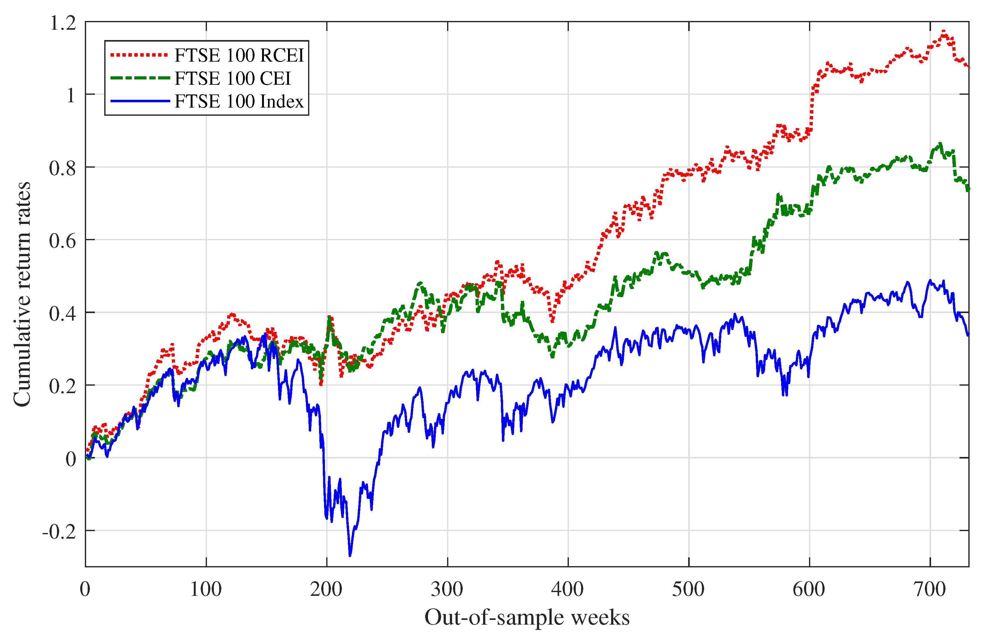
In practice, the primary concern is the out-of-sample performance of the determined portfolio. Therefore, we only demonstrate the out-of-sample results here. In the RCEI model, the lower semi-absolute tracking error thresholds $\alpha \left(s^1\right)$, $\alpha \left(s^2\right)$, $\alpha \left(s^3\right)$ are chosen as 0.007, 0.005, 0.003, respectively. The cardinality upper bounds are set to $K\left(s^1\right)=5$, $K\left(s^2\right)=10$, $K\left(s^3\right)=20$. That is to say, in a bull market, we prefer a more concentrated investment policy while we allow a larger tolerance of the losses under the index. In a bear market, we prefer a more diversified investment policy and set a smaller tolerance of the losses under the index, to reduce the risk. To elaborate whether the regime switching technique can improve the stability in enhanced indexation problems, we also test the cardinality constrained enhanced indexation model without regime switching, denoted by the CEI model for reference. We can obtain the optimal investment policy under the CEI model by solving the RCEI model with $J=1$, $\alpha \left(s^1\right)=\alpha$ and $K\left(s^1\right)=K$. For the CEI model, we set the threshold $\alpha =0.005$ and the cardinality upper bound $K=10$. All parameters in the partial penalty proximal ADMM are set as: the initial penalty parameter ${\mu }^1=2$, the initial penalty in ADMM ${\beta }^1=2$, the growth coefficient $\gamma =1.4$, the proximal coefficient $\sigma =1.3$, the external and internal tolerances are ${10}^{-5}$ and ${10}^{-3}$, respectively.

Figure 1 shows the out-of-sample cumulative return rates of the optimal tracking portfolios derived by the RCEI and CEI models in FTSE 100, compared with the cumulative return rates of the FTSE 100 index.

Figure 2 shows the out-of-sample cumulative return rates of the optimal tracking portfolios derived by the RCEI and CEI models in S&P 500, compared with the cumulative return rates of the S&P 500 index.

We can see from Figure 1 and Figure 2 that both optimal portfolios obtained from the RCEI and CEI models can efficiently track the trend of the market index and even outperform the market index. Meanwhile, the out-of-sample performances of the RCEI models are better than those of the CEI models or the indices in FTSE 100 and S&P 500 markets, respectively. The cumulative return rates of the optimal portfolios from the RCEI models are substantially higher than those from the CEI models and the market indices in UK and US financial markets. In addition, the optimal portfolios obtained from the RCEI model secure more stable returns and thus avoid substantial losses in a long-term investment process.

For more details, we show typical statistics of weekly return rates of out-of-sample portfolios as well as the average CPU time in

Table 3. Statistics of out-of-sample portfolio return rates of RCEI and CEI models.

Index	Model	Mean	Std	SR	MDD	${\mathbf{TE}}_{+}$	${\mathbf{TE}}_{-}$	Time(s)
FTSE 100	RCEI	0.0015	0.0158	0.0931	0.2522	0.0067	0.0057	1.07
	CEI	0.0010	0.0143	0.0709	0.5918	0.0063	0.0057	1.10
	Index	0.0005	0.0224	0.0209	0.7717	-	-	-
S&P 500	RCEI	0.0031	0.0220	0.1425	0.1986	0.0060	0.0038	18.79
	CEI	0.0014	0.0258	0.0553	0.2104	0.0041	0.0036	18.94
	Index	0.0009	0.0254	0.0364	0.6117	-	-	-

.

Table 3 shows that the means of the return rates of the RCEI and CEI models are much larger than that of the index, especially the RCEI model. In addition, the standard deviation of the RCEI and CEI models are smaller than that of the FTSE 100 index and close to that of the S&P 500 index, respectively. Sharpe ratio (SR) is a widely adopted indicator for calculating the risk-adjusted return, which can be used to evaluate a portfolio’s performance. We can see from Table 3 that, in both financial markets, the Sharpe ratio value of the optimal portfolios from the RCEI models are larger than those of the CEI models or the market indices, respectively. It means that, in terms of the risk-adjusted return, the RCEI model also outperforms the CEI model and the market index.

Considering the financial sustainability in the long run, we calculate the maximum drawdown (MDD) [32] for each optimal portfolio of each model and the index in FTSE 100 and S&P 500. MDD is the maximum loss from a peak to a trough of a portfolio before a new peak is attained. It is an indicator of downside risk over a specific time period. We can see from Table 3 that the MDD value of the RCEI model is obviously smaller than those of the CEI model and the market index. It means that, when we obtain excess returns by the RCEI model, we can simultaneously avoid heavy losses for more than ten years. It is very important for the financial sustainability. In particular, a heavy loss is a big blow for any investor, which will result in the unsustainability in financial investments.

Table 3 also reveals that the expectation of the positive part of the tracking error i.e., ${\mathrm{TE}}_{+}=\mathbb{E}[{(R^{\top }x-R_I)}_{+}]$, and the expectation of the negative part of the tracking error, i.e., ${\mathrm{TE}}_{-}=\mathbb{E}[{(R^{\top }x-R_I)}_{-}]$. In terms of ${\mathrm{TE}}_{+}$ and ${\mathrm{TE}}_{-}$, the performance of the RCEI model is better than that of the CEI model. Moreover, the proposed partial penalty proximal ADMM algorithm is highly efficient as the average CPU time is about 1 s in FTSE 100 enhanced problems and about 18 s in S&P 500 enhanced problems.

Furthermore, we divide the out-of-sample period of FTSE 100 and S&P 500 into three market regimes, respectively. Then, we compute the statistics of weekly return rates of the optimal portfolios under different market regimes, shown in

Table 4. Statistics of the out-of-sample return rates under different market regimes.

Index	Model	State	Mean	Std	SR	${\mathbf{TE}}_{+}$	${\mathbf{TE}}_{-}$
FTSE 100	RCEI	Bull	0.0030	0.0142	0.2149	0.0053	0.0058
		Consolidation	0.0015	0.0147	0.1006	0.0056	0.0051
		Bear	−0.0014	0.0202	−0.0678	0.0118	0.0068
	CEI	Bull	0.0025	0.0120	0.2114	0.0048	0.0058
		Consolidation	0.0003	0.0136	0.0243	0.0049	0.0056
		Bear	−0.0001	0.0191	−0.0058	0.0122	0.0059
	Index	Bull	0.0036	0.0187	0.1902	-	-
		Consolidation	0.0010	0.0195	0.0518	-	-
		Bear	−0.0063	0.0318	−0.3328	-	-
S&P 500	RCEI	Bull	0.0040	0.0184	0.2148	0.0031	0.0031
		Consolidation	0.0032	0.0241	0.1343	0.0055	0.0028
		Bear	0.0005	0.0253	0.0193	0.0158	0.0088
	CEI	Bull	0.0032	0.0206	0.1579	0.0033	0.0034
		Consolidation	0.0024	0.0235	0.1017	0.0045	0.0035
		Bear	−0.0056	0.0393	−0.1419	0.0059	0.0044
	Index	Bull	0.0033	0.0190	0.1731	-	-
		Consolidation	0.0014	0.0240	0.0591	-	-
		Bear	−0.0071	0.0396	−0.1803	-	-

.

In Table 4, we not only list the performance of the RCEI model under each market regime, but also that of the CEI model. We find that both RCEI and CEI models perform differently under different market regimes. Comparing with the CEI model, the RCEI model performs better in terms of the means, standard deviations and Sharpe ratios. In addition, the discrimination of the RCEI model in three market regimes are larger, which means that the RCEI model can describe the influence of different market regimes efficiently. In addition, in the bear market environment, the performance of the RECI model is better than that of the market index, which can avoid suffering a huge financial loss, and guarantee the sustainability of the investment consequently. It illustrates that the regime switching plays a fundamental role in financial sustainability.

Finally, we consider the effect of the cardinality constraint in the RCEI model. We test a reference of the RCEI model by removing the cardinality constraint, denoted by the REI model. We carry out the out-of-sample test for the REI model in a similar rolling forward way. Some statistics of out-of-sample weekly return rates of optimal portfolios determined by the RCEI and REI models are shown in

Table 5. Statistics of out-of-sample return rates of RCEI and REI models.

Index	Model	Mean	Std	SR	${\mathbf{TE}}_{+}$	${\mathbf{TE}}_{-}$	Stocks	Time(s)
FTSE 100	RCEI	0.0015	0.0158	0.0931	0.0067	0.0057	9.36	1.07
	REI	0.0017	0.0173	0.0974	0.0071	0.0061	88.75	0.06
S&P 500	RCEI	0.0031	0.0220	0.1425	0.0060	0.0038	9.67	18.79
	REI	0.0036	0.0282	0.1277	0.0104	0.0083	383.17	0.83

. The average number of actually invested stocks in the corresponding optimal portfolios as well as the average CPU time are also shown in Table 5.

We can observe from Table 5 that, comparing with the REI model, the optimal portfolio obtained from the RCEI model could significantly reduce the number of really invested stocks without losing too much performance. Limiting the number of actually invested stocks is crucial in financial management due to the following reasons. Firstly, the transaction cost is high relative to the number of stocks we buy or sell. If we reduce the number of stocks in the indexation portfolio, we can save much capital in the transaction cost. Secondly, as fund managers or individual investors, it is impossible for them to manage dozens or hundreds of stocks at the same time, which can be regarded as another kind of manpower cost. This further proves that the RCEI model is sustainable in long-term financial investment problems if we take transaction costs into account.

The average CPU time shows that the computational cost of the REI model is lower than that of the RCEI model. The reason is that we need to introduce some auxiliary variables and extra computation for dealing with the cardinality constraint, which not only increase the dimension of the problem but also increase the number of iterations for obtaining the optimal solution. Fortunately, the computation time of the RCEI model is quite acceptable even if we deal with 500 constituent stocks in the S&P 500 case.

5. Conclusions

In this paper, we propose a new sustainability-oriented enhanced indexation model with regime switching and cardinality constraint. By adopting the regime switching technique, we can flexibly set different risk thresholdsbenchmarks and cardinality bounds in different market environments, which can mirror the fluctuation of market environment in a timely manner. We solve the resulting deterministic optimization problem by the partial penalty proximal ADMM, which can deal with the cardinality constraint optimization problem in an acceptable computation time. In addition, we examine the performance of the proposed RCEI model in different financial markets and compare the out-of-sample results with FTSE 100 and S&P 500 indices, respectively. The numerical results show that the optimal portfolios obtained from the RCEI model have higher accumulative return and lower risk compared with those obtained from the CEI model and the market indices in the long-term investment process. At the same time, the invested stocks can be streamlined without losing much performance by adopting our proposed model and algorithm.

This innovative work fuels our conviction that the proposed model and algorithm are highly compatible with sustainable strategies, and investors can reap significant benefits from their joint cooperation. The accumulating evidence about the benefits of investment strategies would cultivate the growth of a sustainable investing market. Firstly, fund managers and individual investors can choose different threshold parameters and cardinality bounds in various financial markets. Risk-preference investors can set the semi-absolute tracking error threshold larger for higher excess returns. Risk-aversion ones who pursue a more secure return can set the threshold smaller. Fund managers and individual investors can also adjust the cardinality bounds according to their needs. Based on our experiences, cardinality bounds are suggested as no more than 20 for fund mangers and no more than 10 for individual investors. Secondly, our proposed model is more effective in mature financial markets. It should be used with caution in emerging financial markets which are less effective. To speak plainly, arbitrage opportunities will often occur in emerging markets; therefore, the optimal value may go to infinity. However, this is not consistent with the facts. In addition, mature financial markets provide more products that can be taken into account in our portfolios, such that investors can still maintain positive income by holding some short positions when the market is slow. In general, our method echoes sustainable growth in long-term investment processes.

This work can further be improved such as using another tracking error measure instead of the lower semi-absolute measure or extending the model to the multi-period case. These promising topics are left for future research.