Specification Testing of Production in a Stochastic Frontier Model

Abstract

Parametric production frontier functions are frequently used in stochastic frontier models, but there do not seem to be any empirical test statistics for the plausibility of this application. In this paper, we develop procedures to test whether or not the parametric production frontier functions are suitable. Toward this aim, we developed two test statistics based on local smoothing and an empirical process, respectively. Residual-based wild bootstrap versions of these two test statistics are also suggested. The distributions of technical inefficiency and the noise term are not specified, which allows specification testing of the production frontier function even under heteroscedasticity. Simulation studies and a real data example are presented to examine the finite sample sizes and powers of the test statistics. The theory developed in this paper is useful for production managers in their decisions on production.

1. Introduction

Since the seminal works of [1,2], stochastic frontier analysis (SFA) has been a very appealing and popular approach for studying productivity and efficiency analysis. Greene [3] extended the stochastic frontier model by allowing the one-sided component of the disturbance to have a two-parameter gamma distribution rather than the less-flexible half-normal distribution. Greene [4] extended the model further by using a nonlinear specification. For an up-to-date introduction and literature review, see [5,6].

Consider the following SFA model:

$$\begin{array}{c}\hfill Y=m\left(X\right)-U+V,\end{array}$$

(1)

where Y is the log of output, X is the log of inputs of dimension p, $m(·)$ is an unknown smooth production frontier function, U is the inefficiency term, and V represents random noise. Assume that the positive random variable, U, and the symmetric noise term, V, are conditionally independent, given the inputs X, and $E\left(V\right|X)=0$.

Parametric SFA models specify the functional form of the production frontier function, $m(·)$, as well as the distributions of the inefficiency term, U, and the independent noise, V. A fully parametric SFA framework sacrifices flexibility, and has been criticized as a major deficiency of SFA models (see details in [7]).

Some authors have discussed how to test the distributional assumptions on U and/or V. For instance, Wang et al. [8] developed the Pearson ${\chi }^2$ and Kolmogorov–Smirnov tests for the distribution of U. Chen et al. [9] proposed a centered residuals-based method of moments to test the distributional assumptions on both U and V (see also [10,11,12,13]). However, it should be noted that all these procedures are based on the assumed parametric form of the production frontier function. If the parametric assumption on $m(·)$ is not valid, the conclusions can be inaccurate and misleading.

On the other hand, there have been attempts to reduce the parametric restrictions on the production frontier function. Fan et al. [14] introduced the quasi-likelihood method, where the production frontier is not specified, but distributional assumptions are imposed on the stochastic components. Kumbhakar et al. [15] proposed a local maximum likelihood method but without parametric assumptions on the production frontier function, while using semi-parametric assumptions about U and V.

Recently, Simar et al. [16] developed a nonparametric least squares method to avoid the high computational complexity involved in the local maximum likelihood method in [15]. Another merit of the method of [16] is that only local distributional assumptions on U are needed, although symmetry is still necessary for V. Nonetheless, it should be realized that the methods discussed above would not be necessary if the hypothetical parametric model was satisfied. Studying the “wrong skewness phenomenon” in stochastic frontiers (SF), Bonanno et al. [17] proposed a more general and flexible specification of the SF model by introducing dependences between the two error components and asymmetry of the random error.

The studies discussed above call for the specification testing of the production frontier function. Parametric specifications for the frontier are appealing because they offer easy economic interpretation of the production process. Furthermore, due to well-established theories, easy computation, and interpretation, parametric SFA models have been dominant in the area of productivity and efficiency analysis. Specification testing can also be used to validate the accuracy of some production theory, such as Cobb–Douglas, CES, Translog, and related functions. There is literature on specification testing for conventional regression models (see [18] for a useful review). However, it would seem that there is as of yet no analysis that discusses this problem for SFA models.

In this paper, we aim to develop procedures to test whether the production frontier function can be described by some known parametric functions. To be precise, the null hypothesis is given as:

$$\begin{array}{c}\hfill H_0:m\left(X\right)=g(X,{\beta }_0),\end{array}$$

(2)

for some ${\beta }_0$ against the alternative hypothesis:

$$\begin{array}{c}\hfill H_1:m\left(X\right)\ne g(X,\beta ),\end{array}$$

(3)

for any $\beta$, where $g(X,\beta )$ is a known smooth function with unknown d-dimensional parameter $\beta$.

Two test statistics are proposed, based on local smoothing and global smoothing, respectively. To apply these two test statistics in practice, we suggest the residual-based wild bootstrap. A merit of our procedure is that, even under heteroscedasticity, the test statistics can still detect the alternative hypothesis efficiently. To the best of our knowledge, this is a novel contribution to the literature. The theory developed in this paper is useful for production managers in their decisions on production [19].

The remainder of the paper is organized as follows. In Section 2, we construct the test statistics and describe the residual-based wild bootstrap. In Section 3, simulation results are reported to examine the finite sample performance of the test statistics. An empirical application is given in Section 4, and Section 5 concludes the paper.

2. Test Statistics

To focus on specification testing of the production frontier function, we first discuss the estimation procedures for the parametric SFA model without specific distributional assumptions on U and V.

2.1. Estimation

Let ${\mu }_U\left(X\right)=E\left(U\right|X)$, $ϵ=V-U+{\mu }_U\left(X\right)$, and $r_1\left(X\right)=Y-ϵ$. Note that $E\left(ϵ\right|X)=0$ always holds. We can then rewrite model (1) under the null hypothesis as follows:

$$Y^1=Y+{\mu }_U\left(X\right)=g(X,\beta )+ϵ.$$

For the data set $(Y^1,X)$, the model is the traditional parametric regression model. If we can obtain the value of ${\mu }_U\left(X\right)$, then we can estimate the parameter $\beta$ by using nonlinear least squares based on $(Y^1,X)$. Thus, the most important and difficult part is how to estimate ${\mu }_U\left(X\right)$. To achieve this goal, we adopt the approach that was recently proposed by [16].

Under the null hypothesis, model (1) can also be rewritten as:

$$Y=r_1\left(X\right)+ϵ,$$

where $E\left(ϵ\right|X)=0$ still holds, which is the standard nonparametric regression model. We can obtain the estimator of $r_1\left(X\right)$, ${\widehat{r}}_1\left(X\right)$, by using nonparametric methods such as kernels, local polynomials, and/or splines. Although there are several nonparametric methods for regression models, in the following we focus on kernel-type estimators given by ${\widehat{r}}_1\left(x\right)={\sum }_{i=1}^n{W}_{ni}\left(x\right)Y_i$, with:

$$W_{ni}\left(x\right)=\frac{K_h(x-X_i)}{{\sum }_{j=1}^n{K}_h(x-X_j)},$$

and $K_h(·)$ = $K(·/h)/h^p$, with $K(·)$ the kernel function, and h being the bandwidth.

Under the symmetry assumption on V, and the conditional independence of U and V given X, we have the following:

$$\begin{array}{ccc}\hfill E\left({ϵ}^2\right|X)& =& va{r}_U\left(X\right)+va{r}_V\left(X\right),\hfill \\ \hfill E\left({ϵ}^3\right|X)& =& -E\left[{(U-{\mu }_U\left(X\right))}^3\right|X],\hfill \end{array}$$

where $va{r}_U\left(X\right)$ and $va{r}_V\left(X\right)$ denote the conditional variances of U and V given X, respectively.

Denote $r_j\left(X\right)=E\left({ϵ}^j\right|X)$ for $j=2$ and 3. After estimation of $r_1\left(X\right)$, we can obtain the residuals, $\widehat{ϵ}=Y-{\widehat{r}}_1\left(X\right)$. By adopting appropriate nonparametric techniques, we can estimate the functions $r_j\left(X\right)$ for $j=2$ and 3 consistently. Define:

$${\widehat{r}}_j\left(x\right)=\sum _{i=1}^n{W}_{ni}\left(x\right){(Y-{\widehat{r}}_1\left(X_i\right))}^j,$$

for $j=2$ and 3. Note that if ${\mu }_U\left(X\right)$ is a function of $E\left[{(U-{\mu }_U\left(X\right))}^3\right|X]$, then we can easily estimate ${\widehat{r}}_3\left(X\right)$. To achieve this goal, local parametric assumptions on the types of distributions of $U|x$ are necessary.

Assume that $U|x\sim |N(0,{\sigma }_U^2\left(x\right))|$ and that, conditionally on X, U and V are independent, which is the same paradigm as in [15]. As a result, we have:

$$\begin{array}{ccc}\hfill {\mu }_U\left(X\right)& =& E\left(U\right|X)=\sqrt{\frac{2}{\pi }}{\sigma }_U\left(X\right),\hfill \\ \hfill E\left({ϵ}^2\right|X)& =& \frac{\pi -2}{\pi }{\sigma }_U^2\left(X\right)+va{r}_V\left(X\right),\hfill \\ \hfill E\left({ϵ}^3\right|X)& =& \sqrt{\frac{2}{\pi }}\left(1-\frac{4}{\pi }\right){\sigma }_U^3\left(X\right)\le 0.\hfill \end{array}$$

From the above equations, we can obtain the following:

$$\begin{array}{ccc}\hfill {\widehat{\sigma }}_U\left(X\right)& =& max\left\{0,{\left[\sqrt{\frac{\pi }{2}}\left(\frac{\pi }{\pi -4}\right)\widehat{E}\left({ϵ}^3\right|X)\right]}^{1/3}\right\},\hfill \\ \hfill {\widehat{\mu }}_U\left(X\right)& =& \sqrt{\frac{2}{\pi }}{\widehat{\sigma }}_U\left(X\right)\hfill \end{array}$$

(for further details, see [16]).

After estimating ${\widehat{\mu }}_U\left(X\right)$, we can estimate $\beta$ by using nonlinear least squares based on the data points, $\left\{({\widehat{Y}}_i^1,X_i)\right|i=1,\cdots ,n\}$. Defining ${\widehat{Y}}_i^1=Y_i+{\widehat{\mu }}_U\left(X_i\right)$, let ${ϵ}_0=Y^1-g(X,\beta )$ to obtain the residuals under the null hypothesis, ${\widehat{ϵ}}_{0i}={\widehat{Y}}_i^1-g(X_i,\widehat{\beta })$.

2.2. Construction

Under the null hypothesis, we can easily obtain:

$$E\left({ϵ}_0\right|X)=E(Y+{\mu }_U\left(X\right)-g(X,\beta )|X)=E(g(X,\beta )+V-U+{\mu }_U\left(X\right)-g(X,\beta )|X)=0,$$

while under the alternative hypothesis, we obtain:

$$\begin{array}{ccc}\hfill E\left({ϵ}_0\right|X)& =& E(Y+{\mu }_U\left(X\right)-g(X,\beta )|X)=E(m\left(X\right)+V-U+{\mu }_U\left(X\right)-g(X,\beta )|X)\hfill \\ & =& m\left(X\right)-g(X,\beta )\ne 0.\hfill \end{array}$$

The above observations form the basis of the construction of the new test statistics. We introduce the local smoothing-based test statistic. Note that under the null hypothesis, we have:

$$E\left({ϵ}_{0}E\left({ϵ}_0\right|X)f\left(X\right)\right)=E\left[E^2\left({ϵ}_0\right|X)f\left(X\right)\right]=0,$$

where $f\left(X\right)$ is the density function of X. Under the alternative hypothesis, the first term in the above equation must be positive. Thus, the empirical counterpart of this term can be used as the test statistic. By using the leave-one-out kernel estimator of $f\left(X\right)$ and $E\left({ϵ}_0\right|X)$, the following test statistic is constructed:

$$\begin{array}{ccc}\hfill T_{n1}& =& \frac{1}{n(n-1)}\sum _{i=1}^n\sum _{j\ne i}^n{K}_h(X_i-X_j){\widehat{ϵ}}_{0i}{\widehat{ϵ}}_{0j}.\hfill \end{array}$$

The type of test statistic given above is introduced in [20], and was proposed independently by [21]. In classical regression models, it can be shown that the distribution of $T_{n1}$ converges to a centered normal as $n\to \infty$. However, we should note that in the context of the SFA model, the asymptotic properties of $T_{n1}$ can be complex due to the existence of the term ${\mu }_U\left(X\right)$. To formally study the asymptotic properties of $T_{n1}$, we need to investigate the impact of the nonparametric estimation of ${\widehat{\mu }}_U\left(X\right)$ on the estimation of $\beta$ explicitly. In this paper, we focus on investigating the numerical performance of $T_{n1}$, and leave the theoretical project for future research.

We can construct an empirically-based test statistic. Note that under the null hypothesis, the following equation holds:

$$E\left({ϵ}_{0}I(X\le x)\right)=0,\forall x\in {\mathbb{R}}^p.$$

This motivates the construction of the residual-based empirical process, as follows:

$$\begin{array}{ccc}\hfill R_n\left(x\right)& =& \frac{1}{\sqrt{n}}\sum _{i=1}^n{\widehat{ϵ}}_{0i}I(X_i\le x).\hfill \end{array}$$

Then, the Cramér–von Mises-type test statistic can be defined by:

$$\begin{array}{c}\hfill T_{n2}=\int {\left(R_n\left(x\right)\right)}^{2}d{F}_n\left(x\right),\end{array}$$

(4)

where $F_n\left(x\right)$ is the empirical distribution based on {$X_1,X_2,\cdots ,X_n$}.

Similarly, in classical regression models, it can be shown that the defined empirical process $R_n\left(x\right)$ converges to a centered continuous Gaussian process, and the test statistic converges to the functional of this Gaussian process (see details in [22]), but the covariance function of the Gaussian process would be changed. We leave the formal theoretical analysis for future research.

We follow the residual-based wild bootstrap method (see details in [23]) to determine whether to reject the null hypothesis using the following steps:

Step 1.

Obtain ${\widehat{\mu }}_U\left(X\right)$, $\widehat{\beta }$, and ${\widehat{ϵ}}_0$ by using the approach proposed in Section 2.1, and then construct $T_{ni},i=1,2$, as in Section 2.2.

Step 2.

Generate bootstrap observations, $Y_i^{*}=g(X_i,\widehat{\beta })-{\widehat{\mu }}_U\left(X_i\right)+{\widehat{ϵ}}_{0i}\times e_i$. Here ${\left\{e_i\right\}}_{i=1}^n$ is a sequence of i.i.d. random variables with zero mean, unit variance, and independent of the sequence ${\{Y_i,X_i\}}_{i=1}^n$. Usually, ${\left\{e_i\right\}}_{i=1}^n$ can be chosen to be i.i.d. Bernoulli variates with:

$$P(e_i=\frac{1-\sqrt{5}}{2})=\frac{1+\sqrt{5}}{2\sqrt{5}},P(e_i=\frac{1+\sqrt{5}}{2})=1-\frac{1+\sqrt{5}}{2\sqrt{5}}.$$

Step 3.

Let $T_{ni}^{*},i=1,2$ be defined similarly as $T_{ni},i=1,2$, based on the bootstrap sample, ${\{Y_i^{*},X_i\}}_{i=1}^n$.

Step 4.

Repeat Steps 2 and 3, B times, and calculate the p-value as $p_i^B=\#\{T_{ni}^{*}>T_{ni}\}/B$.

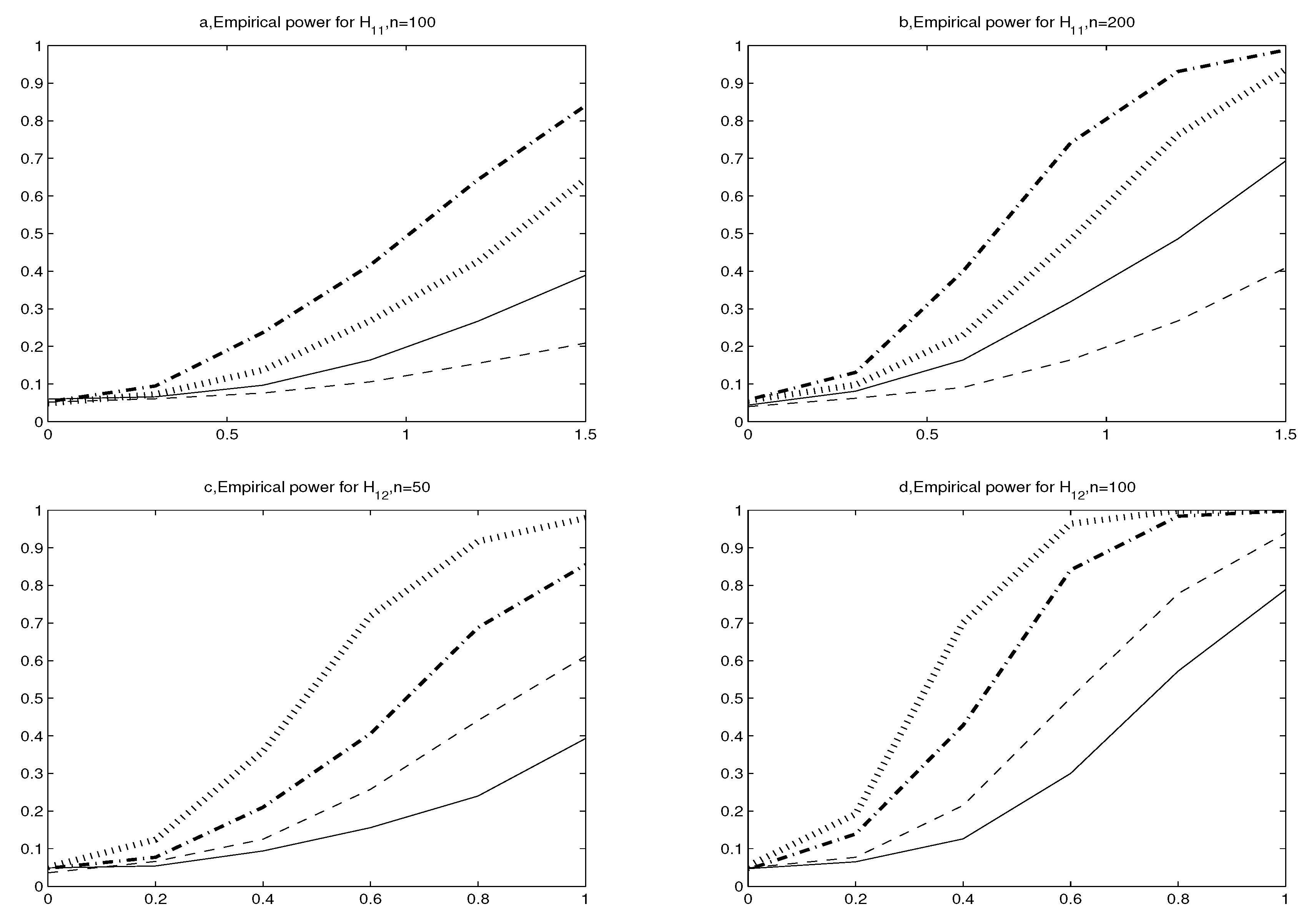
3. Simulations

We now perform simulations to examine the finite sample performance of the proposed test statistics.

Study 1

$$\begin{array}{c}{H}_{11}:Y=5+5X+aexp\left\{X^2\right\}-U+V,\hfill \\ H_{12}:Y=5+5X+asin\left\{4\pi X\right\}-U+V.\hfill \end{array}$$

The value $a=0$ corresponds to the null hypothesis, and $a\ne 0$ to the alternative. In the above models, we take $X\sim U(0,1)$, $U\sim \left|N\right(0,1\left)\right|$, and $V\sim N(0,{\sigma }_V^2)$, where ${\sigma }_V=0.75\times \sqrt{(\pi -2)/\pi }$. For the models, under the null hypothesis, $a=0$, this is Example 1 in [15]. For $H_{11}$, the sample size is taken to be 100, and $a=\{0.0,0.3,\cdots ,1.5$} to examine the size and power performance of the proposed test statistics, $T_{n1}$ and $T_{n2}$. For $H_{12}$, we consider $n=50$ and 100, and the sequence of a is taken to be $a=\{0.0,0.2,\cdots ,1.0\}$.

In the simulation study, the number of replications was 2000. For each replication, $B=500$ bootstrapped samples were generated. In the nonparametric regression estimation, the kernel function was taken to be $K\left(u\right)=15/16{(1-u^2)}^2$, if $\left|u\right|\le 1$; and 0, otherwise. The bandwidth was taken to be $h=\widehat{\sigma }\left(X\right)\times n^{-1/5}$ for simplicity, where $\widehat{\sigma }\left(X\right)$ is the empirical estimator of the standard deviation of X. The nominal level of $\alpha$ was set at 0.05.

The simulation results are presented in

Table 1. Simulated sizes and powers of the proposed test statistics $T_{n1}$ and $T_{n2}$ for Study 1.

${\mathit{H}}_{11}$	$\mathit{n}=100$
$\mathit{a}$	${\mathit{T}}_{\mathit{n}\mathbf{1}}$		${\mathit{T}}_{\mathit{n}\mathbf{2}}$
0.0	0.0490		0.0530
0.3	0.0730		0.0950
0.6	0.1370		0.2370
0.9	0.2685		0.4170
1.2	0.4255		0.6430
1.5	0.6445		0.8400
${\mathit{H}}_{\mathbf{12}}$	$\mathit{n}=\mathbf{50}$		$\mathit{n}=\mathbf{100}$
$\mathit{a}$	${\mathit{T}}_{\mathit{n}\mathbf{1}}$	${\mathit{T}}_{\mathit{n}\mathbf{2}}$	${\mathit{T}}_{\mathit{n}\mathbf{1}}$	${\mathit{T}}_{\mathit{n}\mathbf{2}}$
0.0	0.0510	0.0480	0.0540	0.0450
0.2	0.1240	0.0770	0.1920	0.1390
0.4	0.3590	0.2100	0.7010	0.4280
0.6	0.7190	0.4060	0.9640	0.8410
0.8	0.9170	0.6880	0.9990	0.9840
1.0	0.9790	0.8550	1.0000	0.9980

.

From the table, we have the following observations. First, for all situations considered, the empirical sizes of the two test statistics were all close to the nominal level. This implies that the proposed test statistics had accurate size. Second, when we consider empirical power, we can see clearly that the proposed tests were very sensitive to the alternative, such that when the value of a increased, power increased quickly. For model $H_{11}$, the second test statistic, $T_{n2}$, had higher power than the first test statistic, $T_{n1}$. However, for $H_{12}$, $T_{n1}$ was more powerful. For model $H_{12}$, when the sample size was $n=100$, the power performance of both tests improved compared with sample size $n=50$.

Study 2

Consider the same models as in Study 1, but now introduce heteroscedasticity in the distribution of the technical inefficiency. Here, we have $U|X=x\sim |N(0,{(1+x)}^2)|$. We should note that under the null hypothesis, $a=0$, is Example 2 in [15]. This study investigates the impact of heteroscedasticity on the performance of the two proposed test statistics. Other settings are the same as in Study 1.

The simulation results are shown in Figure 1. For comparison, we also plot the simulation results of these two test statistics in Study 1.

From this figure, we conclude that the powers of the two test statistics decreased significantly compared with the results in Study 1. This suggests that heteroscedasticity in the distribution of the technical inefficiency can have a negative impact on power performance. We can also see that for $H_{11}$, $T_{n2}$ performed better than $T_{n1}$, while for $H_{12}$, $T_{n1}$ was more powerful. These observations suggest that the two new test statistics should be viewed as complementary to each other.

4. Empirical Application

A rice production data set is available online, as described in the Preface of [24] (p. xvi, further details on the data can be found in Appendix 2 of [24]). The data set was recently analyzed in [8] to calculate goodness-of-fit tests for the distribution of technical inefficiency. Here we use this data set to check whether the Cobb–Douglas model is plausible.

Following [8,24], three inputs (area, labor, and fertilizer) and one output (tons of freshly threshed rice) were used, denoted by $X=(X_1,X_2,X_3)=(AREA,LABOR,NPK)$, and $Y=PROD$, respectively. The Cobb–Douglas model is given as follows:

$$lnY={\beta }_0+\sum _{i=1}^3{\beta }_{i}ln{X}_i-U+V.$$

In our context, the null hypothesis is:

$$H_0:m\left(X\right)={\beta }_0+\sum _{i=1}^3{\beta }_{i}ln{X}_i.$$

For sample size $n=344$, the values of $T_{ni},i=1,2$, were 1.8062 and 616.5035, and the corresponding p-values were 0.160 and 0.774, respectively. Since both p-values were larger than 0.05, a Cobb–Douglas model is plausible. This implies that for the data set we used in our illustration, the relationship between the log output and log inputs can be considered as linear.

5. Concluding Remarks

Though SFA models have been used widely in many disciplines (e.g., economics, finance, and statistics), a formal specification testing procedure for the production frontier function has not been available. This paper develops two new test statistics by adopting local smoothing and global smoothing methods, respectively.

The asymptotic properties of the two test statistics under the null hypothesis, fixed alternative hypothesis, and local alternative hypothesis have not been investigated. The existence of the inefficiency term, U, makes the analysis complicated. We leave these interesting and important theoretical studies to future research.

Without explicit asymptotic distributions under the null hypothesis, we must rely on resampling approaches to calibrate the critical values. To this end, the residual-based wild bootstrap is suggested. The new proposed test statistics allow specification testing of the production frontier function, even under heteroscedasticity. The simulation studies showed that the sizes of the two test statistics are quite close to the nominal level, and that the powers are also satisfactory—even when the sample size is relatively small ($n=50$). The theory developed in this paper is useful for production managers (see details in [25,26,27]) in their decisions on production [19] and for investors [28] in their decision making in their investment.

Model building is always a key concern for theoretical and practical studies. In this paper, we investigate whether a parametric production frontier function is suitable in the analysis. Lai et al. [29] considered the model selection criterion for the stochastic frontier models. Later on, Lai et al. [30] suggested using the model-averaged estimator based on the multimodel inference to estimate stochastic frontier models. Parmeter et al. [31] also suggested the use of this approach.

References

- Aigner, D.J.; Lovell, C.A.K.; Schmidt, P. Formulation and estimation of stochastic frontier models. J. Econom. 1977, 6, 21–37. [Google Scholar] [CrossRef]
- Meeusen, W.; Broeck, J.V.D. Efficiency estimation from Cobb-Douglas production functions with composed error. Int. Econ. Rev. 1977, 18, 435–444. [Google Scholar] [CrossRef]
- Greene, W.H. A Gamma-distributed stochastic frontier model. J. Econom. 1990, 46, 141–163. [Google Scholar] [CrossRef] [Green Version]
- Greene, W.H. Reconsidering heterogeneity in panel data estimators of the stochastic frontier model. J. Econom. 2005, 126, 269–303. [Google Scholar] [CrossRef]
- Kumbhakar, S.; Lovell, C.A.K. Stochastic Frontier Analysis; Cambridge University Press: Cambridge, UK, 2000. [Google Scholar]
- Fried, H.; Lovell, C.A.K.; Schmidt, S. The Measurement of Productive Efficiency and Productivity Change; Oxford University Press: New York, NY, USA, 2008. [Google Scholar]
- Simar, L.; Wilson, P. Statistical approaches for nonparametric frontier models: A guided tour. Int. Stat. Rev. 2015, 83, 77–110. [Google Scholar] [CrossRef]
- Wang, W.S.; Amsler, C.; Schmidt, P. Goodness of fit tests in stochastic frontier models. J. Prod. Anal. 2011, 35, 95–118. [Google Scholar] [CrossRef]
- Chen, Y.T.; Wang, H.J. Centered-residuals-based moment tests for stochastic frontier models. Econom. Rev. 2012, 31, 625–653. [Google Scholar] [CrossRef]
- Schmidt, P.; Lin, T.F. Simple tests of alternative specifications in stochastic frontier models. J. Econom. 1984, 24, 349–361. [Google Scholar] [CrossRef]
- Coelli, T.J. Estimators and hypothesis tests for a stochastic frontier function: A Monte Carlo analysis. J. Prod. Anal. 1995, 6, 247–268. [Google Scholar] [CrossRef]
- Lee, L.F. A test for distributional assumptions for the stochastic frontier functions. J. Econom. 1983, 22, 245–267. [Google Scholar] [CrossRef]
- Kopp, R.J.; Mullahy, J. Moment-based estimation and testing of stochastic frontier models. J. Econom. 1990, 46, 165–183. [Google Scholar] [CrossRef]
- Fan, Y.; Li, Q.; Weersink, A. Semiparametric estimation of stochastic production frontier. J. Bus. Econ. Stat. 1996, 14, 460–468. [Google Scholar]
- Kumbhakar, S.C.; Park, B.U.; Simar, L.; Tsionas, E.G. Nonparametric stochastic frontiers: A local likelihood approach. J. Econom. 2007, 137, 1–27. [Google Scholar] [CrossRef]
- Simar, L.; Van Keilegom, I.; Zelenyuk, V. Nonparametric least squares methods for stochastic frontier models. J. Prod. Anal. 2017, 47, 189–204. [Google Scholar] [CrossRef]
- Bonanno, G.; De Giovanni, D.; Domma, F. The ‘wrong skewness’ problem: A re-specification of stochastic frontiers. J. Prod. Anal. 2017, 47, 9–64. [Google Scholar] [CrossRef]
- González-Manteiga, W.; Crujeiras, R.M. An updated review of goodness-of-fit tests for regression models. Test 2013, 22, 361–411. [Google Scholar] [CrossRef]
- Tsekouras, K.; Chatzistamoulou, N.; Kounetas, K. Productive performance, technology heterogeneity and hierarchies: Who to compare with whom. Int. J. Prod. Econ. 2017, 193, 465–478. [Google Scholar] [CrossRef]
- Zheng, J.X. A consistent test of functional form via nonparametric estimation techniques. J. Econom. 1996, 75, 263–289. [Google Scholar] [CrossRef]
- Fan, Y.; Li, Q. Consistent model specification tests: Omitted variables and semiparametric functional forms. Econometrica 1996, 64, 865–890. [Google Scholar] [CrossRef]
- Stute, W. Nonparametric model checks for regression. Ann. Stat. 1997, 25, 613–641. [Google Scholar]
- Stute, W.; Gonzáles-Manteiga, W.; Presedo-Quindimil, M. Bootstrap approximation in model checks for regression. J. Am. Stat. Assoc. 1998, 93, 141–149. [Google Scholar] [CrossRef]
- Coelli, T.J.; Prasada Rao, D.S.; O’Donnell, C.J.; Battese, G.E. An Introduction to Efficiency and Productivity Analysis, 2nd ed.; Springer: New York, NY, USA, 2005. [Google Scholar]
- Guo, X.; Wong, W.K.; Xu, Q.F.; Zhu, L.X. Production and hedging decisions under regret aversion. Econ. Model. 2015, 51, 153–158. [Google Scholar] [CrossRef]
- Moslehpour, M.; Pham, V.K.; Wong, W.K.; Bilgicli, I. E-purchase intention of Taiwanese consumers: Sustainable mediation of perceived usefulness and perceived ease of use. Sustainability 2018, 10, 234. [Google Scholar] [CrossRef]
- Li, C.S.; Wong, W.K.; Peng, S.C.; Tsendsuren, S. The effects of health status on life insurance holding in 16 European countries. Sustainability 2018, in press. [Google Scholar]
- Li, Z.; Li, X.; Hui, Y.C.; Wong, W.K. Maslow portfolio selection for individuals with low financial sustainability. Sustainability 2018, 10, 1128. [Google Scholar] [CrossRef]
- Lai, H.P.; Huang, C.J. Likelihood ratio tests for model selection of stochastic frontier models. J. Prod. Anal. 2010, 34, 3–13. [Google Scholar] [CrossRef]
- Lai, H.P.; Huang, C.J. Estimation of stochastic frontier models based on multimodel inference. J. Prod. Anal. 2012, 38, 273–284. [Google Scholar]
- Parmeter, C.F.; Wan, A.T.; Zhang, X.Y. Model Averaging Estimators for the Stochastic Frontier Model, Working Paper. 2016. Available online: https://www.bus.miami.edu/_assets/files/repec/WP2016-09.pdf (accessed on 27 July 2018).