Regime-Switching Determinants for Spreads of Emerging Markets Sovereign Credit Default Swaps

Abstract

Using the Markov regime switching approach, we investigate the dependency of short term sovereign credit default swap (SCDS) spread changes on a nation’s country-specific fundamental factors, local, regional and macroeconomic global factors. We find that the significance of the determinants of SCDS spread changes differ across the two states of our regime-switching model. Specifically, in the good state, the weekly SCDS spread changes are mainly determined by local, regional and fundamental factors; whereas global variables have a stronger influence in the bad regime. In particular, US market returns play a dominant role in influencing the SCDS spread change in the bad state suggesting loss aversion and flight–to–quality behavior of investors. We then examine the cross-sectional differences of the above regime switching effect based on country-specific characters and find that the regime switching effect is associated with a nation’s country-specific characters such as openness, economic size and so forth.

1. Introduction

The sovereign default of Greece and the ongoing credit crisis in the Euro Zone have raised people’s concern on sovereign credit risk. Sovereign credit risk is determined by the country’s ability and willingness to re-pay its debt owing to creditors and is reflected in the spread paid for protection offered by the corresponding Sovereign Credit Default Swap (SCDS). Credit risk indicated by a nation’s SCDS spread essentially reflects the same fundamental economic condition and market information as the yield of the underlying government bonds. SCDS spread is considered to be a timelier measure of sovereign credit risk than government bond yield spread. Adler and Song [1] compare the behavior of emerging market SCDS spreads and the corresponding bond yields and reject the widely accepted parity relationship between SCDS spreads and bond yields in the literature. Ammer and Cai [2] examine the relationship between SCDS spreads and bond yields for nine emerging market sovereigns and find that these two measures of credit risk deviate significantly in the short run with the former leading the later in price discovery [3]. They attribute such deviation to the higher liquidity in trading of SCDS.

In this paper, we examine the deterministic factors that affect the variation of a nation’s credit risk as captured by its short-term SCDS spread changes using Markov regime switching model. We focus on the sovereign credit market of emerging nations which are by far the most liquid. Evidence shows that the SCDS spread changes are affected by different factors in different economic and market conditions and cannot be fully explained by country specific economic fundamental variables [4,5,6]. Other than country specific economic fundamental variables global factors do play a significant role in influencing the sovereign risk of emerging countries. There are two possible channels through which global factors may exert their influence. First of all, the global effect could be the result of the fundamental economic relation between the emerging country and its global trading partners. Second, it may as well be through the actions in the international financial markets. We expect to witness an elevation of the sovereign risk of an emerging nation if foreign investors lose their appetite on the local financial assets. This type of global effect is expected to be time varying with the effect being more salient during the downturn and/or volatile market condition, in which the market is more prone to a flight-to-quality phenomenon. None of the above-mentioned studies explores the determinants of sovereign credit risk in a state-contingent framework.

Our study contributes to the literature by examining how the influence of different factors may vary in different states of the markets using Markov regime switching model. In particular, rather than classifying the state based on exogenous information that may not be directly relevant to the SCDS market, we let the data to speak for themselves by using the Markov regime switching model to identify the good versus the bad states of the market. This study is one of the most comprehensive empirical studies on SCDS covering a total of 11 emerging market countries across different geographical regions and at different stage of economic development. The time period under investigation is also one of the longest in the literature.

Markov regime switching model is used in a variety of economic and finance research. Goldfeld and Quandt [7] introduce the Markov model for switching regressions in the econometric analysis. Cosslett and Lee [8] use Markov switching in their discrete time models. Hamilton [9] applies Markov switching model to explain the dependence of real output growth on business cycle. In a subsequent paper, Hamilton [10] formally develops the statistical representation to use discrete-time and discrete-space Markov chain to model the transition of unobservable regime switching states in time series data. Since then, the Markov switching framework is widely exploited in a number of studies to model different financial time series that exhibit regime varying effect. For example, previous research uses it to examine stock market returns [11,12,13,14]. Clarida et al. [15] investigate the regime shifting effect in the term structure of interest rates. From our knowledge, regime switching model has not been used to study the time series behavior of SCDS. The use of the regime switching model allows us to capture the potential state-contingent behavior of SCDS spread allowing for the influence of different explanatory variables to vary under different economic and market conditions.

In analyzing the regime switching effect of the explanatory variables we also witness a significant difference among the countries in terms of the extent of which these explanatory variables are associated with a country’s SCDS spread change. To identify the determinants of these cross-sectional differences we conduct a cross sectional analysis to investigate the variation of the significance of explanatory variables across several categories of sub-groups of our sample of emerging market countries. We expect that the more open an economy and the more it is integrated to the global economy, the stronger will be the influence of regional and global factors on its SCDS spread change. We also expect that there is likely to be a size effect, the smaller the economy, the more vulnerable it is to the regional and global shocks. The findings of this cross-sectional research will be useful for emerging market investors formulating sovereign credit risk management strategy that is specific to the characteristics of each emerging market country.

Both a country’s SCDS spread and its government bond spread indicate its credit worthiness. A number of theoretical models are developed to price sovereign debt [16,17,18,19,20,21]. Duffie and Singleton [22] construct reduced-form models which apply term structure model of interest rates to value corporate and sovereign bonds. Duffie et al. [23] develop a framework to price sovereign bond that takes into account several risk factors including default, restructuring and liquidity risk. Pan and Singleton [24] explore the nature of default arrival intensity and recovery value implicit in the term structures of SCDS spreads by applying the framework they develop earlier [23,25]. They examine several emerging market countries and show that a single-factor model captures most of the variation in the term structures of spreads of these countries and the risk premiums associated with the unpredictable variation in default arrival intensity are found to be economically significant and highly correlated with several economic measures of the global and local financial market. Delatte et al. [26] and Blommestein et al. [27] assess the influence of the SCDS market on the borrowing cost of SCDS issuing countries during the European sovereign crisis. They conclude that the more severe the distress the more dominant the SCDS market is in the information transmission between SCDS and bond markets. Theoretically the pricing of low-grade bonds issued by emerging economies ought to have no difference to that of developed economies due to the economy of integration. By setting up a series of panel error-correction models, González-Rozada and Eduardo [28] find that global factors, such as the international business cycle, are the determining factors of these spreads. The spread of high yield corporate bonds in developed markets are seen as a reflection of the market sentiment, also referred to as the risk appetite, in this paper. Another explanatory variable, global liquidity, are measured by the international interest rates. And the influence of contagion is taken into account as well, since there was a super excellent systemic event, the 1998 Russian default. The empirical results show that risk appetite and international liquidity explain around 30 percent of the long-run variability of emerging market spreads. And contagion from crisis with systemic effects has a negative influence on spreads. Godlewski [29] proposes a brand new perspective of investigating the connection between bank capital and credit risk. It is rather significant of the regulatory, institutional and legal mechanisms in driving bank capitalization and credit risk taking behavior.

Our study has practical implications that are important to global credit portfolio managers. First, by being able to pinpoint the determinants of the change in SCDS spread in a state-contingent framework, global credit portfolio managers can have a deeper understanding of the evolution of sovereign default risk that is crucial in affecting the risk-return tradeoff of their credit portfolios. Second, the understanding of state-dependent factors for SCDS spread changes can help global credit portfolio managers to formulate dynamic trading strategies that vary across different states of market conditions. Finally, portfolio managers who like to hedge their global credit portfolios using liquid SCDS may find our findings important as the results suggest the need to consider regime dependent hedge ratios to effectively manage credit risk exposure.

The remainder of the paper is organized as follows. Section 2 describes the methodology. Section 3 describes the data and research design. Section 4 provides estimates of OLS regression models for the determination of sovereign CDS spreads and testing Markov regime switching model in Section 5. Section 6 shows cross sectional analysis and Section 7 concludes the paper.

2. Methodology

We consider the following two-state. The number of states of Markov chain can be extended to be larger than 2. Markov regime switching regression model introduced by Hamilton [30] for the weekly change of the spread of SCDS ($y_{s_t}$) written on a particular emerging market sovereign.

$$y_{s_t}={\beta }_{0,s_t}+{\displaystyle \sum }_{i=1}^K{\beta }_{i,s_t}*x_{i,t}+{\epsilon }_{s_t}$$

(1)

where $x_i$’s are the factors affecting the SCDS spread change of the country. Indicator variable $s_t=$ 1 or 2 denotes the two possible regime switching states which are unobservable and ${\epsilon }_{s_t}$ is the normally distributed error term with zero mean and standard deviation ${\sigma }_{s_t}$ for each $s_t=$ 1, 2. All the coefficients and the error term ${\epsilon }_t$ are allowed to switch between the two states. The transition probability from state 1(2) to state 2(1) over the time period t to t + 1 is governed by the Markov transition probability $p_{12}$ ($p_{21}$), which is assumed to be constant over time. The distribution of $y_{s_t}$ is fully described by ${\sigma }_{s_t}$, ${\beta }_{0,s_t},$ ${\beta }_{i,s_t}, p_{11}$ and $p_{22}$ and $0<p_{11}<1,$ $0<p_{22}<1$. The transition matrix P is therefore represented by

$$P=\left[\begin{array}{l}{p}_{11}\hspace{1em}{p}_{12}\\ p_{21}\hspace{1em}{p}_{22}\end{array}\right]$$

(2)

where $p_{11}+p_{12}=1$ and $p_{21}+p_{22}=1$.

Since we can never be certain about what $s_t$ is at any given time t, we can only infer what $s_t$ might be based on what we observe at time t. The probability of having $s_t$ at a given time t to be in regime j is given by

$${\xi }_{jt}=Pr\left(s_t=j|{\Omega }_t;\theta \right)$$

(3)

where j = 1, 2 and ${\Omega }_t$ is the information observed from time 0 up to time t including both the dependent and independent variables and $\theta$ is the set of population parameters of the regime switching regression. That is,

$$\mathit{\theta }=\left({\beta }_{i,1}, {\beta }_{i,2},p_{11},p_{22, } {\sigma }_1, {\sigma }_2\right)\prime$$

(4)

Since the regime of the state can either be 1 or 2, the two probabilities ${\xi }_{1,t}$ and ${\xi }_{2,t}$ always sum to 1.

The probabilities can be inferred iteratively from t = 1, 2, …, T. Under Gaussian assumption of the error terms for the two regimes, the conditional densities needed to perform the iteration are given by:

$${\eta }_{j,t}=f(y_t| s_t=j, {\Omega }_{t-1};\theta )= \frac{1}{\sqrt{2\pi }{\sigma }_j}exp[-\frac{{\left(y_t-{x_t}^{\prime }{{\beta }_j}^{\prime }\right)}^2}{2{{\sigma }_j}^2}]$$

(5)

Thus, the conditional density of the observation is the probability weighted sum of both states, which is:

$$f(y_t| {\Omega }_{t-1};\theta )={\displaystyle \sum }_{i=1}^2{\displaystyle \sum }_{j=1}^2{p}_{ij}{\xi }_{i,t-1}{\eta }_{j,t}$$

(6)

The log likelihood function associated with the iteration is then:

$$Logf(\mathit{\theta })= {\displaystyle \sum }_{t=0}^{T}log f(y_t| {\Omega }_{t-1};\mathit{\theta }) ={\displaystyle \sum }_{t=0}^{T}log({\displaystyle \sum }_{i=1}^2{\displaystyle \sum }_{j=1}^2{p}_{ij}{\xi }_{i,t-1}{\eta }_{jt})$$

(7)

The parameters $\mathit{\theta }$ can be estimated by maximizing the log likelihood function of Equation (7) [31].

3. Data

We use weekly data from the beginning of May 2001 to the end of December 2012 of 11 representative emerging countries in four different geographic regions, namely Asia (China, Korea and Malaysia), Europe (Poland, Russia and Turkey), Latin America (Brazil, Colombia and Venezuela) and Middle East/Africa (Israel and South Africa). The benefit of using weekly rather than daily data is that the former is less noisy than the latter. Monthly data on the other hand will not give us sufficient data points for the regime switching analysis.

The SCDS data are collected from Markit Financial Information Services. In the regressions, we use the weekly changes of SCDS spreads as the dependent variable.

Table 1. Descriptive statistics of the level of sovereign credit default swap (SCDS) spread.

	Brazil	China	Colombia	Israel	Korea	Malaysia	Poland	Russia	South Africa	Turkey	Venezuela
Mean	465.49	60.02	311.86	99.17	90.45	86.52	85.69	244.74	143.24	375.30	860.52
Median	169.83	51.50	179.77	98.75	78.22	81.75	51.67	179.53	140.10	252.16	819.18
Max	3717.13	277.31	1373.22	272.86	708.64	505.40	415.00	1063.64	654.96	1348.33	3218.44
Min	61.14	9.35	67.61	16.92	14.39	11.96	8.17	37.95	24.87	116.78	119.89
St. Dev.	632.45	44.60	251.18	59.35	77.04	58.80	79.96	204.59	85.60	282.63	550.40
Skewness	2.86	1.76	1.61	0.36	2.87	1.53	1.30	1.56	1.68	1.48	1.05
Kurtosis	8.79	3.81	2.81	−0.86	12.16	5.30	1.11	1.76	5.27	1.18	1.85

Notes: This table summarizes the descriptive statistics of the level of weekly SCDS spreads (in basis points) of the 11 countries being studied spanning the time period from May 2001 to end of 2012.

summarizes the descriptive statistics of the levels of the weekly SCDS spreads of the 11 emerging market countries being studied spanning periods from May 2001 to end of 2012. As can be seen, the SCDS spreads vary considerably across countries with China the lowest (with mean value of 60.02 basis points) and Venezuela the highest (with mean value of 860.52 basis points). The variation in spreads of each country during the sample period is quite substantial as evidenced by the large difference between the maximum and minimum spread values. We observe the spikes in spreads during the period of 2002–2003 and the period of 2008–2009 as a result of the fall of Enron and Leman Brothers respectively.

Table 2. Descriptive statistics of SCDS spread change.

	Brazil	China	Colombia	Israel	Korea	Malaysia	Poland	Russia	South Africa	Turkey	Venezuela
Mean	−2.24	−0.09	−1.35	−0.19	−0.15	−0.22	0.06	−2.06	−0.38	−2.04	−1.76
Median	−1.95	−0.13	−1.02	−0.07	−0.43	−0.39	−0.13	−0.99	−0.50	−2.71	−3.30
Max	153.97	17.06	76.62	23.57	43.44	25.13	43.33	64.78	32.23	80.47	192.44
Min	−130.59	−18.15	−69.58	−22.63	−32.55	−23.31	−36.15	−72.15	−36.85	−81.60	−173.98
St. Dev.	41.99	5.67	23.73	7.39	11.45	8.44	11.25	21.96	11.27	28.99	64.24
Skewness	0.53	−0.08	0.34	0.13	0.69	0.29	0.63	−0.29	−0.19	0.16	0.28
Kurtosis	4.97	3.21	3.09	3.41	4.89	2.45	6.28	3.30	2.71	1.67	2.15

Notes: This table summarizes the descriptive statistics of the weekly SCDS spread change (in basis points) of the 11 countries being studied. The spread change data was winsorized at 2% and 98% window.

summarizes the descriptive statistics of the weekly changes in SCDS spreads of the 11 countries. The means of the weekly SCDS changes are small in general but the variations in the changes are substantial for all the 11 countries. The high measures of skewness and kurtosis suggest non-normal distributions of SCDS spread changes and reaffirm the regime switching behavior of the SCDS spread changes.

We consider a number of explanatory variables in the regressions including local financial variables, fundamental economic variables and global financial variables [32,33,34,35,36,37,38]. Among the many local financial variables we select, local stock market return and the change in exchange rate against US Dollar (USD) are selected as the explanatory variables representing local market. As widely acknowledged in the literature [4,5], the changes in SCDS spreads tend to be associated with the changes in local financial variables such as local stock index and exchange rates. Local stock indices are denominated in local currency and exchange rates are quoted as local currency per USD. A higher return of the local stock market indicates good market condition that results in a tightening of SCDS spread. We therefore expect the local stock market return and the change in SCDS spreads to move in opposite directions. On the contrary, increasing local currency exchange rate (as denoted by local currency value per USD), suggesting depreciating local currency value and deteriorating local economy, is expected to be related to an increase in SCDS spread.

Besides the above two financial market variables, we also consider the sovereign credit rating of the country as assigned by Standard & Poor’s (S&P’s) as another potential variable in explaining the variation of the country’s SCDS. A country’s sovereign rating is considered to be a measure of the fundamental economic and political outlook of the country. It therefore captures information regarding the long-term fundamental condition of the country that may not be captured by the above financial market variables. We expect an improvement in the credit rating (e.g., from A to AA) to be associated with a decrease in the country’s SCDS spread.

A country’s sovereign risk is also affected by regional and global factors through interactions in international trades, international financial market and geopolitical incidence [39,40,41,42,43,44,45]. The world has become more and more integrated. All countries (emerging markets with no exception) have all kinds of economic and political relation with other countries. One of the contributions of this study is in the examination of how the local, regional, versus global factors are related to a country’s sovereign risk under different states of the SCDS market. To achieve this objective, besides the local financial and fundamental variables mentioned above, we also consider the role played by several global financial market variables. Following Longstaff et al. [4] and Fender et al. [5], we use the US stock market return, change in US T-Bill yield and the change of VIX to proxy for the global financial market changes VIX is the CBOE volatility index defined as the forward-looking volatility of US stock market return. A higher return on the US stock market indicates good global market conditions so does an increase in the US T-Bill yield. We therefore expect increases of US stock market return and T-Bill yield lead to a tightening of the SCDS spreads. On the other hand, increasing VIX means a worsening outlook of the global market hence leading to a widening of SCDS spreads for all countries.

We include regional average SCDS as an explanatory variable to capture the regional effect. Economies in the same geographic vicinity (e.g., China, Korea and Malaysia within Asia) are expected to be more integrated with each other than with countries outside the region. For each country, we calculate the regional SCDS spread change as the average SCDS spread change of the other countries in the same region. To better capture the effect of regional influence, we consider both the raw average regional spread change and the residuals of the average regional spread changes after controlling for the global effects. The residual is obtained by running an ordinary least square (OLS) regression of the average regional spread changes against the above global variables (i.e., US stock market return, US T-Bill yield and VIX change). We expect a country’s SCDS spread to move in the same direction as its regional SCDS spread.

Table 3. Explanatory variables.

Variable	Expected Sign	Description	Data Source
${\mathit{R}}_{\mathit{l}\mathit{o}\mathit{c}\mathit{a}\mathit{l}}$	−	The country’s local stock index return	Bloomberg
$\Delta \mathit{F}\mathit{X}$	+	Weekly exchange rate percentage change (per USD)	Bloomberg
$\Delta \mathit{C}\mathit{D}{\mathit{S}}_{\mathit{R}\mathit{e}\mathit{g}\mathit{i}\mathit{o}\mathit{n}\mathit{a}\mathit{l}}$	+	Average regional CDS spread excluding the subject country	Markit
$\Delta \mathit{R}\mathit{a}\mathit{t}\mathit{i}\mathit{n}\mathit{g}$	−	Sovereign Rating change (positive change means credit improvement)	S&P
$\mathit{R}\mathit{e}{\mathit{s}}_{{\mathit{R}}_{\mathit{l}\mathit{o}\mathit{c}\mathit{a}\mathit{l}}}$	−	$\mathrm{Residual} \mathrm{of} R_{local}$ regressed on global variables	Bloomberg
$\mathit{R}\mathit{e}{\mathit{s}}_{\Delta \mathit{F}\mathit{X}}$	+	$\mathrm{Residual} \mathrm{of} \Delta FX$ regressed on global variables	Bloomberg
$\mathit{R}\mathit{e}{\mathit{s}}_{\Delta \mathit{C}\mathit{D}{\mathit{S}}_{\mathit{R}\mathit{e}\mathit{g}\mathit{i}\mathit{o}\mathit{n}\mathit{a}\mathit{l}}}$	+	$\mathrm{Residual} \mathrm{of} \Delta CD{S}_{Regional}$ regressed on global variables	Bloomberg
${\mathit{R}}_{\mathit{S}\&\mathit{P}}$	−	US Stock SP500 weekly return	Bloomberg
$\Delta \mathit{V}\mathit{I}\mathit{X}$	+	Weekly VIX percentage change	Bloomberg
$\Delta \mathit{T}\mathit{Y}\mathit{i}\mathit{e}\mathit{l}\mathit{d}$	−	US T-Bill yield weekly difference	Federal Reserve

Notes: This table provides description of the explanatory variables, expected sign of each variable in the model and the data source of the variables.

summarizes the explanatory variables providing their descriptions, expected sign of coefficients in the model and data sources.

4. Explaining CDS Return with a OLS Model

We provide the results of two OLS regressions here as benchmark for the regime switching models to be reported later in Section 5. In the first OLS regression (Equation (8)), we regress the weekly SCDS spread change on only the local (both financial and fundamental) and regional variables to see how much the change in sovereign risk can be explained by local and regional factors.

$$\begin{gathered} \Delta CD{S}_{i,t}=b0+b1*R_{loca{l}_{i,t}}+b2*\Delta F{X}_{i,t}+b3*\Delta Ratin{g}_{i,t}+b4*\Delta CD{S}_{Regiona{l}_{i,t}} \\ +{\epsilon }_{i,t} \end{gathered}$$

(8)

Table 4. OLS result of local and regional variables.

Country	Intercept		${\mathit{R}}_{\mathit{l}\mathit{o}\mathit{c}\mathit{a}\mathit{l}}$		$\Delta \mathit{F}\mathit{X}$		$\Delta \mathit{R}\mathit{a}\mathit{t}\mathit{i}\mathit{n}\mathit{g}$		$\Delta \mathit{C}\mathit{D}{\mathit{S}}_{\mathit{R}\mathit{e}\mathit{g}\mathit{i}\mathit{o}\mathit{n}\mathit{a}\mathit{l}}$		$\overline{{\mathit{R}}^2}$
	$\mathit{b}0$	p	$\mathit{b}1$	p	$\mathit{b}2$	p	$\mathit{b}3$	p	$\mathit{b}4$	p
Brazil	−1.67	0.19	−1.91	0.00	5.50	0.00	−13.70	0.28	0.19	0.00	0.45
China	−0.03	0.86	−0.35	0.00	−0.59	0.56	−0.36	0.87	0.13	0.00	0.41
Colombia	−0.60	0.42	−0.94	0.00	2.37	0.00	−2.11	0.87	0.18	0.00	0.41
Israel	−0.17	0.49	−0.22	0.02	0.24	0.29	3.26	0.45	0.18	0.00	0.32
Korea	0.04	0.90	−0.38	0.00	2.45	0.00	−2.19	0.64	0.32	0.00	0.51
Malaysia	0.05	0.84	−0.88	0.00	2.50	0.00	−4.98	0.24	0.25	0.00	0.50
Poland	0.27	0.44	−0.52	0.00	1.43	0.00	−0.30	0.97	0.11	0.00	0.40
Russia	−1.54	0.01	−1.21	0.00	0.53	0.38	4.51	0.38	0.45	0.00	0.52
South Africa	−0.23	0.50	−0.94	0.00	1.29	0.00	−5.40	0.37	0.39	0.00	0.52
Turkey	−1.62	0.05	−1.25	0.00	4.24	0.00	−37.18	0.00	0.41	0.00	0.50
Venezuela	0.26	0.92	−2.76	0.00	0.75	0.16	−2.54	0.51	0.39	0.00	0.11

Notes: This table presents the OLS regression result of the weekly SCDS change of the 11 emerging market countries on local and regional variables in Equation (8). Left column of each variable reports the estimated coefficient and right column reports the p-value of t-test.

shows the result of regression Equation (8). The coefficients for the variable $R_{local}$ are negative for all countries and are all significant at the 1% level (except for Israel at 2%). This is consistent with our expectation that an increase in the return of the local stock market indicates good market condition resulting in a tightening of SCDS spreads. For the variable $\Delta FX$, seven out of the 11 countries have positive and statistically significant coefficients, which is consistent with our expectation that currency depreciation and sovereign risk are positively related. Three of the remaining four countries have positive coefficients; albeit not statistically significant. The insignificant results for China, Russia and Venezuela could be due to the fact that their pegged exchange rate policies incur no significant variations of exchange rates during the sample period. For the variable $\Delta Rating$, nine countries have the expected negative coefficients but with only one country (Turkey) being statistically significant. This generally insignificant result could be due to the fact that credit rating for most countries tends to stay unchanged for a long period of time. The coefficients for $\Delta CD{S}_{Regional}$ are significantly positive for all countries, which suggests strong regional economic integration and is consistent with the expectation that a country’s SCDS spread moves in the same direction as its regional SCDS spread. Finally, the high adjusted R-squared suggests a substantial amount of the variation of SCDS spreads is explained by these local and regional factors.

In the second OLS regression, we regress the weekly SCDS spread change not only on the local and regional variables but also on the global variables. To clearly separate the impact of the local and regional factors from the impact of the global factors on a country’s SCDS spread, we use the residuals of the local and regional variables obtained from first regressing each of these variables against the three global factors as our explanatory variables representing the pure local and regional effects. For example, in order to strip out the global effects, we first regress the regional CDS spread change on the US Stock Return, changes in T-Bill yield and VIX (Equation (9)) and use the residuals ($\epsilon$) of this regression as a new explanatory variable-regional CDS residual, in the OLS regression of each country’s SCDS change.

$$\Delta CD{S}_{Regiona{l}_{i,t}}=a0+a1*R_{S\&P_{i,t}}+a2*\Delta VI{X}_{i,t}+ a3*\Delta TYiel{d}_{i,t}+{\epsilon }_{i,t}$$

(9)

Note that the regional CDS residual (denoted as $Re{s}_{\Delta CD{S}_{Regional}}$) is orthogonal to $R_{S\&P}$, $\Delta VIX$ and $\Delta TYield$. Thus, using this regional CDS residual allows us to eliminate the effect of global factors on regional CDS in explaining the change in a country’s SCDS spread. The same applies to local stock return residual, $Re{s}_{R_{local}}$ and the residual for exchange rate percentage change, $Re{s}_{\Delta FX}$, which are obtained in a similar fashion.

The second OLS regression can be expressed as:

$$\begin{array}{l}\Delta CD{S}_{i,t}=b0+b1*Re{s}_{{R_{local}}_{i,t}}+b2*Re{s}_{\Delta F{X}_{i,t}}+b3*\Delta Ratin{g}_{i,t}+b4\\ & *Re{s}_{\Delta CD{S_{Regional}}_{i,t}}+b5*R_{S\&P_{i,t}}+b6*\Delta VI{X}_{i,t}+ b7*\Delta TYiel{d}_{i,t}\\ & +{\epsilon }_{i,t}\hfill \end{array}$$

(10)

Table 5. OLS result of all variables.

Country	Intercept		$\mathit{R}\mathit{e}{\mathit{s}}_{{\mathit{R}}_{\mathit{l}\mathit{o}\mathit{c}\mathit{a}\mathit{l}}}$		$\mathit{R}\mathit{e}{\mathit{s}}_{\Delta \mathit{F}\mathit{X}}$		$\Delta \mathit{R}\mathit{a}\mathit{t}\mathit{i}\mathit{n}\mathit{g}$		$\mathit{R}\mathit{e}{\mathit{s}}_{\Delta \mathit{C}\mathit{D}{\mathit{S}}_{\mathit{R}\mathit{e}\mathit{g}\mathit{i}\mathit{o}\mathit{n}\mathit{a}\mathit{l}}}$		${\mathit{R}}_{\mathit{S}\&\mathit{P}}$		$\Delta \mathit{V}\mathit{I}\mathit{X}$		$\Delta \mathit{T}\mathit{Y}\mathit{i}\mathit{e}\mathit{l}\mathit{d}$		$\overline{{\mathit{R}}^2}$
	b	p	b1	p	b2	p	b3	p	b4	p	b5	p	b6	p	b7	pl
Brazil	−2.39	0.07	−3.11	0.00	6.03	0.00	−10.73	0.42	0.04	0.43	−4.50	0.00	0.21	0.15	−29.43	0.01	0.42
China	−0.12	0.50	−0.37	0.00	−0.30	0.78	0.48	0.84	0.05	0.00	−0.85	0.00	0.04	0.05	−4.15	0.01	0.36
Colombia	−1.40	0.08	−0.79	0.00	2.70	0.00	−4.65	0.74	0.12	0.00	−3.81	0.00	0.06	0.46	−18.10	0.02	0.31
Israel	−0.17	0.51	−0.04	0.68	0.62	0.01	4.00	0.39	0.09	0.00	−1.14	0.00	−0.02	0.48	−2.50	0.31	0.23
Korea	−0.19	0.59	−0.50	0.00	3.52	0.00	−1.65	0.74	0.06	0.00	−1.71	0.00	0.06	0.11	−8.24	0.01	0.45
Malaysia	−0.28	0.29	−0.98	0.00	3.72	0.00	−2.77	0.55	0.06	0.00	−1.14	0.00	0.04	0.13	−10.77	0.00	0.41
Poland	0.07	0.85	−0.63	0.00	1.75	0.00	−0.64	0.94	0.10	0.00	−1.77	0.00	0.04	0.34	−2.25	0.50	0.37
Russia	−2.25	0.00	−1.84	0.00	−0.08	0.90	5.91	0.28	0.25	0.00	−3.27	0.00	0.14	0.06	−18.64	0.00	0.45
South Africa	−0.39	0.28	−0.84	0.00	1.41	0.00	−3.26	0.60	0.12	0.00	−1.85	0.00	0.06	0.11	−3.25	0.32	0.41
Turkey	−1.94	0.02	−1.48	0.00	5.45	0.00	−36.30	0.00	0.30	0.00	−3.70	0.00	0.21	0.02	−13.18	0.09	0.48
Venezuela	−2.18	0.36	−2.76	0.00	0.76	0.15	−1.54	0.68	0.33	0.00	−6.22	0.00	0.44	0.10	−45.40	0.04	0.17

Notes: This table presents the OLS regression result of the weekly SCDS change of the 11 emerging market countries on all variables including local, regional and global variables in Equation (10). Left column of each variable reports the estimated coefficient and right column reports the p-value of t-test.

shows the result of regression Equation (10). The sign and significance of the coefficients of the local and regional variables are essentially consistent with those of the first OLS regression results as reported above when the global factors are ignored. Now we turn to the global variables in Equation (10). The coefficients for $R_{S\&P}$ are all negative and statistically significant. This is consistent with our expectation that a higher US stock market return indicates good global market conditions leading to lower sovereign risk. Except for Israel, all the countries have positive coefficients for $\Delta VIX$ and this is consistent with our expectation of the positive relation between VIX, as a global fear factor and sovereign risks. Nevertheless, only the coefficients for China, Russia and Turkey are statistically significant. Note that China, Russia and Turkey are relatively larger economies within our sample of countries and are well integrated into the global economy. We therefore expect these countries are likely to be more sensitive to global risk outlook as indicated by VIX being the forward-looking volatility of the US stock market return. The coefficients for $\Delta TYield$ are all positive and significant for most countries (except for Israel, Poland and South Africa), which is again consistent with our expectation.

The OLS regression results show that local, regional and global factors are all important in determining the spread change of SCDS consistent with the findings in Longstaff et al. (2011) and Fender et al. (2012). We now turn to the Markov regime switching model to study how these factors evolve with the switching of market regimes.

5. Markov Regime Switching Analysis

We use a two-state Markov regime switching model to explain how the weekly change of a country’s SCDS spread is related to the set of explanatory variables. To better capture and identify the effect of individual variables on the change of SCDS spreads, we categorize the variables into three groups (i.e., local, regional and global) and examine the effects of different subsets of these variables. Our goal is to find out if and how the explanatory power of these groups of variables differs across the two regimes. Specifically, we consider the regime-switching model using:

(a)

Only local and regional variables

(b)

All local, regional and global variables.

As confirmed by our preliminary OLS regression results reported in Section 4, SCDS spread change is affected by local, regional and global factors. The research question we are asking here is: Do these different groups of factors behave differently across different states of the market?

Equation (11) depicts model specification (a) where the local financial and fundamental variables, namely local stock return (financial), exchange rate change (financial), rating change (fundamental) and the regional SCDS changes are used as explanatory variables, while leaving out the global financial market variables.

$$\begin{array}{l}\Delta SCD{S}_{s_t}={\beta }_{0,s_t}+{\beta }_{1,s_t}* {R_{local}}_{i,t}\\ & +{\beta }_{2,s_t}{*}_{ }\Delta F{X}_{i,t} + {\beta }_{3,s_t}{*}_{ }\Delta Ratin{g}_{i,t}+{\beta }_{4,s_t}{*}_{ }\Delta CD{S_{Regional}}_{i,t} +{\epsilon }_{s_t}\end{array}$$

(11)

We consider a two-state regime switching regression model where all coefficients and error terms are allowed to take on different values in the two states as denoted by $s_t$. The good state is defined as the market condition that is characterized by tightening SCDS spreads (negative changes) and low volatility, while the bad state is the market condition with widening SCDS spreads (positive changes) and high volatility. We calibrate this regime-switching model for the SCDS spread changes of each country and the results are reported in

Table 6. Regime switching regression summary—model specifications (a).

Country	$\mathit{I}\mathit{n}\mathit{t}\mathit{e}\mathit{r}\mathit{c}\mathit{e}\mathit{p}\mathit{t}$	${\mathit{R}}_{\mathit{l}\mathit{o}\mathit{c}\mathit{a}\mathit{l}}$	$\Delta \mathit{F}\mathit{X}$	$\Delta \mathit{R}\mathit{a}\mathit{t}\mathit{i}\mathit{n}\mathit{g}$	$\Delta \mathit{C}\mathit{D}{\mathit{S}}_{\mathit{R}\mathit{e}\mathit{g}\mathit{i}\mathit{o}\mathit{n}\mathit{a}\mathit{l}}$
	${\mathit{\beta }}_0$	${\mathit{\beta }}_1$	${\mathit{\beta }}_2$	${\mathit{\beta }}_3$	${\mathit{\beta }}_4$
Brazil	−0.222	−1.023 ***	0.827 **	−11.170 *	0.114 ***
	3.741	−1.403 **	10.724 ***	−24.400	0.140 ***
China	0.124 *	−0.015	0.366	−8.602	0.713 ***
	6.911	−1.425	0.654	5.446	0.104 ***
Colombia	−0.433	−0.804 ***	1.097 ***	−2.832	0.191 ***
	2.067	−1.878 **	6.743 ***	2.492	0.206 ***
Israel	−0.184 ***	4.390 *	0.176 ***	15.496	0.151 ***
	0.823 *	−0.352 **	−0.288	1.451	0.353 ***
Korea	−8.611	4.276	0.333 ***	4.973 ***	1.104 ***
	0.144	0.231	−2.378	25.795	1.676 ***
Malaysia	0.241 ***	−0.117 ***	9.244	−25.140	0.943 ***
	−0.285	−6.037	2.074 **	−7.935 ***	0.589 ***
Poland	−5.518 ***	−4.139 ***	6.499 ***	−0.785 ***	1.557 ***
	0.108 ***	3.197 ***	1.159 ***	3.197 ***	0.583 ***
Russia	0.484	−0.597 ***	−0.863 *	−1.991	0.713 ***
	1.949	−2.241 ***	0.751	−17.560	0.632 ***
South Africa	0.221	−0.337 ***	0.285 **	−26.220 ***	0.350 ***
	−1.974	−1.173 ***	−0.263	25.655	1.832 ***
Turkey	−0.303	−0.881 ***	2.816 ***	−27.830 ***	0.699 ***
	2.871	2.757 *	12.517 ***	21.942	0.798 ***
Venezuela	2.702 ***	−0.895 ***	0.848	−4.209 ***	0.939 ***
	−5.347	0.233	0.283	4.407	0.285 ***

Notes: This table summarizes the Markov regime switching regression results of specification in Equation (11). First row of each country reports the estimated coefficients for the good Markov state and second row reports those of the bad state. ***, **, * denote statistical significance at 1%, 5% and 10%. Significance is based on t-statistics.

. Our findings regarding the regime switching effect of each explanatory variable.

$R_{local}$—Local stock index return: We expect local stock return affect SCDS change in a negative way, that is, a positive local stock return indicating a good market condition, hence the SCDS spread should tighten (negative change). The coefficient is indeed negative in the good state for all countries except Israel and Korea. For most of the countries, the coefficient is also statistically significant in the good state. Taking as an example, for Brazil the estimated coefficient is −1.023 which means that each percentage point increase in the Brazil local stock market return is associated with a 1.023 basis point decrease in Brazil SCDS spread. The effect is found to be weaker in the bad state, the coefficient for quite a few countries (e.g., China, Korea, Malaysia and Venezuela) are insignificant. It seems that the local stock index return is more influential to a SCDS spread change when the economy is good, while in the bad time, other factors weigh in (refer to below discussion on global factors).

$\Delta FX$—Exchange rate percentage change (domestic/USD): Venezuela and China adopt a pegging currency policy which renders no meaningful effect of $\Delta FX$ on their SCDS spread changes. Ignoring these two countries, we observe positive exchange rate change associated with positive SCDS spread change; and similar to local stock market return as outlined above, we witness the same regime-contingent behavior for the effect of exchange rate change that it is in general significant in both good and bad states but is more influential in the good state than in the bad state of the SCDS market. For example, Israel, Korea, Poland, South Africa all report positive and strongly significant coefficients.

$\Delta Rating$—Rating Change: In the good state, the coefficient for rating change is negative and significant for five countries. In the bad state, the negative effect is only significant for Malaysia. It seems that the SCDS spread change of most of the countries is not significantly related to rating change but if it does, it mostly happens in the good state. Note that rating is a fundamental factor capturing a country’s political, economic and other country-specific characters. These characters change infrequently, thus any foreseeable significant change may have already been captured in the SCDS spread before the actual rating changes.

$\Delta SCD{S}_{Regional}$—Regional CDS: This variable has significant effect for all countries in both the good state and the bad state. It affirms that countries in close geographic vicinity have strong relations with each other. No matter the economies is in a good time or bad time, these countries are strongly inter-coupled together.

In general, the above findings suggest that the local and fundamental variables have stronger influence on the SCDS change in the good state than in the bad state. This is consistent with our expectation that the governing role of local and fundamental variables may be weakened as global factors exert more influence during market downturn (i.e., in the bad state of our regime-switching process).

We hypothesize that global variables have stronger influence in a bad regime of SCDS spread change. In model specification (b), we test this hypothesis by using not only local, fundamental and regional variables but also including global factors in our regime-switching model (see Equation (12)). The estimation results are reported in

Table 7. Regime switching regression summary—model specifications (b).

Country	$\mathit{I}\mathit{n}\mathit{t}\mathit{e}\mathit{r}\mathit{c}\mathit{e}\mathit{p}\mathit{t}$	$\mathit{R}\mathit{e}{\mathit{s}}_{{\mathit{R}}_{\mathit{l}\mathit{o}\mathit{c}\mathit{a}\mathit{l}}}$	$\mathit{R}\mathit{e}{\mathit{s}}_{\Delta \mathit{F}\mathit{X}}$	$\Delta \mathit{R}\mathit{a}\mathit{t}\mathit{i}\mathit{n}\mathit{g}$	$\mathit{R}\mathit{e}{\mathit{s}}_{\Delta \mathit{C}\mathit{D}{\mathit{S}}_{\mathit{R}\mathit{e}\mathit{g}\mathit{i}\mathit{o}\mathit{n}\mathit{a}\mathit{l}}}$	${\mathit{R}}_{\mathit{S}\&\mathit{P}500}$	$\Delta \mathit{V}\mathit{I}\mathit{X}$	$\Delta \mathit{T}\mathit{Y}\mathit{i}\mathit{e}\mathit{l}\mathit{d}$
	${\mathit{\beta }}_0$	${\mathit{\beta }}_1$	${\mathit{\beta }}_2$	${\mathit{\beta }}_3$	${\mathit{\beta }}_4$	${\mathit{\beta }}_5$	${\mathit{\beta }}_6$	${\mathit{\beta }}_7$
Brazil	−1.249 ***	−0.727 ***	1.831 ***	4.928	1.830	−3.659 ***	9.038	−10.121 ***
	−30.230 ***	−0.339	11.684 ***	80.565	−0.599	−7.194 ***	−1.394 **	−27.261
China	−0.425 ***	−4.452 *	−0.849	−3.004	1.851 ***	−0.281 ***	−3.719 ***	−3.607 ***
	0.146	−0.825 ***	−1.612	−5.086	−2.971*	−2.016 ***	−5.887	2.612
Colombia	−1.479	−0.809 ***	1.636 ***	−9.779 *	8.008 ***	−2.505 ***	0.138 ***	−4.788
	1.966	0.194	2.634	−24.57	0.128	−3.774 ***	−4.181	10.758
Israel	−0.201 **	0.119 ***	0.350 ***	−2.416 ***	4.047 ***	−0.315 ***	−0.008	−1.491
	0.550 ***	5.197	0.710 **	5.217	0.101 ***	−1.180 ***	8.821 **	5.632 ***
Korea	−0.103	−0.499 ***	1.264 ***	−13.801 ***	2.5884 **	−0.583 ***	4.928 **	−8.623 ***
	−0.122	1.096 *	6.489 ***	11.219	1.303	−2.071 ***	0.589 ***	44.304
Malaysia	−0.328 **	−0.186 *	1.358 **	−12.320	4.525 *	−0.242	3.545 *	−0.471
	0.765 *	−0.485 **	4.432 ***	5.237	4.559 ***	−1.961 ***	−0.114 **	−3.576
Poland	−0.124 **	−5.265 **	0.142 ***	−6.770 *	1.244 ***	−0.129 ***	9.006	2.443
	3.139	−0.612 *	1.974 ***	0.167	7.933 **	−3.787 ***	−0.265 ***	1.535
Russia	0.198 ***	−1.205 ***	1.958 ***	−3.312 ***	0.419 ***	−3.890 ***	−5.852 ***	−11.701 ***
	6.435 ***	1.279 ***	−4.397 ***	−8.370 ***	−0.757 ***	4.162 ***	−0.113 ***	34.018 ***
South Africa	−0.118	−0.629 ***	1.186 ***	−2.156	0.169 ***	−1.826 ***	−8.533	−0.806
	−3.322	−4.190	−0.618	−0.305	0.454*	−7.107*	−0.695	−2.407
Turkey	−0.609	−1.054 ***	5.317 ***	−54.330 ***	0.569 ***	−5.202 ***	6.530	−2.242
	−5.299	−7.917 ***	−3.203	−116.201	0.487	21.228 ***	9.172	19.485
Venezuela	0.188	−1.057 ***	1.595 **	−1.214	0.981 ***	−5.199 ***	3.802	−24.240*
	0.943	−7.450 **	−1.023	2.805	0.110	−16.270 ***	−1.288	17.403

Notes: This table summarizes the Markov regime switching regression results of specification in Equation (12). First row of each country reports the estimated coefficients for the good state and second row reports those of the bad state. ***, **, * denote statistical significance at 1%, 5% and 10%. Significance is based on t-statistics.

.

$$\begin{array}{ll}\Delta SCD{S}_{s_t}={\beta }_{0,s_t}& +{\beta }_{1,s_t}*Re{s}_{{R_{local}}_{i,t}}\\ & +{\beta }_{2,s_t}*Re{s}_{\Delta F{X}_{i,t}}+{\beta }_{3,s_t}*\Delta Ratin{g}_{i,t}+{\beta }_{4,s_t}*Re{s}_{\Delta CD{S_{Regional}}_{i,t}}\\ & +{\beta }_{5,s_t}{R}_{S\&P_{i,t}} +{\beta }_{6,s_t}*\Delta VI{X}_{i,t}+{\beta }_{7,s_t}*\Delta TYiel{d}_{i,t}+{\epsilon }_{s_t}\end{array}$$

(12)

$Re{s}_{R_{local}}$—Local stock index return residual: Now the coefficient of this variable is negative and significant for 10 countries (with Israel being the exception) in the good state with Poland having the most negative coefficient of −5.265 with Israel being the exception. Only 5 countries have both negative and significant coefficient for $Res\_R_{local}$ in the bad state. This demonstrates that, after stripping out the global effect in the local stock index return, it has a stronger effect on a country’s SCDS spread change in the good state while tends to be weaker in the bad state. This reinforces our expectation that the local stock market is more influential on SCDS spread change in the good state.

$Re{s}_{\Delta FX}$—Exchange rate percentage change residual: After removing the global factor influence, the coefficient of exchange rate percentage change residual is positive and significant for 10 countries out of 11 (except for China) in the good state. But in the bad state, it has positive and significant effect for only five countries, namely Brazil, Israel, Korea, Malaysia and Poland. Consistent with the previous results, we conclude that exchange rate percentage change residual contributes to SCDS spread change strongly in the good state and but relatively weakly in the bad state. This is consistent with our expectation that the governing role of local factors is limited in the bad state with the contemporaneous influence of global factors.

$\Delta Rating$—Rating change: The expected negative effect of rating change is significant in six countries (Colombia, Israel, Korea, Poland, Russia and Turkey) in the good state. It is significant in only one country, Russia, in the bad state. This tells us that rating change is also a good state player which is consistent with our expectation.

$Re{s}_{\Delta CD{S}_{Regional}}$—regional CDS residual: It can be seen that regional SCDS residual has significant and positive effect in ten countries in the good state but the positive effect is significant only for four countries in the bad state, namely Malaysia, Poland, South Africa and Israel. After removing the effect of the global factors, regional SCDS residual is better able to capture the regional effect and influences the SCDS spread more heavily in the good state. This is consistent with our hypothesis that regional factor is expected to influence SCDS spread change more in the good state than in the bad state.

$R_{S\&P500}$—US Stock S&P 500 Return: The negative effect of S&P 500 stock index returns on emerging market countries’ SCDS spread change is overwhelmingly significant in almost all countries in both good and bad states. But a closer examination at the coefficients reveals that S&P 500 stock index return contributes much stronger in the bad state than in the good state. The magnitude of the coefficient for the bad state is typically 2 to 5 times that for the good state. For a few countries, the difference between good and bad states is even larger. For example, for China, the coefficient is −0.281 in the good state however it is −2.016 in the bad state. The results show that the impact of US stock market return on China’s SCDS spread change magnifies to ~seven folds in the bad state than in the good state. The findings are consistent with our expectation that global factors are more important in determining emerging market’s SCDS spread change in the bad state.

$\Delta VIX$—VIX percentage change: VIX is a measure of the implied volatility of S&P 500 index options. It represents the market’s expectation of US stock return volatility over the next 30 days period and is often referred to as the fear index. We expect VIX to also play a strong role in affecting emerging market’s SCDS spread change. But surprisingly, the effect is much weaker than that of S&P 500 return. From Table 7, we see that $\Delta VIX$ is only significant with the expected positive effect for three countries in the good state (Colombia, Korea and Malaysia). It is significant in the bad state for only two countries (Israel and Korea) in the expected direction. This suggests that SCDS spread change is only weakly sensitive to VIX movement contrary to its sensitivity to stock index return.

$\Delta TYield$—US T Bill yield: In general, the effect of US T-Bill yield is also weak. This variable is significant for five countries (Brazil, China, Korea, Russia and Venezuela) in the good state, while in the bad state it is significant for Israel and Russia but not in the expected direction.

The above findings show that global influence magnifies itself mainly through the US stock index return. Especially, the effect is exacerbated in the bad state. This is consistent with loss aversion and flight-to-quality-assets behavior of investors when the SCDS market becomes volatile. The findings in this section are consistent with our hypothesis. The SCDS spread change of emerging market countries is more subject to the changes of local, fundamental and regional variables when the market is in the good regime; while in the bad regime, the global effect as represented by the US stock index return, is dominant in determining the SCDS spread change. The other global variables such as the change in the VIX index and the change in the US T-Bill yield have limited influence on SCDS spread change regardless of the state of the market.

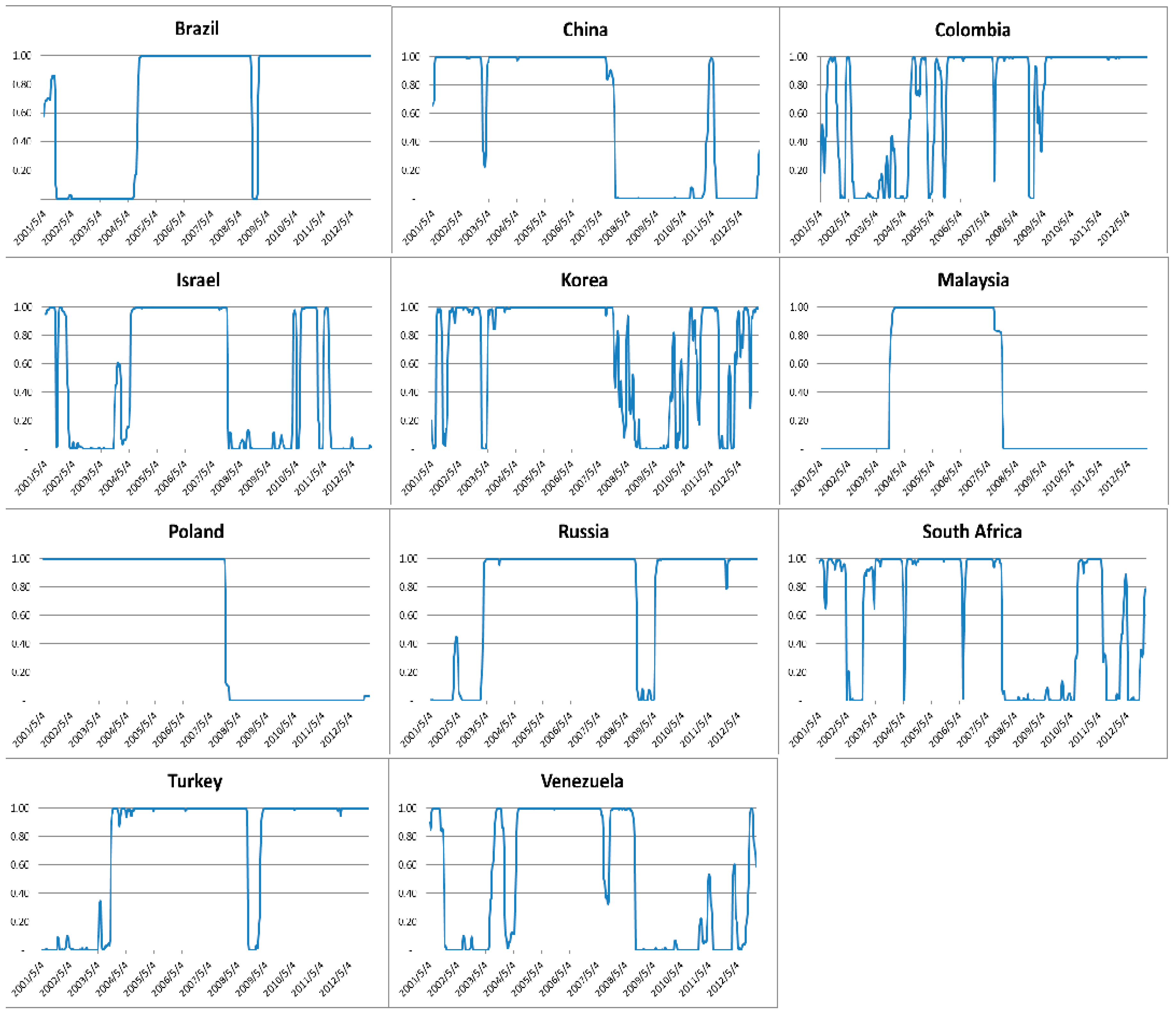
Figure 1 plots the smoothed probability of Regime 1, the good state, P[St = 1], fitted to the 11 countries’ CDS spread changes for the Regime Switching Model specification (b) which is specified in Equation (12). The values of the smoothed probability series are typically very close to either zero (Regime 2, bad state) or one (Regime 1, good state) and the smoothed probability series do not frequently switch between the good state and the bad state. The smoothed probability is of interest in economically interpreting the regime switching behavior of the CDS spread changes and determines if and when regime switches occur. During the 2008–2009 financial crisis, all the 11 countries entered regime 2 (bad state) for a certain period of time and then exit the bad state during the 2010–2011 recovery period. During the 2003–2007 economic expansion all countries were in the good state.

6. Cross Sectional Analysis

From the empirical analysis in the previous section we see that all the explanatory variables have an impact on the SCDS spread changes where local and regional variables show more influence in the good state and global variables have more influence in the bad state. We also witness a significant difference among the countries in terms of the extent of which these explanatory variables are associated with a country’s SCDS spread change. What are the determinants of these cross-sectional differences? The answer to this research question will be useful for emerging market investors in formulating sovereign credit risk management strategy that is specific to the characteristics of each emerging market country. First of all, we expect the more open an economy and the more it is integrated to the global economy, the stronger will be the influence of regional and global factors on its SCDS spread change. Second, there is likely to be a size effect, the smaller the economy, the more vulnerable it is to the regional and global shocks. Thus, both regional and global factors may play a more important role in affecting smaller country’s SCDS spread changes. Finally, there may be a regional effect. For example, due to their geographical and/or cultural characteristics, Asian countries may behave differently from European countries in terms of the determinants of their sovereign credit risks.

In conducting our cross-sectional analysis, we classify our countries into different subgroups independently based on four country-specific indicators representing openness/global integration (Kaopen Index; trade-to-GDP ratio; foreign direct investment (FDI) to GDP ratio) and the size of the economy (as proxied by GDP). We then examine and compare the sensitivities of SCDS spread change to the representative explanatory variables across the subgroups.

Table 8. Average values of indicators for each country.

Country	Kaopen Index	Import + Export (% of GDP)	FDI, Net Inflows (% of GDP)	GDP (MM)
Brazil	0.03	20.56	2.71	1,320,903.88
China	−1.17	67.82	3.67	2,753,506.67
Colombia	−0.29	29.20	3.56	200,148.08
Israel	2.13	55.35	3.83	175,681.59
Korea	0.13	74.00	0.49	862,100.87
Malaysia	−0.19	162.42	3.01	183,676.38
Poland	−0.05	64.96	3.46	364,760.02
Russia	−0.13	45.62	2.69	1,085,489.40
South Africa	−1.17	41.90	1.82	261,131.15
Turkey	−0.72	47.65	1.81	535,179.14
Venezuela	−0.62	25.75	1.05	202,169.33

Notes: This table summarizes average values of four market and economic indicators of the 11 countries being studied during the period of 2001 to 2012.

summarizes the average values of four market and economic indicators of the 11 countries during period of 2001 to 2012. From Table 8, we observe significant cross-sectional variations of country characteristics as captured by these indicators. For example, the trade-to-GDP ratio of Malaysia is almost eight times that of Brazil; whereas the FDI ratio of Israel is again almost eight times that of Korea.

To examine how these country-specific factors is related to the influence of different variables on SCDS, we divide the countries into two subgroups. The first subgroup of each indicator consists of six countries with lower values of the indicator and the second subgroup consists of the remaining five countries with higher values of the indicator.

Table 9. Sub-grouping of Countries.

	Kaopen	Import + Export (% of GDP)	FDI, Net Inflows (% of GDP)	GDP Size
subgroup of lower indicator value	China	Brazil	Korea	Israel
	South Africa	Venezuela	Venezuela	Malaysia
	Turkey	Colombia	Turkey	Colombia
	Venezuela	South Africa	South Africa	Venezuela
	Colombia	Russia	Russia	South Africa
	Malaysia	Turkey	Brazil	Poland
subgroup of higher indicator value	Russia	Israel	Malaysia	Turkey
	Poland	Poland	Poland	Korea
	Brazil	China	Colombia	Russia
	Korea	Korea	China	Brazil
	Israel	Malaysia	Israel	China

Notes: This table shows the sub-grouping of countries for each indicator. We divide the countries into two subgroups for the four indicators. The first subgroup consists of six countries with lower value of the indicator and the second subgroup consists of the remaining five countries with higher value of the respective indicator.

shows the sub-grouping of countries for each indicator.

As outlined in the previous sections, Equation (12) is our most comprehensive regime switching model that incorporates all local, regional and global factors. Based on regression results of Equation (12) as shown in Table 7, we select the four most significant explanatory variables to conduct the cross-sectional analysis. The four variables are $Re{s}_{R_{local}}$, $\Delta Rating,$ $Re{s}_{\Delta CD{S}_{Regional}}$ and $R_{S\&P}$.

Table 10. Cross sectional analysis of selected explanatory variables.

	Indicator	Subgroup	$\mathit{R}\mathit{e}{\mathit{s}}_{{\mathit{R}}_{\mathit{l}\mathit{o}\mathit{c}\mathit{a}\mathit{l}}}$		$\Delta \mathit{R}\mathit{a}\mathit{t}\mathit{i}\mathit{n}\mathit{g}$		$\mathit{R}\mathit{e}{\mathit{s}}_{\Delta \mathit{C}\mathit{D}{\mathit{S}}_{\mathit{R}\mathit{e}\mathit{g}\mathit{i}\mathit{o}\mathit{n}\mathit{a}\mathit{l}}}$		${\mathit{R}}_{\mathit{S}\&\mathit{P}}$
			S1	S2	S1	S2	S1	S2	S1	S2
Openness/	kaopen	Closed	−1.364 **	−3.445 *	−13.802	−23.029	2.683 **	0.461	−2.542 **	−1.65 **
Global Integration		Open	−1.515 **	1.324	−4.274 *	17.760	2.026 *	1.596 *	−1.715 **	−2.014 **
	Import + Export (% of GDP)	Closed	−0.913 **	−3.070 *	−10.977 *	−11.021	1.996 **	−0.030	−3.713 **	−1.492 **
		Open	−2.056 *	0.874 *	−7.663 *	3.351	2.851 **	2.184 *	−0.31 *	−2.203 **
	FDI, net inflows (% of GDP)	Closed	−0.861 **	−2.920 *	−11.648 *	−5.055	1.092 **	0.166	−3.393 **	−1.208 **
		Open	−2.118 *	0.693 *	−6.858 *	−3.809	3.935 **	1.949 *	−0.694 *	−2.543 **
Size	GDP size	Small	−1.304 **	−1.224 *	−5.776 *	−1.910	3.162 **	2.214 *	−1.702 **	−5.679 **
		Big	−1.587 **	−1.341 *	−13.904 *	−7.583	1.451 *	−0.507	−2.723 **	2.821 **

Notes: This table shows the average of the coefficients of the selected four explanatory variables (obtained from running our regime-switching model of Equation (12)) of the countries within each subgroup. The columns labelled by S1 (S2) consist of results for the good (bad) state.

shows the average of the coefficients of these four variables (obtained from running our regime-switching model of Equation (12)) of the countries within each subgroup. The columns labelled by S1 (S2) consist of results for the good (bad) state. For example, the average coefficient of $\mathrm{Res}\_{\mathrm{R}}_{\mathrm{local}}$ for the closed group for Kaopen in the good state (S1) is denoted as −1.364 **. The closed group for Kaopen has six countries namely China, South Africa, Turkey, Venezuela, Colombia and Malaysia and their coefficients of $Res\_R_{local}$ in the good state (S1) are respectively, −4.452 *, −0.629 ***, −1.054 ***, −1.057 ***, −0.809 *** and −0.186 * as shown in Table 7. The average in value therefore equals to −1.364 and the average in statistical significance is at 5% level (i.e., **). Below is a summary of the main findings from examining the average variations of the average coefficients of these four variables across subgroups of each indicator.

$Re{s}_{\Delta CD{S}_{Regional}}$: This factor, in general, has larger impact on open countries than closed countries for the openness indicator subgroups. This is especially true in the bad state (S2), consistent with the expectation that the open countries are more integrated with the regional economies while the contagion effect being more salient in the bad state. Comparing the two size indicator subgroups, $Re{s}_{\Delta CD{S}_{Regional}}$ has larger impact on small countries both in good and bad states. This is expected because, the smaller the economy, the easier it could be influenced by the surrounding economies. Especially in a global crisis, smaller countries with less diversified economies would be more affected because economic links are more important for such countries than larger countries. Larger countries are expected to be less affected by the surrounding economies than by its own local factors. Besides, larger countries tend to have more diverse economic composition and thus less susceptible to industry-specific shocks that propagate across borders.

$\Delta Rating$: Rating change has stronger impact in the good state than in the bad state for all indicator subgroups. This is consistent with our expectation that fundamental factors as captured by rating plays a stronger role in the good state, whereas its effect is weakened in the bad state as other financial factors dominate. The influence of rating is also more significant for closed than for open countries, suggesting fundamental factors are more influential in dictating the sovereign risk of closed countries.

$Re{s}_{R_{local}}$ and $R_{S\&P}$: For open countries, in the bad state, their SCDS spreads are more affected by ${\mathrm{R}}_{\mathrm{S}\&\mathrm{P}}$; whereas in the good state, they are more affected by $Re{s}_{R_{local}}$. This asymmetry reflects the market sentimental effect of flight-to-quality that only manifests itself in the bad state. For closed countries, their SCDS spreads are more affected by $Re{s}_{R_{local}}$ in the bad state, while $R_{S\&P}$ plays a stronger role in the good state. Finally, we find that $R_{S\&P}$ has the strongest influence for small countries in the bad state. This could be attributed to the fact that economic links are more important for smaller countries than larger countries with diverse economies. The strong effect of $R_{S\&P}$ in the good state suggests that the S&P 500 return captures fundamental global improvement that even benefits closed economies.

7. Conclusions

The weekly change of emerging market sovereign CDS spreads is affected by many market and economic variables. This paper examines the effect of a broad range of such variables including local financial, fundamental and global financial variables. The objective of the paper is to find the varying behavior of these variables on emerging market sovereign CDS in a two-state Markov regime switching environment.

We find that local, regional and fundamental variables such as local stock index return, exchange rate change, regional SCDS spread and credit rating change of the country influence the SCDS change more when the market is in a good state. Whereas global variables, such as US stock index return, have in general stronger influence in a bad state. Especially, when the regime is in a bad state, the single factor of US stock market return dominates other factors and its significance is much larger in the bad state than it is in the good state. This is consistent with the risk aversion and flight-to-quality assets behavior of investors when global market becomes volatile.

We also conduct cross sectional analysis to examine the behavior of the same explanatory variable on countries of different macroeconomic characters and reveal valuable findings. First, we find that more open countries are more integrated with the regional economies with the contagion effect being more salient in the bad state. Second, smaller countries with less diversified economies would be more affected a global crisis because economic links are more important for such countries than larger countries. Third, the influence of rating is more significant for closed than for open countries indicating that fundamental factors are more influential in dictating the sovereign risk of closed countries. Finally, we find that the market sentimental effect of flight-to-quality magnifies in the bad state and that $R_{S\&P}$ has the strongest influence for small countries in the bad state which could be attributed to the fact that economic links are more important for smaller countries than larger countries with diverse economies.

Our work opens a new page for studies on how CDS spreads vary with regimes and how various factors play their roles. Further research can certainly be done to improve the results in this paper as well as to expand the discussions in this paper.