Generalized Correlation Measures of Causality and Forecasts of the VIX Using Non-Linear Models

Abstract

This paper features an analysis of causal relations between the daily VIX, S&P500 and the daily realised volatility (RV) of the S&P500 sampled at 5 min intervals, plus the application of an Artificial Neural Network (ANN) model to forecast the future daily value of the VIX. Causal relations are analysed using the recently developed concept of general correlation Zheng et al. and Vinod. The neural network analysis is performed using the Group Method of Data Handling (GMDH) approach. The results suggest that causality runs from lagged daily RV and lagged continuously compounded daily return on the S&P500 index to the VIX. Sample tests suggest that an ANN model can successfully predict the daily VIX using lagged daily RV and lagged daily S&P500 Index continuously compounded returns as inputs.

1. Introduction

This paper features an analysis of the causal relationships between the daily value of the VIX and the volatility of the S&P500, as revealed by estimates of the realised volatility (RV) of the S&P500 index, sampled at 5 min intervals, to produce daily values, as calculated by the Oxford Man Institute of Quantitative Finance, utilising Reuter’s high frequency market data and provided in their ‘Realised Library.’ The causal analysis features an application of generalised measures of correlation, as developed by Zheng et al. [1] and Vinod [2]. This metric permits a more refined measure of causal direction.

The concept of causality has been a central philosophical issue for millennia. Aristotle in ‘Physics II 3 and Metaphysics V 2’ offered a general account of his concept of the four causes. (See http://classics.mit.edu/Aristotle/physics.2.ii.html). His account was general in the sense that it applied to everything that required an explanation, including artistic production and human action. He mentioned the: material cause: that out of which it is made, the efficient cause: the source of the objects principle of change or stability, the formal cause: the essence of the object. And the final cause: the end/goal of the object, or what the object is good for.

This treatment is far more encompassing than the customary treatment of causality in economics and finance. The modern treatment has been reduced to an analysis of correlation and statistical modelling. The origins of which can be traced back to the Scottish Enlightenment philosopher and historian, David Hume, who explored the relationship of cause and effect. Hume is recognised as a thorough going exponent of philosophical naturalism and as a precursor of contemporary cognitive science. Hume showed us that experience does not tell us much. Of two events, A and B, we say that A causes B when the two always occur together, that is, are constantly conjoined. Whenever we find A, we also find B and we have a certainty that this conjunction will continue to happen. This leads on to the concept of induction and a weak notion of necessity. (See: https://people.rit.edu/wlrgsh/HumeTreatise.pdf). It provides a backdrop to contemporary treatments of causality and statistical measures of association. The intricacies and difficulties involved in the concept of causality are further explored by Pearl [3].

In terms of statistical measures of association, or ‘constant contiguity,’ to adopt Hume’s term, Carl Pearson developed the correlation coefficient in the 1890s [4]. Granger [5], introduced the time series linear concept of ‘Granger’ causality. Zheng et al. [1] point out that one of the limitations of the correlation coefficient is that it does not account for asymmetry in explained variance. They developed broader applicable correlation measures and proposed a pair of generalized measures of correlation (GMC) which deal with asymmetries in explained variances and linear or nonlinear relations between random variables. Vinod [2] has further applied these measures to applied economics issues and developed an R library package, ‘generalCorr,’ for the application of these metrics, used in the analysis in this paper.

In this paper, we explore the directional causality between the VIX and RV estimates of the S&P500 volatility applying non-linear (GMC) methods and then engage in a further non-linear volatility forecasting exercise using Artificial Neural Network (ANN) methods. We do this using the GMDH shell program (http:www.gmdhshell.com). This program is built around an approximation called the Group Method of Data Handling. This approach is used in such fields as data mining, prediction, complex systems modelling, optimization and pattern recognition. The algorithms feature an inductive procedure that performs a sifting and ordering of gradually complicated polynomial models and the selection of the best solution by external criterion.

The paper is divided into five sections; Section 2, which follows this introduction, discusses the previous literature, whilst Section 3 introduces the data and research methods applied, Section 4 presents the results and section five concludes.

2. Prior Literature

In response to concerns that the original VIX calculation methodology had several weaknesses which made the issuance of VIX-related derivatives difficult, changes were made in 2003 by the CBOE. The calculation methodology was redefined to use the prices of synthetic 30-day options on the S&P500 index. See the discussions in Carr and Wu [6] and Whaley [7].

The VIX index is the “risk-neutral” expected stock market variance for the US S&P500 contract and is computed from a panel of options prices. It is termed the ‘fear index’ (see Whaley [8]) and provides an indication of both stock market uncertainty and a variance risk premium, which is also the expected premium from selling stock market variance in a swap contract. The VIX is based on “model-free” implied variances which are computed from a collection of option prices without the use of a specific pricing model (see, for example, Carr and Madan [9]).

There are various approaches to empirical work on the VIX. Baba and Sekura [10] investigate the role of US macroeconomic variables as leading indicators of regime shifts in the VIX index using a regime-switching approach. They suggest there are three distinct regimes in the VIX index during the 1990 to 2010 period corresponding to: a tranquil regime with low volatility, a turmoil regime with high volatility and a crisis regime with extremely high volatility. Fernandes et al. [11] undertake an analysis of the relationship between the VIX index and financial and macroeconomic factors.

There has been a great deal of work on derivatives related to the VIX. This is not the concern of this paper but the relevant ground is covered in Alexander et al. [12]. The fact that the VIX provides an estimate of the variance risk premium has been used to explore its relationship with stock market returns. See, for example, Bollerslev et al. [13] and Baekart and Horova [14], who take a similar approach.

The variance premium is defined by Bollerslev at al. [13], as the difference between the VIX, an ex-ante risk-neutral expectation of the future return variation over the $\left[t, t+1\right]$ time interval $\left(I{V}_t\right)$ and the ex post realized return variation over the $\left[t-1, t\right]$ time interval obtained from $R{V}_t$ measures:

$$VarianceRiskPremiu{m}_t=VR{P}_t\equiv ImpliedVolatilit{y}_t-RealisedVolatilit{y}_t$$

(1)

Bollerslev et al. [13] use the difference between implied and realized variation, or the variance risk premium, to explain a nontrivial fraction of the time-series variation in post-1990 aggregate stock market returns, with high (low) premia predicting high (low) future returns. The direction of the presumed causality is motivated from the implications from a stylized self-contained general equilibrium model incorporating the effects of time-varying economic uncertainty.

The current paper is concerned with the relationship between the VIX, implied volatility and S&P500 index continuously compounded returns but the focus is on an investigation of the causal path. It seeks to explore whether there is a stronger causal link between the VIX, to RV and stock returns, or in the reverse direction, from RV and stock returns to the VIX. The GMC analysis used in the paper suggests that the latter is the stronger causal path.

3. Data and Research Methods

3.1. Data Sample

We analyse the relationship between the VIX, the S&P500 Index and the realised volatility of the S&P500 index sampled at 5 min intervals, using daily data from 3 January 2000 to 12 December 2017, a total, after data cleaning and synchronization, of 4504 observations. The data for the VIX and S&P500 are obtained from Yahoo finance, whilst the realised volatility estimates are from the Oxford Man Realised Library (see: https://realized.oxford-man.ox.ac.uk).

In this paper, unlike the literature that uses the variance risk premium to forecast returns, we reverse the assumed direction of causality, based on our GMC analysis and predict the VIX on the basis of market returns and realised volatility.

The approach taken by Bollerslev et al. [13] and Baekart and Horova [14], is constructed on theoretical grounds and is not subjected to any tests of causal direction. A key feature of the current paper is to test, in practice, whether the causal direction runs from the VIX to returns on the S&P500 and estimates of daily RV, or, as we will subsequently demonstrate, in the reverse direction.

Given that we will be using regression analysis we require that our data sets are stationary. We know that price levels are non-stationary and so we use the continuously compounded returns on the S&P500 index. The results of Augmented Dickey Fuller tests shown in

Table 1. Tests of Stationarity: VIX and RV5MIN.

	ADF Test with Constant	Probability	ADF Test with Constant and Trend	Probability
VIX	−3.86664	0.002306 *	−4.11796	0.005859 *
RV5MIN	−7.70084	0.000 *	−7.80963	0.0000 *

Note: * Indicates significant at 0.01 level.

, strongly reject the null of non-stationarity for both the VIX and RV5MIN series, so we can combine them with the continuously compounded returns for the S&P500 Index in regression analysis, without the worry of estimating spurious regression.

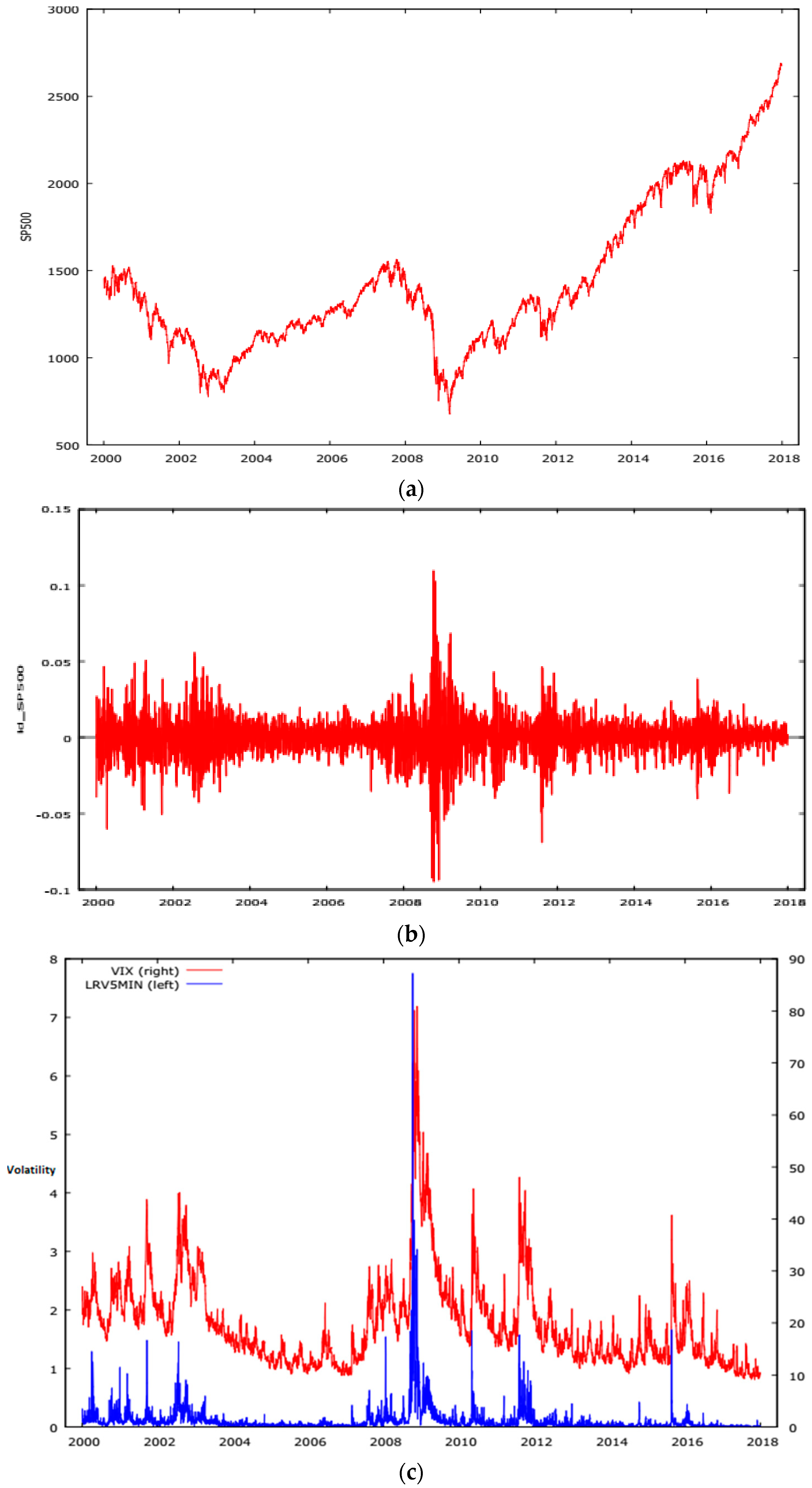
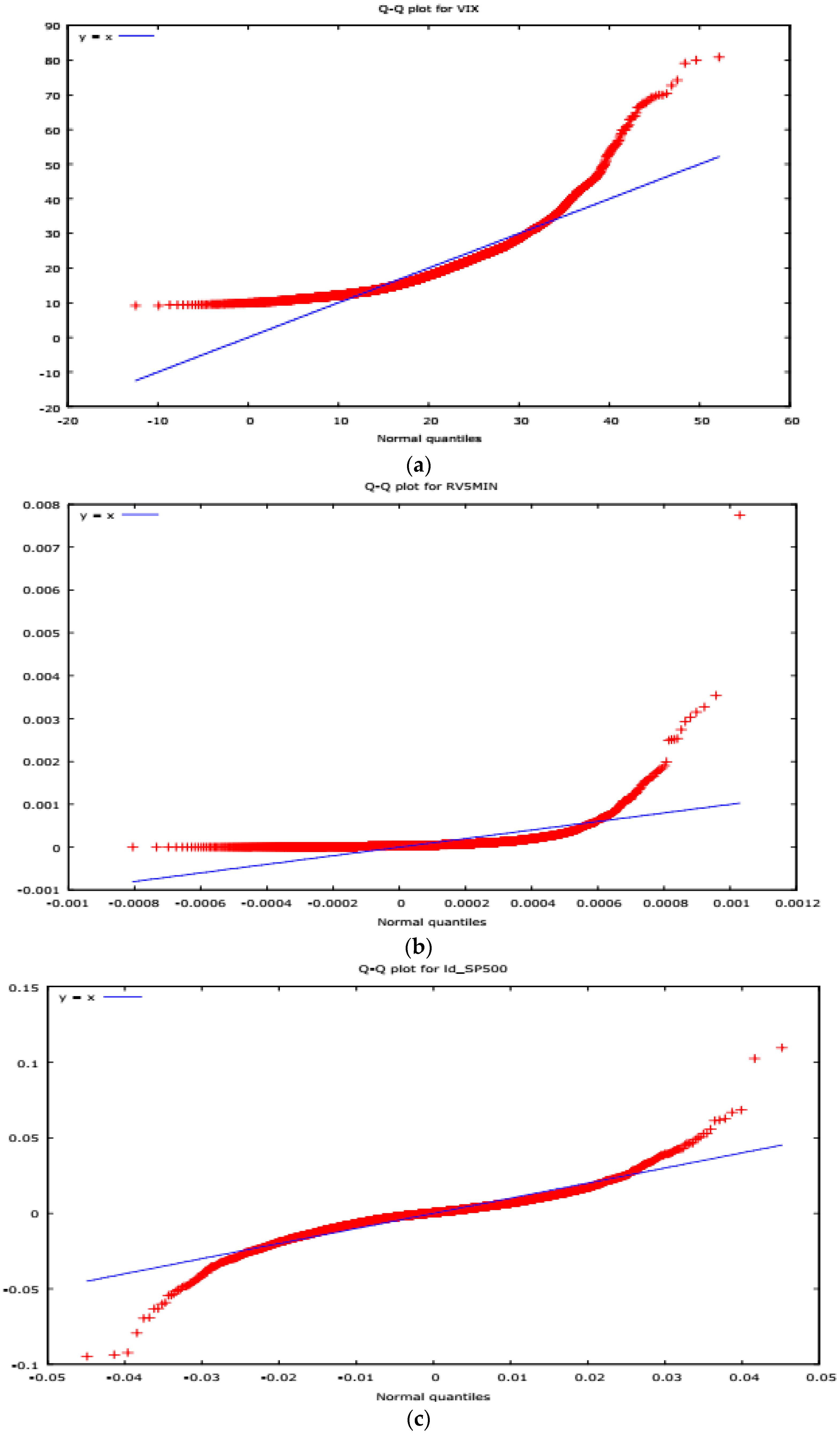
Plots of basic series are shown in Figure 1. Figure 2 shows quantile plots of our base series. All series show strong departures from a normal distribution in both tails of their distributions. These departures from Gaussian distributions are confirmed by the summary descriptions of the series provided in

Table 2. Data Series: Summary Statistics 3 January 2000 to 29 December 2017.

	VIX	S&P500 Return	RV5MIN
Mean	19.8483	0.000135262	0.111837
Median	17.6700	0.000522156	0.0501000
Minimum	9.14000	−0.0946951	0.000878341
Maximum	80.8600	0.109572	7.74774
Standard Deviation	8.75231	0.0121920	0.248439
Coefficient of Variation	0.440961	90.1361	2.22143
Skewness	2.09648	−0.203423	11.4530
Excess Kurtosis	6.94902	8.65908	242.166

. The summary statistics for our data sets in Table 2 confirm the results of the QQPlots and show that we have excess kurtosis in all three series and pronounced skewness in RV5MIN. We also undertook some preliminary regression and quantile regression analysis of the relationships between our three-base series to explore whether or not the relationship between the three series is linear.

3.2. Preliminary Regression Analysis

We estimated an OLS regression of the VIX regressed on the continuously compounded S&P500 return ’SPRET. The results are shown in

Table 3. OLS Regression of VIX on SPRET.

	Coefficient	t-Ratio	Probability Value
Constant	19.8485	43.35	0.00 ***
SPRET	−9.01551	−0.5215	0.6021
Adjusted R-squared
F(1, 4495)	0.271949		p-value (F) 0.602053
Ramsey Reset Test
Constant	−147551	−1.924	0.0544 *
SPRET	109932	2.105	0.0354 **
yhat^2	509.402	1.745	0.0811 *
yhat^3	−6.79270	−1.385	0.1662

Note: ***, **, * denotes significance at 1%, 5% and 10%.

. The slope coefficient is insignificant and the R squared is a miniscule 0.000158. The Ramsey Reset test suggests that the relationship is non-linear and that the regression is miss-specified.

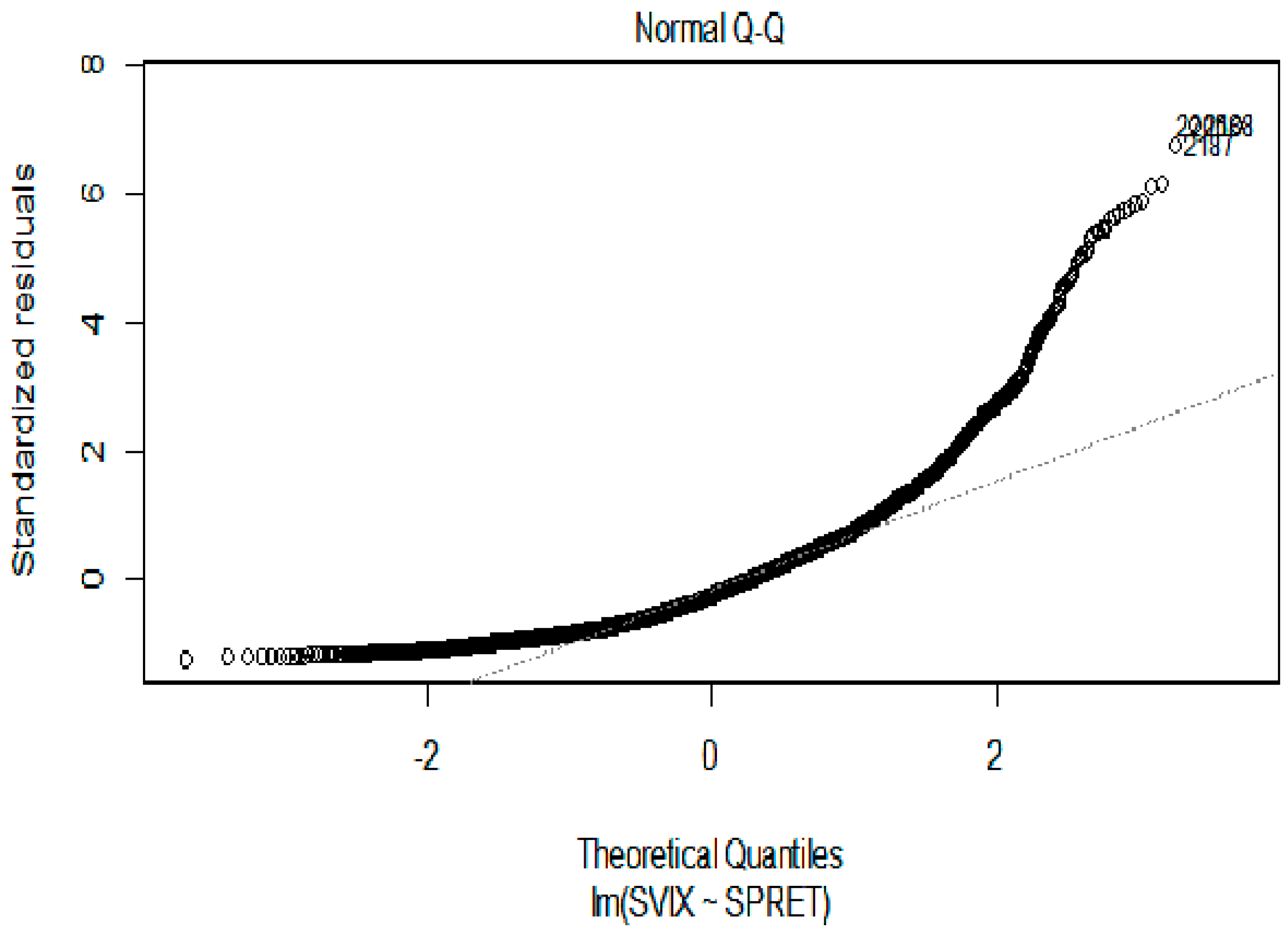
A QQplot of the residuals from this regression shown in Figure 3 also suggests that a linear specification is inappropriate.

To further explore the relationship between the sample variables we employed quantile regression analysis. Quantile Regression is modelled as an extension of classical OLS (Koenker and Bassett, [15]), in quantile regression the estimation of conditional mean as estimated by OLS is extended to similar estimation of an ensemble of models of various conditional quantile functions for a data distribution. In this fashion quantile regression can better quantify the conditional distribution of $(Y|X)$. The central special case is the median regression estimator that minimizes a sum of absolute errors. We get the estimates of remaining conditional quantile functions by minimizing an asymmetrically weighted sum of absolute errors, here weights are the function of the quantile of interest. This makes quantile regression a robust technique even in presence of outliers. Taken together the ensemble of estimated conditional quantile functions of $(Y|X)$ offers a much more complete view of the effect of covariates on the location, scale and shape of the distribution of the response variable.

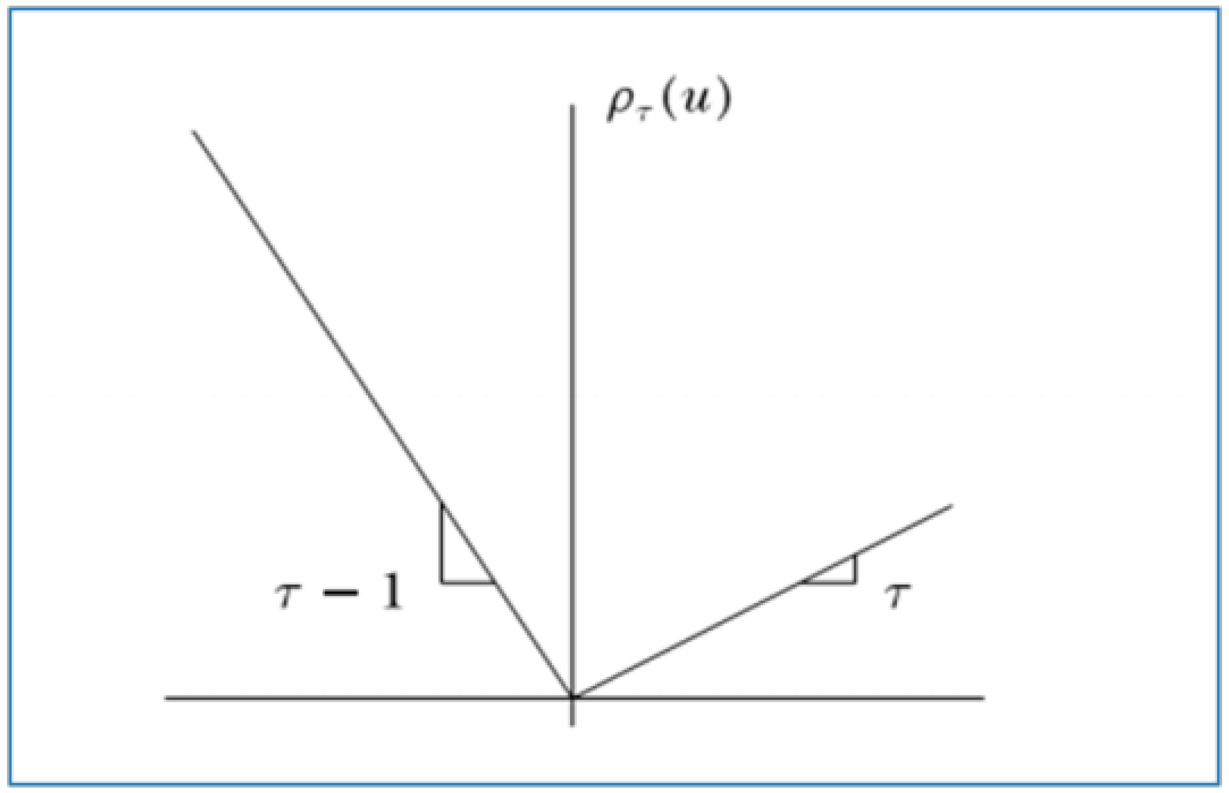
For parameter estimation in quantile regression, quantiles as proposed by Koenker and Bassett [15] can be defined through an optimization problem. To solve an OLS regression problem a sample mean is defined as the solution of the problem of minimising the sum of squared residuals, in the same way the median quantile (0.5%) in quantile regression is defined through the problem of minimising the sum of absolute residuals. The symmetrical piecewise linear absolute value function assures the same number of observations above and below the median of the distribution. The other quantile values can be obtained by minimizing a sum of asymmetrically weighted absolute residuals, (giving different weights to positive and negative residuals). Solving:

$$min\xi \epsilon R\sum {\rho }_{\tau }\left(y_i-\xi \right)$$

(2)

where ${\rho }_{\tau }(·)$ is the tilted absolute value function as shown in Figure 4, which gives the $\tau \mathrm{th}$ sample quantile with its solution. Taking the directional derivatives of the objective function with respect to $\xi$ (from left to right) shows that this problem yields the sample quantile as its solution.

After defining the unconditional quantiles as an optimization problem, it is easy to define conditional quantiles similarly. Taking the least squares regression model as a base to proceed, for a random sample, $y_1,y_2,\dots ,y_n$, we solve:

$$mi{n}_{\mu \epsilon R}{\displaystyle \sum }_{i=1}^n{(y_i-\mu )}^2,$$

(3)

Which gives the sample mean, an estimate of the unconditional population mean, EY. Replacing the scalar $\mu$ by a parametric function $\mu \left(x,\beta \right)$ and then solving:

$$mi{n}_{\mu \epsilon R^p}{\displaystyle \sum }_{i=1}^n{(y_i-\mu \left(x_i,\beta \right))}^2$$

(4)

gives an estimate of the conditional expectation function E(Y|x).

Proceeding the same way for quantile regression, to obtain an estimate of the conditional median function, the scalar $\xi$ in the first equation is replaced by the parametric function $\xi \left(x_t,\beta \right)$ and ${\tau }_{}$ is set to 1/2. The estimates of the other conditional quantile functions are obtained by replacing absolute values by ${\rho }_{\tau }(·)$ and solving:

$$mi{n}_{\mu \epsilon R^p}\sum {\rho }_{\tau }\left(y_i-\xi \left(x_i,\beta \right)\right)$$

(5)

The resulting minimization problem, when $\xi \left(x,\beta \right)$ is formulated as a linear function of parameters and can be solved very efficiently by linear programming methods. Further insight into this robust regression technique can be obtained from Koenker and Bassett [15] and Koenker [16].

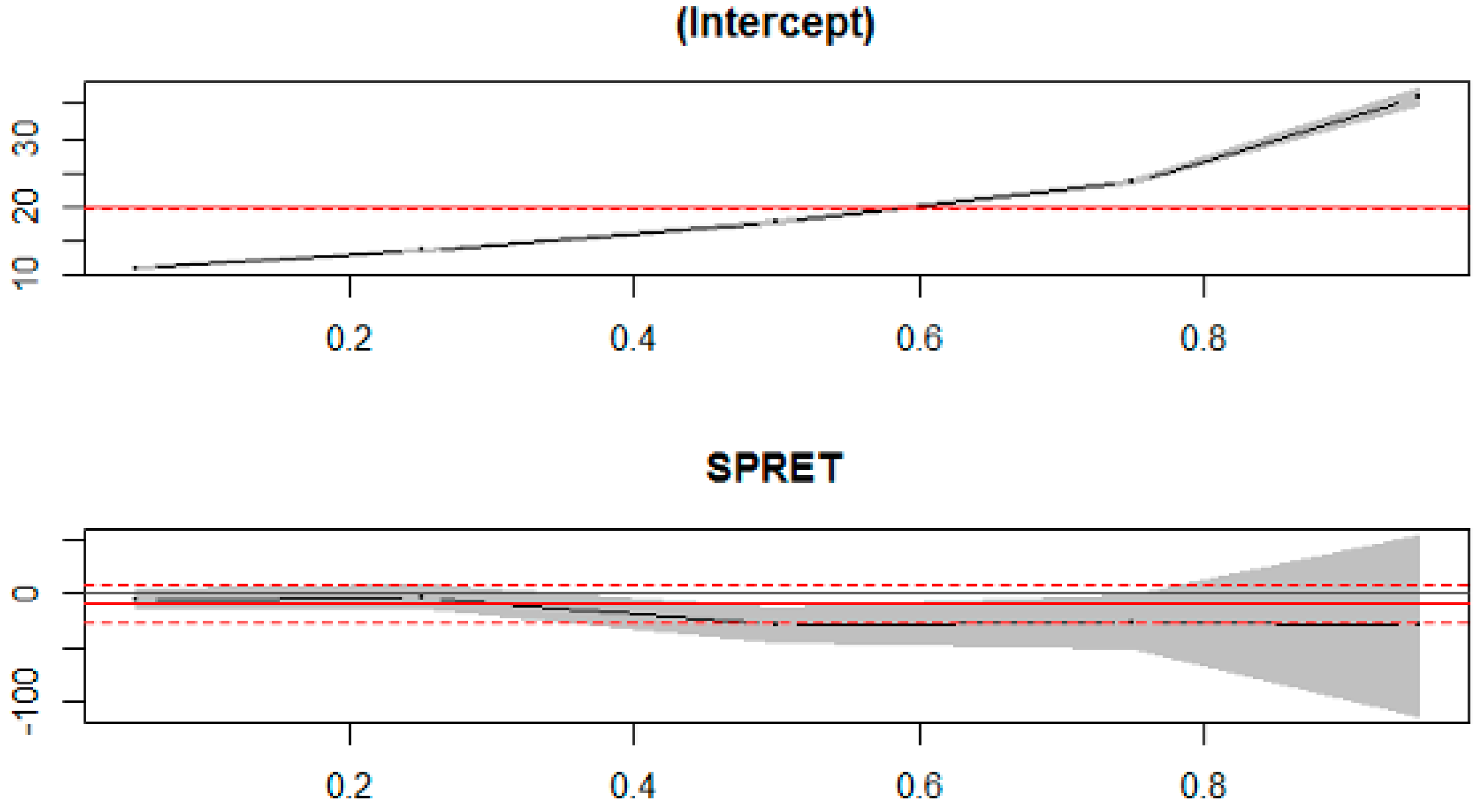
We used quantile regression to regress VIX on SPRET with the quantiles (tau), set at 0.05, 0.35, 0.5, 0.75 and 0.95 respectively. The results are shown in

Table 4. Quantile regression of VIX on SPRET (tau = 0.05, 0.25, 0.5, 0.75 and 0.95).

	Coefficient SPRET	t Value	Probability
tau = 0.05	−4.41832	−0.76987	0.44142
tau = 0.25	−2.79810	−0.43081	0.66663
tau = 0.50	−28.94626	−3.00561	0.00267 ***
tau = 0.75	−25.97296	−1.68811	0.09146 *
tau = 0.95	−29.40331	−0.57619	0.56452

Note: *** Significant at 1%, * Significant at 10%.

and Figure 5.

These preliminary regression results suggest a non-linear relationship between the VIX and SPRET. The existence of this non-linear relationship is consistent with findings by Busson and Vakil [17]. The importance of non-linearity will be explored further when we apply the metric provided by the Generalised Measure of Correlation which we introduce in the next subsection.

3.3. Econometric Methods

Zeng et al. [1] point out that despite its ubiquity there are inherent limitations in the Pearson correlation coefficient when it is used as a measure of dependency. One limitation is that it does not account for asymmetry in explained variances which are often innate among nonlinearly dependent random variables. As a result, measures dealing with asymmetries are needed. To meet this requirement, they developed Generalized Measures of Correlation (GMC). They commence with the familiar linear regression model and the partitioning of the variance into explained and unexplained portions

$$Var\left(X\right)=Var(E\left(X\mid Y\right)+E\left(Var\left(X\mid Y\right)\right),$$

(6)

Whenever $E\left(Y^2\right)<\infty$ and $E\left(X^2\right)<\infty$. Note that $E\left(Var\left(X\mid Y\right)\right)$ is the expected conditional variance of $X$ given $Y$ and therefore can be interpreted as the explained variance of $X$ by $Y.$ Thus, we can write:

$$\frac{E\left(Var\left(X\mid Y\right)\right)}{Var\left(X\right)}=1-\frac{E\left(Var\left(X\mid Y\right)\right)}{Var\left(X\right)}=1-\frac{E({\{X-E\left(X\mid Y\right)\}}^2}{Var\left(X\right)}.$$

The explained variance of $Y$ given $X$ can similarly be defined. This leads Zheng et al. [1] to define a pair of generalised measures of correlation (GMC) as:

$$\left\{GMC\left(Y\mid X\right),GMC\left(X\mid Y\right)\right\}=\{1-\frac{E({\{Y-E\left(Y\mid X\right)\}}^2}{Var\left(Y\right)},1-\frac{E({\{X-E\left(X\mid Y\right)\}}^2}{Var\left(X\right)}\}.$$

(7)

This pair of GMC measures has some attractive properties. It should be noted that the two measures are identical when $\left(X,Y\right)$ is a bivariate normal random vector.

Vinod [2] takes this measure in Expression (2) and reminds the reader that it can be viewed as kernel causality. The Naradaya Watson kernel regression is a non-parametric technique used in statistics to estimate the conditional expectation of a random variable. The objective is to find a non-linear relation between a pair of random variables X and Y. In any nonparametric regression, the conditional expectation of a variable Y relative to a variable X could be written $E\left(Y|X\right)=m\left(X\right)$ where $m$ is an unknown function.

Naradaya [18] and Watson [19] proposed estimating m as a locally weighted average employing a kernel as a regression function.

$$\widehat{m_h}\left(x\right)=\frac{{{\displaystyle \sum }}_{i=1}^n{K}_{h\left(x-x_i\right)y_i}}{{{\displaystyle \sum }}_{j=1}^n{K}_{h\left(x-x_j\right)}},$$

where $K$ is a kernel with bandwidth h. The denominator is a weighting term that sums to 1.

$GMC\left(Y\mid X\right)$ is the coefficient of determination $R^2$ of the Nadaraya-Watson nonparametric Kernel regression:

$$y=g\left(X\right)+ϵ=E\left(Y\mid X\right)+ϵ,$$

(8)

where $g\left(X\right)$ is a nonparametric, unspecified (nonlinear) function. Interchanging $X$ and $Y$, we obtain the other $GMC\left(X\mid Y\right)$ defined as the $R^2$ of the Kernel regression:

$$X=g^{\prime }\left(Y\right)+{ϵ}^{\prime }=E\left(XY\right)+{ϵ}^{\prime .}.$$

(9)

Vinod [2] defines $\delta =GMC\left(X\mid Y\right)-GMC\left(X\mid Y\right)$ as the difference of two population $R^2$ values. When $\delta <0$, we know that $X$ better predicts $Y$ than vice versa. Hence, we define that $X$ kernel causes $Y$ provided the true unknown $\delta <0$. Its estimate ${\delta }^{\prime }$ can be readily computed by means of regression.

Zheng et al. [1] demonstrate that GMC can lead to a more refined version of the concept of Granger-causality. They assume an order one bivariate linear autoregressive model. $Y_t$ Granger-causes $X_t$ if:

$$E[{\{X_t-E\left(X_t\mid X_{t-1}\right)\}}^2>E[{\{X_t-E\left(X_t\mid X_{t-1},Y_{t-1}\right)\}}^2,$$

(10)

Which suggests that $X_t$ can be better predicted using the histories of both $X_t$ and $Y_t$ than using the history of $X_t$ alone. Similarly, we would say $X_t$ Granger-causes $Y_t$ if:

$$E[{\{Y_t-E\left(Y_t\mid Y_{t-1}\right)\}}^2>E[{\{Y_t-E\left(Y_t\mid Yt-1,X_{t-1}\right)\}}^2.$$

(11)

They use the fact $E(Var\left(X_t\mid X_{t-1}\right)=E(\{X_t-E(X_t\mid X_{t-1}{\}}^2)$ and $E[{\{E\left(X_t\mid X_{t-1}\right)-E\left(X_t\mid X_{t-1},Y_{t-1}\right)\}}^2\left]=E\right[{\{X_t-E\left(X_t\mid X_{t-1}\right)\}}^2-E[{\{X_t-E\left(X_t\mid X_{t-1},Y_{t-1}\right)\}}^2].$ Which suggests that (5) is equivalent to:

$$1-\frac{E[{\{X_t-E\left(X_t\mid X_{t-1},Y_{t-1}\right)\}}^2}{E\left(Var\left(X_t\mid X_{t-1}\right)\right)}>0.$$

(12)

In the same way (6) is equivalent to:

$$1-\frac{E[{\{Y_t-E\left(Y_t\mid Y_{t-1},X_{t-1}\right)\}}^2}{E\left(Var\left(Y_t\mid Y_{t-1}\right)\right)}>0.$$

(13)

They add that when both (5) and (6) are true, there is a feedback system.

Suppose that $\left\{X_t,Y_t\right\},Y_t>0$ is a bivariate stationary time series. Zheng et al. [1] define Granger causality generalised measures of correlation as:

$$GcGMC=\left(X_t\mid {\mathcal{F}}_{t-1}\right)=1-\frac{E{[\{X_t-\mid X_{t-1},X_{t-1},\dots ,Y_{t-1},Y_{t-2},\dots ,)\}}^2]}{E\left(Var\left(X_t\mid X_{t-1},X_{t-2},\dots \right)\right)},$$

(14)

$$GcGMC=\left(Y_t\mid {\mathcal{F}}_{t-1}\right)=1-\frac{E{[\{Y_t-\mid Y_{t-1},Y_{t-1},\dots ,X_{t-1},X_{t-2},\dots ,)\}}^2]}{E\left(Var\left(Y_t\mid Y_{t-1},Y_{t-2},\dots \right)\right)}$$

(15)

where ${\mathcal{F}}_{t-1}=\sigma \left(X_{t-1},X_{t-2},\dots ,Y_{t-1},Y_{t-2},\dots \right).$

Zheng et al. [1] suggest that if:

• $GcGMC=\left(X_t\mid {\mathcal{F}}_{t-1}\right)>0,$ they say $Y$ Granger causes $X.$
• $GcGMC=\left(Y_t\mid {\mathcal{F}}_{t-1}\right)>0$, they say $X$ Granger causes $Y.$
• $GcGMC=\left(X_t\mid {\mathcal{F}}_{t-1}\right)>0$ and $GcGMC=\left(Y_t\mid {\mathcal{F}}_{t-1}\right)>0,$ they say they have a feedback system.
• $GcGMC=\left(X_t\mid {\mathcal{F}}_{t-1}\right)>GcGMC=\left(Y_t\mid {\mathcal{F}}_{t-1}\right),$ they say $X$ is more influential than $Y$
• $GcGMC=\left(Y_t\mid {\mathcal{F}}_{t-1}\right)>GcGMC=\left(X_t\mid {\mathcal{F}}_{t-1}\right),$ they say $Y$ is more influential than $X.$

We explore the relationship between the VIX, the lagged continuously compounded return on the S&P500 Index, (LSPRET) and the lagged daily realised volatility on the S&P500, sampled at 5 min intervals within the day (LRV5MIN). Once we have established causal directions between these variables, we use them to construct our ANN model. The ANN model is discussed in the next section.

3.4. Artificial Neural Net Models

There are a variety of approaches to neural net modelling. A simple neural network model with linear input, $D$ hidden units and activation function $g,$ can be written as:

$$x_{t+s}={\beta }_0+{\displaystyle \sum }_{j=1}^D{\beta }_{j}g({\gamma }_{0j}+{\displaystyle \sum }_{i=1}^m{\gamma }_{ij}{x}_{t-\left(i-1\right)d}).$$

(16)

However, we choose to apply a nonlinear neural net modelling approach, using the GMDH shell program (GMDH LLC 55 Broadway, 28th Floor New York, NY 10006) (http:www.gmdhshell.com). This program is built around an approximation called the ‘Group Method of Data Handling.’ This approach is used in such fields as data mining, prediction, complex systems modelling, optimization and pattern recognition. The algorithms feature an inductive procedure that performs a sifting and ordering of gradually complicated polynomial models and the selection of the best solution by external criterion.

A GMDH model with multiple inputs and one output is a subset of components of the base function:

$$Y\left(x{i}_1,\dots ,x_n\right)=a_0+{\displaystyle \sum }_{i=1}^m{a}_i{f}_i,$$

(17)

where $f$ are elementary functions dependent on different inputs, $a$ are unknown coefficients and $m$ is the number of base function components.

In general, the connection between input-output variables can be approximated by the Volterra functional series, the discrete analogue of which is the Kolmogorov-Gabor polynomial:

$$y=a_0+{\displaystyle \sum }_{i=1}^m{a}_i{x}_i+{\displaystyle \sum }_{i=1}^m{\displaystyle \sum }_{{}_{j=1}}^m{a}_{ij}{x}_i{x}_j+{\displaystyle \sum }_{i=1}^m{\displaystyle \sum }_{j=1}^m{\displaystyle \sum }_{k=1}^m{a}_{ijk}{x}_i{x}_j{x}_k+\dots ,$$

(18)

where, $x=\left(x_i,x_2,\dots ,x_m\right)$, the input variables vector and $A=\left(a_0,a_1,a_2,\dots ,a_m\right)$ the vector of weights. The Kolmogorov-Gabor polynomial can approximate any stationary random sequence of observations and can be computed by either adaptive methods or a system of Gaussian normal equations. Ivakhnenko [20] developed the algorithm, ‘The Group Method of Data Handling (GMDH)’ by using a heuristic and perceptron type of approach. He demonstrated that a second-order polynomial (Ivakhnenko polynomial: $y=a_0+a_1{x}_i+a_2{x}_j+a_3{x}_i{x}_j+a_4{x}_i^2+a_5{x}_j^2)$ can reconstruct the entire Kolmogorov-Gabor polynomial using an iterative perceptron-type procedure.

4. Results

4.1. GMC Analysis

Vinod’s (2017) R library package ‘generalCorr’ is used to assess the direction of the causal paths between the VIX and lagged values of the S&P500 continuously compounded return LSPRET and the lagged daily estimated realised volatility for the S&P500 index, LRV5MIN. The results of the analysis are shown in

Table 5. GMC analysis of the relationship between the VIX and LRV5MIN.

	VIX	LRV5MIN
VIX	1.000	0.7821467
LRV5MIN	0.608359	1.000
Test of the difference between the two paired correlations
t = 21.26	probability = 0.0

.

We use the R ‘generalCorr’ package to undertake the analysis shown in Table 5. The output matrix is seen to report the cause’ along columns and ‘response’ along the rows. The value of 0.7821467 in the R.H.S. of the second row of Table 5 is larger than the value 0.608359 in the second column, third row of Table 5. These are our two generalised measures of correlation, when we first condition the VIX on LRV5MIN, in the second row of Table 5 and LRV5MIN on the VIX in the third row of Table 5. This suggests that causality runs from LRV5MIN, the lagged daily value of the realised volatility of the S&P500 index, sample at 5 min intervals.

We also test the significance of the difference between these two generalised measures of correlation. Vinod suggests a heuristic test of the difference between two dependent correlation values. Vinod [2] suggests a test based on a suggestion by Fisher [21], of a variance stabilizing and normalizing transformation for the correlation coefficient, $r,$ defined by the formula: $r=tanh\left(z\right)$, involving a hyperbolic tangent:

$$z=ta{n}^{-1}r=\frac{1}{2}log\frac{1+r}{1-r}.$$

(19)

The application of the above test suggests a highly significant difference between the values of the two correlation statistics in Table 5.

We also analyse the relationship between the VIX and the lagged daily continuously compounded return on the S&P500 index, LSPRET. The results are shown in

Table 6. GMC analysis of the relationship between the VIX and LSPRET.

	VIX	LSPRET
VIX	1.000	0.5519368
LSPRET	0.153411	1.000
Test of the difference between the two paired correlations
t = 24.07	probability = 0.0

and suggest that lagged value of the daily continuously compounded return on the S&P500 index, LSPRET, drives the VIX. This is because the generalised correlation measure of the VIX conditioned on LSPRET is 0.5519368, whilst the generalised correlation measure of LSPRET conditioned on the VIX is only 0.153411. Once again, these two measures are significantly different.

Regression analysis suggested that the relationship was non-linear. We proceed to an ANN model which will be used for forecasting the VIX. Given that the GMC analysis suggests a stronger direction of correlation running from LRV5MIN and LSPRET to the VIX, rather than vice-versa, we use these two lagged daily variables as the predictor variables in our ANN modelling and forecasting.

4.2. ANN Model

Our neural network analysis is run on 80 per cent of the observations in our sample and then its out-of-sample forecasting performance is analysed on the remaining 20 per cent, of the total sample of 4504 observations. The idea of the GMDH-type algorithms used in the GMDH Shell program is to apply a generator using gradually more complicated models and select the set of models that show the highest forecasting accuracy when applied to a previously unseen data set, which in this case is the 20 per cent of the sample remaining, which is used as a validation set. The top-ranked model is claimed to be the optimally most-complex one.

GMDH-type neural networks which are also known as polynomial neural networks employ a combinatorial algorithm for the optimization of neuron connection. The algorithm iteratively creates layers of neurons with two or more inputs. The algorithm saves only a limited set of optimally-complex neurons that are denoted as the initial layer width. Every new layer is created using two or more neurons taken from any of the previous layers. Every neuron in the network applies a transfer function (usually with two variables) that allows an exhaustive combinatorial search to choose a transfer function that predicts outcomes on the testing data set most accurately. The transfer function usually has a quadratic or linear form but other forms can be specified. GMDH-type networks generate many layers but layer connections can be so sparse that their number may be as small as a few connections per layer.

Since every new layer can connect to previous layers the layer width grows constantly. If we take into account that only rarely the upper layers improve the population of models, we proceed by dividing the additional size of the next layer by two and generate only half of the neurons generated by the previous layer, that is, the number of neurons N at layer k is $N_K=0.5\times N_{k-1}$. This heuristic makes the algorithm quicker whilst the chance of reducing the model’s quality is low. The generation of new layers ceases when either a new layer does not show improved testing accuracy than previous layer, or in circumstances in which the error was reduced by less than 1%.

In the case of the model reported in this paper, we used a maximum of 33 layers and the initial layer width was a 1000, whilst the neuron function was given by $a+x_i+x_i{x}_j+x_i^2$. The ANN regression analysis produces a complex non-linear model which is shown in

Table 7. ANN regression model—dependent variable the VIX.

Y1 = −22.5101 + N107(1.01249) − $\mathit{N}{\mathbf{107}}^{{\mathbf{0.00364084}}^{\mathbf{2}}}$ + N87(1.67752) − $\mathit{N}{\mathbf{87}}^{{\mathbf{0.211077}}^{\mathbf{2}}}$

N87 = −8.10876 + $LSPRE{T}^{{1919.7}^2}$ + N99(1.66543) − $N{99}^{{0.0120732}^2}$

N99 = −18.9937 − LRV5MIN(669.032) + LRV5MIN(N100)(1297.44) − $LRV5MI{N}^{1.09098\mathrm{e}+{07}^2}$ + N100(2.8838) − $N{100}^{{0.0509041}^2}$

N100 = 18.6936 + LRV5MIN(48378) − $N{107}^{{0.00976245}^2}$

N107 = 17.0884 + LRV5MIN(20457.2) − LSPRET(50.0534) + $LSPRE{T}^{{3277.01}^2}$

.

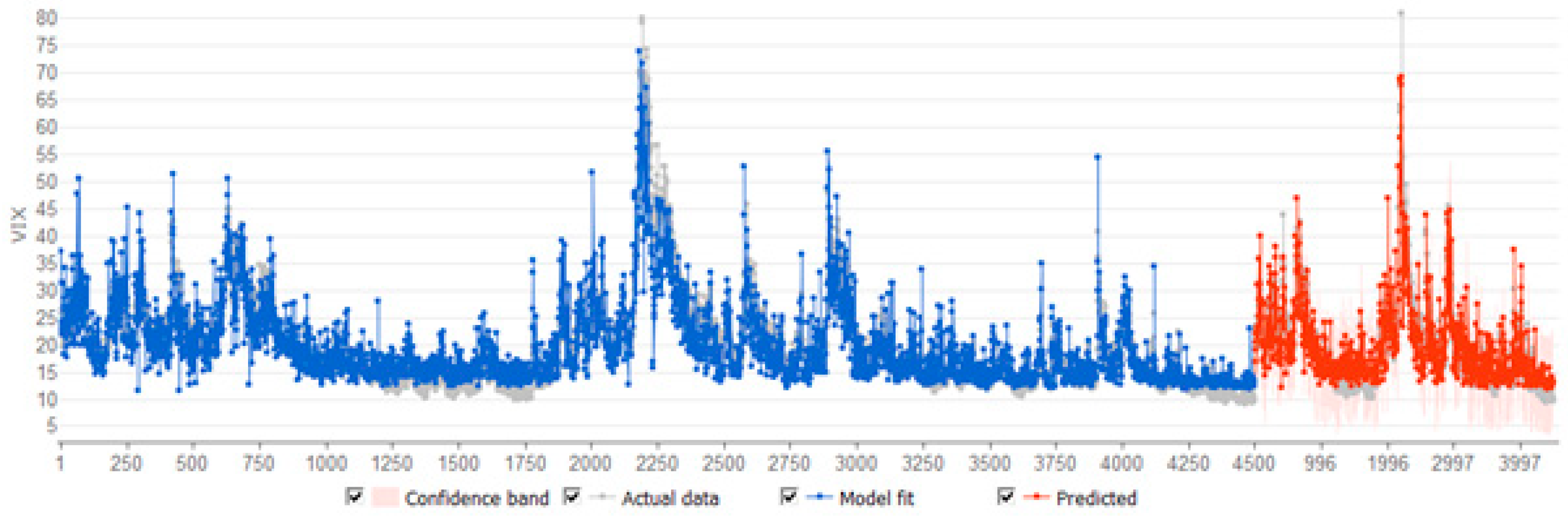
A plot of the ANN model fit is shown in Figure 6. The model appears to be a good fit, within the estimation period and in the 20 per cent of the sample used as a hold-out forecast period. This is confirmed by the diagnostics for the ANN model, reported in

Table 8. ANN regression model diagnostics.

	Model Fit	Predictions
Mean Absolute Error	3.16466	3.14658
Root Mean Square Error	4.47083	4.36716
Standard Deviation of Residuals	4.47083	4.36697
$\mathrm{Coefficient}\mathrm{of}\mathrm{Determination}{R}^2$	0.738519	0.752232

. The mean absolute error is smaller in the forecasts with a value of 3.14658, than it is when the model is being fitted, with a value of 3.16466. Similarly, the $R^2$ is higher in the forecast hold out sample, with a value of 75 percent, than in the model fitting stage, in which it has a value of almost 74 percent.

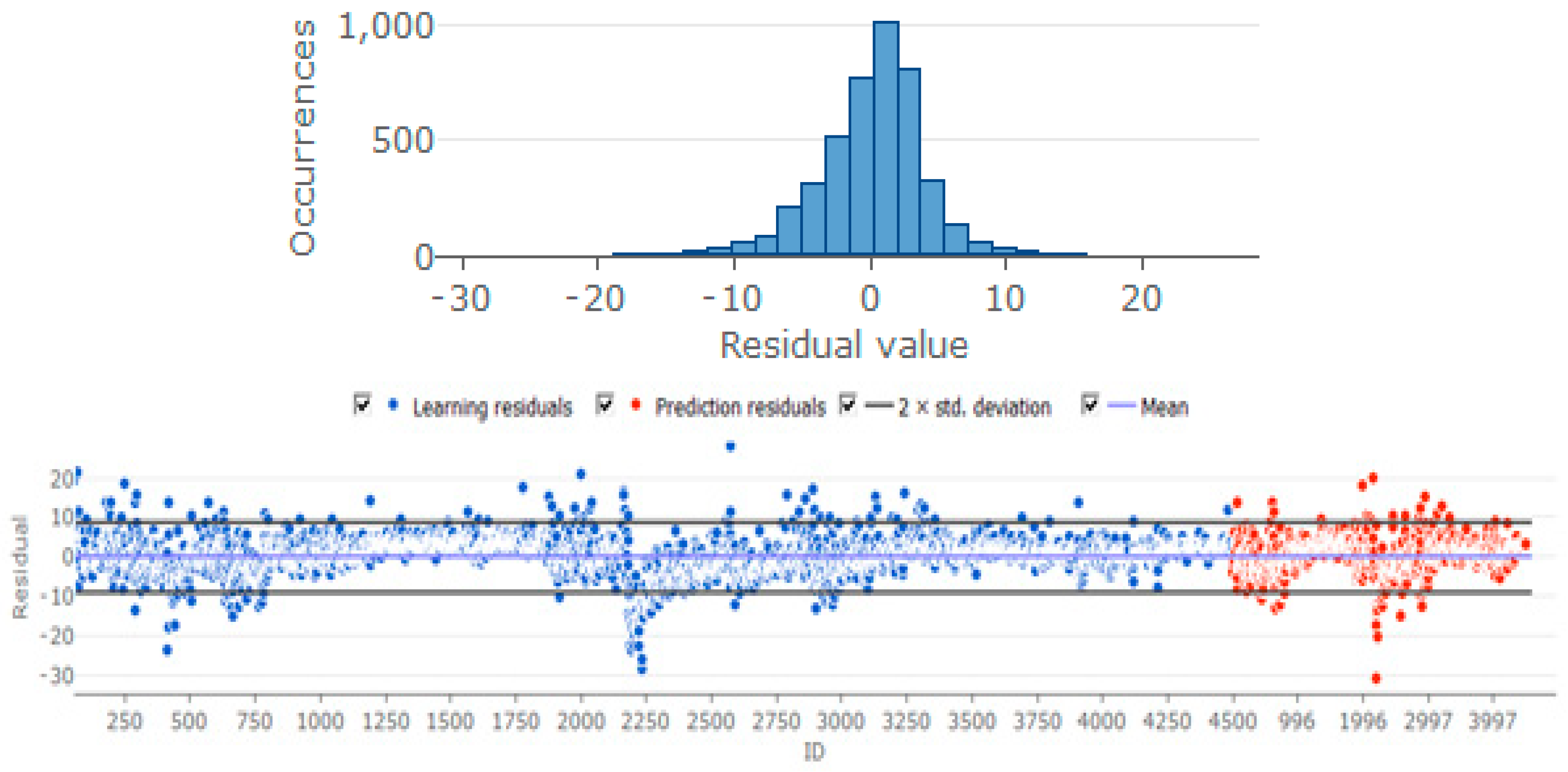
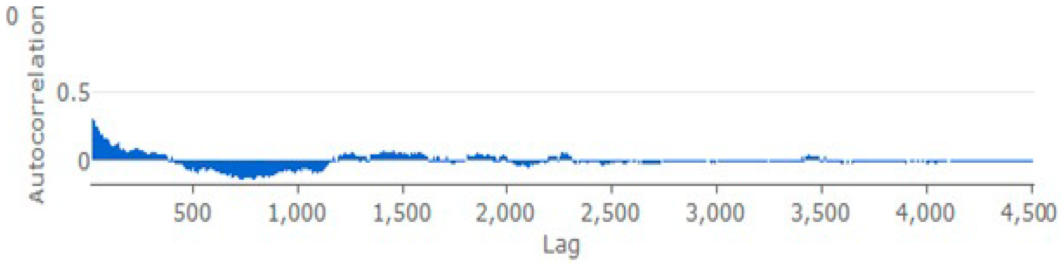
The diagnostic plots of the behaviour of the residuals, shown in Figure 7, also appears to show acceptable behaviour. Most of the residuals plot within the error bands, the residual histogram is approximately normal, though there is some evidence of persistence in the autocorrelations suggestive of ARCH effects.

As a further check on the mechanics of the model, we explored the effect on the root mean square errors in the forecasts if we replaced the two explanatory variable’s observations with their means successively. LRV5MIN has the largest effect with an impact on RMSE of 10.5364% whilst LSPRET had an impact of 4.57003%. This is consistent with the previous GMC results which suggested that LRV5MIN had a relatively higher GMC with the VIX.

5. Conclusions

The paper featured an analysis of causal relations between the VIX and lagged continuously compounded returns on the S&P500, plus lagged realised volatility (RV) of the S&P500 sampled at 5 min intervals. Causal relations were analysed using the recently developed concept of general correlation Zheng et al. [1] and Vinod [2]. The results strongly suggested that causal paths ran from lagged returns on the S&P500 and lagged RV on the S&P500 to the VIX. The GMC analysis suggested that correlations running in this direction were stronger than those in the reverse direction. Statistical tests suggested that the pairs of correlated correlations analysed were significantly different.

An ANN model was then developed, based on the causal paths suggested, using the Group Method of Data Handling (GMDH) approach. The complex non-linear model developed performed well in both in and out of sample tests. The results suggest an ANN model can be used successfully to predict the daily VIX using lagged daily RV and lagged daily S&P500 Index continuously compounded returns as inputs.

References

- Zheng, S.; Shi, N.-Z.; Zhang, Z. Generalized measures of correlation for asymmetry, nonlinearity, and beyond. J. Am. Stat. Assoc. 2012, 107, 1239–1252. [Google Scholar] [CrossRef]
- Vinod, H.D. Generalized correlation and kernel causality with applications in development economics. Commun. Stat. Simul. Comput. 2017, 46, 4513–4534. [Google Scholar] [CrossRef]
- Pearl, J. The foundations of causal inference. Sociol. Methodol. 2010, 40, 75149. [Google Scholar] [CrossRef]
- Pearson, K. Notes on regression and inheritance in the case of two parents. Proc. R. Soc. Lond. 1895, 58, 240–242. [Google Scholar] [CrossRef]
- Granger, C. Investigating causal relations by econometric methods and cross-spectral methods. Econometrica 1969, 34, 424–438. [Google Scholar] [CrossRef]
- Carr, P.; Wu, L. A tale of two indices. J. Deriv. 2006, 13, 13–29. [Google Scholar] [CrossRef]
- Whaley, R. Understanding the VIX. J. Portf. Manag. 2006, 35, 98–105. [Google Scholar] [CrossRef]
- Whaley, R.E. The investor fear gauge. J. Portf. Manag. 2000, 26, 12–17. [Google Scholar] [CrossRef]
- Carr, P.; Madan, D. Towards a theory of volatility trading. In Volatility: New Estimation Techniques for Pricing Derivatives; Jarrow, R., Ed.; Risk Books: London, UK, 1998; Chapter 29; pp. 417–427. [Google Scholar]
- Baba, N.; Sakurai, Y. Predicting regime switches in the VIX index with macroeconomic variables. Appl. Econ. Lett. 2011, 18, 1415–1419. [Google Scholar] [CrossRef]
- Fernandes, M.; Medeiros, M.C.; Scharth, M. Modeling and predicting the CBOE market volatility index. J. Bank. Financ. 2014, 40, 1–10. [Google Scholar] [CrossRef] [Green Version]
- Alexander, C.; Kapraun, J.; Korovilas, D. Trading and investing in volatility products. J. Int. Money Financ. 2015, 24, 313–347. [Google Scholar] [CrossRef]
- Bollerslev, T.; Tauchen, G.; Zhou, H. Expected stock returns and variance risk premia. Rev. Financ. Stud. 2009, 22, 44634492. [Google Scholar] [CrossRef]
- Bekaert, G.; Hoerova, M. The VIX, the variance premium and stock market volatility. J. Econ. 2014, 183, 181–192. [Google Scholar] [CrossRef] [Green Version]
- Koenker, R.W.; Bassett, G. Regression quantiles. Econometrica 1978, 46, 33–50. [Google Scholar] [CrossRef]
- Koenker, R. Quantile Regression; Cambridge University Press: Cambridge, UK, 2005. [Google Scholar]
- Buson, M.G.; Vakil, A.F. On the non-linear relationship between the VIX and realized SP500 volatility. Invest. Manag. Financ. Innov. 2017, 14, 200–206. [Google Scholar]
- Nadaraya, E.A. On estimating regression. Theory Probab. Appl. 1964, 9, 141–142. [Google Scholar] [CrossRef]
- Watson, G.S. Smooth regression analysis. Sankhyā Indian J. Stat. Ser. A 1964, 26, 359–372. [Google Scholar]
- Ivakhnenko, A.G. The group method of data handling—A rival of the method of stochastic approximation. Sov. Autom. Control 1968, 1, 43–55. [Google Scholar]
- Fisher, R.A. On the mathematical foundations of theoretical statistics. Philos. Trans. R. Soc. Lond. A 1922, 222, 309–368. [Google Scholar] [CrossRef]
Figure 1.
Plots of Base Series. (a) S&P500 INDEX; (b) S&P500 INDEX CONTINUOUSLY COMPOUNDED RETURNS; (c) VIX and RV5MIN.
Figure 2.
QQPlots of Base Series. (a) QQPLOT VIX; (b) QQPlot RV5MIN; (c) QQPLOT S&P500 RETURNS.
Figure 3.
QQplot of residuals from OLS regression of VIX on SPRET.
Figure 4.
Quantile regression function.
Figure 5.
Quantile regression of VIX on SPRET, estimates and error bands.
Figure 6.
ANN regression model fit.
Figure 7.
Residual diagnostic plots.