Financial Security and Optimal Scale of Foreign Exchange Reserve in China


1
School of Economics, Fudan University, Shanghai 200433, China
2
School of Finance, Shanghai University of Finance and Economics, Shanghai 200433, China
*
Author to whom correspondence should be addressed.
†
These authors contributed equally to this work.
Sustainability 2018, 10(6), 1724; https://doi.org/10.3390/su10061724
Submission received: 18 April 2018
/
Revised: 17 May 2018
/
Accepted: 17 May 2018
/
Published: 25 May 2018
(This article belongs to the Special Issue Risk Measures with Applications in Finance and Economics)
Abstract
:The study of how foreign exchange reserves maintain financial security is of vital significance. This paper provides simulations and estimations of the optimal scale of foreign exchange reserves under the background of possible shocks to China’s economy due to the further opening of China’s financial market and the sudden stop of capital inflows. Focused on the perspective of financial security, this article tentatively constructs an optimal scale analysis framework that is based on a utility maximization of the foreign exchange reserve, and selects relevant data to simulate the optimal scale of China’s foreign exchange reserves. The results show that: (1) the main reason for the fast growth of the Chinese foreign exchange reserve scale is the structural trouble of its double international payment surplus, which creates long-term appreciation expectations for the exchange rate that make it difficult for international capital inflows and excess foreign exchange reserves to enter the real economic growth mechanism under the model of China’s export-driven economy growth; (2) the average optimal scale of the foreign exchange reserve in case of the sudden stop of capital inflows was calculated through parameter estimation and numerical simulation to be 13.53% of China’s gross domestic product (GDP) between 1994 and 2017; (3) with the function of the foreign exchange reserves changing from meeting basic transaction demands to meeting financial security demands, the effect of the foreign exchange reserve maintaining the state’s financial security is becoming more and more obvious. Therefore, the structure of foreign exchange reserve assets should be optimized in China, and we will give full play to the special role of foreign exchange reserve in safeguarding a country’s financial security.
1. Introduction
In recent years, China’s foreign exchange reserve has entered a sustained and rapid growth stage, and in 2006, it surpassed Japan as the largest foreign exchange reserve of the world. According to the statistics of the State Administration of Foreign Exchanges (SAFE), as of March 2018, the scale of China’s foreign exchange reserve reached $3.14 trillion. Although in the past two years it had obvious fluctuations, it still ran at a high level. The foreign exchange reserve is an important part of the international reserve assets that are held by government; this part of assets can meet the demand of import and export trade, pay back the foreign debt, keep balances of payments, guarantee the stability of the exchange rate, safeguard national financial security, and play an irreplaceable role in the national economy.
Since the 1960s, researches on the moderate scale of the foreign exchange reserve has increased both at home and abroad. Research studies on the optimal scale of the foreign exchange reserve have used both qualitative and quantitative methods; “ratio analysis”, “cost-benefit analysis”, “reserve function analysis”, “the qualitative analysis” have all achieved fruitful results. With the global financial crisis of recent years and its growing infectivity, concern about the impact of the financial crisis around the world is unprecedented. The foreign exchange reserve has an important role to guard against and defuse financial risk; its importance is being further understood around the world, and it has been given a new connotation as a result. At the same time, how to make use of the foreign exchange reserve in ways that guard against financial risks, and research the optimal scale of the foreign exchange reserve for financial security, has become common concerns within theoretical circles both at home and abroad. Generally speaking, foreign exchange reserve management includes three aspects: scale management, the choice of currency structure, and asset structure optimization. Among the three, defining the optimal scale reserve reasonably is the basis and premises for the management of the foreign exchange reserve. Therefore, holding a huge foreign exchange reserve in China will bring greater risks. Under the background of the function of the foreign exchange reserve gradually changing from meeting basic transaction demands to meeting financial security demands, research on an optimal scale for foreign exchange reserve has important theoretical value and practical significance. Therefore, this article will define the foreign exchange reserve as the national financial assets. From the perspective of financial security, an analysis framework will be tentatively built based on the theory of utility maximization of the optimal scale of the foreign exchange reserve, and choose China’s actual data to estimate and determine the important parameters of the theoretical model. The optimal scale of the foreign exchange reserve will be simulated and calculated based on financial security. Then, countermeasures and suggestions with strong maneuverability will be put forward.
The main differences between this article and the existing research are as follows. (1) The perspective of this study is novel. In the context of meeting basic trade and financial security demands, the foreign exchange reserves are regarded as national financial assets from the perspective of financial security. The optimal scale of China’s foreign exchange reserve is presented under circumstances that take full account of the special functions of foreign exchange reserves. To a certain extent, this goes beyond most of the existing studies on foreign exchange reserves, which start from the perspective of demand. (2) The combination of the theoretical analysis and numerical simulation. In order to fully consider the external shocks caused by the sudden stop of capital inflow, this article introduces the utility maximization analysis method in order to construct a theoretical analysis framework for the foreign exchange reserve based on financial security through establishing a cross-term consumption model. It also measures the optimal scale of China’s foreign exchange reserves and overcomes the shortcomings of most studies, which either focus only on theory or carrys out tests. At the same time, through these measurements, this article obtains a more intuitive and optimal scale for the foreign exchange reserve that is easy to control, and thus provides a strong and targeted suggestion for the foreign exchange reserve management department. (3) A variety of calculation methods are considered comprehensively. This study is not only an extension of the proportional analysis method; it is also an improvement of the cost–benefit analysis method, or a specific application of the reserve function analysis method. Therefore, to a certain extent, it makes up for the existing research that only measures the optimal scale of foreign exchange reserve in a limited way; as a result, the calculation of foreign exchange reserve is more reasonable, and the measurement results are more reliable.
The following sections of this article mainly include: a literature review in Part 2, a theoretical model in Part 3, a simulation and test of the optimal scale in Part 4, and the conclusion and enlightenment in Part 5.
2. Literature Review
Internationally, the study of foreign exchange reserve scale has had a long history. In very early times, the main function of the foreign exchange reserve was maintaining a stable domestic money supply, because under the gold standard, foreign exchange reserve assets were gold and sterling. The open trade and external economic capital investment factors have not been included in the study of the international reserve. After the First World War, as the typical gold standard gradually collapsed, countries restricted the free export of gold, which resulted in the fluctuation of the exchange rate and an acceleration of the development of international trade. In the early 1930s, Keynes introduced foreign trade and investment fluctuations into the analysis of the international reserve. Then, the study of the international reserve scale had a new breakthrough. The study of the moderate scale of international reserve was mainly concentrated in the 1960s and 1970s; its main theory measured the optimal scale of foreign exchange reserve from quantitative or qualitative perspectives. With the development of the international financial field in the 21st century, including international investment and financing activities, and an increase in the frequency of international financial crises, the important role of foreign exchange reserve in the prevention of external capital impact was gradually incorporated into the theory of the optimal scale of the foreign exchange reserve. Among them, the representative measuring methods for a moderate scale of foreign exchange reserve can be summarized as follows:
The first method is ratio analysis, which refers to establishing a model to calculate the moderate scope through exchanging the foreign exchange reserve into one of the important indexes under the open economy, such as the import–export volume, debts, or the ratio of foreign output. Triffin (1960) [1] insisted that the ratio between the foreign exchange reserve and the import–export volume of a country’s trade should not below a certain limit, which was 20% in their study. Another important standard is that the scale of a country’s foreign exchange reserve should meet three months of its import volume. The “Triffin ratio” has become an international general index for estimating the adequacy of the foreign exchange reserve. The generalized ratio analysis method has become a basic thought in the theory of the foreign exchange reserve, and has been incorporated in the relevant theory of later scholars. In “Greenspan—Guidotti law”, the foreign exchange reserve has been defined by its ratio with a country’s short-term foreign debts. For this measurement, the foreign exchange reserve should be greater than the country’s short-term foreign debts, and the sum of all of its long-term debt that is due within one year. In recent years, there has been a certain breakthrough for ratio analysis in academic research. According to Jeanne and Ranciere (2006) [2], the optimal scale of a country’s foreign exchange reserve can be calculated by studying the ratio of the foreign exchange reserve to the country’s gross domestic product (GDP) through use of a utility maximization model. The advantages of ratio analysis are that the optimal solution is a relative ratio, the calculation is relatively simple, and empirical data and analysis can be obtained for a single country. The drawback is that only one economic variable is considered, which will underestimate the effects of other factors on the foreign exchange reserve to a certain extent.
The second method is a cost–benefit analysis, which was first put forward by Heller (1960) [3]. Its main idea is to determine the optimal scale of foreign exchange reserves by maximizing the marginal revenue of a country’s income in relation to its marginal cost. This method changes the orientation from thinking of the lowest line to seeking an optimal value or range. Heller considered three variables: the cost of holding foreign exchange reserves, the cost of the adjustment of external imbalances, and the probability of foreign exchange reserves requirements. The three variables can be used to estimate whether a country’s foreign exchange reserves are excessive or insufficient. Agarwal (1971) [4] changed Heller’s model by considering the economic and institutional differences between developed and developing countries. He argued that developing countries needed to use foreign currency to keep their balance of payments and buy foreign resources, and made the moderate scale model of foreign exchange reserves suitable for developing countries. Chinese scholars often use this model as a reference in their study of China’s foreign exchange reserves at the moderate scale.
The third method is reserve function analysis, which is also called the regression analysis method. It is more intuitive than ratio analysis and cost–benefit analysis. This model considers many factors influencing the foreign exchange reserve requirements, establishes a model for the related parameters for the regression-influencing factors, uses significant variables to construct a function for foreign exchange reserve demand, and determines the moderate scale of the foreign exchange reserve. The reserve function analysis method was first proposed by Flanders (1971) [5], and further improved by Frenkel (1974) [6], Iyoha (1976) [7], and other economists. Frenkel constructed a logarithm model that considered three variables—the balance of payments, the foreign exchange trading size, and average import trends—and then used statistical data for parameter estimation. Iyoha’s research set up the dynamic demand function for developing countries and introduced the expected spending expected exports and the first-order and second-order lag dynamic variables of the change of import rate, to determine a country’s foreign exchange reserve scale. In doing so, Iyoha research discovered the opportunity cost of variable salience. The cost of every 10% increase in the holding reserve would lead to a country’s foreign exchange reserves decreasing by 9%.
The fourth method is qualitative analysis, which uses descriptions and the quality analysis method to analyze the scale of a country’s foreign exchange reserve. The qualitative method determines a country’s foreign exchange reserve according to the changes in a country’s macroeconomic variables and the degree of the macroeconomic policies influence on macroeconomic variables. The main premise is that an ideal economic policy is moderate: if a country’s foreign exchange reserve scale is moderate and its macroeconomic policy is reasonable, the changes in the economic variables indicators must be normal. Carbaugh and Fan (1976) [8] proposed that the quality of a country’s reserves, the degree of its cooperation with foreign economic policy, the effectiveness of its international balance of payments adjustment mechanism, its government policy, international solvency stability, changes in the direction of the balance of payments, and a country’s economic conditions should be put into the framework of qualitative analysis. The qualitative analysis method has the advantage of conforming to the actual situation of a country’s foreign economic operation and being analyzed from an intuitive angle. It has guiden significance on the preliminary judgment of a macroeconomic policy. The downside is that it is difficult to quantify these variables. Since the variables do not have clear associations with a moderate scale of foreign exchange reserves and lack theoretical model support, the quantitative analysis and research of a country’s foreign exchange reserve scale cannot be realized.
Since entering the 21st century, with the increase of the frequency of international financial crises, the risk of external capital flows involved measuring the optimal size of international foreign exchange reserves. Guaranteeing external capital flows and maintaining financial stability became the main target of foreign exchange reserves for individual countries, especially developing countries. After the Asian financial crisis, the foreign exchange reserves of developing countries grew at more than 60% a year. Mendoza (2004) [9] studied the policy implications of the self-insurance motive of holding excess foreign exchange reserves in 65 developing countries. Similarly, Aizenman and Lee (2007) [10] thought that East Asian countries such as China, Japan, and South Korea holding high foreign exchange reserves could be a monetary manifestation of mercantilism. That is to say, the cause of the rapid growth of China’s foreign exchange reserves mainly lies in the East Asian countries maintaining exchange rate stability, steady trade, and financial system stability. In recent years, foreign scholars’ researches on moderate scales of foreign exchange reserves became more innovative. Jeanne and Ranciere (2011) [11] added the “self-insurance” mechanism into the original utility maximization model, and further analysed the surge of foreign exchange reserves in emerging market countries after 1998. Their research suggested that the risk-aversion coefficient of emerging market countries, particularly East Asian countries, increased significantly, and that foreign exchange reserves increased as well to cushion the risks of crisis. These developments came about due to past crises suddenly stopping capital inflows and affecting domestic output and investment, which were kind of “mercantilism” thoughts. Aizenmant and Hutchison’s (2012) [12] research showed the “absorbing” role of foreign exchange reserves in the foreign exchange market during the 2008–2009 global financial crisis. Aizenman et al. (2012) [13] argued that foreign exchange reserves could reduce output cost during the 2008–2010 financial crisis. Goncalo Pina (2014) [14] thought that although large foreign exchange reserves in developing countries would have a negative effect on the economy, the accumulation of moderate foreign exchange reserve by a central bank could share the costs that were associated with inflation over a period of time. The research of Pietro Cova et al. (2016) [15] showed that the diversification of foreign exchange reserves and “exorbitant privilege” both had a significant impact on global macroeconomic development. Goncalo (2017) [16] studied the relationship between foreign exchange reserves and global interest rates, and argued that the movement of the exchange rate would affect foreign exchange reserves.
Researches on the moderate scale of China’s foreign exchange reserves normally applies overseas models and theories to China’s open economy. This article divides the research literature that is related to China into lack scale theory, moderate scale theory, and excess scale theory. Lack scale theory argues that China’s foreign exchange reserves are insufficient. Few scholars have drawn this conclusion in recent years (liu Bin, 2003; Li Shikai, 2006) [17,18], and with the growth of foreign exchange reserves, the voice of insufficient reserves is gradually weakened. Scholars who believe in the theory of moderate foreign exchange reserve scale argue that China’s current foreign exchange reserve scale is appropriate (Wang Qunlin, 2008; Li Wei, Zhang Zhichao, 2009; Deng Changchun, 2016) [19,20,21]. As China’s foreign exchange reserves grew in recent years, the research conclusion of China holding an excess scale gained the upper hand (Zhou Guangyou, Luo Sumei, 2011; Yang Yi, Tao Yongcheng, 2011; Wang Wei, 2016 etc.) [22,23,24].
In recent years, Chinese scholars’ researches on the appropriate scale of foreign exchange reserves tend to consider precautionary demands for foreign exchange reserves. Xiao Wen et al. 2012 [25] adjusted the Agarwal model, divided China’s demand for foreign exchange reserves into six categories, focused on estimations of the preventive demand, and concluded that China has exceeded the optimal scale of foreign exchange reserves since 2004. This excess reserve originates from changes in demand for China’s foreign exchange reserves, which were accumulated in order to maintain market stability and exchange rate stability. Man Xiangyu et al. focused on BRICS countries (Brazil, Russia, India, China, South Africa) including China, and found that China, Russia, and Brazil’s foreign exchange reserves are deviating from optimal values, while South Africa is in a state of inadequacy, and India is now maintaining a moderate size. On this basis, emerging market countries should be classified according to the different needs and functions of their foreign exchange reserves. Jiang Boke and Ren Fei (2013) [26] took the exchange rate as the core variable, and studied the optimal scale of a country’s long-term foreign exchange reserves by introducing the double equilibrium model. Gong Jian et al. (2017) [27] hold that among the macrovariables affecting the growth rate of the foreign exchange reserve, the effect of the real effective exchange rate on the growth rate of the foreign exchange reserve shows significant asymmetric and nonlinear characteristics that then affect the scale and structure of the foreign exchange reserve. Lu Lei et al. (2017) [28] estimated China’s optimal foreign exchange reserves using the open conditional DSGE(Dynamic Stochastic General Equilibrium) model with China’s economic characteristics. The results show that China’s foreign exchange reserves have exceeded the optimal scale of foreign payment and prudent precautionary demand since 2004.
In summary, the research on the optimal scale of foreign exchange reserves at home and abroad is extremely rich, and valuable achievements also are emerging in an endless stream, which form the basis of this study. However, the existing studies abroad mainly focus on the same kind of countries (such as emerging market countries, although some studies also include China). Although such studies can reveal the common determinants of the optimal scale of foreign exchange reserves for similar countries, such analyses often overlook their different personality traits. As a result, it is difficult to measure the optimal scale of foreign exchange reserves in different countries by using common determinants. Especially for China, it is even less persuasive. Although China has carried out thorough researches on the optimal scale of China’s foreign exchange reserves, most of them focus on the measurement of the optimal scale based on the demand of foreign exchange reserves, and seldom study the optimal scale of foreign exchange reserves from the perspective of financial security and financial risk. In fact, with the evolution of the function of foreign exchange reserves, the most important function of foreign exchange reserves has gradually changed from meeting transaction needs to meeting financial security needs, and the relevant research is relatively deficient. Therefore, in the context of the impact of the sudden halt of capital inflow on China, this paper, from the perspective of financial security, tries to introduce the optimal scale theory of foreign exchange reserves based on utility maximization. On the basis of modifying the model, this paper selects the relevant data to simulate the optimal scale of China’s foreign exchange reserves, and puts forward more targeted policy recommendations.
3. Theoretical Model
To judge whether a country’s foreign exchange reserve is appropriate or not, it is necessary to take the optimal scale of foreign exchange reserve as the basis, and measure it with empirical data. This paper draws lessons from the model of Jeanne and Rancière (2011). The model uses the idea of utility maximization and the three-period model to simulate the foreign exchange reserve as a buffer mechanism that buffers the change of domestic absorption and reduces changes in the balance of payments when the capital suddenly stops. In terms of constraints, under the framework of maximum utility, the cost of holding foreign exchange reserves mainly lies in the cost of holding external liabilities when countries hold large amounts of foreign exchange reserves, which are lower than the interest rate gains. Under cost constraints and utility functions, the ratio of the foreign exchange reserve scale to GDP is used as a function of seven measurable variables: the probability of capital halt, the economic growth rate, the risk-free interest rate, the risk aversion coefficient, the time premium, the output loss rate, and the ratio of short-term foreign debt to output, which is used to measure the optimal scale of foreign exchange reserves in different emerging market countries according to their actual economic development.
3.1. Hypothesis and Derivation of the Model
Considering the small open economy in an emerging market, output can be expressed as the sum of domestic absorption and trade account balances . Thus, domestic absorption can be expressed as:
Under the international balance of payments, the balance of the trade account can be expressed as the reverse variable capital and financial account balance and foreign income and transfer payments , as well as the sum of change amount of the current foreign exchange reserves.
Through the simultaneous calculation of Equations (1) and (2), international absorption can be expressed as a function of total output, capital and financial account balances, income and transfer payments from abroad, and changes in foreign exchange reserves in the current period, that is:
Equation (3) is the change mechanism of relevant variables in the normal flow of capital under the open economy. Then, we consider the change of the variable mechanism under the crisis situation, and assume that when capital inflows suddenly stop, and the KA account balance plummets, domestic absorption will decline accordingly. Since output Y and capital and financial account KA are also changing in the same direction, the domestic absorption due to the impact of capital halt will be amplified by the output effect. At this point, the government’s strategy will be to use the reduction of foreign exchange reserves to compensate for the enlargement influence of the sudden halt of capital inflows on the domestic absorption, namely, adjusting to a negative value and consuming foreign exchange reserves. In reality, it can be understood that the government uses foreign exchange reserves to make up for the foreign debt that is difficult to pay because of the sudden halt of capital.
The ratio of financial account balances to the country’s current GDP output is more than 5% lower than that of the t − 1 period, in which the sudden halt of capital inflow is defined as the capital of a country in the period of t. Namely, in defining , moreover , and a sudden halt of capital inflows is considered to have occurred in the t period.
Continuing, we consider a small open economy, in a discrete period of t = 0, 1, 2, … where a commodity is consumed both at home and abroad. Without taking into account the real exchange rate movements, the only foreign shock to an economy is the risk of a sudden halt in capital inflows, without which the economy will continue to develop healthily along the path of output growth. The domestic economy consists of two parts of the private sector and the government sector. There is a representative consumer in the private sector, whose budget constraints are as follows:
Among them, is the current consumption, is the current foreign debt, represents the previous foreign debt, and is the transfer payment from the government, which can be understood as a contract signed between the government and consumers to help consumers in the event that they are unable to pay their foreign debts to reduce the foreign exchange reserve account, subsidize consumers, ensure the level of consumption, and pay off certain foreign debts. The short-term interest rate r is defined as a constant value. Therefore, when the consumer does not default on foreign debts, the current consumption budget is equal to the total output of the current period minus the remaining capital after repaying the current and last period of the foreign debt , and plus the subsidy of the government’s reserve contracts .
It is assumed that the two sectors of the economy, the private sector and the government sector, are growing at a constant rate of growth g, provided that capital inflows are normal. This growth will stop when the capital inflow is suddenly stopped. In the event of a sudden halt in capital inflows, there is a risk that foreign debt will not be repaid in the current period as a result of a decline in total output. In other words, there are two situations when capital inflow stops: one is that the representative consumer is unable to rollover the current foreign debt, and the other is that output Y has decreased at a rate relative to its long-term growth trajectory.
Suppose that the foreign debt of consumers is all short-term. When the capital suddenly stops, consumers cannot borrow from outside. The current external debt income L is reduced to 0, and the output is also out of the original growth trend and has decreased the ratio. After the collapse of the crisis of capital halt, the foreign debt income is still 0, and the output Y comes back to the original long-term growth path. It is assumed that the probability of each period of capital halt is . After the capital halt, all of the uncertainties were removed, and the economy grew at a rate g less than the short-term risk-free rate r.
In order to simplify, assume that the crisis occurs only once, and b, d, and a are defined as three periods before, at, and after the occurrence of a sudden capital halt. λ represents the ratio of foreign debt to total output before the crisis, namely . Therefore:
- Before the crisis, ;
- At the time of the crisis, ;
- After the crisis, ;
Next, we consider the situation of government sector. Unlike the private sector, which can borrow only short-term foreign debt, governments can issue a long-term bond that does not require immediate repayment in the event of a capital standstill. The government-issued bonds pay a unit of the country’s merchandise to bondholders as compensation until a capital halt occurs, and after a sudden capital halt, the bonds cease to yield. The term of government bonds tends to be very long, because the probability of sudden capital halt is very small, and in order to be able to ensure that the term is long enough to cover the non-payment of the short-term foreign debt of the private sector, its term would be a relatively large value. For example, it is equal to 0.1, which means that government bonds should have a lifespan of 10 years.
Before the sudden stop of capital, the price of the government bond should be equal to the discount value of a unit commodity that it needs to pay in the next period, plus the present value of the expected value of the market value of the bond. When calculating a unit of merchandise to be paid in each period, whether or not they are stopped, each period of payment will occur, that is, . When calculating the expected average value of the bond market value, we must make sure that the price of the long-term bond is constant before the capital halt occurs, and it will be reduced to 0 when the capital suddenly stops, so the expected value should consider the probability π of capital sudden halt, that is:
Therefore:
And the following was solved:
Assuming that the interest rate level that was used to calculate the present value of long-term bonds is higher than the short-term interest rate level r, then the difference between the long-term and short-term interest rates exists as a time premium in the formula.
The government issued the long-term bonds to finance foreign exchange reserves because the government bonds cannot be issued at the time of capital arrest; then, foreign exchange reserves must rely on long-term bonds to accumulate foreign exchange reserves to a certain extent before the capital halt. Supposing that is the number of long-term bonds issued by the government in the period of t, then the accumulated foreign exchange reserves are as follows:
Before the capital halt, with the government budget constraints, it means that government revenue and expenditure are equal, namely:
The left side of Equation (6) is the sum of the total government expenditure in the current period, including the transfer payment to representative consumers, the value of the goods repaid in the previous period, and the necessary foreign exchange reserves for the current period. The right side of the Equation (9) is the total revenue of the current government, namely, the net income from the repayment of the principal of the previous long-term bond and the current period of borrowing, plus the present value of the foreign exchange reserves held for the t − 1 period in the current period.
Taking advantage of Equation (5) as well as replacing and in Equation (6), in order to solve the expression of the transfer payment Z that the government subsidizes to the representative consumer in order to guarantee the level of consumption before the sudden halt occurs:
As can be understood from Equation (7), prior to the occurrence of a capital halt, the transfer payment is a negative value, which is a tax levied by the government on the representative consumer to offset the cost to the government holding the reserve without investment, which is expressed as a proportion of the reserve, namely, the sum of the time premium δ and the probability of capital halt π.
When capital halt occurs, the government, while taxing, will transfer the entire net foreign exchange reserves of the previous period to subsidize the consumer and help him or her repay his or her short-term foreign debt, which cannot be postponed. Then, the transfer payment is:
Assuming , in the event of a capital halt, the transfer payments are positive values, so that the government subsidizes consumers.
After a sudden halt of capital, the transfer of the government stops, at which time the foreign exchange reserves , transfer payments , and the number of long-term bonds N are all reduced to zero.
Then, we take advantage of Equations (7) and (8), as well as replace the transfer payments of Equation (4), so as to solve out the domestic consumer budget constraints before, during, and after the capital halt occurs.
Equations (9) and (10) can well describe two aspects of trade-offs in the choice of the optimal scale of foreign exchange reserves: increasing the previous period of foreign exchange reserves can increase domestic consumption C at the time of capital halt in this period, but it will also reduce domestic consumption (taxes that consumers have to pay to reduce the cost of holding excess foreign exchange reserves) when the current period of capital halt does not occur. In fact, the accumulation of foreign exchange reserves could be equivalent to an insurance measure that would transfer a portion of the purchasing power under the state of a steady capital flow to the state of capital halt to compensate for reduced domestic consumption.
In order to further close the model and obtain the closed solution of the optimal foreign exchange reserve, we need to introduce the constraint condition, that is, the government’s objective effect function. Following the general social welfare theory, we assume that the government’s goal is to optimize the welfare of this representative consumer. After the welfare function is added to the t period, every capital sudden halt may have the consumption utility function, and discounting:
Among them, the consumption utility function contains a constant relative risk aversion coefficient; the higher the degree of consumer risk aversion, the higher the welfare utility due to consumption.
At this point, the government’s strategy is to find out the scale of a foreign exchange reserve in order to maximize the greatest utility of this representative consumer obtained in the t period before every capital sudden halt may occur.
Combining the budget constraints of the representative consumer and the government budget constraints, namely, Equations (4) and (6), the following equation could be obtained:
Equation (14) shows that the amount of foreign exchange reserve R is equivalent to replacing consumers’ non-renewable short-term debt, L, with the government’s long-term debt, PN, in all of the foreign debt of a country. Under the constraints of the overall budget, holding foreign exchange reserves is equivalent to the government using the issuance of long-term bonds to repay the short-term foreign debt that a representative consumer cannot repay in the event of a sudden halt. Although long-term foreign debt reduces the risk that short-term foreign debt cannot be repaid, it brings higher holding costs.
3.2. Model Solution
At this time, the model is solved by the closed method. The optimal scale of foreign exchange reserves chosen by the government is the scale that maximizes consumer utility at time t before each sudden capital halt (which may or may not occur). According to the consumption utility function u, we can conclude that the optimum of is only related to the consumption level of the t + 1 period. The optimal scale of the foreign exchange reserve in the t period maximizes the expected value of the utility function of the consumption level in the t + 1 period.
Among them, and are defined by the Equations (7) and (8) of the t + 1 period.
Then, the first condition is that the expected function has a derivative of 0 to the first order, that is:
The left side of Equation (16) is the marginal cost of the probability without capital halt multiplied by the holding foreign exchange reserves without capital halt, and the right side of the equation is the marginal utility of the probability with capital halt multiplied by the consuming foreign exchange reserves in the event of capital halt. This condition can produce a closed solution to the optimal scale of foreign exchange reserves. Defining is identically equal to the marginal substitution rate of consumption in cases of sudden halt and non-sudden halt, that is:
Substituting utility function u(C) can also be obtained:
Considering a situation in which the time premium is zero, that is, the holding costs of long-term and short-term foreign debt are the same, the cost of using foreign exchange reserves to cope with the capital crisis is equal to the cost of servicing short-term foreign debt. There is no additional cost of holding foreign exchange reserves, and the consumption substitution rate p is identically equal to 1, which fully subsidizes the income budget and consumption that domestic consumers will lose because of sudden capital halt. If the time premium is positive, then p > 1, which means that domestic consumption would decrease when the capital stops abruptly.
In order to characterize the optimal scale of foreign exchange reserves and solve it conveniently, it is defined that under the premise of normal capital flow, the optimal scale of foreign exchange reserves is a constant proportion of output in the next period, namely:
The expressions of as well as the output and short-term liabilities under the two period conditions of b and d are replaced by the two-period consumer budget Equations (9) and (10), and the consumer budget constraints under the two-period conditions are re-expressed. Then, simultaneously with Equation (18), the ratio of the optimal foreign exchange reserve to the output level is solved, which obtains the following equation:
Then, Equation (20) is the measurement model of the optimal foreign exchange reserve scale based on utility maximization.
Under the framework of utility maximization analysis, we can use seven macroeconomic variables to measure the optimal scale of foreign exchange reserves. The optimal scale of foreign exchange reserves , which are measured by output, are proportional to the probability of sudden capital halt π, time premium , economic growth rate g, and the risk aversion coefficient of consumer . Through a certain mathematical verification, the optimal scale of foreign exchange reserves is also proportional to the rate of decline in output γ due to sudden capital halt and the ratio of short-term foreign debt to output λ.
It should be noted that this model does not fully consider the impact of real exchange rate movements on the scale of foreign exchange reserves. In fact, the fluctuation of the exchange rate is also one of the important factors affecting the fluctuation of capital flows and foreign exchange reserves. When the public expects that the exchange rate of a country has started to appreciate, the capital will flow into the country to gain the income of the foreign exchange, achieve the goal of its appreciation, and further strengthen the appreciation of the exchange rate. The process of capital inflow is also the process of the accumulation of foreign exchange reserves. When a country’s exchange rate is expected to devalue, the international capital, especially hot money, will quickly flow into foreign countries, assuming the sudden stop and reversal of capital inflow, which not only causes the fluctuation of the country’s exchange rate, but also strengthens the expected depreciation of the exchange rate of this country, thereby reducing foreign exchange reserves. In order to facilitate the study, this article assumes that the exchange rate is the same when constructing the optimal model of foreign exchange reserves, based on utility maximization. Of course, this does not mean that the optimal scale model of foreign exchange reserves based on utility maximization fails to consider the effect of exchange rate. In fact, when choosing the parameters, variables, and data, we will take full account of the impact of exchange rate fluctuations on foreign exchange reserves.
4. The Simulation and Measurement of the Optimal Scale
So far, on the basis of establishing the measurement model of the optimal scale of foreign exchange reserves based on utility maximization, the parameters are set in combination with the actual situation in China, the relevant data of 1994–2017 are selected, and the optimal foreign exchange reserve scale is calculated by using Formula (20).
4.1. Parameter Setting
4.1.1. The Probability of the Occurrence of the Sudden Arrest of Capital π
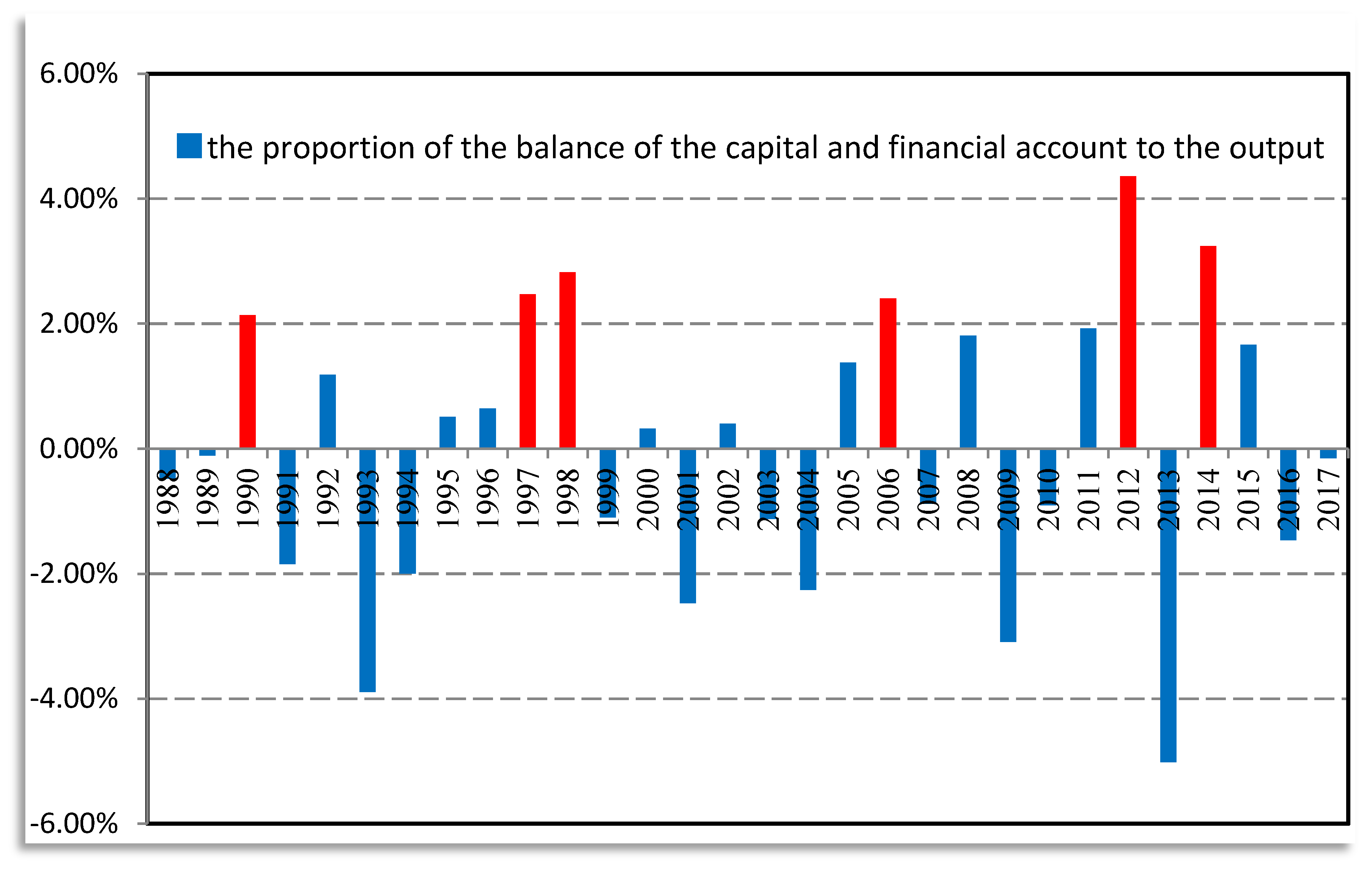
The JR model(the model of Jeanne and Rancière (2011))defines the sudden arrest of the capital inflow as the ratio of the capital and balance of the financial account ‘t’ of a country to the current output GDP of the country being more than 5% lower than t − 1. That is to say, if and , it will be considered that there is a sudden arrest of capital inflow in the t period of the country. To measure this probability, Jeanne and Rancière calculated the average probability of the occurrence of capital arrest in 34 middle-income countries in 1975–2003, and the result was 10%. In view of the situation of the capital arrest in China, this paper first calculates the number of the occurrence of capital arrest since the development of open economy in China. Since the relative value of π in the target period, 20 years, is slightly shorter in the calculation of this parameter, we choose the change trend of the proportion of the difference of Chinese capital and the financial account to the output in the 30 years between 1988 and 2017.
From Figure 1, we can see that in the 30-year period between 1988 and 2017, there is not a single year in which the proportion of the balance of capital and financial account to the output is consistent with the condition of the sudden arrest of capital inflow over the critical value of 5% under the JR model. This does not mean that the condition is unreasonable, but the situation in China is very special, and does not conform to the capital and financial account not being fully open. In fact, when Jeanne and Rancière (2011) defined the condition for the sudden arrest of the capital inflow, they directly referred to the related research (Guidotti et al., 2004) [29] of the existing scholars on the impact of capital arrest. According to Guidotti’s definition of “sudden arrest”, the decline in the balance of the capital and the financial account is measured by taking the next standard deviation relative to the mean value as the critical value; then, the critical value of 5% can be understood as the mean value of the threshold value of the sudden arrest of the capital inflow in global countries.
However, because the situation is different in different countries, it is difficult to accurately measure the situation of a single country with the same threshold value. So, we need to recalculate the threshold value with the same method especially for China. According to the sample of the 30 years between 1988 and 2017, the mean value of reducing the degree of, , the capital inflow ratio, k, is about 0.14%, and the standard deviation is about 2.24%. In combination with the reality of China, after fully considering that Chinese capital account are not fully open, there is still more strict control, the number of international capital imports and exports to China has been continuously increasing in recent years, and the impact on the economy and finance has become stronger and stronger, we set the critical value to 2%.
According to the critical value of 2%, in the 30 years between 1988 and 2017, the critical value of five years has exceeded 2%, and includes 1990, 1997, 1998, 2006, 2012 and 2015 (see the red part of the Figure 1). They all conform to the condition of the sudden arrest of Chinese capital inflow. Among them, the sudden arrest of the capital inflow in 1997 and 1998 was mainly caused by the Asian financial crisis, while the deficit in capital and financial accounts in 2006 was the result of the relaxation of the domestic capital outflows of countries. Of course, it also includes the reasons in the policy level of encouraging domestic enterprises to invest in foreign countries, increasing QDII (Qualified Domestic Institutional Investor), and so on. It is worth noticing that 2012 was the first year with the deficit in the annual capital and financial account since the 1998 crisis in China. Then, because of the capital flight caused by the United States (US) increasing the interest rate, the devaluation of the Chinese exchange rate, and other factors, there is the deficit again in 2015. However, no matter in which case, it will affect the consumption of the foreign exchange reserves of the government to offset the decline of net capital inflows. Therefore, considering the increasing frequency of the financial crisis in recent years, the increasing intensity of the contagion, the increasing uncertainty, the increasing possibility of large capital outflows, the further deepening of Chinese financial opening, and the increasing probability of the sudden arrest of capital inflows, the probability of the sudden arrest of capital inflows in the JR model is relatively conservative, and the probability of the sudden arrest of capital inflows in China is identified as π = 0.15 in this paper.
4.1.2. The Calculation of the Economic Growth Rate, g, and the Risk Aversion Coefficient, σ
This paper selects the mean of the annual rate of growth of GDP from 1994 to 2017 and gets the economic growth rate, g = 9.39% (National Bureau of Statistics http://www.stats.gov.cn/tjsj/).
The risk aversion coefficient, σ, is the only parameter that cannot be directly measured in the seven parameters. However, we can make reference to the existing research and international experience to measure it. Previous studies have shown that the risk aversion coefficient of representative consumers is valued between two and six (Yang Yi, Tao Yongcheng, 2011), and the greater the value, the higher the degree of risk aversion. The risk aversion coefficient in the JR model is calculated with the data of the emerging Asian market and set to two. Studies also show that the risk aversion coefficient of developing countries is generally higher than that of developed countries (Donadelli, Prosperi, 2012). Since Chinese investors are relatively conservative and the degree of risk aversion is higher, this paper takes as the risk aversion coefficient to calculate.
4.1.3. The Calculation of Short-Term Risk-Free Interest Rate, r, and Time Premium,
About 80% of Chinese external debt balance comes from international commercial loans, while the bonds of the foreign government account for a small proportion. In terms of currency composition, the ratio of US dollar debt is about 70%, which means that in the demand of the foreign exchange, the US dollar is still a relatively general and stable currency. In existing studies, the risk-free interest rate of short-term foreign debt is usually replaced by the interest rate of short-term US Treasury bonds. However, as the current short-term foreign debt is mainly composed of international trade credit financing and interbank credit, compared with the interest rate of US Treasury bonds, the LIBOR (London Inter-Bank Offer Rate) is more reasonable for calculating the lowest cost of the foreign debt that is in China’s possession. Here, this paper uses the weighted average r = 0.03 (StockQ database http://www.stockq.org/economy/libor.php) of the three-month LIBOR, and interest rates on three-month US Treasury bills within the last 20 years to calculate the interest rate level of holding short-term foreign debt.
The time premium, , represents the interest rate difference between long-term foreign debt and short-term foreign debt. The holding costs of Chinese long-term foreign debt are consistent with the US long-term treasury bonds. When the value of π is 0.1, it can be calculated that the average interest rate on 10-year US Treasury notes for nearly 20 years is 5% (US Treasury http://www.treasury.gov/resource-center/), so the time premium .
4.1.4. The Calculation of the Ratio of Short-Term Foreign Debt, λ, and the Rate of Output Loss, γ
According to the definition of the ratio of short-term foreign debt based on the GR model, we can calculate the ratio of short-term foreign debt to GDP for the 20 years between 1998 and 2017, and its average value λ = 6.24% (State Administration of Foreign Exchange http://www.safe.gov.cnzmodel_sarezindex.html). However, this only takes into account the demand of short-term foreign debts for foreign exchange reserves. In fact, China has medium and long-term foreign debts. It also has two ways of repayment. One is a one-time repayment at maturity. In this way, we should consider the maturity of the term within one year as a short-term bill. Another way is the annual amortization of medium and long-term foreign debts, and the part that is paid annually should also be regarded as a short-term bill. The two ways of repayment will make a large portion of the long-term foreign debts short-term, which will form short-term demand for foreign exchange reserves, while the GR model only considers the ratio of short-term foreign debts and estimates λ = 6.24%, significantly underestimating the effect of short-term foreign debts on foreign exchange reserves. Here, according to the condition of the medium and long-term external debt in China over the years, we assume that the average year is 10 years, allocate the total amount to the first year, consider the part whose time limit of the one-time repayment in the long-term foreign debt is within one year, and estimate the ratio of annual balance to GDP as about 3.5%. Therefore, combining short-term foreign debt and the short term of the medium and long-term debt, we determine the ratio of short-term foreign debt to be 8%.
The output loss rate, γ, is the loss when the sudden arrest of capital inflow occurs, and the output deviates from the original growth trajectory. When estimating the output loss rate in this paper, we will give full consideration to the impact of the sudden arrest of capital inflows and large amount of international capital outflows on China. On the one hand, from Figure 1, it can be seen that the sudden arrest of capital inflows in China in the last 30 years has occurred five times. Although the number is relatively low, in the context of the frequent international financial crisis of recent years, the probability of the sudden arrest of capital inflow will increase, and it will also accompany a large amount of international capital outflows at the same time. On the other hand, Chinese exports will be affected during the international financial crisis. For China, which has long pursued an export-oriented economic growth model, the financial crisis will inevitably affect the output. Based on these two considerations, we calculate the average γ of the decreasing amount of the output growth rate of 34 developing countries after the capital crisis calculated by the JR model as 6.5%, which is lower than the Chinese reality. Therefore, the output loss rate is set to 8.5% in this paper.
Based on the above analysis, the calculation results of each parameter can be summarized as follows (Table 1).
From Table 1, we can see that in combination with the reality of China, this paper calculates the original value of the JR model accordingly, which makes the model more convincing.
4.2. Solution of the Optimal Scale
Through the estimation of seven parameters, this paper will conduct the numerical simulation of the scale of Chinese optimal foreign exchange reserves under the framework of utility maximization, calculate the optimal scale of foreign exchange reserves, and compare it with the actual foreign exchange reserves.
First, we calculate the representative consumers’ consumption level in the period that the capital normally flows and compare it to the consumption marginal substitution rate P in the period of capital arrest:
Then, using Equation (20), .
It can be calculated .
Finally, take the ratio of ρ as the ratio of the scale of the optimal foreign exchange reserves and the output, and calculate the optimal scale of the foreign exchange reserves. The results are as follows.
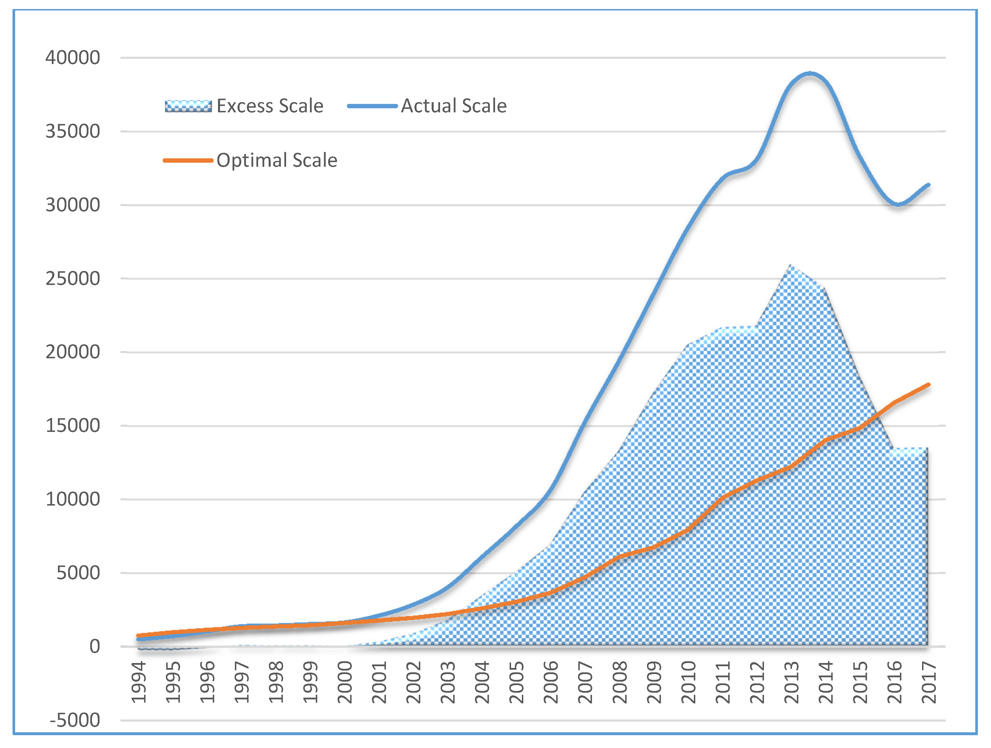
In order to be more intuitive, it can also be illustrated as shown in Figure 2.
It can be seen from Table 2 and Figure 2, that first of all, from the perspective of the scale of foreign exchange reserves, due to China’s reform of the foreign exchange system in 2005, and loosening the restrictions on capital flows, the scale of China’s foreign exchange reserves has also become the world’s largest foreign exchange reserves after breaking through the $1 trillion mark in 2006 and surpassing Japan, after which China has entered into a fast rising channel and reached a maximum value of $3 trillion and 840 billion in 2014, adding that the RMB(Renminbi) exchange rate continued to appreciate after 2005, forming a “double surplus” pattern under current account, capitaland financial account. Although it declined in 2015 and 2016, it rose again in 2017. At present, the scale of foreign exchange reserves has remained at around $3 trillion, but it is still operating at a high level.
Secondly, from the perspective of the optimal scale of the foreign exchange reserves, the optimal scale of China’s foreign exchange reserves has increased synchronously with the actual scale of foreign exchange reserves. However, its rise is relatively slow, and has does not changed significantly with the short-term changes in the actual scale of foreign exchange reserves. The optimal scale of foreign exchange reserves based on financial security has been greatly affected by external shocks; especially since the US financial crisis in 2008, the growth rate of the optimal scale of China’s foreign exchange reserves has been accelerating. However, the optimal scale of China’s foreign exchange reserves has not been reduced because of the decline in the scale of China’s actual foreign exchange reserves in 2015 and 2016. The major developed countries in the West entered the interest rate cycle in 2015; As a result, the fluctuations in the RMB exchange rate intensified and the signs of RMB depreciation emerged, leading to a massive outflow of the international capital from China and increasing financial risks. Therefore, from the perspective of the functional evolution of the foreign exchange reserves, the scale of foreign exchange reserves based on financial security will increase as the financial risks increase. The role of the foreign exchange reserves will become more and more obvious in maintaining the financial security of a country, which is consistent with the theoretical analysis of the previous article.
Finally, from the scale of excess foreign exchange reserves, before 1996, the actual scale of China’s foreign exchange reserves was absent. After 1996, with the rapid rise in the scale of China’s foreign exchange reserves, a large amount of excess foreign exchange reserves had been formed and fluctuated synchronously with the actual scale of foreign exchange reserves. At present, China’s foreign exchange reserves had obviously surpassed the most optimum output ratio, and thus, it fails to achieve the maximization of the social welfare utility. In other words, on the premise of the goal of financial stability and the maximization of the social welfare of the government, China’s actual foreign exchange reserves have gone beyond the optimal reserve scale since 2001. In 2017, the actual foreign exchange reserve of China was $3139.9 billion dollars. According to the calculation of this paper, the optimal foreign exchange reserve is $1782.4 billion dollars, while the excess foreign exchange reserve scale is $1357.6 billion dollars. Although the scale of Chinese foreign exchange reserves has fallen sharply since 2014, it still exceeded Chinese demand for foreign exchange reserves.
5. Conclusions and Enlightenment
To sum up, we can draw the following basic conclusions and enlightenment.
(1) With the rapid growth and the gathering of foreign exchange reserves in emerging markets, especially East Asian countries including China, the distribution of foreign exchange reserves has become increasingly uneven around the world. At the same time, with the increasing frequency of financial crises in recent years and more and more strong contagions, the special role of foreign exchange reserves in preventing financial risks and safeguarding national financial security has been fully recognized by most countries. The function of foreign exchange reserves has also shifted from simply meeting the needs of daily transactions to mainly meeting financial security demand. In China, the risks of foreign exchange reserves mainly lie in two aspects. On the one hand, the vast majority of China’s foreign exchange reserves are held in the form of foreign government bonds. Such bonds are relatively low in yields, and will lead to a depreciation of China’s foreign exchange reserve assets due to the devaluation of the currency of the issuer. This makes China’s foreign exchange reserves face higher risk and opportunity cost, thus making it trapped in the “double shrinkage” situation. On the other hand, a large number of foreign exchange reserves have forced the central bank to passively increase their supply of money, thus increasing the pressure of inflation and making it difficult for the central bank to implement monetary policy. Therefore, in this special historical period in which China holds huge foreign exchange reserves, we should give full play to the role of foreign exchange reserves in maintaining financial safety.
(2) This paper tries introducing the JR model. From the perspective of financial security, a theoretical analysis framework based on the maximization of utility is constructed on the basis of its correction. The framework takes the three-phase model of the external capital impact into the measurement process of the optimal scale of foreign exchange reserves, and introduces the social welfare function. Under the limit of the maximum of social welfare, we took a closed solution of the ratio of the optimal scale of foreign exchange reserves to output. This model is in line with the actual situation in which China is an open economy and an emerging market. It can integrate the risk factors of China’s financial instability into the estimation of the opportunity cost and welfare benefits of holding foreign exchange reserves, and the seven related important parameters can be depicted with the operation index of the Chinese open economy. Finally, it can also calculate the optimal ratio of Chinese foreign exchange reserves to GDP.
(3) This paper takes the change trend of the scale of Chinese foreign exchange reserves from 1994 to 2017 as the research object. The stages of the scale changes of Chinese foreign exchange reserve are divided. The direct reason for the rapid growth of the scale of Chinese foreign exchange reserves is mainly the inflow of interregional capital, which was caused by the structural plight of the double surplus of international balance of payments and the long-term appreciation expectation of the exchange rate. The deeper reason is that under the economic growth mode driven by Chinese exports, the excess foreign exchange cannot enter a mechanism of real economic growth. Since 2014, the reduction of foreign exchange reserves is mainly due to the economic recovery of the main developed countries in the West, especially in relation to the US entering the cycle of increasing the interest rate. In addition, the devaluation of Chinese RMB leads the international capital flow out from China and the exchange rate fluctuation aggravates, which threatens the financial security of China. Therefore, under the circumstance of the abnormal flow of international capital, we should give full play to the role of foreign exchange reserves in maintaining financial safety and preventing financial risks.
(4) The impact of the sudden arrest of capital inflows on the finance of a country has aroused wide attention from countries all over the world. Questions regarding how to deal with the impact of the sudden arrest of capital inflows and how much foreign exchange reserves needed are appropriate. The study of this paper gives a preliminary answer. Through parameter estimation and numerical simulation, the average optimal foreign exchange reserves scale of China between 1994 and 2017 was 13.53% of GDP. With this ratio as the standard, the Chinese foreign exchange reserve has shown a significant surplus since 2001. On the one hand, the holding of excess foreign exchange reserves and the rapid growth will inevitably cause the rising holding cost of China’s foreign exchange reserves, thus triggering the waste of resources and idle funds. On the other hand, the rapid growth of foreign exchange reserves aggravates the pressure of the appreciation of the RMB, which inevitably affects the international competitiveness of China’s export commodities. This shows that there are excess foreign exchange reserves in China, but foreign exchange reserves are not a case of the more, the better. Too much foreign exchange reserves will not only bring risks to China, they will also increase the holding cost. Therefore, how to manage foreign exchange reserves scientifically is still a difficult problem to be solved at present.
Author Contributions
G.Z. performed the theory analysis and contributed to drafting this manuscript. S.L. conceived and empirical analysis. X.Y. analyzed the data.
Acknowledgments
The research for this paper was supported by the National Natural Science Foundation of China (No. 71573050; No. 71573170) and the Shanghai Social Science Fund (No. 2015BJB003).
Conflicts of Interest
The authors declare no conflict of interest.
References
- Triffin, R. Gold and the Dollar Crisis: The Future of Convertibility; Yale University Press: New Haven, CT, USA, 1960. [Google Scholar]
- Jeanne, O.; Rancière, R. The Optimal Level of International Reserves for Emerging Market Countries: Formulas and Applications. IMF Working Paper, No. 6. 2006. Available online: https://www.google.com/url?sa=t&rct=j&q=&esrc=s&source=web&cd=1&ved=0ahUKEwiQ-fz77JXbAhVLerwKHYCSB8gQFggnMAA&url=https%3A%2F%2Fwww.imf.org%2Fexternal%2Fpubs%2Fft%2Fwp%2F2006%2Fwp06229.pdf&usg=AOvVaw3v7PcYfo6XVXeWSngL3a_d (accessed on 18 April 2018).
- Heller, H.R. Optimal international reserves. Econ. J. 1966, 302, 296–311. [Google Scholar] [CrossRef]
- Agarwal, J.P. Optimal monetary reserves for developing countries. Weltwirtschaftliches Arch. 1971, 107, 76–91. [Google Scholar] [CrossRef]
- Flanders, M.J. The Demand for International Reserves; Princeton University: Princeton, NJ, USA, 1971. [Google Scholar]
- Frenkel, J.A. The demand for international reserves by developed and less-developed countries. Economica 1974, 161, 14–24. [Google Scholar] [CrossRef]
- Iyoha, M.A. Demand for international reserves in less developed countries: A distributed lag specification. Rev. Econ. Stat. 1976, 3, 351–355. [Google Scholar] [CrossRef]
- Carbaugh, R.J.; Fan, L.S. The International Monetary System: History, Institutions, and Analyses; University Press of Kansas: Lawrence, KS, USA, 1976. [Google Scholar]
- Mendoza, R.U. International reserve-holding in the developing world: Self-insurance in a crisis-prone era? Emerg. Mark. Rev. 2004, 5, 61–82. [Google Scholar] [CrossRef]
- Aizenman, J.; Lee, J. International reserves: Precautionary versus mercantilist views, theory and evidence. Open Econ. Rev. 2007, 2, 191–214. [Google Scholar] [CrossRef]
- Jeanne, O.; Rancière, R. The Optimal Level of International Reserves for Emerging Market Countries: A New Formula and Some Applications. Econ. J. 2011, 555, 905–930. [Google Scholar] [CrossRef]
- Aizenman, J.; Edwards, S.; Riera-Crichton, D. Adjustment patterns to commodity terms of trade shocks: The role of exchange rate and international reserves policies. J. Int. Money Financ. 2012, 8, 1990–2016. [Google Scholar] [CrossRef]
- Aizenman, J.; Hutchison, M.M. Exchange market pressure and absorption by international reserves: Emerging markets and fear of reserve loss during the 2008–2009 crisis. J. Int. Money Financ. 2012, 31, 1076–1091. [Google Scholar] [CrossRef]
- Pina, G. The recent growth of international reserves in developing economies: A monetary perspective. J. Int. Money Financ. 2015, 58, 172–190. [Google Scholar] [CrossRef]
- Cova, P.; Pagano, P.; Pisani, M. Foreign exchange reserve diversification and the exorbitant privilege: Global macroeconomic effects. J. Int. Money Financ. 2016, 67, 82–101. [Google Scholar] [CrossRef]
- Pina, G. International reserves and global interest rates. J. Int. Money Financ. 2017, 74, 371–385. [Google Scholar] [CrossRef]
- Liu, B. Empirical Analysis of the Change of Foreign Exchange Reserves. Econ. Rev. 2003, 2, 114–117. [Google Scholar]
- Li, S. Measurement and Analysis of the Relative Scale of Chinese Foreign Trade Surplus: 1994–2004. Financ. Trade Econ. 2006, 1, 70–75. [Google Scholar]
- Wang, Q. Empirical Analysis of Moderate Scale of Chinese Foreign Exchange Reserves. Int. Financ. Res. 2008, 9, 73–79. [Google Scholar]
- Li, W.; Zhang, Z. A Framework for the analysis of foreign exchange reserves based on financial stability—On the moderate scale of chinese foreign exchange reserves. Econ. Res. 2009, 8, 27–36. [Google Scholar]
- Deng, C. Analysis of effective management of Chinese foreign exchange reserves. Manag. World 2016, 5, 170–171. [Google Scholar]
- Zhou, G.; Luo, S. Dynamic decision on the optimal scale of foreign exchange reserves—Analysis framework based on multilevel substitution effect. Financ. Res. 2011, 5, 29–41. [Google Scholar]
- Yang, Y.; Tao, Y. Measurement of appropriate scale of Chinese international reserves: 1994–2009. Int. Financ. Res. 2011, 6, 4–13. [Google Scholar]
- Wang, W.; Yang, J.; Wang, X.; Zhu, L. Development stage, exchange arrangement and the scale of Chinese high foreign exchange reserve. World Econ. 2016, 2, 23–47. [Google Scholar]
- Xiao, W.; Liu, L.; Liu, Y. Study on the moderate scale and the demand structure of Chinese foreign exchange reserves—Based on the revised Agarwal model. Financ. Trade Econ. 2012, 3, 46–52. [Google Scholar]
- Jiang, B.; Ren, F. A new exploration of the theory of the optimal foreign exchange reserve scale. Fudan J. (Soc. Sci. Ed.) 2013, 4, 10–16. [Google Scholar]
- Gong, J.; Gao, T.; Zhang, Z. The Asymmetric transfer effect of exchange rate fluctuations on chinese foreign exchange reserves—Based on the nonlinear LSTARX-GARCH model. Financ. Res. 2017, 2, 84–100. [Google Scholar]
- Lu, L.; Li, H.; Su, N. The optimal foreign exchange reserves and finance Open. Ref. Financ. Trade Econ. 2017, 12, 19–34. [Google Scholar]
- Guidotti, P.E. On the consequences of sudden stops. Economia 2004, 2, 171–214. [Google Scholar] [CrossRef]
Figure 1.
The proportion of the balance of the capital and financial account to the output. Data sources: China State Administration of Foreign Exchange and China National Bureau of Statistics.
Figure 1.
The proportion of the balance of the capital and financial account to the output. Data sources: China State Administration of Foreign Exchange and China National Bureau of Statistics.

Figure 2.
The Actual Scale and Optimal Scale of Chinese Foreign Exchange Reserves between 1994 and 2017. Data source: China National Administration of Foreign Exchange.
Figure 2.
The Actual Scale and Optimal Scale of Chinese Foreign Exchange Reserves between 1994 and 2017. Data source: China National Administration of Foreign Exchange.


Table 1.
Original Values and Calculated Values of Related Parameters.
| Related Parameters | Original Values of JR Model | Calculated Values of This Paper |
|---|---|---|
| Probability of Capital Sudden Arrest π | 0.1 | 0.15 |
| Economic Growth Rate g | 0.066 | 0.94 |
| Consumer Risk Aversion Coefficient σ | 2 | 5 |
| Short-term Risk-free Interest Rate r | 0.05 | 0.03 |
| Time Premium δ | 0.015 | 0.02 |
| Ratio of Short-term Foreign Debt λ | 0.107 | 0.08 |
| Output Loss Rate γ | 0.065 | 0.085 |
Table 2.
Comparison of Actual Scale of Foreign Exchange Reserves and Optimal Scale (Unit: 100 million dollars).
Table 2.
Comparison of Actual Scale of Foreign Exchange Reserves and Optimal Scale (Unit: 100 million dollars).
| Year | Actual Scale | Optimal Scale | Excess Scale |
|---|---|---|---|
| 1994 | 516.2 | 756.63 | −240.43 |
| 1995 | 735.97 | 984.96 | −248.99 |
| 1996 | 1050.29 | 1158.28 | −107.99 |
| 1997 | 1398.90 | 1288.94 | 109.96 |
| 1998 | 1449.59 | 1379.33 | 70.26 |
| 1999 | 1546.75 | 1465.68 | 81.07 |
| 2000 | 1655.74 | 1621.54 | 34.20 |
| 2001 | 2121.65 | 1792.48 | 329.17 |
| 2002 | 2864.07 | 1967.02 | 897.05 |
| 2003 | 4032.51 | 2220.23 | 1812.28 |
| 2004 | 6099.32 | 2613.51 | 3485.81 |
| 2005 | 8188.72 | 3054.56 | 5134.16 |
| 2006 | 10,663.44 | 3671.36 | 6992.08 |
| 2007 | 15,282.49 | 4729.63 | 10,552.86 |
| 2008 | 19,460.30 | 6118.03 | 13,342.27 |
| 2009 | 23,991.52 | 6752.18 | 17,239.34 |
| 2010 | 28,473.38 | 7954.37 | 20,519.01 |
| 2011 | 31,811.48 | 10,111.34 | 21,700.14 |
| 2012 | 33,115.89 | 11,305.52 | 21,810.37 |
| 2013 | 38,213.15 | 12,229.31 | 25,983.84 |
| 2014 | 38,430.18 | 14,044.65 | 24,385.53 |
| 2015 | 33,303.62 | 14,859.77 | 18,443.85 |
| 2016 | 30,105.17 | 16,579.63 | 13,525.54 |
| 2017 | 31,399.49 | 17,823.86 | 13,575.63 |
© 2018 by the authors. Licensee MDPI, Basel, Switzerland. This article is an open access article distributed under the terms and conditions of the Creative Commons Attribution (CC BY) license (http://creativecommons.org/licenses/by/4.0/).
Share and Cite
MDPI and ACS Style
Zhou, G.; Yan, X.; Luo, S. Financial Security and Optimal Scale of Foreign Exchange Reserve in China. Sustainability 2018, 10, 1724. https://doi.org/10.3390/su10061724
AMA Style
Zhou G, Yan X, Luo S. Financial Security and Optimal Scale of Foreign Exchange Reserve in China. Sustainability. 2018; 10(6):1724. https://doi.org/10.3390/su10061724
Chicago/Turabian StyleZhou, Guangyou, Xiaoxuan Yan, and Sumei Luo. 2018. "Financial Security and Optimal Scale of Foreign Exchange Reserve in China" Sustainability 10, no. 6: 1724. https://doi.org/10.3390/su10061724
Note that from the first issue of 2016, this journal uses article numbers instead of page numbers. See further details here.