Financial Hazard Map: Financial Vulnerability Predicted by a Random Forests Classification Model


Graduate School of Economics, Kobe University, 2-1, Rokkodai, Nada-Ku, Kobe 657-8501, Japan
*
Author to whom correspondence should be addressed.
Sustainability 2018, 10(5), 1530; https://doi.org/10.3390/su10051530
Submission received: 9 April 2018
/
Revised: 8 May 2018
/
Accepted: 8 May 2018
/
Published: 11 May 2018
(This article belongs to the Special Issue Risk Measures with Applications in Finance and Economics)
Abstract
:This study develops a systematic framework for assessing a country’s financial vulnerability using a predictive classification model of random forests. We introduce a new indicator that quantifies the potential loss in bank assets and measures a country’s overall vulnerability by aggregating these indicators across the banking sector. We also visualize the degree of vulnerability by creating a Financial Hazard Map that highlights countries and regions with underlying risks in their banking sectors.
1. Introduction
The severe economic consequences of the global financial crisis of 2008–2009 highlighted the importance of crisis prevention and sparked a renewed interest in early warning systems (EWSs). An EWS aims to detect potential vulnerabilities in a financial system that could trigger a system-wide crisis. A reliable EWS provides useful guidance for policy-makers to activate macro-prudential policy in an effective and timely manner. The International Monetary Fund (IMF) [1] and the Committee on the Global Financial System [2] provide a comprehensive discussion of the operational aspects of the macro-prudential policy. After Frankel and Rose [3] and Kaminsky et al.’s [4] early contributions, researchers have made considerable efforts to develop a consistently useful EWS for various types of crises.
Kaminsky et al. [4] proposed the popular signaling approach, which Alessi and Detken [5] recently used. This approach seeks to identify the threshold values for individual indicators that signal crises, and thus trigger an early warning when the pre-defined threshold for the pre-selected indicator is breached. A popular indicator common in these studies is the credit-to-GDP (Gross Domestic Product) ratio, which is a key indicator signaling credit booms. However, this signaling approach has a shortcoming given that, as a univariate approach, the decision would rely on only a single factor, which can send a misleading signal.
Another conventional approach from the EWS literature is estimating the multivariate probit and logistic regressions, which relate the probability of a crisis to a set of explanatory variables, such as current account balance, real exchange rates, credit growth, and fiscal balance [6,7,8,9,10]. Despite its popularity, the conventional approach has certain limitations. For one, researchers must pre-select explanatory variables from a wide range of economic indicators based on some prior information. For another, the logistic regression does not readily allow for non-linear or threshold effects of explanatory variables. More generally, linear regressions often perform poorly in terms of prediction performance relative to newer machine learning models [11]. Linear regressions may work well for small datasets but they are not readily scalable to larger datasets.
Ghosh and Ghosh [12] and Frankel and Wei [13] employed a decision tree method that uses a sequence of splitting rules to segment the space of explanatory variables. Hastie et al. [11] and James et al. [14] provide details of tree methods, including decision trees and random forests. At each node of a tree, the sample is split into two sub-branches according to the threshold value of an explanatory variable. For classification trees, either the Gini index or the cross entropy is used to evaluate the quality of a split. A smaller value of these indices indicates that the node is purer, and thus contains more observations from a single class. The process is repeated until a stopping criterion is reached, such as the minimum number of observations at each node. Each terminal node at the bottom of the tree provides a class prediction for a given observation. Whereas linear logistic regressions models require a handcrafted selection of explanatory variables to obtain reasonable early warning performance, the decision tree systematically learns important variables, performs better in early warning, and allows for non-linear effects. Although a decision tree is simple and provides explanatory and intuitive decision rules, it suffers from high variance (i.e., a small change in the data can cause a large change in the financial tree), so is likely to suffer over-fitting problems. This is largely owing to the fact that the values of the thresholds depend heavily on the values of the training observations.
With an increased opportunity to gain access to larger datasets, exploring the significant scope for economic modeling and analysis for a more flexible approach has become popular with data scientists [15,16]. In this study, we take advantage of the advancements in predictive modeling techniques of machine learning to build an EWS, and develop a systematic framework to assess and visualize a country’s financial vulnerability. The main contributions of our study are three-fold. First, our study differs from previous ones in that we used a novel machine-learning technique known as random forests to construct an EWS to predict bank failures (random forests EWS). Random forests are a variant of decision trees that significantly improve prediction accuracy by combining a large number of trees using random input selection [17]. Second, we introduce a new indicator that quantifies the expected potential loss in bank assets computed using the prediction of the random forests EWS. To assess a country’s overall financial vulnerability, we aggregate individual banks’ expected potential asset losses across the domestic banking sector. Finally, we visualize the degree of a country’s financial vulnerability by creating a Financial Hazard Map that highlights countries and regions with significant risks in their underlying banking sectors. Our work is similar to that of Tanaka et al. [18], but differs by a few points. Our paper provides a financial analysis of the finance sector, whereas the interest of Tanaka et al. focused on the industrial sector. Furthermore, we propose a novel indicator to assess the overall financial vulnerability of each country.
We chose random forests (RF) for three reasons. First, RF can significantly improve prediction accuracy by building a large number of decision trees on bootstrapped training samples—a technique known as ensemble learning. Random forests also circumvent the over-fitting problem by adding randomness to the tree building process, and thus reducing correlations among trees; hence, it performs well with out-of-sample data. Second, random forests can better handle a large dataset as multiple trees can be trained in parallel efficiently with a very simple hyper-parameter setting. The model can be built by merely setting the number of trees. Finally, RF provide the importance measurement, which can be used for certain levels of causality inference. Whereas various application areas use random forests, including computer vision and bioinformatics, its application to economics remains limited. Tanaka et al. [19] used random forests to predict bank failure in OECD member countries.
Another important feature of our study is the use of bank-level financial statements to predict bank failure using the random forests EWS built from a large dataset of more than 15,000 banks globally. As previous studies typically used macroeconomic indicators to predict currency and financial crises, the recent literature indicates that the state of bank financial statements can explain differences in performance across banks during financial crises [20,21]. Moreover, previous studies often defined a crisis as an event in which the values of preselected indicators exceed predetermined thresholds. Consequently, the prediction performance significantly depends on the choice of threshold. We define the event of a bank failure as the change in a bank’s status from active to inactive (i.e., bankrupt, in liquidation, or dissolved) based on the information provided by the Bureau Van Dijk Bankscope. By doing so, we wanted to minimize arbitrariness, and thus reduce the possible bias in prediction.
The remainder of the paper proceeds as follows. Section 2 describes the methodology and data of building the random forests EWS. Section 3 introduces a new indicator that quantifies the expected potential losses in bank assets. We present the assessment of a country’s financial vulnerability and visualize it by creating a Financial Hazard Map. Section 4 provides our conclusions.
2. Materials and Methods
In this study, we considered the task of building an EWS as a classification problem to identify a bank’s status (i.e., active or inactive) based on the underlying financial conditions. Drawing on insights from the extensive literature on corporate bankruptcy predictions, we used information about individual banks’ financial statements as predictors to build models. Altman [22] provides an early contribution to the literature. In contrast to existing studies that are more concerned with identifying the key predictors of bankruptcy, we prioritized improving the prediction accuracy. To this end, we used random forests that tend to perform better in terms of prediction accuracy than conventional methods, such as logistic regressions, which have been widely used in previous studies.
2.1. Major Features of Random Forests
Random forests are a variant of decision trees, which overcome the over-fitting problem by building multiple trees and combing the results of these trees [17], effectively forming forests. Each tree in a random forest is built using randomly selected data samples and/or randomly selected input variables from the original data to split each node. After generating a large number of trees, the model votes for the most popular class. A single-tree classifier tends to have only marginally better accuracy than a random choice of class. However, by combining a large number of trees using random input selection, random forests can produce a powerful model.
Breiman et al. [17] constructed such trees using the Gini index criterion, which measures the best split criterion based on the impurity of each node. The algorithm aims to select the optimal splitting variable and the corresponding threshold value by making each node as pure as possible. Suppose is the number of pieces of information reaching node n and is the number of data points belonging to class , the Gini index, , of node n is obtained using Equation (1):
A smaller Gini index value for node n represents greater purity, which implies that the node contains more observations from a single class. Hence, a decreasing Gini index is an important criterion when splitting a node.
In comparison to single-tree modeling, random forests have several desirable features [17,23]. First, random forests perform better in terms of classification accuracy by building a large number of trees instead of only a single tree. Each tree is built using randomly selected data samples and randomly selected input variables from the original data to split each node. After generating a large number of trees, they vote for the most popular class. A single-tree classifier tends to have only marginally better accuracy than a random choice of class. However, by combining a large number of trees using random input selection, random forests can improve accuracy. Second, random forests provide better generalization abilities and are robust to over-fitting. Hence, RF may have better out-of-sample accuracy when using a random selection of input variables to split each node and combining the results of multiple trees yields error rates that compare favorably to alternative methods and are more robust with respect to noise. Third, random forests can better handle large datasets as multiple trees can be efficiently trained in parallel. Finally, random forests provide a measure for the relative contribution of each variable to generate a prediction. These variable importance measures help identify the variables that are important for distinguishing between active and inactive banks, and thus for predicting bank failure.
2.2. Data
We sourced our data for bank financial statement indicators from Bankscope. The advantage of using this data source is that it provides a broad coverage of banks with standardized data formats across countries. We used 48 indicators derived from the Summary Analytics category classified into four groups: profitability ratio, capitalization, loan quality, and funding (Appendix B). Our sample included 23,455 commercial banks, saving banks, and cooperatives incorporated in 198 countries and regions. The training set included annual observations of the latest available financial statements for each bank up to 2014. We defined a bank failure event as the change in a bank’s status from active to inactive (i.e., bankrupt, in liquidation, or dissolved) as reported by Bankscope. We assumed that the latest available financial statements for active banks had sound financial status and inactive banks had unsound financial status. We then systematically identified patterns distinguishing the differences by random forests.
As there were fewer inactive banks (7294 banks), we selected the largest 7294 active banks in terms of total assets to match the number of inactive banks. We also selected the smallest 7294 active banks to build a more flexible model to prevent a bias toward larger banks. To avoid model bias created by an imbalanced training set, we evened out the sample sizes of active and inactive banks by doubling the sample size of inactive banks by duplicating each observation. In addition, we eliminated variables if more than 50% of its values were missing (7294 × 2 biggest and smallest active banks + 7294 inactive banks). Thus, we eliminated 6 variables and used 42 variables for experiments. We used the random forests and caret packages in the R software package to train and evaluate our models. Figure 1 illustrates the model building process for the random forests EWS. Appendix C reports the classification accuracy of the random forests EWS.
3. Results
3.1. Variable Importance Measures
A useful property of random forests is that it provides variable importance measures that help identify the most important variables for distinguishing between active and inactive banks. Hence, RF should provide some clues to the underlying causes of bank failures. For classification trees, we obtained the variable importance measures from each variable’s contribution to the reduction in the Gini index. The Gini index is a common measure of the degree of inequality in income distribution. The smaller the value of the index, the more equal the society.
In our random forests algorithm, the Gini index is the measure for the purity of each node. A smaller value of the Gini index represents a purer node, which implies that the node contains more observations from a single class. The goal of the algorithm was to make each node as pure as possible by selecting the optimal splitting variable and the corresponding threshold value. Therefore, we calculated variable importance by summing the total reduction in the Gini index by splits over a given variable, averaged over all bagged trees.
Figure 2 illustrates the variable importance measures as the mean decrease in the Gini index for each variable. Considering this model, we identified the following indicators as the top four predictors: interest expense/average interest-bearing liabilities, interest income on loan/average gross loans, interest expense on customer deposits/average customer deposits, and interest income/average earning assets. The importance measure for the first indicator was by far the largest. These top four indicators fall into the profitability ratio category. In contrast, the importance measures for the other categories of indicators, that is, capitalization, loan quality, and liquidity are much smaller. The results indicate that bank profitability has the most important impact on the probability of bank failure.
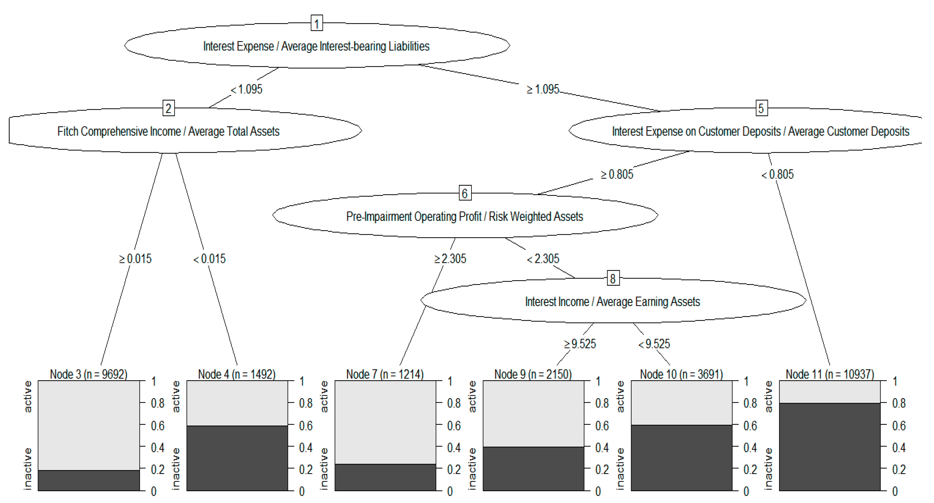
We show the experimental result of a single decision tree in Figure 3 for comparison. Though a single tree selects similar criteria to distinguish between active and inactive banks, it does not perform as well as random forests. This is due to the fact that the random forests model produces a more flexible model as it produces multiple trees to analyze different patterns in the data, whereas a single tree only produces one set of rules for a classification decision.
3.2. New Indicator for the Expected Potential Asset Loss
We introduce a new indicator to assess the degree of financial vulnerability using the prediction of the random forests EWS. We used the 2014 financial statement data to predict the probability of bank failure. We define the expected potential asset loss of a bank as follows:
where EPALi,j denotes the expected potential loss in bank i in country j, Pi,j denotes the probability of failure for bank i in country j given by the random forests EWS prediction, and Total Assetsi,j denotes the value of total assets of bank i in country j. To measure a country’s overall financial vulnerability, we aggregate the value of EPALi,j across the domestic banking sector. Given that we used consolidated financial statement data, all the expected potential loss of multinational banks was counted as losses in the country where the headquarters of these banks were located. We acknowledge that this is the limitation of our work and consider overcoming this limitation as our future task. Hence, the country-level expected potential loss in the domestic banking sector denoted by EPALj is given by:
EPALi,j = Pi,j × Total Assetsi,j,
EPALj = ∑i EPALi,j.
To gauge the impact of the expected potential asset loss on the domestic banking sector and economic activities, we calculated the share of EPALj in the total assets of the domestic banking sector and in nominal GDP. Table 1 summarizes the results.
The left column of the table ranks 50 countries in terms of their share in banking sector assets. The ranking indicates that Suriname, Grenada, Denmark, Gabo, and Guatemala are the five most vulnerable countries in the sense that the impact of the expected potential loss on the domestic banking sector can be relatively large. Thus, these countries have a relatively high risk of a system-wide banking crisis.
The right column of the table ranks countries in terms of the share in nominal GDP. The ranking indicates that the Palestinian Territories, Luxembourg, Cyprus, Denmark, and France are the five most vulnerable countries in the sense that the impact of the expected potential asset loss on domestic economic activities could be relatively large. This is particularly the case if the assets of banks with high probability of failure consist primarily of domestic loans and investments.
Interestingly, many Organisation for Economic Co-operation and Development (OECD) countries, including European countries, at the top of the list. This may indicate that these countries have not recovered fully from the major financial crises, notably, the global financial crisis of 2008–2009 and the European debt crisis of 2010–2013, or new financial risks may be looming. Given the relatively large size of their domestic banking sectors, these countries can be the epicenter of cross-border financial spillovers by withdrawing overseas loans and investments in the face of financial difficulties.
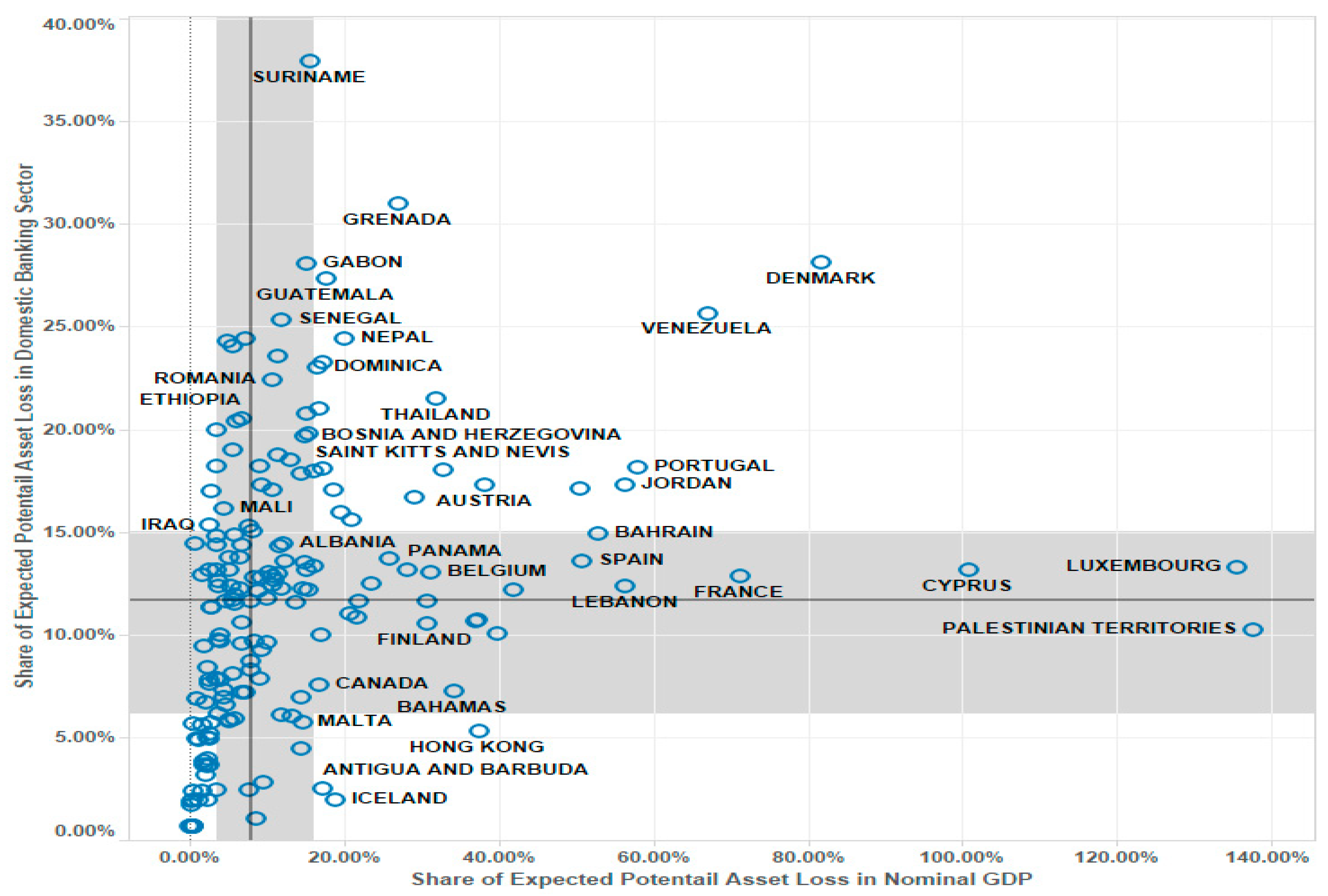
In Figure 4, we create a scatter plot of the vulnerability measures reported in Table 1. The combination of higher values of these measures in a particular country implies greater financial vulnerability. The figure clearly indicates that Denmark and Venezuela stand out in terms of both measures, signaling significant risks. The bold horizontal and vertical lines indicate the medians of these measures; the shadows indicate the first quartiles. The medians of the share of EPALj in the banking sector assets and nominal GDP are 11.60% and 7.85%, respectively. The level of these medians indicates the overall vulnerability of the global banking sector, with a significant increase in signaling financial risks. Notably, our vulnerability measure raises a red flag for potential trouble, but it does not identify the causes or the likely outcomes of the trouble. However, we believe that these measures are useful for spotting vulnerabilities, and thus encouraging regulators and investors to take preemptive actions.
In Appendix A, we summarize the predicted bank failures for each country for 2014. The table shows the number of banks and the sum of assets held by the banks for each category of predicted probability of failures with a 10-percentage-point interval.
3.3. Financial Hazard Map
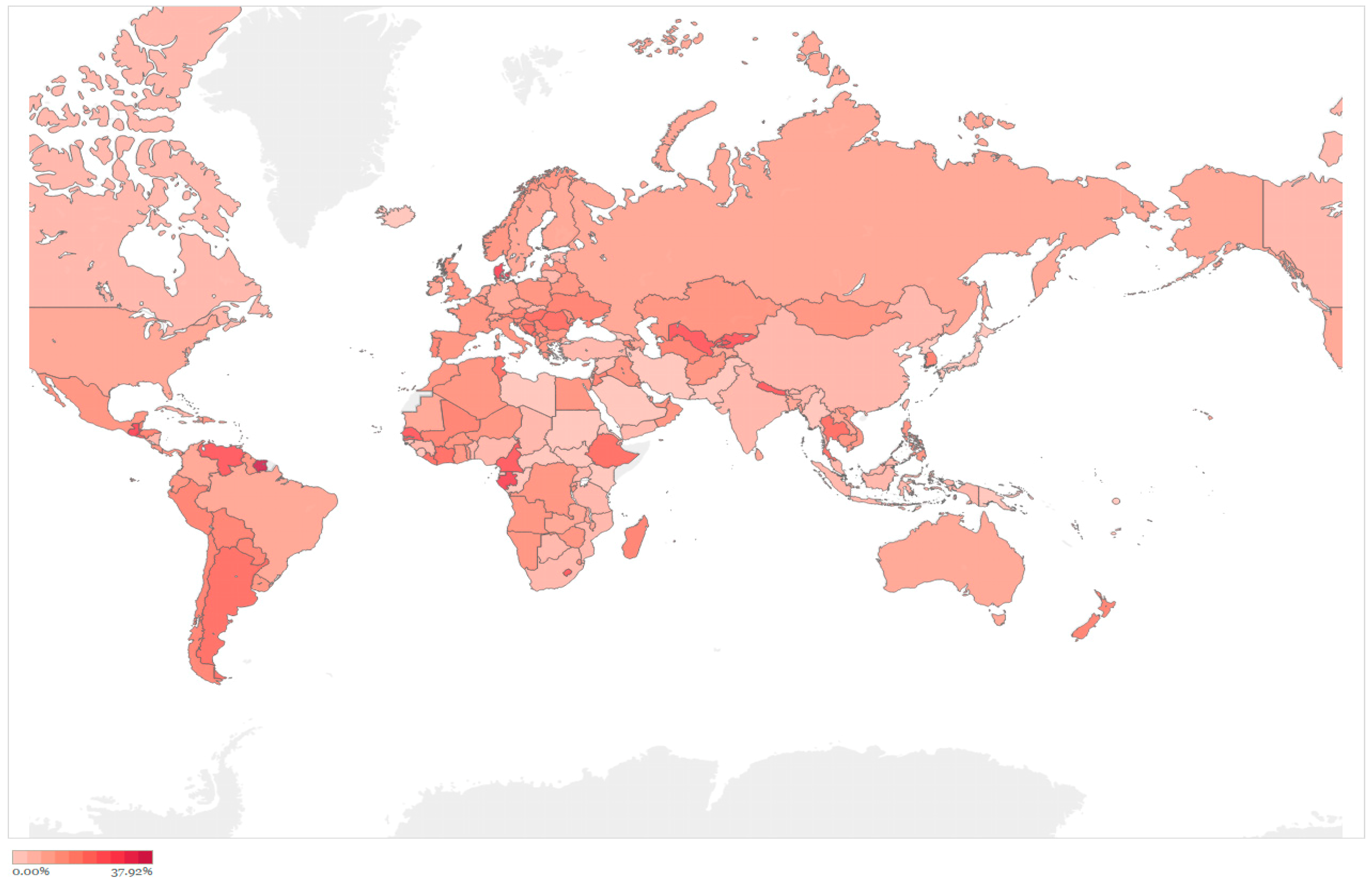
Finally, we visualized the degree of a country’s financial vulnerability by creating a Financial Hazard Map. Corresponding to each definition of vulnerability in Table 1, we present two types of maps. Figure 5 shows the share of EPALj in the assets of domestic banking sectors. The areas that are darker red indicate a higher degree of vulnerability in terms of the impact of the expected potential asset loss on the domestic banking sector. Figure 6 shows the share of EPALj in nominal GDP. Darker red areas indicate a higher degree of vulnerability in terms of the impact of the expected potential asset loss on domestic economic activities.
The Financial Hazard Map highlights countries and regions with significant vulnerability in their underlying banking sector. The darker red areas correspond to the top 50 countries listed in Table 1. The map provides a clear and understandable assessment of financial vulnerability in particular countries and regions. It also shows the geographical distribution of financial risk and the danger of potential contagion for neighbors of high vulnerability areas.
4. Conclusions
We developed a systematic framework for assessing and visualizing a country’s financial vulnerability. We employed a novel machine-learning approach known as random forests to construct an EWS to predict bank failures and introduced a new indicator that quantifies the expected potential loss in bank assets computed based on the random forests EWS prediction. We assessed the financial vulnerability of each country by aggregating individual banks’ indicators across the banking sector. To gauge the impact of expected potential asset loss, we calculated the shares in the banking sector assets and nominal GDP. We identified countries and regions with high vulnerability in terms of these shares. Furthermore, we visualized the degree of a country’s financial vulnerability by creating a Financial Hazard Map. We demonstrated the usefulness of the Financial Hazard Map in spotting vulnerable countries and regions and understanding the geographical distribution of risk.
We hope that the Financial Hazard Map will prove useful for both policy-makers and private investors in detecting potential risk, and thereby prompting precautionary actions. Our framework of assessing financial vulnerability is simple, and therefore readily applicable to other types of risk analysis. A future task may be to develop a dynamic framework that allows for an assessment of contagion risks between banks and countries potentially in trouble, taking account of country-specific macroeconomic and institutional factors.
Author Contributions
S.H. and T.K. conceived and designed the experiments; K.T. performed the experiments; S.H., T.K. and K.T. analyzed the data; K.T. contributed reagents/materials/analysis tools; K.T. wrote the paper.
Acknowledgments
We are grateful to four anonymous referees for their helpful comments and suggestions. This work is supported by JSPS KAKENHI Grant Number 17K18564 and 17H00983.
Conflicts of Interest
The authors declare no conflict of interest. The founding sponsors had no role in the design of the study; in the collection, analyses, or interpretation of data; in the writing of the manuscript, and in the decision to publish the results.
Appendix A
Numbers and assets of banks for each category of bank failure probabilities.


Appendix B
List of variables used to build the random forests EWS.
List of incorporated bank-level variables
- Interest Income on Loans/Average Gross Loans
- Interest Expense on Customer Deposits/Average Customer Deposits
- Interest Income/Average Earning Assets
- Interest Expense/Average Interest-bearing Liabilities
- Net Interest Income/Average Earning Assets
- Net Int. Increase Less Loan Impairment Charges/Average Earning Assets
- Net Interest Increase Less Preferred Stock Dividend/Average Earning Assets
- Non-Interest Income/Gross Revenues
- Non-Interest Expense/Gross Revenues
- Non-Interest Expense/Average Assets
- Pre-impairment Operating Profit/Average Equity
- Pre-impairment Operating Profit/Average Total Assets
- Loans and securities impairment charges/Pre-impairment Operating Profit
- Operating Profit/Average Equity
- Operating Profit/Average Total Assets
- Taxes/Pre-tax Profit
- Pre-Impairment Operating Profit/Risk Weighted Assets
- Operating Profit/Risk Weighted Assets
- Net Income/Average Total Equity
- Net Income/Average Total Assets
- Fitch Comprehensive Income/Average Total Equity
- Fitch Comprehensive Income/Average Total Assets
- Net Income/Risk Weighted Assets
- Fitch Comprehensive Income/Risk Weighted Assets
- Tangible Common Equity/Tangible Assets
- Tier 1 Regulatory Capital Ratio
- Total Regulatory Capital Ratio
- Equity/Total Assets
- Cash Dividends Paid and Declared/Net Income
- Cash Dividend Paid and Declared/Fitch Comprehensive Income
- Net Income–Cash Dividends/Total Equity
- Growth of Total Assets
- Growth of Gross Loans
- Impaired Loans (NPLs)/Gross Loans
- Reserves for Impaired Loans/Gross loans
- Reserves for Impaired Loans/Impaired Loans
- Impaired Loans less Reserves for Impaired Loans/Equity
- Loan Impairment Charges/Average Gross Loans
- Net Charge-offs/Average Gross Loans
- Impaired Loans + Foreclosed Assets/Gross Loans + Foreclosed Assets
- Loans/Customer Deposits
- Customer Deposits/Total Funding excluding Derivatives
List of eliminated bank-level variables (variables with missing values more than 50% of observations)
- Net Income/Average Total Assets + Average Managed Securitized Assets
- Fitch Core Capital/Weighted Risks
- Fitch Eligible Capital/Weighted Risks
- Core Tier 1 Regulatory Capital Ratio
- Cash Dividends and Share Repurchase/Net Income
- Interbank Assets/Interbank Liabilities
Appendix C
Evaluating classification accuracy
To evaluate the classification accuracy of the random forests EWS, we used K-fold cross-validation, which is a standard resampling technique used for estimating model performance. The basic idea involves using parts of the sample data to fit the model (training set) and the remaining part to estimate the prediction error of the model (validation set). First, we randomly split the observations into K folds of roughly equal size. Then, we treated one of the K folds as a validation set and fit the model on the remaining K–1 folds. We calculated the prediction error of the observations in the validation set. We repeated the process K times to obtain K different estimates of the prediction error. The K-fold cross-validation estimate of the prediction error is the average of these values. Since the typical choice of K is either 5 or 10, we used a 10-fold cross-validation. Using the same setup, we compared the performance of the random forests EWS with that of conventional EWSs based on a logistic regression and a decision tree. The random forests model produced an accuracy rate of 93.64%, whereas the logistic regression and decision tree produced accuracy rates of 65.73% and 73.75%, respectively. The result clearly indicates that random forests can build more reliable EWSs than conventional methods.
We also conducted a historical back test to evaluate the classification accuracy. More specifically, we predicted the bank status (active or inactive) in 2013 and 2014 based on banks’ financial statements in 2013, excluding those that became inactive before 2013. We evaluated performance in terms of accuracy by comparing the predicted bank status with the actual status in 2013 and 2014. The random forests model produced an accuracy rate of 85.27%, whereas the logistic regression and decision tree produce accuracy rates of 53.44% and 56.43%, respectively. Once again, the result clearly indicates that the random forest EWS outperforms the conventional EWSs.
References
- International Monetary Fund (IMF). Macroprudential Policy: An Organizing Framework; International Monetary Fund: Washington, DC, USA, March 2011. [Google Scholar]
- Committee on the Global Financial System. Operationalising the Selection and Application of Macroprudential Instruments; CGFS Paper No. 48; Bank for International Settlements: Basel, Switzerland, December 2012. [Google Scholar]
- Frankel, J.A.; Rose, A.K. Currency crashes in emerging markets: An empirical treatment. J. Int. Econ. 1996, 41, 351–366. [Google Scholar] [CrossRef]
- Kaminsky, G.L.; Lizondo, S.; Reinhart, C.M. The leading indicators of currency crises. IMF Staff Pap. 1998, 45, 1–48. [Google Scholar] [CrossRef] [Green Version]
- Alessi, L.; Detken, C. Identifying Excessive Credit Growth and Leverage; ECB Working Paper No. 1723; European Central Bank: Frankfurt, Germany, August 2014. [Google Scholar]
- Bussiere, M.; Fratzscher, M. Towards a new early warning system of financial crises. J. Int. Money Financ. 2006, 25, 953–973. [Google Scholar] [CrossRef]
- Rose, A.K.; Spiegel, M.M. Cross-country causes and consequences of the crisis: An update. Eur. Econ. Rev. 2011, 55, 309–324. [Google Scholar] [CrossRef]
- Frankel, J.; Saravelos, G. Can leading indicators assess country vulnerability? Evidence from the 2008–2009 global financial crisis. J. Int. Econ. 2012, 87, 216–231. [Google Scholar] [CrossRef]
- Duca, M.L.; Peltonen, T.A. Assessing systemic risks and predicting systemic events. J. Bank. Financ. 2013, 37, 2183–2195. [Google Scholar] [CrossRef]
- Mathias, D.; Mikael, J. Evaluating early warning indicators of banking crisis: Satisfying policy requirements. Int. J. Forecast. 2014, 30, 759–780. [Google Scholar]
- Hastie, T.; Tibshirani, R.; Friedman, J. The Elements of Statistical Learning; Springer: New York, NY, USA, 2008. [Google Scholar]
- Ghosh, S.R.; Ghosh, A.R. Structural vulnerabilities and currency crises. IMF Staff Pap. 2002, 50, 481–506. [Google Scholar] [CrossRef]
- Frankel, J.; Wei, S.-J. Managing macroeconomic crises: Policy lessons. In Managing Economic Volatility and Crises: A Practitioner’s Guide; Aizenman, J., Pinto, B., Eds.; Cambridge University Press: Cambridge, UK, 2005; pp. 315–405. [Google Scholar]
- James, G.; Witten, D.; Hastie, T.; Tibshirani, R. An Introduction to Statistical Learning; Springer: New York, NY, USA, 2013. [Google Scholar]
- Varian, H.R. Big data: New tricks for econometrics. J. Econ. Perspect. 2014, 28, 3–28. [Google Scholar] [CrossRef]
- Einav, L.; Levin, J. The data revolution and economic analysis. Innov. Policy Econ. 2014, 14, 1–24. [Google Scholar] [CrossRef]
- Breiman, L. Random forests. Mach. Learn. 2001, 45, 5–32. [Google Scholar] [CrossRef]
- Tanaka, K.; Higashide, T.; Kinkyo, T.; Hamori, S. Forecasting the Vulnerability of Industrial Economic Activities: Predicting the Bankruptcy of Companies. J. Manag. Inf. Decis. Sci. 2017, 20, 1–24. [Google Scholar]
- Tanaka, K.; Kinkyo, T.; Hamori, S. Random forests-based early warning system for bank failures. Econ. Lett. 2016, 148, 118–121. [Google Scholar] [CrossRef]
- Berger, A.N.; Bouwman, C.H.S. How does capital affect bank performance during financial crises? J. Financ. Econ. 2013, 109, 146–176. [Google Scholar] [CrossRef]
- Vazquez, F.; Federico, P. Bank funding structures and risk: Evidence from the global financial crisis. J. Bank. Financ. 2015, 61, 1–14. [Google Scholar] [CrossRef]
- Altman, E.I. Financial ratios, discriminant analysis and the prediction of corporate bankruptcy. J. Financ. 1968, 23, 189–209. [Google Scholar] [CrossRef]
- Kuhn, M.; Johnson, K. Applied Predictive Modeling; Springer: New York, NY, USA, 2013. [Google Scholar]
Figure 1.
Model building process of random forests early warning system (EWS).

Figure 2.
Variable importance measures of random forests.

Figure 3.
Plot of a tree model.

Figure 4.
Scatter plot of country vulnerabilities.

Figure 5.
Impact of expected potential asset loss on the banking sector.

Figure 6.
Impact of expected potential asset loss on economic activities.


Table 1.
Top 50 countries in terms of the shares of expected potential asset loss based on 2014 financial statements.
Table 1.
Top 50 countries in terms of the shares of expected potential asset loss based on 2014 financial statements.
| Share of Expected Potential Asset Loss in Domestic Banking Sector | Share of Expected Potential Asset Loss in Nominal GDP | ||
|---|---|---|---|
| SURINAME | 37.92% | PALESTINIAN TERRITORIES | 137.53% |
| GRENADA | 31.00% | LUXEMBOURG | 135.54% |
| DENMARK | 28.14% | CYPRUS | 100.92% |
| GABON | 28.06% | DENMARK | 81.80% |
| GUATEMALA | 27.33% | FRANCE | 71.26% |
| VENEZUELA | 25.65% | VENEZUELA | 67.12% |
| SENEGAL | 25.30% | PORTUGAL | 58.03% |
| NEPAL | 24.41% | LEBANON | 56.36% |
| UZBEKISTAN | 24.41% | JORDAN | 56.25% |
| KYRGYZSTAN | 24.31% | BAHRAIN | 52.90% |
| CAMEROON | 24.04% | SPAIN | 50.81% |
| LESOTHO | 23.54% | MAURITIUS | 50.56% |
| EL SALVADOR | 23.25% | UNITED KINGDOM | 41.92% |
| DOMINICA | 23.00% | SWITZERLAND | 39.83% |
| ROMANIA | 22.44% | AUSTRIA | 38.16% |
| THAILAND | 21.48% | HONG KONG | 37.43% |
| HUNGARY | 20.99% | GERMANY | 37.28% |
| MONTENEGRO | 20.74% | NETHERLANDS | 36.94% |
| ETHIOPIA | 20.51% | BAHAMAS | 34.16% |
| ARGENTINA | 20.38% | SAINT KITTS AND NEVIS | 32.75% |
| LIBERIA | 19.95% | THAILAND | 31.86% |
| TUNISIA | 19.81% | BELGIUM | 31.19% |
| LIECHTENSTEIN | 19.72% | FINLAND | 30.61% |
| BOSNIA AND HERZEGOVINA | 19.66% | SAN MARINO | 30.59% |
| COTE D'IVOIRE | 19.01% | NEW ZEALAND | 28.96% |
| PARAGUAY | 18.75% | PANAMA | 28.10% |
| SERBIA | 18.50% | GRENADA | 27.02% |
| MADAGASCAR | 18.22% | ITALY | 25.76% |
| BOLIVIA | 18.17% | GREECE | 23.50% |
| PORTUGAL | 18.17% | MOROCCO | 21.80% |
| REPUBLIC OF KOREA | 18.09% | AUSTRALIA | 21.56% |
| SAINT KITTS AND NEVIS | 17.99% | CHILE | 20.94% |
| HONDURAS | 17.96% | IRELAND | 20.55% |
| BELIZE | 17.81% | NEPAL | 19.99% |
| PERU | 17.30% | CROATIA | 19.43% |
| AUSTRIA | 17.30% | ICELAND | 18.82% |
| JORDAN | 17.27% | CAPE VERDE | 18.66% |
| MAURITIUS | 17.13% | GUATEMALA | 17.61% |
| UKRAINE | 17.05% | REPUBLIC OF KOREA | 17.19% |
| CAPE VERDE | 17.03% | EL SALVADOR | 17.05% |
| TURKMENISTAN | 16.96% | ANTIGUA AND BARBUDA | 17.03% |
| NEW ZEALAND | 16.70% | SWEDEN | 16.97% |
| MALI | 16.15% | CANADA | 16.74% |
| CROATIA | 15.97% | HUNGARY | 16.69% |
| CHILE | 15.60% | DOMINICA | 16.46% |
| BRUNEI DARUSSALAM | 15.33% | HONDURAS | 16.04% |
| ARMENIA | 15.30% | BARBADOS | 15.89% |
| DOMINICAN REPUBLIC | 15.04% | SURINAME | 15.52% |
| BAHRAIN | 14.89% | VIETNAM | 15.34% |
| ECUADOR | 14.84% | TUNISIA | 15.23% |
© 2018 by the authors. Licensee MDPI, Basel, Switzerland. This article is an open access article distributed under the terms and conditions of the Creative Commons Attribution (CC BY) license (http://creativecommons.org/licenses/by/4.0/).
Share and Cite
MDPI and ACS Style
Tanaka, K.; Kinkyo, T.; Hamori, S. Financial Hazard Map: Financial Vulnerability Predicted by a Random Forests Classification Model. Sustainability 2018, 10, 1530. https://doi.org/10.3390/su10051530
AMA Style
Tanaka K, Kinkyo T, Hamori S. Financial Hazard Map: Financial Vulnerability Predicted by a Random Forests Classification Model. Sustainability. 2018; 10(5):1530. https://doi.org/10.3390/su10051530
Chicago/Turabian StyleTanaka, Katsuyuki, Takuji Kinkyo, and Shigeyuki Hamori. 2018. "Financial Hazard Map: Financial Vulnerability Predicted by a Random Forests Classification Model" Sustainability 10, no. 5: 1530. https://doi.org/10.3390/su10051530
Note that from the first issue of 2016, this journal uses article numbers instead of page numbers. See further details here.