The Study of Utility Valuation of Single-Name Credit Derivatives with the Fast-Scale Stochastic Volatility Correction

Abstract

In this paper, we study the risk aversion on valuing the single-name credit derivatives with the fast-scale stochastic volatility correction. Two specific utility forms, including the exponential utility and the power utility, are tested as examples in our work. We apply the asymptotic approximation to obtain the solution of the non-linear PDE, and make a comparison of the utility before and after the stochastic volatility modification, and we find that incorporation of fast-scale volatility will lower down the utility. By using the indifference price, we also give the yield spread impacted by the risk adverse valuation. We find that by considering the default risk, yield spread is sloping in a short period and converge in a long run.

1. Introduction

Credit risk, which is also known as the default risk, is the uncertainty of a firm’s ability in servicing its debts and obligations. To pursue a better investment in financial contracts, it is essential but challenging to predict whether the contract linked company will default or not, which primarily explains the necessity of a risk premium. Consequently, the last few decades have witnessed the rapid development of the defaultable instruments. In recent years, due to the more and more frequent credit crisis worldwide, financial models become more complicated than ever. In particularly, the Asian financial crisis in 1997 and subprime lending crisis in 2007 have significantly raised the awareness of both regulators and academics on the evaluation of credit risk. As such, to achieve more rapid and effective management of the credit risk, more sophisticated approaches and quantitative technology are desperately required. Needless to say, conducting assessment on the credit risk is also vital for the Chinese banking system. The excellent work of Tan and Floros [1] confirmed this point of view using three various efficiency indexes and four risk indicators The reported result suggested that the credit risk played a crucial role in the entire Chinese banking industry and therefore various factors affecting the credit risk should be well identified . The efficiency and risk features of the Chinese Bank industry is also studied from an econometric point of view by them [2].

The default risk has been under investigation for a few decades. Dilip B. and M.Unal decomposed default risk into two components, i.e., timing risk and recovery risk. Subsequently, they priced the two components in future’s market, and developed an estimation strategies to evaluate the recovery risks and timing risk [3]. Intensity based term structure model of the credit risk was proposed and studied by Jarrow, Lando and Turnbull. In their work both the default-free term structure and risky debt term structure were specified for a comprehensive study of the corporate debt [4]. David Lando et al. developed a model to incorporate stochastic transition intensities, and had proved that their framework could address the technical issues of modelling credit risk [5]. Hao and Zhang also contributed to the recent advance in credit risk modelling [6], in which they established a new model including the Black-sholes Merton framework, individual reduced form level, and the portfolio reduced model. Generally, the traditional Black-Scholes-Merton model (1973) [7] was based on a complete financial market, in which the payoff of the derivatives could be replicated by a certain trading strategy. However, markets in real world are never complete, and thereby market friction always exists. If unpredictable default occurred, almost all classical approaches failed, and accordingly new dynamic pricing rules were urgently needed. The work of Sircar and Zariphopoulou (2007) [8] provided insight into the risk aversion on the valuation of credit derivatives applying the utility-indifference valuation in intensity-based models where the single-name defaultable bonds and a simple representative two-name credit derivative were analysed. Later, Papageorgiou and Sircar (2008) [9] extended the work to the multiname CDOs.

In this work, we looked at the credit risk pricing problem in the framework of the structural model and utility-based portfolio selection, as the payoff of financial derivatives might be replicated by varying trading strategies of the underlying assets in a complete financial market. The issue of the portfolio optimization had a long history that dated back to 1971 [10], in which the author provided an explicit scheme to allocate investment capital between risky stocks and riskless bond. Within this framework, the underlying asset was driven by a stochastic process, which was later known as the Black-scholes model. Nonetheless, the chief disadvantage of the Black-sholes and Merton’s model was the over-restrictive assumptions, especially the ones of constant interest rate and constant volatility. A great number of extensions had been made in the future research. Heston (1993) [11] took into account the stochastic volatility and derived a semi-analytic solution for the European call option by introducing a characteristic function, allowing the arbitrary correlation between the volatility and asset price. Longstaff and Schwartz (1995) incorporated stochastic short-term interest rate, which they found was negatively correlated to the asset value process [12]. Fouque et al. (2003) [13] developed an effective approximation of the option pricing problem through the incorporation of the multiscale volatility. However, the corresponding partial differential equation for option pricing was always linear, while the equation related to the optimal control problem was non-linear. For this reason, the asympotic theory was extended to estimate the non-linear pricing problem by Fouque et al. (2015) [14].

The valuation mechanism used in our work is called indifference prices. The so called indifference price is the amount of capital that the investor pays today, so that difference between holding or not holding the derivatives was trivial. The indifference approach was first introduced by Hodges and Neuberger (1989) [15] and extended by Davis and Yoshikawa (2012) [16]. Its mechanism was based on the utility function that was a twice continuously-differentiable one strictly increasing and concave. Herein we considered the risk attitude of individuals by applying the utility based models, and specifically assessed the single-name credit default swap (CDS) that , could be treated as an insurance against the default of a reference entity. CDS is written on a single-bond issued by a reference entity. The buyer pays the seller a risk premium regularly and they in turn will get compensation if default happens. More details can be found in the work of Papageorgiou and Sircar (2008) [9].

In comparison with the aforementioned work, our work mainly features the following aspects. Firstly, we studied the credit-derivatives pricing considering the impact of both the default risk and fastscale stochastic volatility. Moreover, the problem is solved within the framework of utility-based portfolio selection, which might lead to a high dimensional non-linear partial differential equation (PDE). As the closed-form solution of high dimensional non-linear PDE was hard to be solved via existing methods, we accordingly applied asymptotic approximation to decrease the high dimensional non-linear PDE into low dimensional PDEs. Last but not least, we exhibited our results in two specific cases and numerically analyse them.

The rest of the paper is organised as follows. We established the model in Section 2. In Section 3, we applied the perturbation asymptotic method to approximate the explicit solution of our non-linear PDE. In Section 4, we derived the full solution for the case with constant intensity process. In Section 5, we presented two special utilities and study it numerically, and also investigated the value function, maximizer and the yield spread. We concluded this work and suggested a few future works in the last section.

2. Model Setup

Generally, there are two approaches for pricing credit derivatives, including the structural model and the intensity-based model. Our work here is mainly based on the intensity-based model (or reduced form model), in which defaults happen at the jump process of poisson intensity. We start our model with simple singlename defaultable bonds with fast stochastic volatilities and then extend it to multi-name and multi-scale cases.

Unlike the traditional structural model, our model is based on the assumption that default happens at an unpredictable stopping time $\tau$ with stochastic intensity process $\lambda$, which incorporates information from the firm’s stock price S and is called a hybrid model. The stock price S follows a geometric Brownian motion with the intensity process $\lambda (Z_t)$ ,where $\lambda (·)$ is a non-negative, locally Lipschitz, smooth and bounded function. Our model takes the following form:

$$\begin{array}{ccc}\hfill \frac{d{S}_t}{S_t}& =& \mu (Y_t)dt+\sigma (Y_t)d{W}_t,\hfill \end{array}$$

(1)

$$\begin{array}{ccc}\hfill d{Y}_t& =& \frac{1}{\xi }b(Y_t)dt+\frac{1}{\sqrt{\xi }}a(Y_t)d{W}_t^{(1)},\hfill \end{array}$$

(2)

$$\begin{array}{ccc}\hfill d{Z}_t& =& g(Z_t)dt+c(Z_t)d{W}_t^{(2)},\hfill \end{array}$$

(3)

where the Browning motion $W_t,W_t^{(1)},W_t^{(2)}$ are correlated as follows:

$$\begin{array}{c}\hfill Cov(W_t,W_t^{(1)})={\rho }_1,Cov(W_t,W_t^{(2)})={\rho }_2,Cov(W_t^{(1)},W_t^{(2)})={\rho }_{12}.\end{array}$$

(4)

${\rho }_1$ measures the correlation between the Brownian motion for volatility Y and the Brownian motion for stock prices, ${\rho }_2$ measures the instantaneous correlation between the Brownian motion for the stock price S and the Brownian motion for the intensity process Z, and they satisfy $|{\rho }_1|<1,|{\rho }_2|<1,|{\rho }_{12}|<1$, and $1+2{\rho }_1{\rho }_2{\rho }_{12}-{\rho }_1^2-{\rho }_2^2-{\rho }_{12}^2>0$. When the parameter $\xi$ is small, the stochastic processes $Y_t$ and $Z_t$ represent the fast volatility process and the intensity process, respectively. Here we assume that $Y_{\frac{t}{\xi }}^{(1)}$ is an ergodic diffusion process and has the same unique invariant distribution as $Y_t$ , and for more details we refer the reader to Section 4 of the reference due to Fouque et al. (2011) [17]. The drift part of $d{Y}_t$ is always assumed to be mean-reverted with the long term drift $\theta$, while the volatility of volatility could be a constant $\sigma$ so that the underlying distribution of $d{Y}_t$ is a normal distribution. However, other specific forms can also be fit in volatility, like CIR process, $\frac{3}{2}$ stochastic volatility process and $\frac{4}{2}$ stochastic volatility process. In our work, we assume the constant volatility of volatility in terms of simplicity. The default time $\tau$ of the firm is defined by the first time when the cumullated intensity reaches the random threshold $\epsilon$.

$${\tau }_t=inf\{s\ge t:{\int }_t^s\lambda (Z_s)ds=\epsilon \}.$$

(5)

2.1. Maximal Expected Utility Problem

Let $X_t$ be the wealth process and ${\pi }_t$ denote the money we invest in the stock at time t, where $t\in [0,T],t<\tau \wedge T$ , then the wealth process is as follows:

$$\begin{array}{cc}\hfill d{X}_t& ={\pi }_t\frac{d{S}_t}{S_t}+r(X_t-{\pi }_t)dt\hfill \\ & =(r{X}_t+{\pi }_t(\mu (Y_t)-r))dt+{\pi }_t\sigma (Y_t)d{W}_t,\hfill \end{array}$$

(6)

where ${\pi }_t$ is ${\mathcal{F}}_t$-measurable and satisfies the integrability constraint $E{\int }_0^T{\pi }_s^{2}ds<\infty$. Under the utility form $\tilde{U}(X)$, the maximum expected utility payoff takes the general form of

$$su{p}_{{\pi }_t\in \mathcal{A}}E\{\tilde{U}(e^{-rT}{X}_T){\mathbf{1}}_{\{\tau >T\}}+\tilde{U}(e^{-r\tau }{X}_{\tau }){\mathbf{1}}_{\{\tau \le T\}}\},$$

(7)

where $\mathcal{A}$ is the set of $\pi$.

To simplify the formulation, we denote $e^{-rT}{X}_t$ by $X_t$ and $\mu -r$ by $\mu$, then the wealth process can be described by

$$d{X}_t={\pi }_t\mu (Y_t,Z_t)dt+{\pi }_t\sigma (Y_t,Z_t)d{W}_t^{(1)}.$$

(8)

If default happens, stock of the firm cannot be traded, and investors have to liquidate holdings in the stock and deposit them in the bank account. For simplicity, we assume that the investors get full amount of the liquidated pre-default stocks and invest all of them into the bank account. Therefore, we obtain

$$X_T=X_{\tau }{e}^{r(T-\tau )}.$$

(9)

The problem here is to maximize the expected utility payoff at time zero, which takes the form as follows:

$$V(t,x,y,z)=su{p}_{\pi \in \mathcal{A}}E\{\tilde{U}(X_T)\mathbf{1}\{{\tau }_t>T\}+\tilde{U}(X_{{\tau }_t})\mathbf{1}\{{\tau }_t\le T\}\mid X_t=x,Y_t=y,Z_t=z\}$$

(10)

Proposition 1.

The HJB equation of the value function is

$$\begin{array}{c}\hfill V_t+\frac{1}{\xi }\mathcal{L}†V+\mathcal{L}‡V+\frac{1}{\sqrt{\xi }}{\rho }_{12}a(y)c(z)V_{yz}+max\{\pi \mu (y)V_x+\frac{1}{2}{\pi }^2{\sigma }^2(y)V_{xx}\\ \hfill +\frac{1}{\sqrt{\xi }}\pi {\rho }_1\sigma (y)a(y)V_{xy}+{\rho }_2{V}_{xz}\pi \sigma (y)c(z)\}+\lambda (z)(\tilde{U}(x)-V)=0\end{array}$$

(11)

with $V(T,x,y,z)=\tilde{U}(x)$ and the operators $\mathcal{L}†$ and $\mathcal{L}‡$ are defined by

$$\begin{array}{c}\hfill \mathcal{L}†=b(y)\frac{\partial }{\partial y}+\frac{1}{2}{a}^2(y)\frac{{\partial }^2}{\partial y^2}\end{array}$$

(12)

$$\begin{array}{c}\hfill \mathcal{L}‡=g(z)\frac{\partial }{\partial z}+\frac{1}{2}{c}^2(y)\frac{{\partial }^2}{\partial z^2}.\end{array}$$

(13)

where x represents the wealth process, y is a stochastic volatility process, and z is an intensity process.

Proof. 

The proof follows by the extension of the arguments used in Theorem 4.1 of Duffie and Zariphopoulou (1993) [18] and thus is omitted here. For more details and applications, we refer the reader to Sircar and Zariphopoulou (2007) [8] , Sircar and Zariphopoulou (2010) [19], and Brémand (1981) [20]. ☐

2.2. Bond Holder’s Problem and Indifference Price

In this section we assume that the investor owns a bond of the firm, which is defaultable and pays 1 dollar at maturity. We then construct a similar problem, i.e.,

$$U(t,x,y,z)=su{p}_{\pi \in \mathcal{A}}E\{\tilde{U}(X_T+c)\mathbf{1}\{{\tau }_t>T\}+\tilde{U}(X_{{\tau }_t})\mathbf{1}\{{\tau }_t\le T\}\mid X_t=x,Y_t=y,Z_t=z\}$$

(14)

where c denotes $e^{-rT}$ .

Proposition 2.

The HJB equation of Bond Holder’s value function is

$$\begin{array}{c}\hfill U_t+\frac{1}{\xi }\mathcal{L}†U+\mathcal{L}‡U+\frac{1}{\sqrt{\xi }}{\rho }_{12}a(y)c(z)U_{yz}+max\{\pi \mu (y)U_x+\frac{1}{2}{\pi }^2{\sigma }^2(y)U_{xx}\\ \hfill +\frac{1}{\sqrt{\xi }}\pi {\rho }_1\sigma (y)a(y)U_{xy}+{\rho }_2{U}_{xz}\pi \sigma (y)c(z)\}+\lambda (z)(\tilde{U}(x)-U)=0,\end{array}$$

(15)

with $U(T,x,y,z)=\tilde{U}(x+c)$.

We can then have the following definition

Definition 1.

The indifference price to an investor is defined at time zero by

$$V(0,x,y,z)=U(0,x-p_0,y,z),$$

(16)

which aims to keep the utility indifference between holding or not holding the bond. The bond holder should lower his initial wealth level. And the yield spread is defined as

$$y_0(T)=-\frac{1}{T}log(p_0(T))-\gamma ,$$

(17)

which is non-negative for all $T>0$ and $p_0(T)$ represents the indifference price at time T.

3. Asymptotic Approximation

For simplicity, we start our analysis under exponential utility, for the reason that the analytic form of solution is easy to obtain for an exponential affine structure. But the idea behind is the same, and the analysis of the constant-relative risk aversion (CRRA) utility is shown in the subsequent section. By necessary conditions for extreme values, we obtain the maximizer ${\pi }^{*}$ for the optimization problem (11),

$${\pi }^{*}=-\frac{\frac{1}{\sqrt{\xi }}{\rho }_1\sigma (y)a(y)V_{xy}+\mu (y)V_x+{\rho }_2\sigma (y)c(z)V_{xz}}{{\sigma }^2(y)V_{xx}}.$$

(18)

Substituting (18) into (11), we obtain the following nonlinear PDE,

$$\begin{array}{c}{V}_t+\frac{1}{\xi }\mathcal{L}†V+\mathcal{L}‡V+\frac{1}{\sqrt{\xi }}{\rho }_{12}a(y)c(z)V_{yz}\hfill \\ -\frac{{[\theta (y)V_x+\frac{1}{\sqrt{\xi }}{\rho }_{1}a(y)V_{xy}+{\rho }_{2}c(z)V_{xz}]}^2}{2V_{xx}}+\lambda (z)(-e^{-\gamma x}-V)=0,\hfill \end{array}$$

(19)

where

$$\begin{array}{c}\hfill \theta (y)=\frac{\mu (y)}{\sigma (y)}.\end{array}$$

(20)

It is hard to get the explicit solution of the nonlinear PDE. Thus, we use the perturbation method to solve the problem.

Firstly, we expand the V as follows

$$V^{\xi }=V^{(0)}+{\xi }^{1/2}{V}^{(1)}+\xi V^{(2)}+{\xi }^{3/2}{V}^{(3)}+\cdots$$

(21)

According to the term ${\xi }^{-1}$ derived from (19) and (21), we can prove that $V^{(0)}$ is independent of y, because $\mathcal{L}†V^{(0)}=0$, and $\mathcal{L}†$ is an operator based on y. Similarly, by the terms ${\xi }^{-\frac{1}{2}}$, we can prove that $V^{(1)}$ is independent of y, which means $V^{(0)}$ and $V^{(1)}$ are functions of t and x. The variable y is involved only in the expansion of the term $V^{(2)}$. By extracting the coefficient of the term ${\xi }^0$, we obtain

$$V_t^{(0)}+\mathcal{L}†V^{(2)}+\mathcal{L}‡V^{(0)}+NL(1)+\lambda (z)(-e^{-rx}-V^{(0)})=0.$$

(22)

By extracting the coefficient of the term ${\xi }^{\frac{1}{2}}$, we obtain

$$V_t^{(1)}+\mathcal{L}†V^{(3)}+\mathcal{L}‡V^{(1)}+NL(2)-\lambda (z)V^{(1)}=0.$$

(23)

Now we consider the expansion about $NL(i)(i=1,2)$. By using the Taylor expansion and the fact that $V^{(0)}\mathrm{and}{V}^{(1)}$ are independent of y, we get

$$\begin{array}{ccc}\hfill NL(i)& =& -\frac{{[\theta (y)V_x+\frac{1}{\sqrt{\xi }}{\rho }_{1}a(y)V_{xy}+{\rho }_{2}c(z)V_{xz}]}^2}{2V_{xx}}\hfill \\ & =& -[\theta (y)(V_x^{(0)}+\sqrt{\xi }{V}_x^{(1)})+\frac{1}{\sqrt{\xi }}{\rho }_{1}a(y)(V_{xy}^{(0)}+\sqrt{\xi }{V}_{xy}^{(1)})+\xi V_{xy}^{(2)}\hfill \\ & & +{\rho }_{2}c(z)(V_{xz}^{(0)}+\sqrt{\xi }{V}_{xy}^{(1)}){]}^2\frac{1}{2V_{xx}^{(0)}}(1-\sqrt{\xi }\frac{V_{xx}^{(1)}}{V_{xx}^{(0)}}-\xi \frac{V_{xx}^{(1)}}{V_{xx}^{(0)}})\hfill \\ & =& -\frac{1}{2V_{xx}^{(0)}}{[\theta (y)V_x^{(0)}+{\rho }_{2}c(z)V_{xz}^{(0)}]}^2-\sqrt{\xi }\{-\frac{V_{xx}^{(1)}}{2{(V_{xx}^{(0)})}^2}{[\theta (y)V_x^{(0)}+{\rho }_{2}c(z)V_{xz}^{(0)}]}^2\hfill \\ & & +\frac{1}{V_{xx}^{(0)}}[\theta (y)V_x^{(0)}+{\rho }_{2}c(z)V_{xz}^{(0)}][\theta (y)V_x^{(1)}+{\rho }_{1}a(y)V_{xy}^{(2)}]\}\hfill \end{array}$$

(24)

Then we have

$$NL(1)=-\frac{1}{2V_{xx}^{(0)}}{[\theta (y)V_x^{(0)}+{\rho }_{2}c(z)V_{xz}^{(0)}]}^2,$$

(25)

and

$$\begin{array}{cc}\hfill NL(2)& =\frac{V_{xx}^{(1)}}{2{(V_{xx}^{(0)})}^2}{[\theta (y)V_x^{(0)}+{\rho }_{2}c(z)V_{xz}^{(0)}]}^2\hfill \\ & -\frac{1}{V_{xx}^{(0)}}[\theta (y)V_x^{(0)}+{\rho }_{2}c(z)V_{xz}^{(0)}][\theta (y)V_x^{(1)}+{\rho }_{1}a(y)V_{xy}^{(2)}+{\rho }_{2}c(z)V_{xz}^{(1)}].\hfill \end{array}$$

(26)

3.1. Analysis of the Zero-Strategy Leading Term

According to Fredholm’s Alternative solvability condition specified in Equation (22) in Fouque et al. (2011) [17], we obtained

$$V_t^{(0)}+\mathcal{L}‡V^{(0)}-\frac{{(\widehat{\theta }{V}^{(0)}+{\rho }_{2}c(z)V_{xz}^{(0)})}^2}{2V_{xx}^{(0)}}+\lambda (-e^{-\gamma x}-V^{(0)})=0,$$

(27)

where

$$V(t,x,y,z)=-e^{-\gamma x}$$

(28)

The Equation (27) can be simplified by a distortion scaling

$$V^{(0)}(t,x,z)=-e^{-\gamma x}M{(t,z)}^{\frac{1}{1-{\rho }_2^2}},$$

(29)

to become

$$M_t+\widetilde{\mathcal{L}‡}M-(1-{\rho }_2^2)(\frac{{\theta }^2}{2}+\lambda )M-\lambda (1-{\rho }_2^2)M^{\alpha }=0,$$

(30)

where

$$\alpha =\frac{{\rho }_2^2}{{\rho }_2^2-1},\widetilde{\mathcal{L}‡}=\mathcal{L}‡-{\rho }_2\widehat{\theta }c(z)\frac{\partial }{\partial z}.$$

(31)

The only difference between holding or not holding the bond is the initial condition of the leading term. The differential equation follows:

$$U_t^{(0)}+\mathcal{L}‡U^{(0)}-\frac{{(\widehat{\theta }{U}^{(0)}+{\rho }_{2}c(z)U_{xz}^{(0)})}^2}{2U_{xx}^{(0)}}+\lambda (-e^{-\gamma x}-U^{(0)})=0,$$

(32)

where

$$U(t,x,y,z)=-e^{-\gamma (x+c)}$$

(33)

The above equation can be simplified by a distortion scaling

$$U^{(0)}(t,x,z)=-e^{-\gamma (x+c)}N{(t,z)}^{\frac{1}{1-{\rho }_2^2}},$$

(34)

and becomes

$$N_t+\widetilde{\mathcal{L}‡}N-(1-{\rho }_2^2)(\frac{\widehat{{\theta }^2}}{2}+\lambda )N-\lambda (1-{\rho }_2^2)e^{\lambda c}{N}^{\alpha }=0,$$

(35)

where

$$\alpha =\frac{{\rho }_2^2}{{\rho }_2^2-1},\widetilde{\mathcal{L}‡}=\mathcal{L}‡-{\rho }_2\widehat{\theta }c(z)\frac{\partial }{\partial z}.$$

(36)

3.2. Analysis of the Fast Modification Term

Firstly, we give the following notations

$$\begin{array}{ccc}\hfill {\varphi }_1& =& -\frac{\theta (y)V_x^{(0)}+{\rho }_{2}c(z)V_{xz}^{(0)}}{V_{xx}^{(0)}}\frac{\partial }{\partial x},\hfill \end{array}$$

(37)

$$\begin{array}{ccc}\hfill {\varphi }_2& =& {[\frac{\theta (y)V_x^{(0)}+{\rho }_{2}c(z)V_{xz}^{(0)}}{V_{xx}^{(0)}}]}^2\frac{{\partial }^2}{\partial x^2}.\hfill \end{array}$$

(38)

Substituting (37) and (38) into the non-linear term of (23) , we get

$$\mathcal{L}†V^{(3)}+V_t^{(1)}+\mathcal{L}‡V^{(1)}+\frac{1}{2}{\varphi }_2{V}^{(1)}+\theta {\varphi }_1{V}^{(1)}+{\rho }_{1}a{\varphi }_1{V}_y^{(2)}-\lambda (z)V^{(1)}+{\rho }_{2}c{\varphi }_1{V}_z^{(0)}=0.$$

(39)

Similarly, using ${\varphi }_1$ and ${\varphi }_2$, Equation (22) can be written as

$$\mathcal{L}†V^{(2)}+V_t^{(0)}+\mathcal{L}‡V^{(0)}-\lambda (z)V^{(0)}+{\varphi }_2{V}^{(0)}+\theta {\varphi }_1{V}^{(1)}+{\rho }_{2}c{\varphi }_1{V}_z^{(0)}=\lambda (z)e^{-\gamma x}.$$

(40)

By using the Fredholm Alternative theorem as before, we obtain

$$V_t^{(1)}+\mathcal{L}‡V^{(1)}+\frac{1}{2}\widehat{{\varphi }_2}{V}^{(1)}+\widehat{\theta {\varphi }_1}{V}^{(1)}-\lambda (z)V^{(1)}+{\rho }_{2}c\widehat{{\varphi }_1}{V}_z^{(0)}=-{\rho }_1\widehat{a{\varphi }_1}{V}_y^{(2)}.$$

(41)

$$V_t^{(0)}+\mathcal{L}‡V^{(0)}+\frac{1}{2}\widehat{{\varphi }_2}{V}^{(0)}+\widehat{\theta {\varphi }_1}{V}^{(0)}-\lambda (z)V^{(1)}+{\rho }_{2}c\widehat{{\varphi }_1}{V}_z^{(0)}=\lambda e^{-\gamma x}.$$

(42)

By comparing the above two equations, it is easy to guess the solution as

$$V^{(1)}=-(T-t){\rho }_1\widehat{a{\varphi }_1}{V}_y^{(2)}+c(t,x),$$

(43)

where $V^{(2)}$ is a function of $V^{(0)}$ and $c(t,x)$ can be determined by substituting (43) into (41) .

4. Analysis of Fast-Scale Correction under the Exponential Utility Assumption

For simplification of the problem, we assume $\lambda$ to be a constant. Firstly, we consider our problem under the fast mean-reverting stochastic volatility, namely the volatility of the stock process is only related to Y. We then have the following model:

$$\begin{array}{ccc}\hfill \frac{d{S}_t}{S_t}& =& \mu (Y_t)dt+\sigma (Y_t)d{W}_t,\hfill \end{array}$$

(44)

$$\begin{array}{ccc}\hfill d{Y}_t& =& \frac{1}{\xi }b(Y_t)dt+\frac{1}{\sqrt{\xi }}a(Y_t)d{W}_t^{(1)}.\hfill \end{array}$$

(45)

4.1. Fast-Scale Expansion for Single Name Derivatives

The HJB equation is transformed into the following form

$$\begin{array}{c}\hfill V_t^{\xi }+\frac{1}{\xi }{\mathcal{L}†}_0{V}^{\xi }+\lambda (-e^{-\gamma x}-V)+\mathcal{F}V=0,\end{array}$$

(46)

where

$$\mathcal{F}V=su{p}_{{\pi }_t\in \mathcal{A}}[{\pi }_t\mu (y)V_x+\frac{1}{2}{({\pi }_t)}^2\sigma {(y)}^2{V}_{xx}+{\pi }_t\frac{1}{\sqrt{\xi }}{\rho }_{1}a(y)\sigma (y)V_{xy}]$$

(47)

By solving the optimization problem in (47) , we obtain ${\pi }_t^{*}$ as follows

$${\pi }_t^{*}=-\frac{\mu (y)}{{\sigma }^2(y)}\frac{V_x}{V_{xx}}-\frac{1}{\sqrt{\xi }}{\rho }_1\frac{a(y)}{\sigma (y)}\frac{V_{xy}}{V_{xx}}.$$

(48)

Substituting (48) into (46), the non-linear equation becomes

$$V_t^{\xi }+\frac{1}{\xi }{\mathcal{L}†}_0{V}^{\xi }-\frac{{(\theta (y)V_x^{\xi }+\frac{{\rho }_{1}a(y)}{\sqrt{\xi }}{V}_{xy}^{\xi })}^2}{2V_{xx}^{\xi }}+\lambda (-e^{-rx}-V)=0,$$

(49)

where

$$\theta (y)=\frac{\mu (y)}{\sigma (y)}.$$

(50)

Then we can look for an expansion of the value function:

$$V^{\xi }=V^{(0)}+\sqrt{\xi }{V}^{(1)}+\xi V^{(2)}+{\xi }^{3/2}{V}^{(3)}+\cdots .$$

(51)

By Substituting (51) into (49) and collecting the coefficients of the terms ${\xi }^{-1}$ and ${\xi }^{-\frac{1}{2}}$, we can get the conclusion that $V^{(0)}$ and $V^{(1)}$ are independent of Y. From the the coefficients of the constant term and the term ${\xi }^{-1}$, we get the following two equations:

$$V_t^{(0)}+{\mathcal{L}†}_0{V}^{(2)}-\frac{1}{2}{\theta }^2(y)\frac{{(V_x^{(0)})}^2}{V_{xx}^{(0)}}-\lambda V^{(0)}=\lambda e^{-rx},$$

(52)

$$V_t^{(1)}+{\mathcal{L}†}_0{V}^{(3)}-NL(1)-\lambda V^{(1)}=0,$$

(53)

where

$$NL(1)=-\frac{\theta (y)}{V_{xx}^{(0)}}{V}_x^{(0)}[\lambda (y)V_x^{(1)}+{\rho }_{1}a(y)V_{xy}^{(2)}]+\frac{V_{xx}^{(1)}}{2{(V_x^{(0)})}^2}{\theta }^2(y){(V_x^{(0)})}^2.$$

(54)

From Fredholm’s alternative solvability condition, we get

$$\begin{array}{ccc}\hfill V_t^{(0)}-\frac{1}{2}{\widehat{\theta }}^2\frac{{(V_x^{(0)})}^2}{V_{xx}^{(0)}}-\lambda V^{(0)}& =& \lambda e^{-rx},\hfill \end{array}$$

(55)

$$\begin{array}{ccc}\hfill V_t^{(1)}-<NL(1)>-\lambda V^{(1)}& =& 0.\hfill \end{array}$$

(56)

where $<·>$ denotes the average of y. From Equation (55), we get the leading term $V^{(0)}$, and from (42), we can get the relationship between $V^{(0)}$ and $V^{(1)}$, and then we can get the approximation of $V^{\xi }$.

Proposition 3.

The explicit solution of Equation (55) is

$$V^{(0)}(t,x)=-\frac{\lambda }{\frac{1}{2}{\widehat{\theta }}^2+\lambda }{e}^{-\gamma x}+(1-\frac{\lambda }{\frac{1}{2}{\widehat{\theta }}^2+\lambda })e^{-(\frac{1}{2}{\widehat{\theta }}^2+\lambda )(T-t)}{e}^{-\gamma x},$$

(57)

where $\widehat{\theta }$ is the average value of $\theta (y)$ with the distribution of Π, namely

$$\widehat{\theta }=\int \theta (y)\Pi (dy)$$

(58)

Proof. 

We firstly transform the PDE by averaging $\theta (y)$. Because $V^{(0)}$ is independent of y, we get the following PDE,

$$\begin{array}{c}\hfill V_t^{(0)}-\frac{1}{2}{\widehat{\theta }}^2\frac{{(V_x^{(0)})}^2}{V_{xx}^{(0)}}-\lambda V^{(0)}=\lambda e^{-\gamma x},V_T^{(0)}=e^{-\gamma x}\end{array}$$

(59)

By making the substitution of $V_T^{(0)}=-e^{-\gamma x}M$, we get the following ODE,

$$\begin{array}{c}\hfill M_t-(\lambda +\frac{1}{2}{\widehat{\theta }}^2)M=-\lambda ,M_T=1\end{array}$$

(60)

Then we can obtain the solution of (55) by solving the above equation. ☐

We then introduce

$$\begin{array}{ccc}\hfill R^{(0)}& =& -\frac{V_x^{(0)}}{V_{xx}^{(0)}}\hfill \end{array}$$

(61)

$$\begin{array}{ccc}\hfill D_k& =& {(R^{(0)})}^k\frac{{\partial }^k}{\partial x^k},k=1,2,\cdots \hfill \end{array}$$

(62)

$$\begin{array}{ccc}\hfill {\mathcal{L}†}_{t,x,y}^e& =& \frac{\partial }{\partial t}+\frac{1}{2}{\theta }^2(y)D_2+{\theta }^2(y)D_1-\lambda \hfill \end{array}$$

(63)

$$\begin{array}{ccc}\hfill {\mathcal{L}†}_{t,x}^e& =& \frac{\partial }{\partial t}+\frac{1}{2}\widehat{{\theta }^2}{D}_2+{\widehat{\theta }}^2{D}_1-\lambda \hfill \end{array}$$

(64)

Equations (109) and (55) become

$$\begin{array}{c}\hfill {\mathcal{L}†}_0{V}^{(2)}+{\mathcal{L}†}_{t,x,y}{V}^{(0)}=\lambda e^{-\gamma x},\end{array}$$

(65)

$$\begin{array}{c}\hfill {\mathcal{L}†}_{t,x}{V}^{(0)}=\lambda e^{-\gamma x}.\end{array}$$

(66)

Subtracting (65) by (66), we get

$$V^{(2)}=-\eta (y)(\frac{1}{2}{D}_2+D_1)V^{(0)},$$

(67)

$$\eta (y)={\mathcal{L}†}_0^{-1}({\theta }^2(y)-\widehat{\theta }).$$

(68)

Substituting (67) into (54), we can get the following proposition

Proposition 4.

The value of the fast modification form is the solution of the equation below,

$$\begin{array}{c}\hfill {\mathcal{L}†}_{t,x,y}^e{V}^{(1)}=\frac{1}{2}{\rho }_{1}B{D}_1^2{V}^{(0)}(t,x),V^{(1)}(T,x)=0,\end{array}$$

(69)

where $B=\theta (y)a(y)\eta (y)$.

Proof. 

As $D_2=-D_1$, we have

$$V^{(2)}=-\eta (y)(\frac{1}{2}{D}_2+D_1)V^{(0)}=-\frac{1}{2}\eta (y)D_1{V}^{(0)}.$$

(70)

Based on (56) and (54), we have

$$\begin{array}{c}{V}_t^{(1)}-\langle \frac{V_x^{(0)}}{V_{xx}^{(0)}}\theta (y)[V_x^{(1)}+{\rho }_{1}a(y)V_{xy}^{(2)}]-\frac{{(V_x^{(0)})}^2}{2{(V_{xx}^{(0)})}^2}{V}_{xx}^{(1)}{\theta }^2(y)\rangle -\lambda V^{(1)}\hfill \\ =V_t^{(1)}-\langle -\theta (y)D_1{V}_x^{(1)}-{\rho }_{1}a(y)\theta (y)D_1{V}_y^{(2)}-\frac{1}{2}{\theta }^2(y)D_2{V}^{(1)}\rangle -\lambda V^{(1)}\hfill \\ =V_t^{(1)}+\widehat{\theta }(y)D_1{V}^{(1)}-\frac{1}{2}{\rho }_{1}B{D}_1^2{V}^{(0)}+\frac{1}{2}{\widehat{\theta }}^2(y)D_2{V}^{(1)}-\lambda V^{(1)},\hfill \end{array}$$

(71)

where $B=\langle a(y)\theta (y){\eta }^{{}^{\prime }}(y)\rangle$. ☐

Lemma 1.

The operators ${\mathcal{L}†}_{t,x}^e$ and $D_1$ acting on smooth functions of $(t,x)$ commute:

$${\mathcal{L}†}_{t,x}^e{D}_1=D_1{\mathcal{L}†}_{t,x}^e.$$

(72)

Proof. 

$$D_2{D}_1-D_1{D}_2={(R^{(0)})}^2\frac{{\partial }^2}{\partial x^2}(R^{(0)w_x})-R^{(0)}\frac{\partial }{\partial x}({(R^{(0)})}^2{w}_{xx})={(R^{(0)})}^2{R}_{xx}^{(0)}{w}_x$$

(73)

$$\begin{array}{ccc}\hfill {\mathcal{L}†}_{t,x}^e{D}_{1}w& =& (\frac{\partial }{\partial t}+\frac{1}{2}\widehat{{\theta }^2}{D}_2+\widehat{\theta }{D}_1-\lambda )D_{1}w\hfill \\ & =& D_1\frac{\partial }{\partial t}+\frac{1}{2}\widehat{{\theta }^2}{D}_1{D}_2+\widehat{\theta }{D}_1^2-\lambda D_1)w+(R_t^{(0)}+\frac{1}{2}{\widehat{\theta }}^2{(R^{(0)})}^2{R}_{xx}^{(0)})w_x\hfill \\ & =& D_1{\mathcal{L}†}_{t,x}^{e}w.\hfill \end{array}$$

(74)

☐

From Lemma 1 we can draw the conclusion that ${\mathcal{L}†}_{t,x}^e(D_1^k{V}^{(0)})=D_1^k{\mathcal{L}†}_{t,x}^e{V}^{(0)}$, which leads to the following proposition.

Proposition 5.

The solution of (69) is

$$V^{(1)}=-(T-t)\frac{1}{2}{\rho }_{1}B{D}_1^2{V}^{(0)}(t,x)+c(t,x),$$

(75)

where $B=\theta (y)a(y){\eta }^{\prime }(y)$, and

$$\begin{array}{c}c(t,x)=(\frac{M^{\prime }}{N^{\prime }}(T-t)+\frac{M^{\prime }}{N^{\prime 2}}-\frac{M^{\prime }}{N^{\prime 2}}{e}^{N^{\prime }(T-t)})e^{-\gamma x},\hfill \end{array}$$

(76)

$$\begin{array}{c}{M}^{\prime }=\frac{1}{2}{\rho }_{1}B\lambda {\gamma }^2,\hfill \end{array}$$

(77)

$$\begin{array}{c}{N}^{\prime }=\frac{1}{2}{\widehat{\theta }}^2{(R^{(0)})}^2-\widehat{\theta }{R}^{(0)}\gamma -\lambda .\hfill \end{array}$$

(78)

Proof. 

We firstly assume that the solution of (69) is

$$V^{(1)}=-(T-t)\frac{1}{2}{\rho }_{1}B{D}_1^2{V}^{(0)}(t,x)+c(t,x).$$

(79)

Substituting (79) into (69), we obtain

$$\frac{1}{2}{\rho }_{1}B{D}_1^2{V}^{(0)}-(T-t)\frac{1}{2}{\rho }_{1}B{D}_1^2{\mathcal{L}†}_{t,x}{V}^{(0)}+{\mathcal{L}†}_{t,x}c(t,x)=\frac{1}{2}{\rho }_{1}B{D}_1^2{V}^{(0)}.$$

(80)

Then we obtain

$${\mathcal{L}†}_{t,x}c(t,x)=(T-t)\frac{1}{2}{\rho }_{1}B{D}_1^2{\mathcal{L}†}_{t,x}{V}^{(0)}.$$

(81)

Because ${\mathcal{L}†}_{t,x}{V}^{(0)}=\lambda e^{-\gamma x}$, we obtain the PDE as follows

$$\begin{array}{c}\hfill {\mathcal{L}†}_{t,x}c(t,x)=(T-t)\frac{1}{2}{\rho }_{1}B{\gamma }^2\lambda e^{-\gamma x},c(T,x)=0.\end{array}$$

(82)

Assume $c(t,x)=A(t)e^{-\gamma x}$, then we obtain

$$\begin{array}{c}\hfill A_t+N^{\prime }A=(T-t)M^{\prime },A(T,x)=0,\end{array}$$

(83)

where

$$\begin{array}{c}\hfill M^{\prime }=\frac{1}{2}{\rho }_{1}B\lambda {\gamma }^2,N^{\prime }=\frac{1}{2}{\widehat{\theta }}^2{(R^{(0)})}^2-\widehat{\theta }{R}^{(0)}\gamma -\lambda .\end{array}$$

(84)

The terminal condition here is arisen from the condition $V^{(1)}(T,x)=c(T,x)=0$. By solving the ODE for A, we get

$$A=\frac{M^{\prime }}{N^{\prime }}(T-t)+\frac{M^{\prime }}{N^{\prime 2}}-\frac{M^{\prime }}{N^{\prime 2}}{e}^{N^{\prime }(T-t)},$$

(85)

and

$$c(t,x)=(\frac{M^{\prime }}{N^{\prime }}(T-t)+\frac{M^{\prime }}{N^{\prime 2}}-\frac{M^{\prime }}{N^{\prime 2}}{e}^{N^{\prime }(T-t)})e^{-\gamma x}.$$

(86)

☐

From the expansion (51), and the solution of $V^{(0)}$, $V^{(1)}$ and $V^{(2)}$, we obtain

$$\begin{array}{cc}\hfill V^{(\xi )}& =V^{(0)}+\sqrt{\xi }{V}^{(1)}+\xi V^{(2)}+o({\xi }^{\frac{3}{2}})\hfill \\ & =(1-\sqrt{\xi }\frac{1}{2}(T-t){\rho }_{1}B{D}_1^2)V^{(0)}(t,x)+\sqrt{\xi }c(t,x)+o({\xi }^{\frac{3}{2}}).\hfill \end{array}$$

(87)

Then we analyse the approximation of the maximizer ${\pi }^{*}$ as given in (48).

Using Taylor expansion, we get

$$\begin{array}{cc}\hfill \frac{V_x}{V_{xx}}& =\frac{V_x^{(0)}+\sqrt{\xi }{V}_x^{(1)}}{V_{xx}^{(0)}+\sqrt{\xi }{V}_{xx}^{(1)}}\hfill \\ & =\frac{1}{V_{xx}^{(0)}}(V_x^{(0)}+\sqrt{\xi }{V}_x^{(1)})(1-\sqrt{\xi }\frac{V_{xx}^{(1)}}{V_{xx}^{(0)}})\hfill \\ & =\frac{V_x^{(0)}}{V_{xx}^{(0)}}+\sqrt{\xi }(\frac{V_x^{(1)}}{V_{xx}^{(0)}}-\frac{V_x^{(0)}{V}_{xx}^{(1)}}{{(V_{xx}^{(0)})}^2})\hfill \\ & =\frac{V_x^{(0)}}{V_{xx}^{(0)}}+\frac{\sqrt{\xi }}{V_{xx}^{(0)}}(c_x+R^{(0)}{c}_{xx})\hfill \\ & =\frac{V_x^{(0)}}{V_{xx}^{(0)}}-\sqrt{\xi }\frac{1}{V_x^{(0)}}(D_1+D_2)c+o(\xi ),\hfill \end{array}$$

(88)

and

$$\begin{array}{cc}\hfill \frac{V_{xy}}{V_{xx}}& =\frac{V_{xy}^{(0)}+\sqrt{\xi }{V}_{xy}^{(1)}+\xi V_{xy}^{(2)}}{V_{xx}^{(0)}+\sqrt{\xi }{V}_{xx}^{(1)}+\xi V_{xx}^{(2)}}\hfill \\ & =\xi \frac{V_{xy}^{(2)}}{V_{xx}^{(0)}}=-\xi \frac{1}{V_x^{(0)}}\eta (y)\frac{1}{2}{D}_2{D}_1{V}_y^{(0)}.\hfill \end{array}$$

(89)

Substituting the above into (48) yields

$${\pi }^{*}=-\frac{\theta (y)}{\delta (y)}\frac{V_x^{(0)}}{V_{xx}^{(0)}}+\frac{\sqrt{\xi }}{V_x^{(0)}}[\frac{\theta (y)}{\delta y}(D_1+D_2)c+{\rho }_1\eta (y)\frac{1}{2}{D}_1{D}_2{V}_y^{(0)}]$$

(90)

Similarly, the solution of the bond holders’ problem is given in the following properties,

Proposition 6.

The leading term of the bond holder’s problem is

$$U^{(0)}=-\frac{\lambda }{\frac{1}{2}{\widehat{\theta }}^2+\lambda }{e}^{-\gamma x}+(1-\frac{\lambda e^{\gamma c}}{\frac{1}{2}{\widehat{\theta }}^2+\lambda })e^{-(\frac{1}{2}{\widehat{\theta }}^2+\lambda )(T-t)-\gamma (x+c)}$$

(91)

where $\widehat{\theta }$ is the average of $\theta (y)$ with respect to the distribution Π, namely

$$\widehat{\theta }=\int \theta (y)\Pi (dy).$$

(92)

The fast-scale modification term of the bond holder’s problem is

$$(1-\sqrt{\xi }\frac{1}{2}(T-t){\rho }_{1}B{D}_1^2)U^{(0)}(t,x)+\sqrt{\xi }C(t,x)+o({\xi }^{\frac{3}{2}}),$$

(93)

where

$$C(t,x)=(\frac{M^{\prime }}{N^{\prime }}(T-t)+\frac{M^{\prime }}{N^{\prime 2}}-\frac{M^{\prime }}{N^{\prime 2}}{e}^{D(T-t)})e^{-\gamma x}.$$

(94)

So the approximation of the bond holder’s value function is

$$\begin{array}{cc}\hfill U^{(\xi )}& =U^{(0)}+\sqrt{\xi }{U}^{(1)}+\xi U^{(2)}+o({\xi }^{\frac{3}{2}})\hfill \\ & =(1-\sqrt{\xi }\frac{1}{2}(T-t){\rho }_{1}B{D}_1^2)U^{(0)}(t,x)+\sqrt{\xi }C(t,x)+o({\xi }^{\frac{3}{2}}).\hfill \end{array}$$

(95)

5. Numerical Study of Exponential Utility

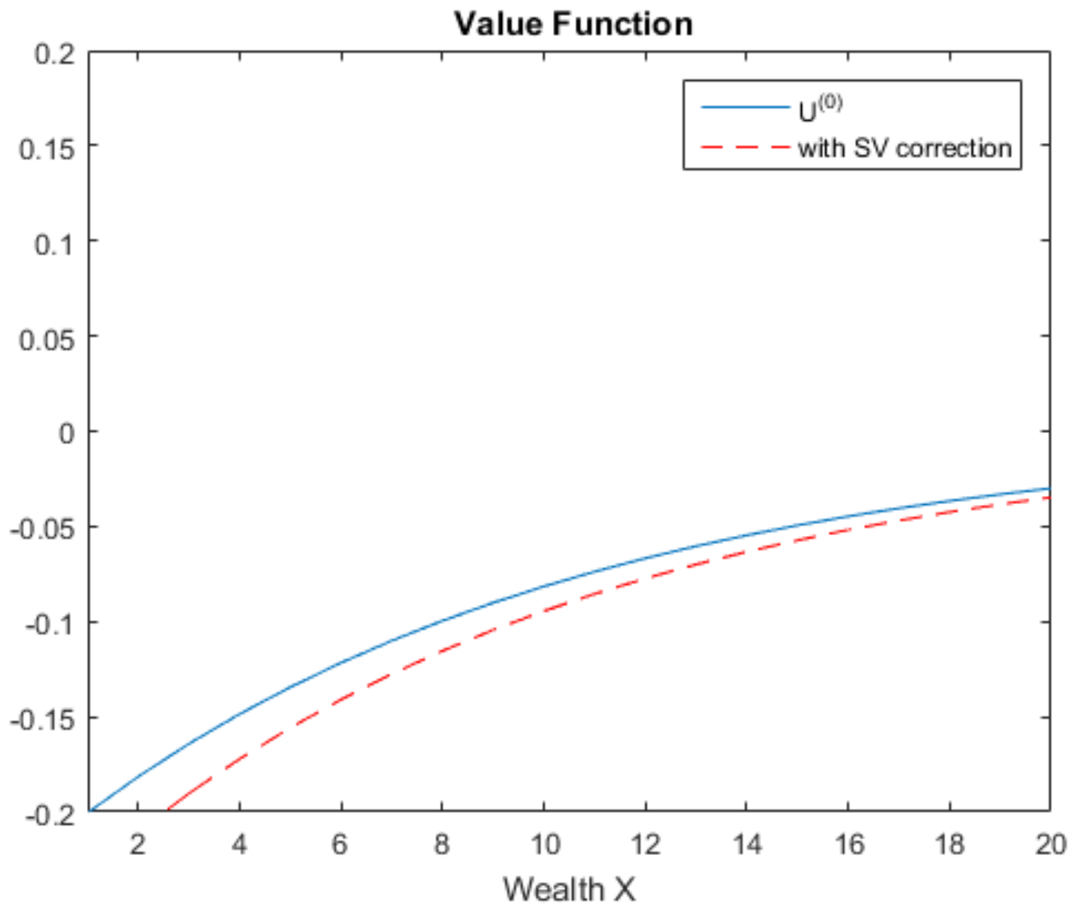
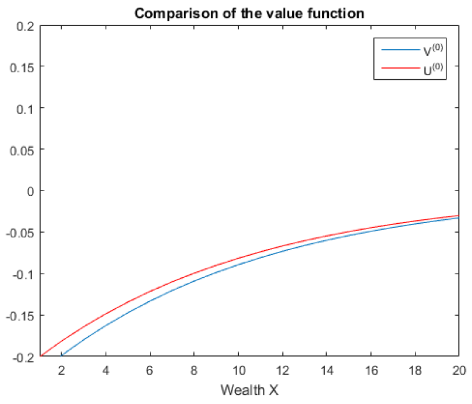
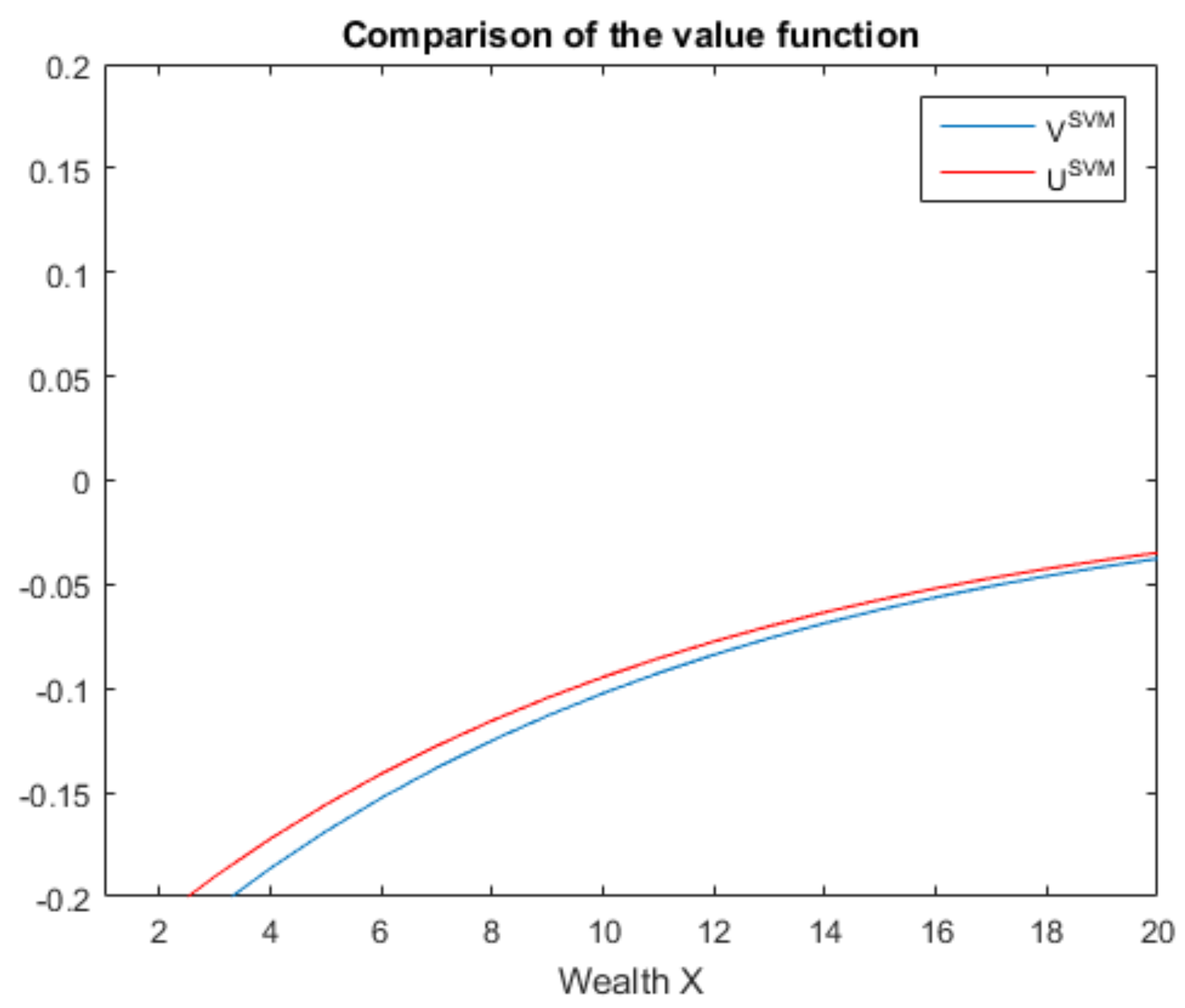
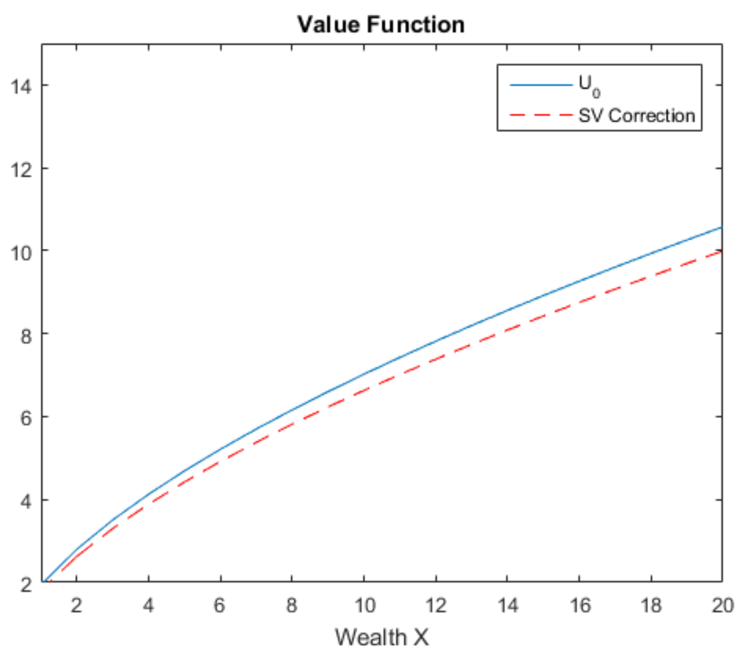
5.1. Analysis of the Value Function

The utility we use from Bond seller is exponential and is given by

$$V(x)=-e^{-\gamma x},$$

(96)

where $\gamma >0$ represents the risk aversion parameter. We can prove that the utility function is concave and increasing since

$$V^{\prime }(x)=\gamma e^{-\gamma x}>0,V^{\prime \prime }(x)=-{\gamma }^2{e}^{-\gamma x}<0.$$

(97)

The concave property of the utility function implies that the bond seller is risk aversion. The risk aversion rate is calculated by the Arrow-Pratt index,

$$AP[U]:=-\frac{U^{″}(x)}{U^{\prime }(x)}=\gamma ,$$

(98)

where the larger the $\gamma$ is, the higher risk averse the agent is. The risk-tolerance function at terminal time T is

$$R(T,x)=-\frac{U^{\prime }}{U^{″}}=\frac{1}{\gamma }.$$

(99)

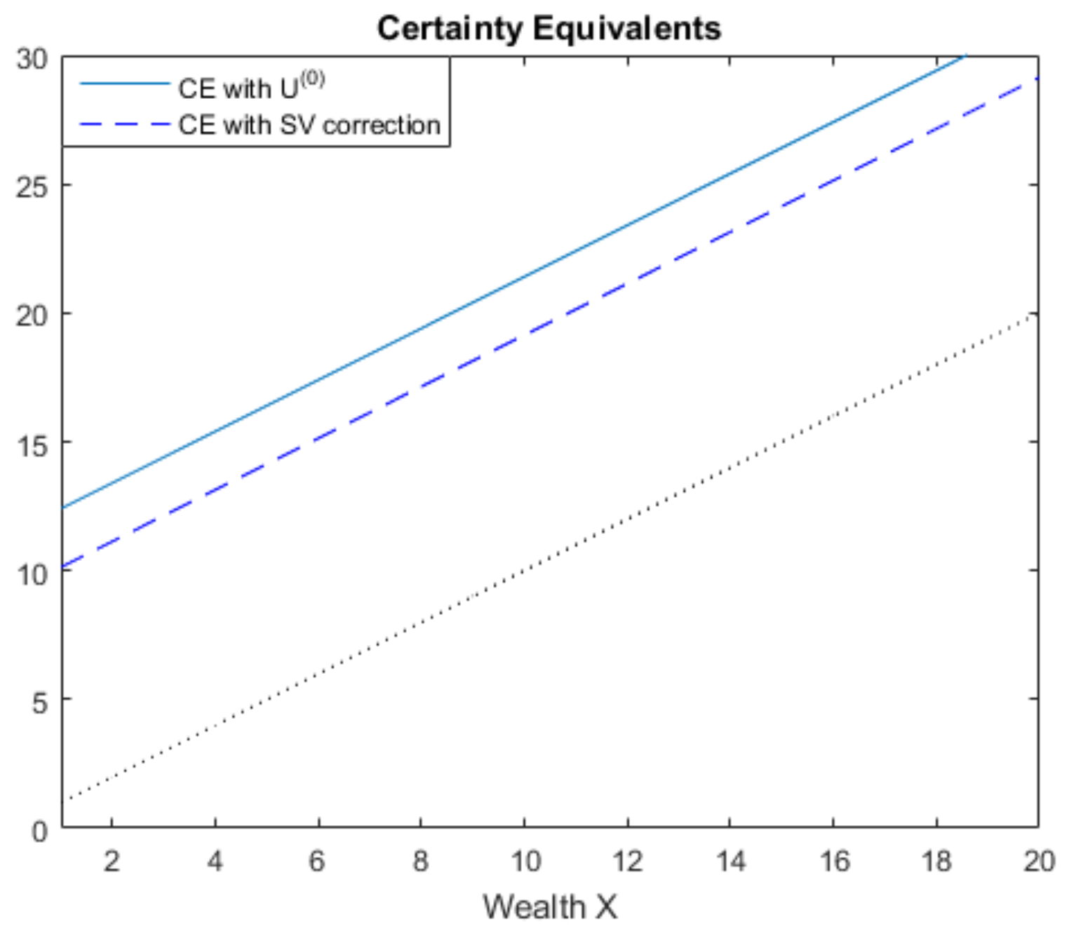
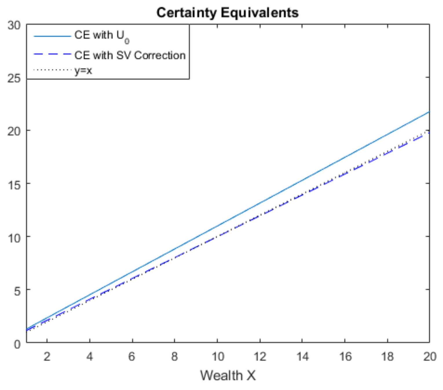
5.2. The Effect of Volatility Correction

The study above is all based on the general form. In order to demonstrate the result graphically, we give the special case as follows:

$$\begin{array}{cc}\hfill \frac{d{S}_t}{S_t}& =Y_{t}dt+\sqrt{Y_t}d{W}_t,\hfill \end{array}$$

(100)

$$\begin{array}{cc}\hfill d{Y}_t& =\frac{1}{\xi }(m_1-Y_t)dt+\sqrt{\frac{2}{\xi }}vd{W}_t^{(1)}.\hfill \end{array}$$

(101)

If $Y_t$ is an ergodic process, it has the distribution of $N(m_1,v^2)$. Assuming that $m_1=0.01$, $v^2=0.25$, $\xi =\frac{1}{200}$, and based on the definition of $\widehat{\theta }$, we obtain

$$\widehat{\theta }=\frac{1}{\sqrt{2\pi }v}{\int }_{-\infty }^{\infty }\sqrt{y}{e}^{-\frac{{(y-m_1)}^2}{2v^2}}dy$$

(102)

According to (57) and (79), we get the solution of $V^{(0)}$, and also the fast modification term of $V^{(1)}$, we then calculate the utility term as $V^{(0)}+\sqrt{\xi }{V}^{(1)}$. The approximations to the value functions are plotted in Figure 1 and Figure 2.

Also, since the bond pays $1 on maturity date T if the firm has survived till then, the bond seller’s value function will be higher than the bond holder’s value function. The comparison of the value function is shown in Figure 3 and Figure 4. The Stochastic Volatility Model(SVM) in Figure 4 represents the Stochastic Volatility(SV) modification form.

The approximate indirect utilities $V^{(0)}$ or $V^{(0)}+\sqrt{\xi }{V}^{(1)}$ can also be represented by their certainty equivalents $U^{-1}(V^{(0)})$ and $U^{-1}(V^{(0)}+\sqrt{\xi }{V}^{(1)})$, which are shown in Figure 5 and Figure 6.

In Figure 1 and Figure 2, the original value function is denoted by blue line, while the dashed blue line is the value function with stochastic volatility correction. We can see clearly that the correction line is a little lower than the original line. In Figure 3 and Figure 4, we make a comparison of the value function for holding and not holding the bond. Figure 3 shows the relationship before SV correction while Figure 4 shows the relationship after SV correction. Figure 5 and Figure 6 show the certainty equivalent before or after the correction; the solid line shows the certainty equivalent before the correction and the dashed line shows the after situation.

Therefore, we can draw the conclusion that by adding a stochastic volatility process into model (101), the investor becomes more risk adverse. The stochastic Volatility is lower than both the utility function and the certainty equivalent. Also, as bond holder will get a fixed pay at the maturity date if default does not happen, the value function of the bond holder will be a little higher than that of the bond seller. That is why we give the definition of indifference price $p_0$. By cutting down the initial wealth of bond holder, the expected utility of bond holder should be the same as that of the bond seller. In the following subsection, we will analyse the indifference and yield spread numerically.

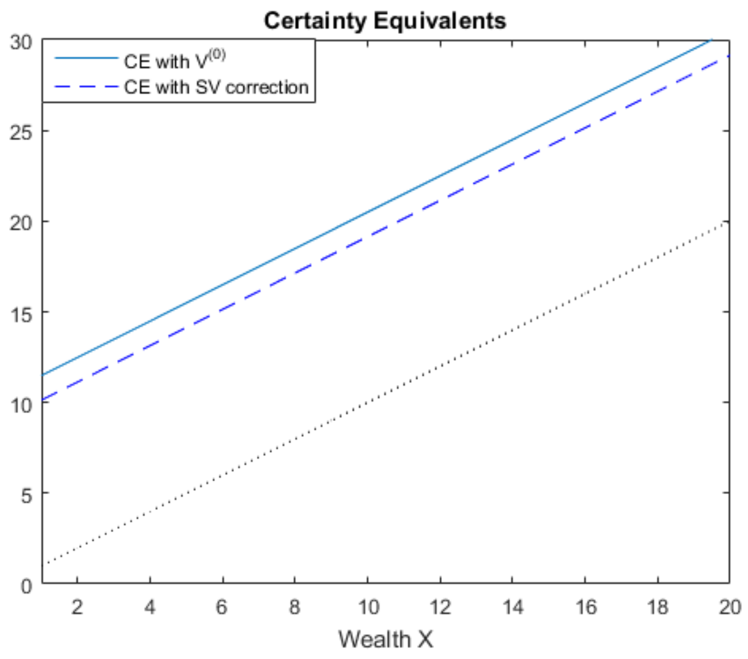
5.3. Analysis of Yield Spread

According to the Definition 1, it is easy to calculate $p_0$ and the yield spread. Without the modification term, the indifference price $p_0^{(0)}$ is given by

$$p_0^{(0)}=e^{-rT}+\frac{1}{\gamma }ln\frac{u-(1-u)e^{-(\frac{1}{2}{\widehat{\theta }}^2+\lambda )T}}{u{e}^{\gamma c}-(1-u{e}^{\gamma c})e^{-(\frac{1}{2}{\widehat{\theta }}^2+\lambda )T}},$$

(103)

where

$$u=\frac{\lambda }{\frac{1}{2}{\widehat{\theta }}^2+\lambda }.$$

(104)

If $\gamma$ takes the value of 0.05, 0.1, 0.25, 0.5 and 0.75 respectively, we obtain the profile of yield spread $y_0(T)=-\frac{1}{T}log(p_0^{(0)}(T))-r$ as shown in Figure 7.

It is noted that the yield spread is not flat even though the intensity is a constant, and this is due to the effect of the intensity rate $\lambda$ upon T. When T goes to infinity, yield spread will convergent to a long time level and become flat. As we can read from Figure 7, the yield spread for the investor is upward sloping and is approximated to a long time level due to the different maturity time.

6. Numerical Study of CRRA Utility

The utility we use from Bond seller is exponential and given by

$$V(x)=c_0\frac{x^{1-\gamma }}{1-\gamma },$$

(105)

where $\gamma >0$ represents the risk aversion parameter. We can prove that the utility function is concave and increasing since

$$V^{\prime }(x)=x^{-\gamma }>0,V^{″}(x)=-\gamma x^{-\gamma -1}<0.$$

(106)

The concave property of the utility function implies that the bond seller is risk aversion. The risk aversion rate is calculated by the Arrow-Pratt index,

$$AP[U]:=-\frac{U^{″}(x)}{U^{\prime }(x)}=\gamma /x,$$

(107)

where the larger the $\gamma$ is, the higher risk averse the agent is. And the risk-tolerance function at terminal time T is

$$R(T,x)=-\frac{U^{\prime }}{U^{″}}=\frac{1}{\gamma }x.$$

(108)

Under the assumption of the CRRA utility form, the above leading term and the first-order correction term reduce to

$$\begin{array}{ccc}\hfill V_t^{(0)}-\frac{1}{2}{\widehat{\theta }}^2\frac{{(V_x^{(0)})}^2}{V_{xx}^{(0)}}-\lambda V^{(0)}& =& -\lambda c_0\frac{x^{1-\gamma }}{1-\gamma },\hfill \end{array}$$

(109)

$$\begin{array}{ccc}\hfill V_t^{(1)}-<NL(1)>-\lambda V^{(1)}& =& 0,\hfill \end{array}$$

(110)

with the terminal condition $V^{(0)}(T,x)=c_0\frac{x^{1-\gamma }}{1-\gamma }$ and $V^{(1)}(T,x)=0$. The leading term can be solved analytically by assuming

$$V^{(0)}=x^{1-\gamma }M(t).$$

(111)

Substituting (111) into (109), we obtain the following ordinary differential equation(ODE)

$$M_t+(\frac{1-\gamma }{2}{\widehat{\theta }}^2-\lambda )M=-\frac{\lambda c_0}{1-\gamma },$$

(112)

with the terminal condition $M(T)=\frac{1}{1-\gamma }$. Solving the above ODE together with the initial condition, we obtain

$$V^{(0)}=\left(-\frac{\lambda c_0}{\lambda -\frac{1-\gamma }{2\gamma }{\widehat{\theta }}^2}+\left(\frac{1}{1-\gamma }+\frac{\lambda c_0}{\lambda -\frac{1-\gamma }{2\gamma }{\widehat{\theta }}^2}\right)e^{-(\lambda -\frac{1-\gamma }{2\gamma }{\theta }^2)(T-t)}\right)x^{1-\gamma },$$

(113)

Similarly, we solve $U_0$ with respect to the terminal condition of $U^{(0)}(T,x)={(x+c)}^{1-\gamma }/(1-\gamma )$, and obtain

$$U^{(0)}=\left(-\frac{\lambda c_0}{\lambda -\frac{1-\gamma }{2\gamma }{\widehat{\theta }}^2}+\left(\frac{1}{1-\gamma }{(\frac{x+c}{x})}^{1-\gamma }+\frac{\lambda c_0}{\lambda -\frac{1-\gamma }{2\gamma }{\widehat{\theta }}^2}\right)e^{-(\lambda -\frac{1-\gamma }{2\gamma }{\theta }^2)(T-t)}\right)x^{1-\gamma },$$

(114)

In order to obtain the first order correction term $V^{(1)}$, we assume $V^{(1)}=-(T-t)\frac{1}{2}{\rho }_{1}B{D}_1^2{V}^{(0)}(t,x+c(t,x))$, with $c(t,x)$ satisfying

$$\begin{array}{c}\hfill {\mathcal{L}†}_{t,x}c(t,x)=(T-t)\frac{1}{2}{\rho }_{1}B\lambda c_0{D}_1^2\frac{x^{1-\gamma }}{1-\gamma },c(T,x)=0.\end{array}$$

(115)

We can not derive the analytic form of the solution of the above equation because the right hand side of the equation is not necessary an affine structure. In this case, we solve it numerically by finite element discretization shown in Appendix A.

The results are shown in Figure 8 and Figure 9, from which we know that value function is concave and increasing considering the risk attitude. However, the fast scale stochastic volatility correction drag the value function a little bit downward, and the main reason is that incorporation of uncertain volatility gives the investors more risk exposure.

Similar results are also shown in the certainty equivalents, that is incorporation of stochastic volatility lower down the value function, as shown in Figure 10 and Figure 11.

Table 1. Sensitivity study of parameters.

Name	Value	Sensitivity
$m1$	0.11	3.65%
v	0.25	1.80%
$\lambda$	0.5	1.32%
$\rho$	0.5	−19.61%

gives the results of the percentage change of the mean value when the model parameter is given a $1\%$ change. Clearly, the value function is sensitive to the correlation rate, and the long term mean variance $m1$ is more sensitive compared to the volatility of volatility.

7. Conclusions and Future Work

In this paper, we study the single-name bond under the stochastic intensity and the stochastic volatility. In order to solve the non-linear PDE, we use the method of asymptotic approximation. We establish the expression of leading term $V^{(0)}$, and fast-scale modification term $V^{(1)}$. By comparing the leading term and the utility with fast scale modification, we can draw the conclusion that by considering the effects of the fast-scale volatility, investors become more and more risk aversive, which lowers down their utility and increases the certainty equivalents. Also, according to the analysis above, we prove that the yield spread of the investor goes up with the maturity time and converges to a long time level. The advantage of the asymptotic method is that it reduces the high dimensional problem into a lower dimensional problem, which is relatively easy to solve. However, the limitation of this approach is that it only works for a specific utility model, and for other utilities, the analytic solutions may not be obtained so that numerical method is needed. In our future research, the effect of multiscale volatility and stochastic interest rate will be taken into consideration.

References

1. Tan, Y.; Floros, C. Risk, capital and efficiency in Chinese banking. J. Int. Financ. Mark. Inst. Money 2013, 26, 378–393. [Google Scholar] [CrossRef] [Green Version]
2. Tan, Y. The impacts of risk and competition on bank profitability in China. J. Int. Financ. Mark. Inst. Money 2016, 40, 85–110. [Google Scholar] [CrossRef]
3. Madan, D.B.; Unal, H. Pricing the risks of default. Rev. Deriv. Res. 1998, 2, 121–160. [Google Scholar] [CrossRef]
4. Jarrow, R.A.; Turnbull, S.M. Pricing derivatives on financial securities subject to credit risk. J. Financ. 1995, 50, 53–85. [Google Scholar] [CrossRef]
5. Lando, D. On Cox processes and credit risky securities. Rev. Deriv. Res. 1998, 2, 99–120. [Google Scholar] [CrossRef]
6. Hao, C.; Zhang, B.; Carling, K.; Alam, M.M. Review of the Literature on Credit Risk Modeling: Development of the Recent 10 Years; Business Perspectives: Sumy, Ukraine, 2009. [Google Scholar]
7. Black, F.; Scholes, M. The pricing of options and corporate liabilities. J. Political Econ. 1973, 81, 637–654. [Google Scholar] [CrossRef]
8. Sircar, R.; Zariphopoulou, T. Utility valuation of credit derivatives: Single and two-name cases. Adv. Math. Financ. 2007, 279–301. [Google Scholar] [CrossRef]
9. Papageorgiou, E.; Sircar, R. Multiscale intensity models for single name credit derivatives. Appl. Math. Financ. 2008, 15, 73–105. [Google Scholar] [CrossRef]
10. Merton, R.C. Optimum consumption and portfolio rules in a continuous-time model. J. Econ. Theory 1971, 3, 373–413. [Google Scholar] [CrossRef]
11. Heston, S.L. A closed-form solution for options with stochastic volatility with applications to bond and currency options. Rev. Financ. Stud. 1993, 6, 327–343. [Google Scholar] [CrossRef]
12. Longstaff, F.A.; Schwartz, E.S. A simple approach to valuing risky fixed and floating rate debt. J. Financ. 1995, 50, 789–819. [Google Scholar] [CrossRef]
13. Fouque, J.P.; Papanicolaou, G.; Sircar, R.; Solna, K. Multiscale stochastic volatility asymptotics. Multiscale Model. Simul. 2003, 2, 22–42. [Google Scholar] [CrossRef]
14. Fouque, J.P.; Sircar, R.; Zariphopoulou, T. Portfolio optimization and stochastic volatility asymptotics. Math. Financ. 2017, 27, 704–745. [Google Scholar] [CrossRef]
15. Hodges, S.D.; Neuberger, A. Optimal Replication of Contingent Claims under Transaction Costs. Rev. Futures Mark. 1989, 8, 222–239. [Google Scholar]
16. Davis, M.; Yoshikawa, D. An equilibrium approach to indifference pricing. Adv. Financ. Eng. 2012, 29–56. [Google Scholar] [CrossRef]
17. Fouque, J.P.; Papanicolaou, G.; Sircar, R.; Solna, K. Multiscale Stochastic Volatility for Equity, Interest Rate, and Credit Derivatives; Cambridge University Press: Cambridge, UK, 2011. [Google Scholar]
18. Duffie, D.; Zariphopoulou, T. Optimal investment with undiversifiable income risk. Math. Financ. 1993, 3, 135–148. [Google Scholar] [CrossRef]
19. Sircar, R.; Zariphopoulou, T. Utility valuation of multi-name credit derivatives and application to CDOs. Quant. Financ. 2010, 10, 195–208. [Google Scholar] [CrossRef]
20. Brémand, P. Point Processes and Queues; Springer: New York, NY, USA, 1981. [Google Scholar]
Figure 1. Value Function of Bond Seller.
Sustainability 10 01027 g001
Figure 2. Value Function of Bond Holder.
Sustainability 10 01027 g002
Figure 3. Leading Term Value Function.
Sustainability 10 01027 g003
Figure 4. SV Modification Value Function.
Sustainability 10 01027 g004
Figure 5. Certainty Equivalents of Bond Seller.
Sustainability 10 01027 g005
Figure 6. Certainty Equivalents of Bond Holder.
Sustainability 10 01027 g006
Figure 7. Yield Spread.
Sustainability 10 01027 g007
Figure 8. Value Function of Bond Seller.
Sustainability 10 01027 g008
Figure 9. Value Function of Bond Holder.
Sustainability 10 01027 g009
Figure 10. Certainty Equivalents of Bond Seller.
Sustainability 10 01027 g010
Figure 11. Certainty Equivalents of Bond Holder.
Sustainability 10 01027 g011