Dependence Structures and Systemic Risk of Government Securities Markets in Central and Eastern Europe: A CoVaR-Copula Approach

Abstract

In this study, we proposed a new empirical method by combining generalized autoregressive score functions and a copula model with high-frequency data to model the conditional time-varying joint distribution of the government bond yields between Poland/Czech Republic/Hungary, and Germany. Capturing the conditional time-varying joint distribution of these bond yields allowed us to precisely measure the dependence of the government securities markets. In particular, we found a high dependence of these government securities markets in the long term, but a low dependence in the short term. In addition, we report that the Czech Republic showed the highest dependence with Germany, while Hungary showed the lowest. Moreover, we found that the systemic risk dynamics were consistent with the idea that the global financial crisis not only had spillover effects on countries with weak economic fundamentals (e.g., Hungary, which had the highest systemic risk), but also had contagion effects for both CEEC-3 countries and Germany. Finally, we confirm that three major market events, namely the EU accession, the global financial crisis, and the European debt crisis, caused structural changes to the dynamic correlation.

1. Introduction

Measuring the dependence structures of government securities markets is garnering considerable attention from academia as well as from financial institutions, given the continuing expansion of the European Union (EU). In 2004, 10 countries from Central and Eastern Europe and the Mediterranean region joined the EU, which served as a historic step towards unifying Europe after several decades of division that had resulted from the Cold War. In this study, rather than investigating correlations, we propose a new approach to investigate the dependence structures among these countries’ financial markets including the investigation of general correlations as well as tail correlation.

Financial markets become integrated when economies strongly depend on one other. This process not only reduces transaction costs, but also improves the efficiency of information sharing. However, although financial integration increases overall market efficiency, it reduces the diversification benefits available to prospective investors. Thus, investigating the dynamic process of financial integration allows us not only to measure the interdependence of economies, but also to provide useful information for investors.

Here, we propose a new method for evaluating the degree to which the integration processes and risk spillovers in Central and Eastern Europe have evolved over time. To simplify our analysis, we chose Poland, the Czech Republic, and Hungary (termed as the CEEC (Central and Eastern European countries)-3 hereafter) to represent Central and Eastern Europe given that these countries have the largest economies and financial markets in the region as well as the best data availability. To represent the EU, we chose Germany because of its economic background and geographic factors. Therefore, we investigated the differences in the dependence structures of the government securities markets in the CEEC-3 and Germany.

Two types of approaches tend to be used to study dependence structures. The first type includes observation-based methods such as those based on the generalized autoregressive conditional heteroskedasticity (GARCH) framework [1,2]. The dynamic conditional correlation (DCC-GARCH)-based approach [3,4,5] and copula-GARCH-based approach [6,7,8] are representative examples. The second type is parameter-based methods. The classical analysis of this type focuses on time-varying parameters, which allows us to better characterize the dynamic correlations in government securities markets by using easy estimations. For example, Pozzi and Wolswijk [9] employed a linear state space approach to estimate the latent factor decomposition of the excess returns or risk premiums suggested by a standard international capital asset pricing model for government bonds. They found that the government bond markets in the Eurozone under investigation were almost fully integrated by the end of 2006, showing that an important part of the achieved convergence was reversed during 2007–2009. Bekiros [10] also provided evidence that time-varying parameter models more accurately forecast Eurozone economies than other models.

In this study, we employed a parameter-driven model, namely the generalized autoregressive score (GAS) model, to investigate the dynamic integrated process of European government securities markets. For example, Creal et al. [11] employed the GAS model to analyze the dynamic correlation between the euro and yen, and between the euro and pound. Meanwhile, Oh and Patton [12] and Creal and Tsey [13] provided evidence that the GAS model could be employed with high dimensional copula to investigate the interdependence among different assets. With regard to the topics of the present study, Boubakri and Guillaumin [14] provided evidence that financial integration was not perfect, but was increasing based on the dynamic correlation of the foreign exchange rate. Furthermore, they also showed that financial contagion occurred during the global financial crisis.

Instead of focusing on the foreign exchange rate, in this study, we investigated the integration of these countries based on interest rates (e.g., bond yields). Moreover, in contrast to the studies of Yang and Hamori [5,7,8] who focused on investigating observations, we computed time-varying parameters. The technique adopted herein was based on the score function of the predictive model density at time t by incorporating the non-linear property. In addition, in contrast to observation-driven models, the GAS model has the advantage of exploiting the complete density structure rather than only means and higher moments. Furthermore, its applications can be extended to asymmetric, long memory, and other more complicated dynamics without increasing model complexity. Therefore, by employing the GAS framework, we restructured the time-varying copula model to investigate the dynamic integrations of the government securities markets in Eastern Europe.

To understand the risk spillover effect between the CEEC-3 and Germany, we employed copulas to compute the conditional value-at-risk (CoVaR) by providing quantitative evidence on the systemic risk spillovers in government securities markets. Furthermore, we evaluated how the deteriorating financial position of a sovereign market could impair the performance of other government securities markets during a crisis. In particular, we used the CoVaR measures originally proposed by Adrian and Brunnermeier [15] and generalized by Girardi and Ergün [16], which allowed us to capture the possible risk spillovers between markets by providing information on the value-at-risk (VaR) of a market, conditional on the fact that another market is in financial distress.

By adopting a two-step procedure, we easily obtained the value of the CoVaR. In the first step, we computed the cumulative probability of the CoVaR from a copula function by assuming the cumulative probability of the VaR of the market in financial distress, and the confidence level of the CoVaR. In the second step, we obtained the value of the CoVaR by inverting the marginal distribution function for this cumulative probability. Moreover, by employing GAS specifications, we obtained more sensitive information on the risk spillover effect in the government securities markets of the CEEC-3 and Germany.

Our contributions to the body of knowledge are threefold. First, we provide more specific details on the dependence across different maturities when compared with previous studies. Second, we implemented a new approach (i.e., the GAS-based dynamic Gaussian copula) to investigate the dynamic correlations among these markets, which can provide us with more sensitive correlations to the structural changes. This approach allowed us to analyze how the degree of dependence changed according to major market events, namely the EU accession (2004), the global financial crisis (2008), and the European debt crisis (2012). Third, we compared and contrasted the risk spillover effect in the government securities markets of the CEEC-3 and Germany by employing both the Gaussian copula model and the Gaussian copula GAS model. Finally, we employed the Symmetrized Joe-Clayton copula (SJC copula; [17]) to investigate the tail dependence of these markets and compared them with the results from the GAS-based model to verify the robustness of the results.

The remainder of this article is organized as follows. Section 2 discusses the copulas and verifies the time-varying dependence structure. Section 3 describes the data and statistical issues. Section 4 provides the empirical results and Section 5 concludes.

2. Method

In this section, we first describe the margins of the return distributions based on our empirical model. Second, we introduce the specifications of the dynamic copula model. Then, we selected one particular elliptical copula (Gaussian copula) model to investigate the dependence of the government securities markets in Eastern Europe. Furthermore, we estimated the systemic risk of these countries based on both the Gaussian copula and the Gaussian copula GAS models. Finally, to justify the empirical findings, we employed the SJC copula to examine the dynamic tail dependence of the examined government securities markets.

2.1. Marginal Distribution Specifications

The marginal distribution for each return series is characterized by a Glosten-Jagannathan-Runkle GARCH (GJR-AR(k)-GARCH(1,1)-Skew-t; [18]) model that considers the effects of asymmetric information [18,19,20]. Assume $R_{i,t}$ and $h_{i,t}$ to be bond i’s return and conditional variance for period t, respectively. Thus, the GJR-AR(k)-GARCH(1,1)-Skew-t model for the bond return is

$$R_{it}={\mu }_i+{\alpha }_{i,1}{R}_{i,t-1}+{\alpha }_{i,2}{R}_{i,t-2}+\cdots +{\alpha }_{i,k}{R}_{i,t-k}+{\epsilon }_{i,t}$$

(1)

$$h_{i,t}={\omega }_i+{\beta }_i{h}_{i,t-1}+{\delta }_i{\epsilon }_{i,t-1}^2+\cdots +{\gamma }_i{s}_{i,t-1}{\epsilon }_{i,t-1}^2$$

(2)

where $s_{i,t-1}=1$ when ${\epsilon }_{i,t-1}$ is negative and $s_{i,t-1}=0$ otherwise. We assumed that the error term ${\epsilon }_{i,t}$ followed the skew-t distribution with the density function $f\left({\upsilon }_t,{\lambda }_t\right)$, such that

$$f\left(y_t;{\upsilon }_t,{\lambda }_t\right)=\{\begin{array}{c}bc{\left(1+\frac{1}{{\upsilon }_t}{\left(\frac{b{y}_t+a}{1-{\lambda }_t}\right)}^2\right)}^{-\frac{{\upsilon }_t+1}{2}}for{y}_t\le -\frac{a}{b}\\ bc{\left(1+\frac{1}{{\upsilon }_t}{\left(\frac{b{y}_t+a}{1+{\lambda }_t}\right)}^2\right)}^{-\frac{{\upsilon }_t+1}{2}}for{y}_t>-\frac{a}{b}\end{array}$$

(3)

where $c=\frac{\Gamma (\frac{{\upsilon }_t+1}{2})}{\Gamma (\frac{{\upsilon }_t}{2}\sqrt{\pi ({\upsilon }_t-2)})}$, $b=\sqrt{1+3{\lambda }_t^2-a^2}$, and $a=4{\lambda }_{t}c(\frac{{\upsilon }_t-2}{{\upsilon }_t-1})$. This density is defined for $2<{\upsilon }_t<\infty$ and $-1<{\lambda }_t<1$ [21]. For the GJR (1, 1) model, the constraints applied to Equation (3) are $\delta +\beta +2\gamma <2$, $\mathsf{\delta }>-\mathsf{\gamma }$, and $\beta \in (0,1)$, and we chose k based on the Akaike information criterion (AIC) [22].

2.2. A Copula with GAS Dynamics

After determining the suitable marginal distribution, we proceeded to the copula function. A dynamic copula model is typically used to model the dependence of government securities markets in Eastern Europe in a dynamic process. However, an important contribution of our research was to calculate the time-varying correlations between the CEEC-3 and Germany. Two types of specifications allow the parameters to vary over time. First, studies of copula-based analysis such as Hafner and Manner [23] and Manner and Segers [24] have proposed a stochastic copula model that allows the parameters to evolve as a latent time series. Second, ARCH (autoregressive conditional heteroskedasticity)-type models such as dynamic conditional correlation (DCC) [3] and their related models for copulas [11,17] permit the time-varying parameters to vary according to the functions of the lagged observables. One advantage of the second approach is that it avoids the need to “integrate out” the innovation terms driving the latent time series processes [25,26]. In addition, as pointed out by McAleer [27], DCC may suffer from the problem of the derivation of asymptotic properties of the Quasi-Maximum Likelihood Estimators. Therefore, based on the parameter-driven methodology, the Generalized Autoregressive Score (GAS) model provided us with another view of the conditional correction model as well as the CoVaR approach.

As our empirical model, we employed the GAS model of Creal et al. [11]. This function describes the time-varying copula parameter $\left({\delta }_t\right)$ as a combination of the lagged copula parameter and a forcing variable related to the standardized score of the copula log-likelihood. Following Creal et al. [11], a copula with GAS dynamics can be expressed as

$${\mathit{U}}_{\mathit{t}}|{ℱ}_{t-1}~{\mathit{C}}_{\mathit{t}}\left({\delta }_t\left(\gamma \right)\right)$$

(4)

where $\gamma$ is the copula function’s parameter; and ${\mathit{U}}_{\mathit{t}}={\left[U_{1t},U_{2t}\right]}^{\prime }$ is the vector of the marginal conditional probability integral transform. To ensure that the correlation of the normal copula falls between the values of −1 and 1, Creal et al. [11] suggested transforming the copula parameter by using an increasing invertible function (e.g., logarithmic, logistic) to the parameter:

$${\kappa }_t=h\left({\delta }_t\right)⟺{\delta }_t=h^{-1}\left({\kappa }_t\right)$$

(5)

For a copula with a transformed time-varying parameter ${\delta }_t$, a GAS (1,1) model can be described as

$${\kappa }_{t+1}=\omega +b{\kappa }_t+a{I}_t^{-\frac{1}{2}}h\left({\delta }_t\right){\mathit{s}}_{\mathit{t}}$$

(6)

$${\mathit{s}}_{\mathit{t}}\equiv \frac{\partial log\left(u_y;{\delta }_t\right)}{\partial {\delta }_t}$$

(7)

$$I_t\equiv E_{t-1}\left[{\mathit{s}}_{\mathit{t}}{\mathit{s}}_{\mathit{t}}^{\mathit{\prime }}\right]=I\left({\delta }_t\right)$$

(8)

Although the functions for the time-varying parameters are arbitrary, they can nest a variety of popular approaches from conditional variance models to trade duration and count models. Nonetheless, in contrast to the approach taken by Patton [17], GAS models are more sensitive to correlation shocks (for a comparison of the two models, see [11]).

Since we examined the dynamic process of the dependence of the government securities markets in the CEEC-3 and Germany, we employed the time-varying Gaussian copula. The conditional Gaussian copula function is defined as the density of the joint standard uniform variables $\left(u_t,v_t\right)$ with a time-varying correlation ${\rho }_t$. Moreover, we assumed that $x_t={\varphi }^{-1}\left(u_t\right)$ and $y_t={\varphi }^{-1}\left(v_t\right)$, where ${\varphi }^{-1}(·)$ represents the inverse of the cumulative density function of the standard normal distribution. Then, the density of the time-varying Gaussian copula is expressed as

$$C_t^{Gau}\left(u_t,v_t|{\rho }_t\right)=\frac{1}{\sqrt{1-{\rho }_t^2}}exp\left(\frac{x_t^2+y_t^2}{2}-\frac{x_t^2-2\rho x_t{y}_t+y_t^2}{2\left(1-{\rho }_t^2\right)}\right)$$

(9)

Thus, by combining Equation (6) with Equation (9), the Gaussian correlation parameter ${\rho }_t$ is modeled by the transformed parameter ${\rho }_t=(1-exp(-{\kappa }_t))/(1+exp(-{\kappa }_t))$, and the additional scaling factor ${\delta }_t=2/(1-{\rho }_t^2)$ in Equation (6) is the consequence of modeling the transformed correlation parameter ${\kappa }_t$ rather than ${\rho }_t$ directly. Hence, we compared and contrasted the GAS Gaussian copula estimation across maturities.

2.3. CoVaR

In this section, we quantified the VaR (Value at Risk) and CoVaR (Conditional Value at Risk) for the government securities markets in the CEEC-3 and Germany. Given the strong linkages of these markets [7], we considered the impact of financial distress in the German market (as measured by its VaR) on the VaR of the CEEC-3 market and vice versa. Following the studies of Adrian and Brunnermeier [15] and Girardi and Ergün [16], the CoVaR for asset i is the VaR for asset i conditional on the fact that asset j exhibits an extreme movement.

Let $r_t^c$ be the returns for the CEEC-3 government securities market and $r_t^d$ be the returns for the German government securities market. The downside CoVaR for stock returns for an extreme downward oil movement and a confidence level $1-\beta$ can be formally expressed as the $\beta$-quantile of the conditional distribution of $r_t^c$ as

$$Pr\left(r_t^c\le CoVa{R}_{\beta ,t}^c\left(q,p\right)|r_t^d\le Va{R}_{\alpha ,t}^d\right)=\beta$$

(10)

where $Va{R}_{\alpha ,t}^d$ is the $\alpha$-quantile of the German government securities market return distribution and $Pr\left(r_t^d\le Va{R}_{\alpha ,t}^d\right)=\alpha$ measures the maximum loss that the German government securities market returns may experience for a confidence level $1-\alpha$ and a specific time horizon.

Moreover, we measured the systemic impact of the CEEC-3 government securities market on the German government securities market by considering the CoVaR for the latter instead of the former as in Equation (10). The CoVaR in those equations can be represented in terms of copulas, since the conditional probabilities can be rewritten, respectively, as

$$C\left(F_{r_t^c}\left(CoVa{R}_{\beta ,t}^c\right),F_{r_t^d}\left(Va{R}_{\alpha ,t}^d\right)\right)=\alpha \beta$$

(11)

where $F_{r_t^c}$ and $F_{r_t^d}$ are the marginal distributions of the CEEC-3 government securities market and German government securities market returns, respectively. We followed Reboredo and Ugolini [25] in computing the CoVaR by following a two-step procedure. Following the studies of Adrian and Brunnermeier [15] and Girardi and Ergün [16], the systemic risk contribution of market j as the delta CoVaR ($∆CoVaR$) can be defined as the difference between the VaR of the overall German government securities market conditional on the distressed state of the CEEC-3 government securities market $\left(R_t^c\le Va{R}_{\alpha ,t}^c\right)$. The VaR of each of the individual CEEC-3 government securities markets can then be treated as a whole conditional on the benchmark state of the market, considering it to be the median of the return distribution of the market, or, alternatively, the VaR for α = 0.5. The systemic risk contribution of the market for each CEEC-3 country is the government securities market thus defined as

$$∆CoVa{R}_t^{c/d}=\frac{CoVa{R}_{\beta ,t}^{c/d}-CoVa{R}_{\beta ,t}^{c/d,\alpha =0.5}}{CoVa{R}_{\beta ,t}^{d,\alpha =0.5}}$$

(12)

The primary shortcoming of such a specification is that it estimates the contemporaneous correlation with the market to gauge the size of the potential tail spillover effects. In other words, it is useful as it captures the marginal contribution of markets to the overall systemic risk. In this study, we investigated the risk spillover effects between the CEEC-3 countries and Germany by employing both the Gaussian copula model and Gaussian copula GAS model.

2.4. Estimation Method

In the final step, we employed the multi-stage maximum likelihood (MSML) estimation method to calculate the dynamic relationships between the government securities markets in the CEEC-3 and Germany. First, we estimated the marginal distributions separately. In the second step, we estimated the copula model conditioned on the estimated marginal distribution parameters. Therefore, the final dynamic copula with the GAS process based on the GARCH model can be specified as

$$\begin{gathered} ℒ\left(\theta \right)={{\displaystyle \sum }}_{i=1}^{T}log\left({\mathit{f}}_{\mathit{t}}\left({\mathit{X}}_{\mathit{t}};\theta \right)\right)={{\displaystyle \sum }}_{i=1}^T\log \left(f_{1t}\left(X_{1,t};{\theta }_1\right)\right)+{{\displaystyle \sum }}_{i=1}^T\log \left(f_{2t}\left(X_{2,t};{\theta }_2\right)\right) \\ +{{\displaystyle \sum }}_{i=1}^T\log \left({\mathit{c}}_{\mathit{t}}\left(F_{1,t}\left(X_{1,t};\theta \right),F_{2,t}\left(X_{2,t};{\theta }_c\right)\right)\right) \end{gathered}$$

(13)

where $\theta ={\left({\varphi }^{\prime },{\gamma }^{\prime }\right)}^{\prime }$ is the estimated vector of all the parameters including those of the marginal distributions $\varphi$ and of the copula $\gamma$.

3. Data

To investigate the dependence of the CEEC-3 and Germany across maturities, we employed 3-month, 1-year, 3-year, 5-year, and 10-year government bond yields based on a daily frequency. In particular, we focused on 3-year, 5-year, and 10-year government bond yields and omitted 3-month and 1-year government bond yields due to the availability of data and empirical results. For instance, the short-term interest rate for 3-month and 1-year yields cannot model the stable dynamic correlation between Hungary and Germany since the estimation procedure does not converge. Thus, the data on 3-month and 1-year yields did not fit the model well as there were too many poorly fitting observations. Moreover, the marginal distribution for Poland was not well specified since the GARCH process was hardly justified.

The sample period ran from 1 January 2002 to 31 December 2016. The total dataset was comprised of 3914 valid observations. In all cases, bond returns were calculated as the first differences of the logs of yields.

Table 1. Summary statistics across different maturities.

	Poland	Hungary	Czech Republic	Germany
3-year
Mean	–0.000366	−0.000562	−0.000653	−0.000225
Std. Dev.	0.016497	0.017400	0.140969	0.167249
Skewness	0.678808	1.424991	−0.416608	0.682362
Kurtosis	11.01275	22.50707	87.16472	65.51154
JB	10,771.20 ***	63,382.03 ***	1,145,605 ***	628,135.2 ***
Observations	3914	3914	3914	3914
5-year
Mean	−0.000303	−0.000380	−0.000874	−0.000848
Std. Dev.	0.015542	0.017361	0.169736	0.165198
Skewness	0.447378	0.761848	1.162340	2.072385
Kurtosis	13.77973	15.21576	188.6507	218.0410
JB	19,081.27 ***	24,714.69 ***	5,574,346 ***	7,432,406 ***
Observations	3914	3914	3914	3914
10-year
Mean	−0.000225	−0.000204	−0.000636	0.000268
Std. Dev.	0.013174	0.015519	0.022779	0.124821
Skewness	0.496346	0.154218	0.336106	−0.555559
Kurtosis	13.80813	10.68544	28.27690	206.1039
JB	19,211.42 ***	9648.186 ***	103,392 ***	6,627,889 ***
Observations	3914	3914	3914	3914

Notes: *, **, and *** represent significance at the 10%, 5%, and 1% levels, respectively.

reports the descriptive statistics of the return series. Particularly, we witnessed the increasing of interest rate for the CEEC-3 countries across the different term structures during our sample periods. In addition, the negative returns of the bond yields also indicated the bad credit environment in the CEEC-3 countries where investors require higher nominal interests. The reason may be due to the saving-investment imbalance with other developed countries such as Germany, whose mean return for ten-year bond yield was still positive. Compared to Germany, the CEEC-3 countries have to deal with their debt problem. For example, the government of Hungary faces a great fiscal deficit and struggles to solve its debt problem. The results of the Jarque–Bera (JB) test showed that the null hypothesis of the normal distribution was rejected in all cases.

4. Empirical Results

4.1. Marginal Distribution Estimations

In the first step, we employed univariate GJR-AR(k)-GARCH(1,1)-Skew-t models to model the marginal distributions. Based on the SBIC (Schwarz Bayesian information criterion) [28], we selected k = 2 for the 3-year maturity and k = 1 for the 5-year and 10-year maturities.

Table 2. Estimation results of the marginal distribution for 3-year yields.

	Poland	Hungary	Czech Republic	Germany
Mean Equation
μ1 × 10−4	−5.211 (2.115) ***	−4.897 (2.511) **	−0.788 (0.745)	1.388 (1.546)
α	−0.024 (0.015)	−0.018 (0.015)	−0.051 (0.015) ***	−0.029 (0.023)
Variance Equation
ω × 10−5	3.414 (1.125) ***	2.251 (2.332)	3.112 (1.052) ***	1.718 (0.344)
δ	0.108 (0.053) ***	0.149 (0.607) ***	0.249 (0.075) ***	0.206 (0.051) ***
β	0.805 (0.039) ***	0.716 (0.101) ***	0.753 (0.038) ***	0.772 (0.031) ***
γ	0.023 (0.039)	−0.129 (0.365)	0.213 (0.065) ***	0.250 (0.012) ***
υ	3.138 (0.209) ***	2.492 (0.416) ***	2.646 (0.106) ***	3.384 (0.581) ***
λ	0.023 (0.018)	0.014 (0.016)	0.048 (0.015) ***	0.049 (0.025) *
Diagnostic
Q(20)	23.21 [0.588]	36.54 [0.251]	81.22 [0.245]	21.18 [0.227]
Q2(20)	13.23 [0.786]	21.55 [0.127]	44.87 [0.621]	17.97 [0.419]
Log-Likelihood	11,202.57	10,244.36	8596.28	8496.57

Notes: The numbers in parentheses are standard errors. The numbers in square brackets are p-values. Q(20) (Q²(20)) is the Ljung–Box Q statistic for the null hypothesis that there is no autocorrelation up to order 20 for the standardized residuals (standardized squared residuals). *, **, and *** represent significance at the 10%, 5%, and 1% levels, respectively.

,

Table 3. Estimation results of the marginal distribution for 5-year yields.

	Poland	Hungary	Czech Republic	Germany
Mean Equation
μ1 × 10−4	−2.618 (2.110)	5.124 (2.221) **	−5.428 (4.775)	3.781 (1.546) ***
α	−0.008 (0.019)	0.031 (0.015) **	−0.086 (0.017) ***	0.332 (0.015) ***
Variance Equation
ω × 10−5	2.414 (3.125)	4.141 (1.128)	1.787 (1.188)	1.221 (1.188)
δ	0.091 (0.037) ***	0.154 (0.013) ***	0.073 (0.001) ***	0.012 (0.002) ***
β	0.911 (0.028) ***	0.842 (0.039) ***	0.891 (0.028) ***	0.944 (0.015) ***
γ	0.008 (0.028)	0.139 (0.005)	0.145 (0.016) ***	0.099 (0.005) ***
υ	3.806 (0.281) ***	2.445 (0.055) ***	2.836 (0.588) ***	7.367 (0.568) ***
λ	0.013 (0.053)	0.015 (0.016)	0.027 (0.021)	0.071 (0.101)
Diagnostic
Q(20)	15.21 [0.448]	41.27 [0.651]	82.12 [0.245]	22.54[0.347]
Q2(20)	3.286 [1.000]	14.22 [0.234]	44.11 [0.621]	14.27 [0.721]
Log-Likelihood	11,235.812	10,113.699	10,244.87	9853.126

Notes: The numbers in parentheses are standard errors. The numbers in square brackets are p-values. Q(20) (Q²(20)) is the Ljung–Box Q statistic for the null hypothesis that there is no autocorrelation up to order 20 for the standardized residuals (standardized squared residuals). *, **, and *** represent significance at the 10%, 5%, and 1% levels, respectively.

and

Table 4. Estimation results of the marginal distribution for 10-year yields.

	Poland	Hungary	Czech Republic	Germany
Mean Equation
μ1 × 10−4	2.568 (0.221) ***	6.351 (1.121) ***	−4.298 (1.125) ***	2.121 (0.285) ***
α	−0.042 (0.011)	0.046 (0.031)	−0.009 (0.018)	0.089 (0.119)
Variance Equation
ω × 10−5	3.122 (1.155) ***	2.886 (1.085) ***	1.987 (0.788) ***	4.221 (1.688) ***
δ	0.116 (0.032) ***	0.111 (0.003) ***	0.166 (0.078) ***	0.017 (0.007) ***
β	0.891 (0.025) ***	0.832 (0.054) ***	0.835 (0.053) ***	0.961 (0.006) ***
γ	−0.023 (0.021)	0.024 (0.469)	0.046 (0.041)	0.041 (0.009) ***
υ	4.012 (0.324) ***	2.319 (0.607) ***	2.996 (0.256) ***	11.621 (2.152) ***
λ	0.009 (0.012)	−0.055 (0.019)	0.015 (0.017)	0.026 (0.022)
Diagnostic
Q(20)	15.26 [0.541]	69.17 [0.265]	55.32 [0.185]	12.96 [0.899]
Q2(20)	1.565 [1.000]	24.75 [0.631]	42.25 [0.331]	9.54 [0.841]
Log-Likelihood	11,116.610	10,004.310	10,522.495	9826.073

Notes: The numbers in parentheses are standard errors. The numbers in square brackets are p-values. Q(20) (Q²(20)) is the Ljung–Box Q statistic for the null hypothesis that there is no autocorrelation up to order 20 for standardized residuals (standardized squared residuals). *, **, and *** represent significance at the 10%, 5%, and 1% levels, respectively.

report our estimation results. We found that all the coefficients of the conditional variance term (β) with values close to one were statistically significant at the 1% level. The coefficients of the asymmetric effect (γ) were also statistically significant at the 1% level for the Czech Republic and Germany for the 3-year maturity, and Poland and Germany for the 10-year maturity. Furthermore, the degrees of freedom parameters (υ) were statistically significant at the 1% level with values above two, suggesting that the tails of the error terms were heavier when compared with the normal distribution. Although the skew terms (λ) were not statistically significant with positive values in most cases except Germany, we still used the skew-student-t distribution since all the countries must correlate with Germany.

Table 2 shows the Q(s) and Q²(s) statistics to justify the empirical results of the GJR-AR(k)-GARCH(1,1)-Skew-t models. The Q(s) statistic at lag s is a test statistic following an asymptotical distribution with degrees of freedom equal to the number of autocorrelations less the number of parameters. Its null hypothesis assumes that there is no autocorrelation up to lag s for the standardized residuals. The Q²(s) statistic at lag s proposes a null hypothesis of no autocorrelation up to order s for the standardized squared residuals. As shown in Table 2, Table 3 and Table 4, the null hypothesis of no autocorrelation up to order 20 for the standardized residuals and standardized squared residuals was accepted for all currencies, supporting our model specifications.

4.2. Dynamic Copula Estimations

In the second step, we transformed the standardized residuals obtained from the GARCH model into uniform variates based on the cumulative distribution function. By applying this step, we obtained the vector of filtered returns to estimate the copula functions in the CEEC-3 government securities markets. Therefore, we estimated both the dynamic Gaussian copula and the dynamic Gaussian copula based on the GAS framework by using the filtered return in the first step.

Table 5. Estimation results of the Gaussian copula and Gaussian copula GAS (1,1) models.

	3-Year	5-Year	10-Year
Gaussian Copula Model
Poland–Germany
ω	0.001 (0.007)	0.004 (0.011)	0.179 (0.059) ***
a	0.026 (0.004) ***	0.079 (0.006) ***	0.481 (0.014) ***
b	1.981 (0.018) ***	1.923 (0.012) ***	0.556 (0.041) ***
Log-Likelihood	30.528	76.522	90.791
Hungary–Germany
ω	−0.021 (0.048)	−0.043 (0.063) ***	−0.057 (0.022) **
a	0.075 (0.004) ***	0.022 (0.007) ***	0.490 (0.004) ***
b	0. 821 (0.257) ***	0.975 (0.016) ***	−0.477 (0.086) ***
Log-Likelihood	11.344	18.252	22.671
Czech–Germany
ω	0.001 (0.118)	0.006 (0.361)	0.352 (0.102) ***
a	0.025 (0.001) ***	0.071 (0.003) ***	0.395 (0.012) ***
b	1.994 (0.147) ***	1.984 (0.004) ***	0.749 (0.221) ***
Log-Likelihood	61.300	173.693	254.458
Gaussian Copula GAS (1,1) Model
Poland–Germany
ω	0.096 (0.085)	0.187 (0.091) **	0.328 (0.094) ***
a	0.013 (0.003) ***	0.032 (0.007) ***	0.021 (0.004) ***
b	0.992 (0.004) ***	0.983 (0.008) ***	0.990 (0.004) ***
Log-Likelihood	30.551	84.951	110.213
Hungary–Germany
ω	−0.029 (0.048)	−0.062 (0.061)	−0.052 (0.067)
a	0.018 (0.007) **	0.019 (0.006) ***	0.014 (0.006) **
b	0.963 (0.030) ***	0.978 (0.014) ***	0.987 (0.012) ***
Log-Likelihood	11.136	19.819	18.023
Czech–Germany
ω	0.796 (0.198) ***	2.004 (0.358) ***	0.872 (0.187) ***
A	0.005 (0.001) ***	0.0163 (0.028) ***	0.001 (0.000) ***
B	0.988 (0.023) ***	0.998 (0.004) ***	0.998 (0.001) ***
Log-Likelihood	79.386	225.322	346.200

Notes: *, **, and *** represent significance at the 10%, 5%, and 1% levels, respectively.

reports the estimation results. According to Creal et al. [11] and Creal and Tsay [13], the GAS specification can provide a more persistently time-varying correlation process. Since the log-likelihood was the largest for the 10-year yields when compared with the other two, the long-term yields also provided the most persistently time-varying correlation process. In addition, the terms (a, b) for the GAS framework estimations were significant in most cases, which indicated that the GAS framework models the Gaussian copula well.

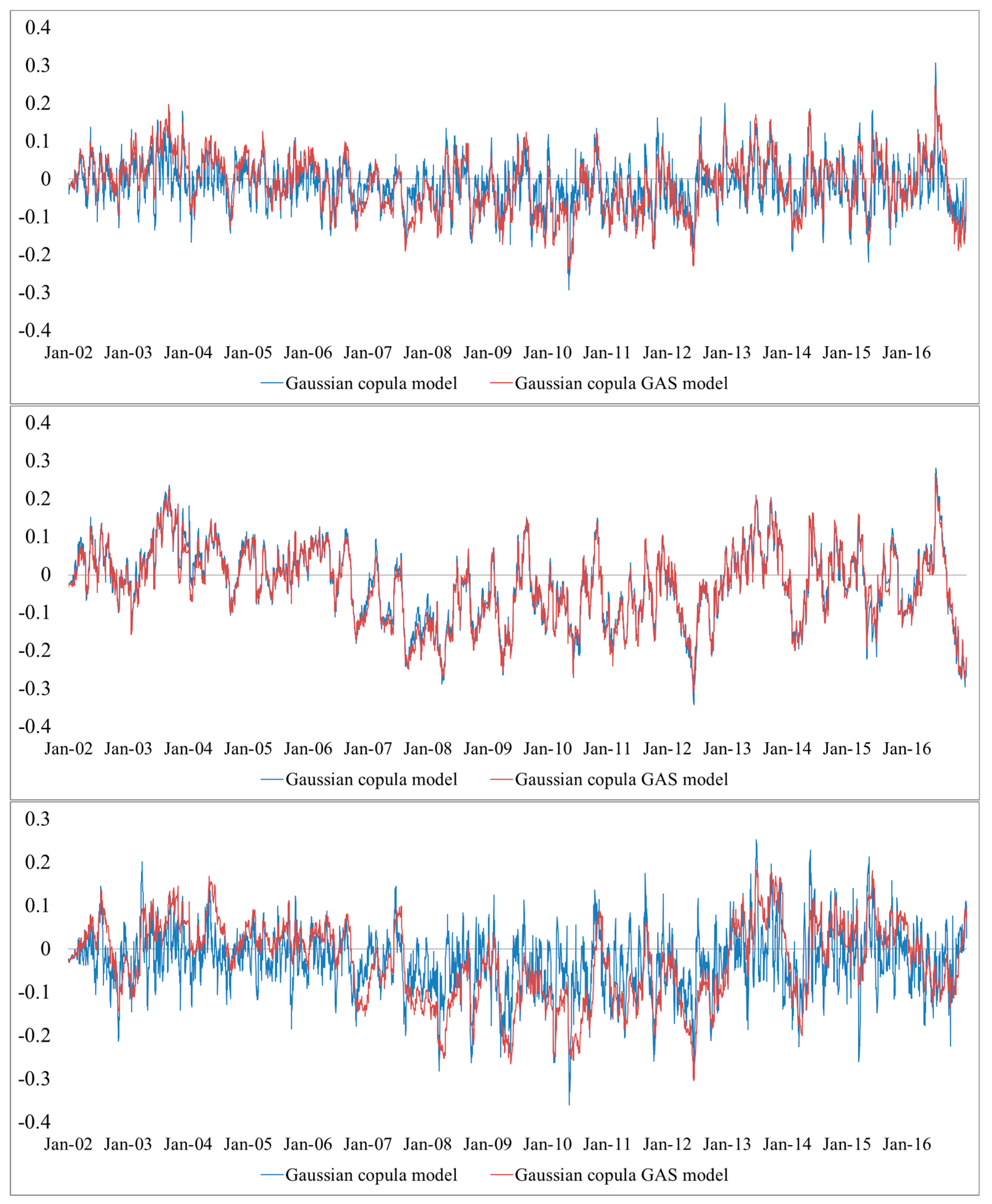
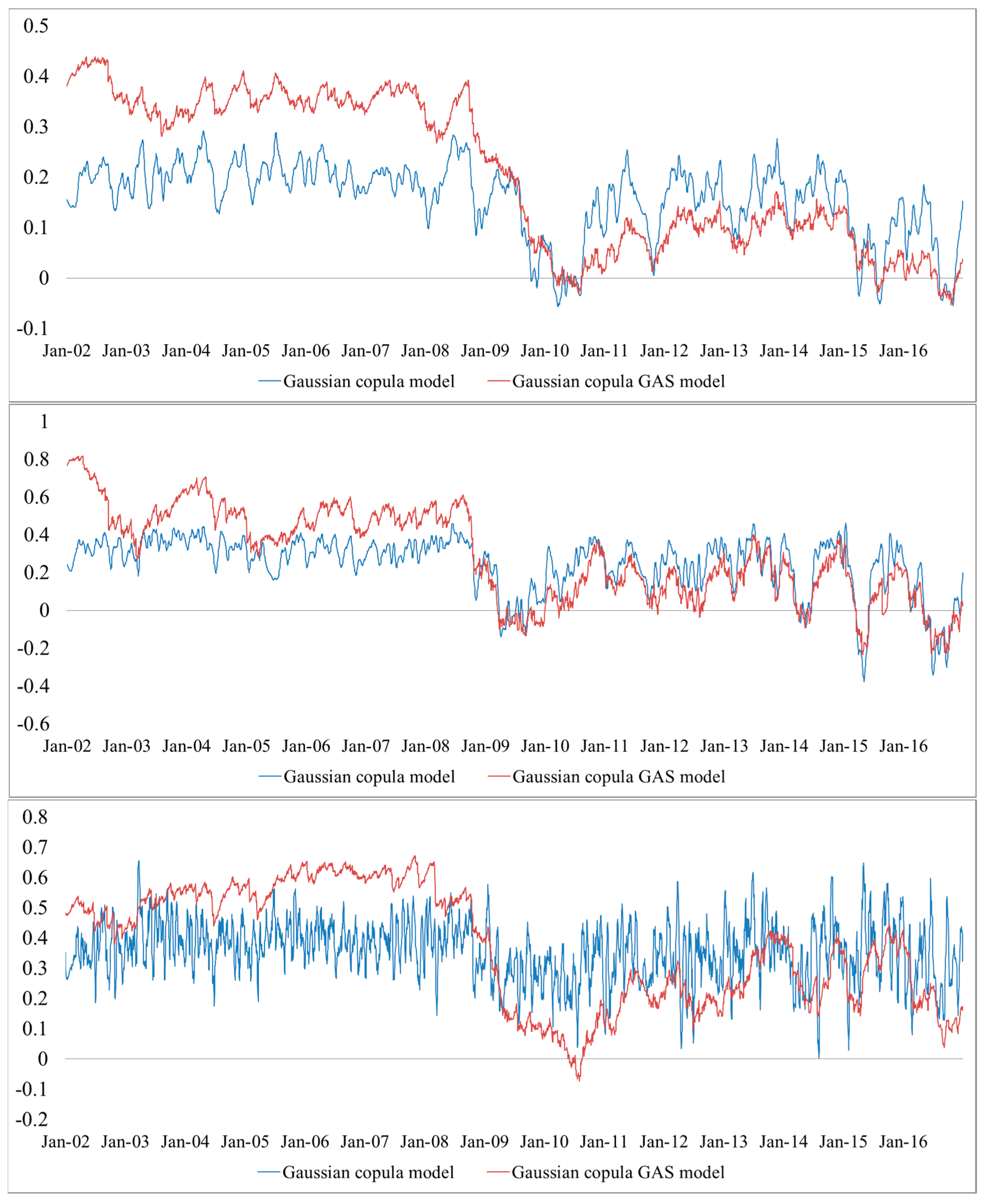
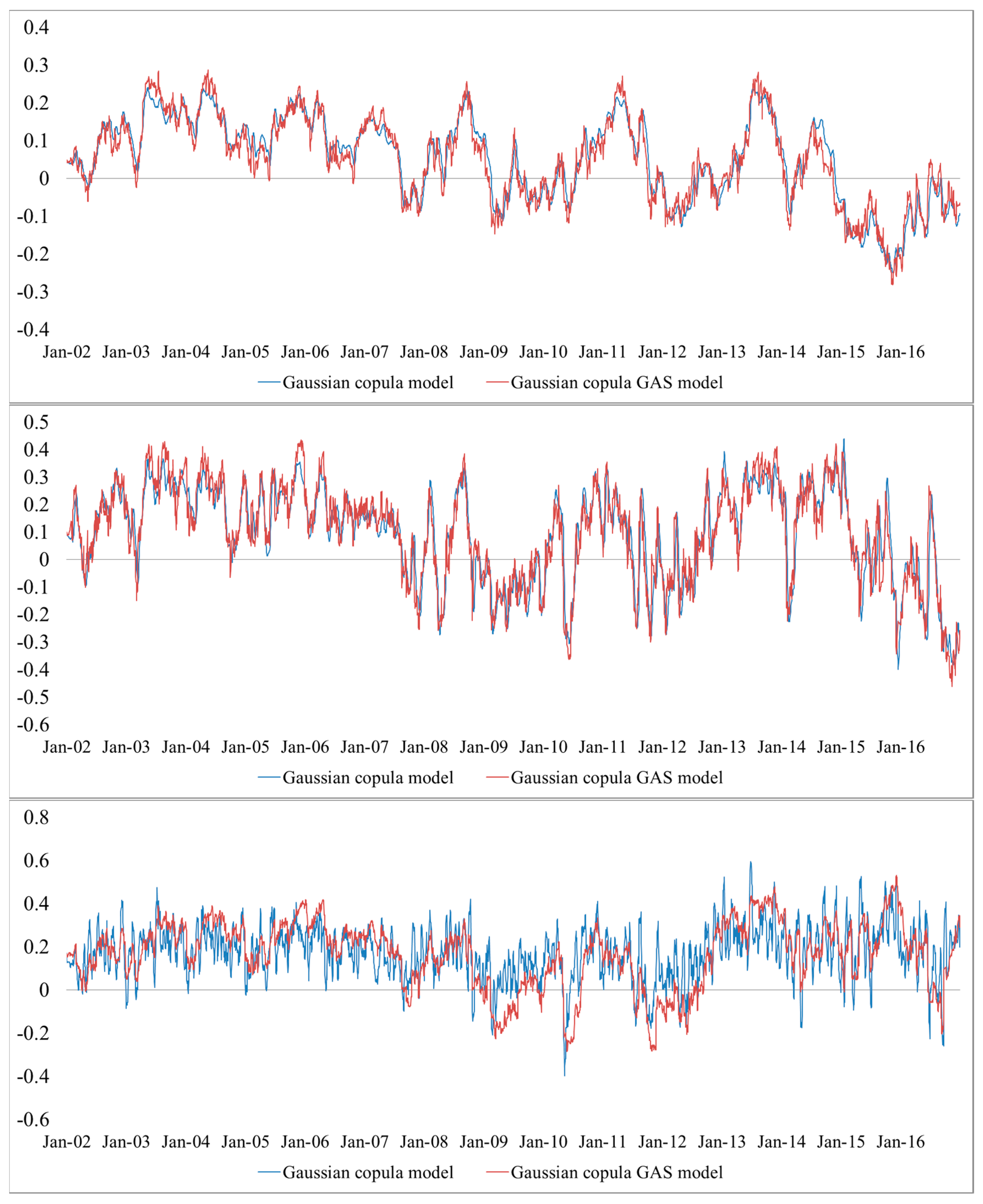
To illustrate the integration process between the CEEC-3 and Germany, Figure 1, Figure 2 and Figure 3 plot their estimated dynamic correlations from the Gaussian copula GAS model for the 3-year, 5-year, and 10-year yields. These figures illustrate the high (low) dependence of the government securities markets in the long term (short term). In addition, the Czech Republic showed the highest dependence with Germany, while Hungary showed the lowest. In particular, the structures of dynamic correlations for Hungary were different from that of Poland and the Czech Republic, which may due to the fact that Hungary has been experiencing a fiscal crisis since 2012.

Meanwhile, to see how EU accession, the global financial crisis, and the European debt crisis affected dependence, we employed the multiple breakpoint test to examine the influence of dependence based on global information citations (

Table 6. Breakpoint test based on global information citations.

	3-Year	5-Year	10-Year
Czech–Germany
Breakpoint 1	9/28/2004	12/24/2004	12/12/2003
Breakpoint 2	8/23/2007	10/17/2008	3/05/2007
Breakpoint 3	8/04/2009	9/29/2010	2/12/2009
Breakpoint 4	12/28/2011	10/22/2012	1/25/2011
Breakpoint 5			1/11/2013
Poland–Germany
Breakpoint 1	5/01/2006	4/01/2004	4/01/2004
Breakpoint 2	11/05/2008	5/15/2006	5/15/2006
Breakpoint 3	10/18/2010	10/22/2008	10/22/2008
Breakpoint 4	1/21/2013	10/04/2010	10/04/2010
Breakpoint 5		11/07/2012	11/07/2012
Hungary–Germany
Breakpoint 1	3/20/2007	9/25/2006	8/07/2007
Breakpoint 2	12/04/2009	6/05/2009	9/27/2010
Breakpoint 3	12/10/2012	12/07/2012	1/04/2013
Breakpoint 4
Breakpoint 5

Notes: The date is given by Month/Day/Year. We chose the numbers of the breakpoint date according to the SIC.

). In general, we found that these three events affected dependence significantly. As shown in Figure 1, Figure 2 and Figure 3, the correlation significantly increased before the examined CEEC-3 countries became EU members, in the global financial crisis period, and in the European debt crisis period. Combining the results presented in Table 6 confirmed that financial contagion occurred during these two crises. Meanwhile, the significant increase in correlation before EU accession may have been caused by the expectations of market participants and requirements of being EU members. After the global financial crisis, there was a significant decrease in dependence, perhaps because of capital regulations and market segmentation [14].

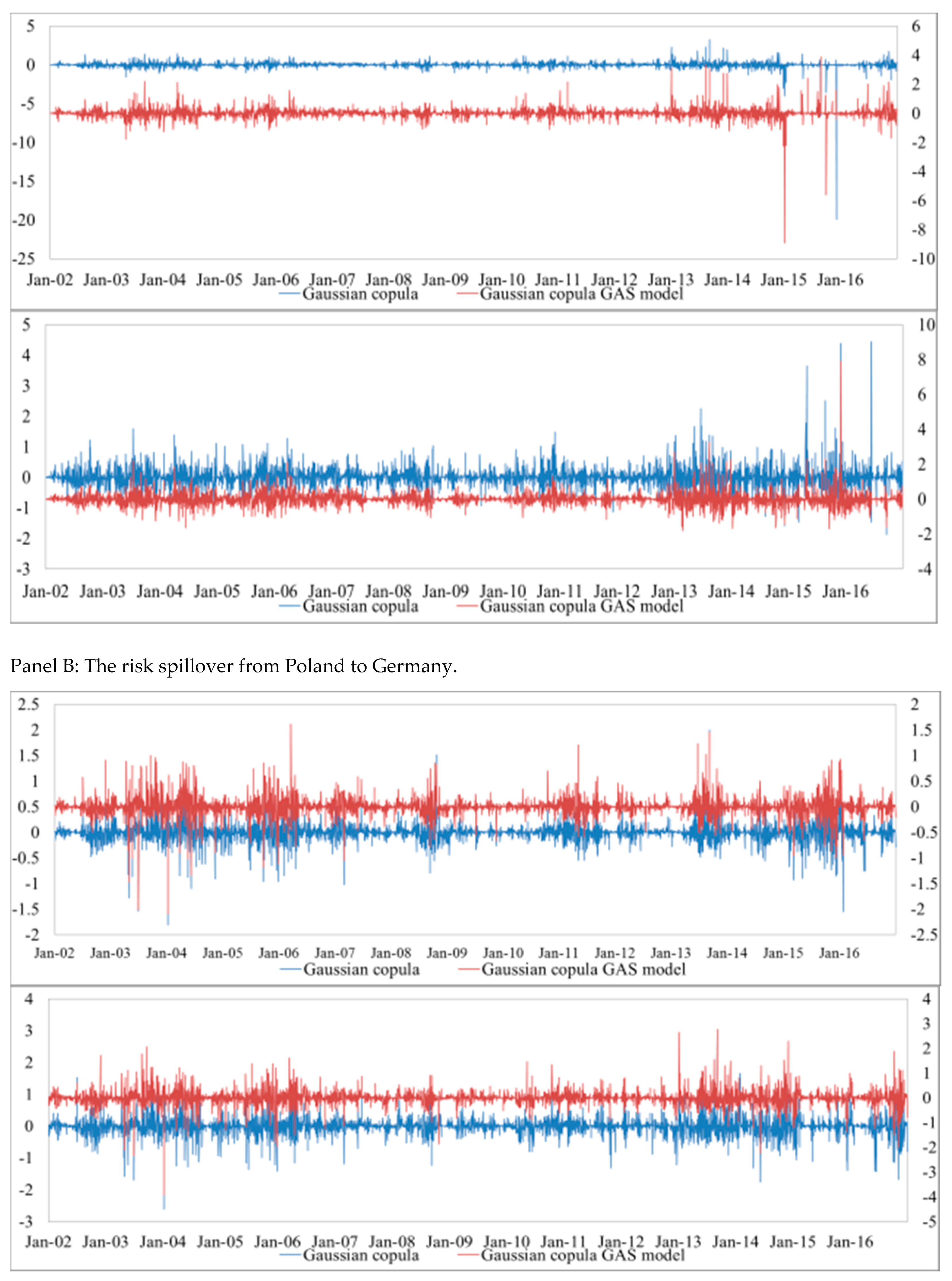
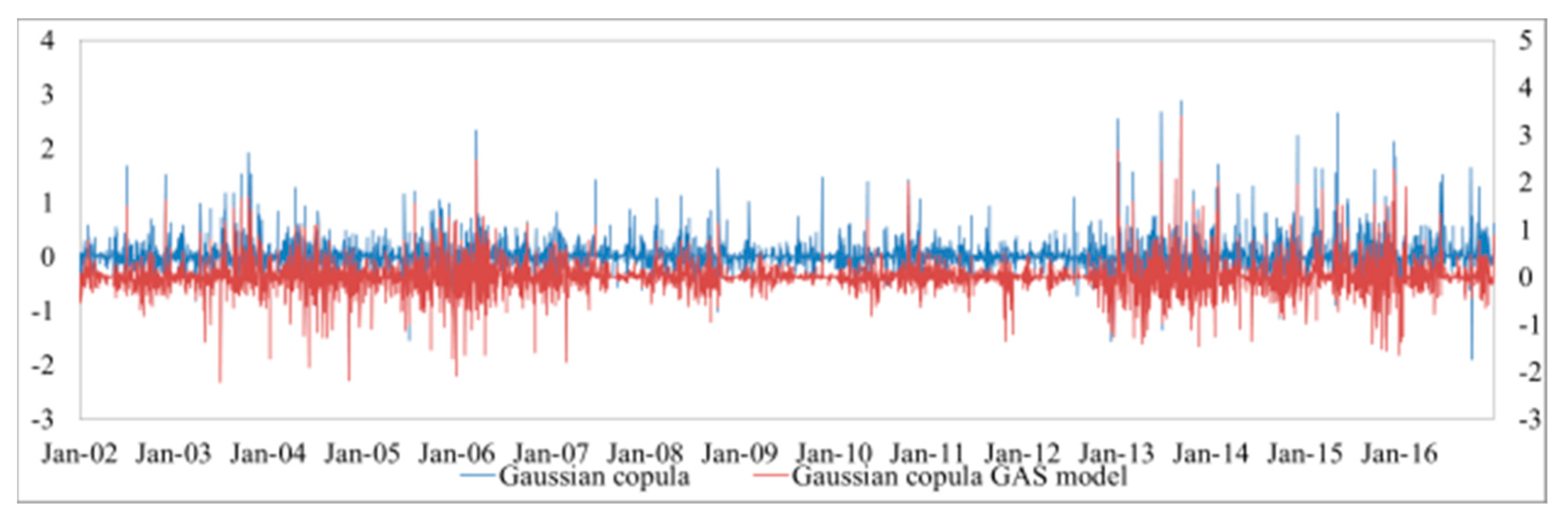
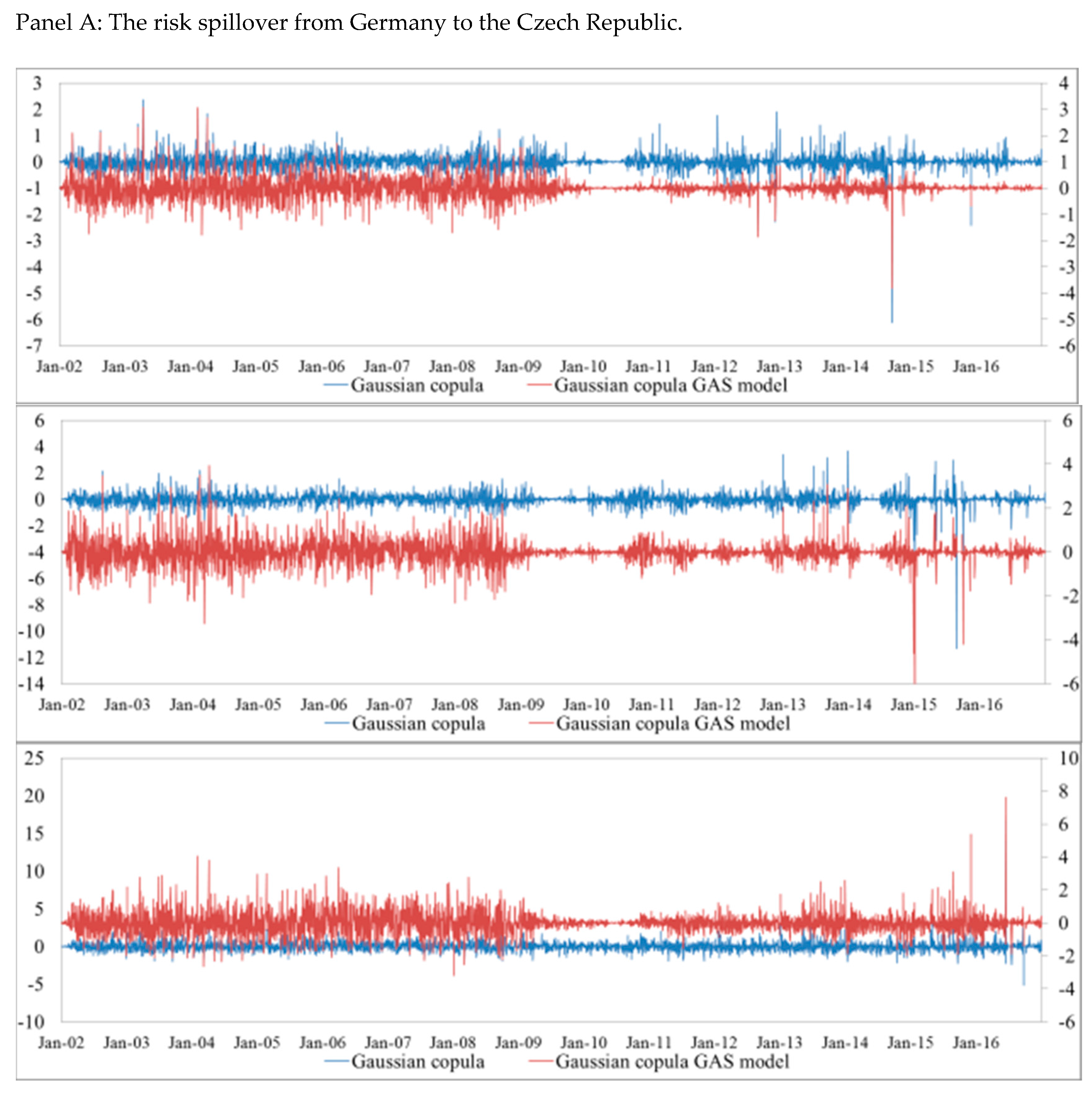
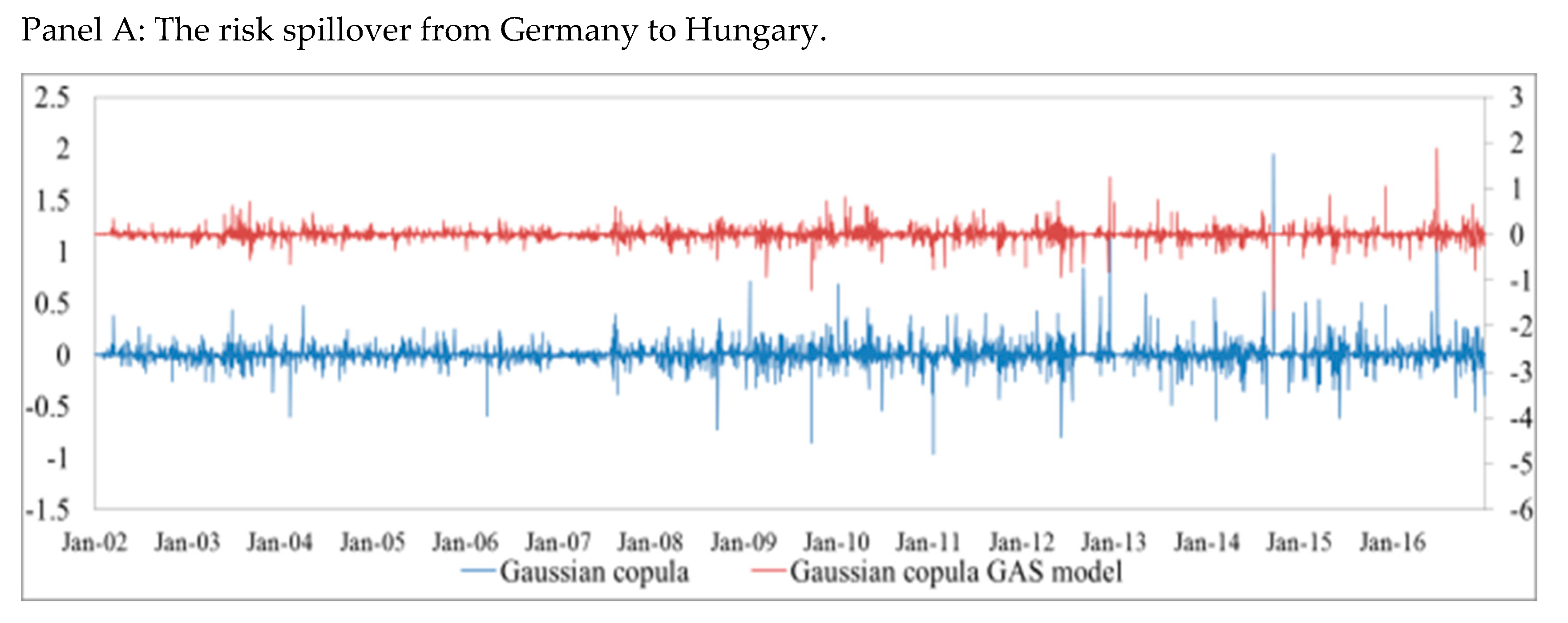
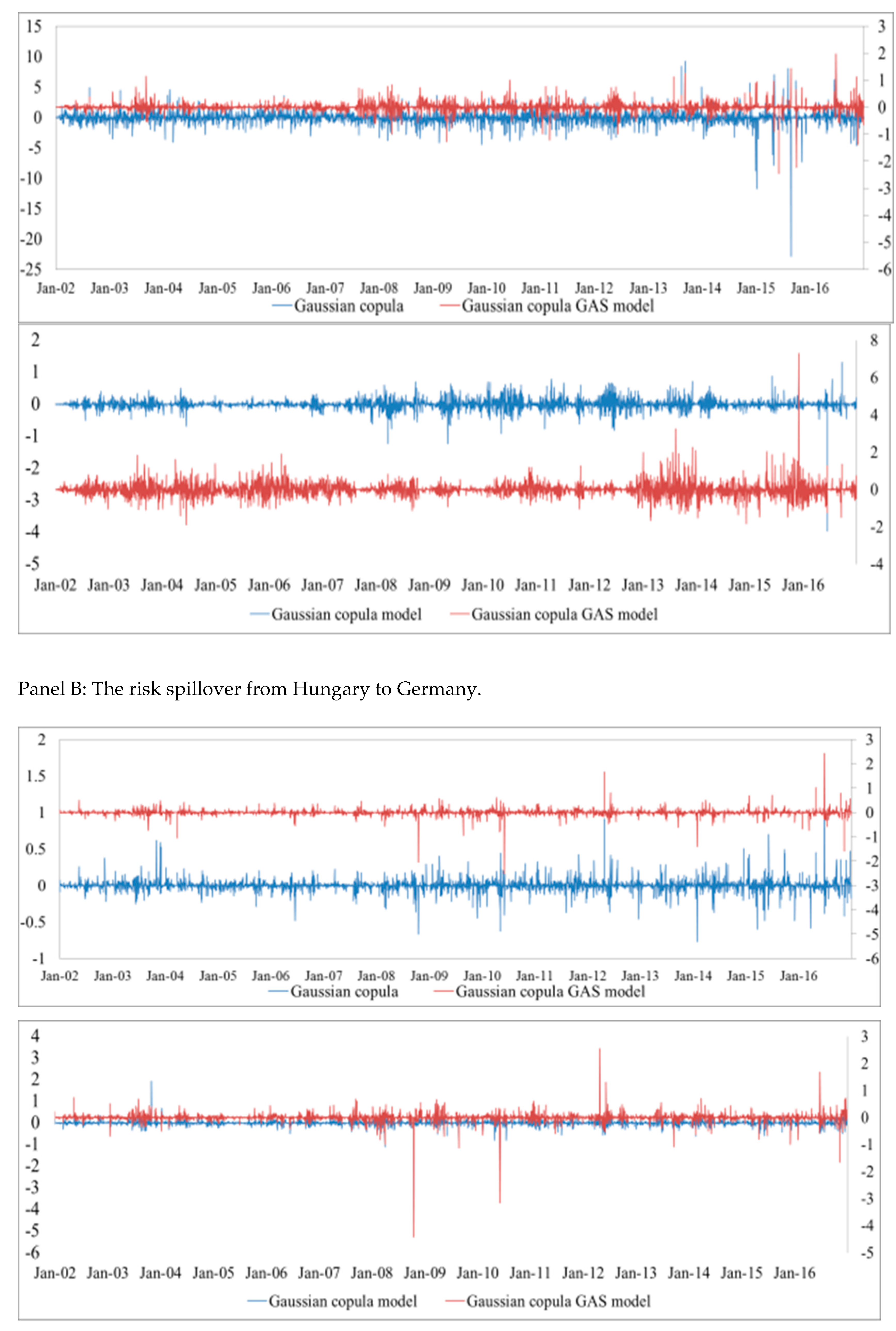
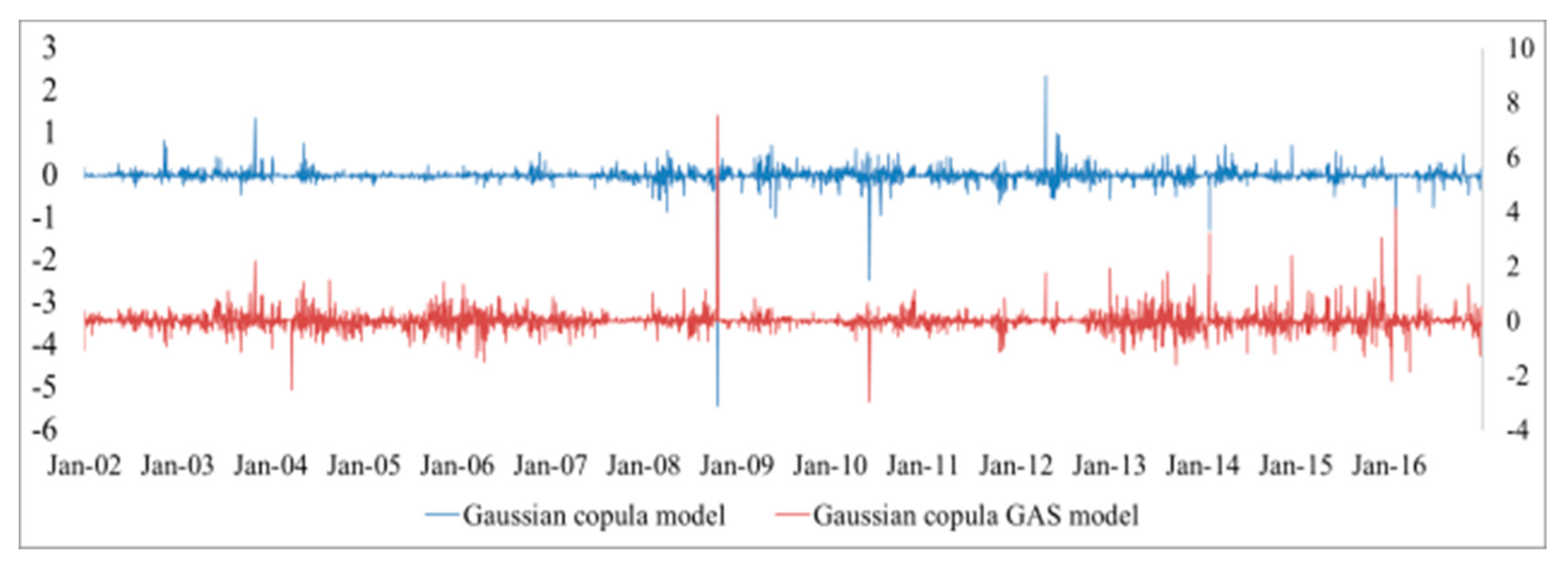
4.3. Risk Spillovers

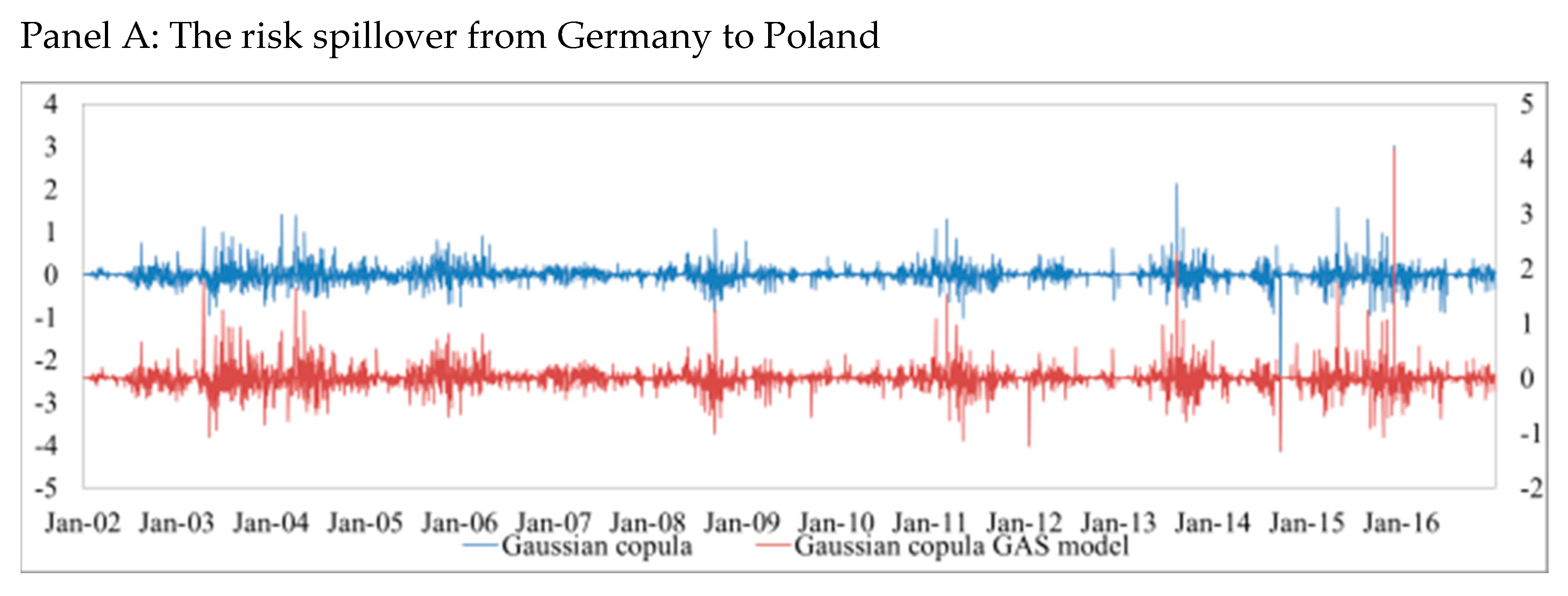
Figure 4, Figure 5 and Figure 6 plot the estimations of ΔCoVaR. Specifically, the blue line reflects the spillover effect from Germany to the CEEC-3 and the red line reflects the spillover effect from the CEEC-3 to Germany (The CoVaR estimations are available from the authors upon request). As shown in these figures, the GAS-based Gaussian copula model was more sensitive than the Gaussian copula model as expected. Moreover, the empirical evidence indicated that the German systemic risk was low and relatively stable, while the CEEC-3 systemic risk was high and variant. Specifically, Poland showed the lowest systemic risk, whereas Hungary showed the highest. Since the impact of the global financial crisis was reflected in the abrupt increase in the ΔCoVaR value, we observed that the European debt crisis increased the ΔCoVaR value for both the German systemic risk and the CEEC-3 systemic risk. Finally, the ΔCoVaR of long-term government securities fluctuated more widely than that for short-term government securities in these countries. These results suggest that the systemic risk is higher for both the CEEC-3 countries and for longer-term bonds.

Furthermore, our empirical evidence also showed that ΔCoVaR volatility increased substantially for the countries in crisis. The reason may be the uncertainty of the government securities markets and implementation of stabilization policies by the European Central Bank and International Monetary Fund. These actions also provoke sudden changes in investor expectations. All the evidence on the systemic risk dynamics was consistent with the idea that the crisis not only had spillover effects on countries with weak economic fundamentals (e.g., Hungary, which had the highest systemic risk), but also had contagion effects for both the CEEC-3 and Germany.

4.4. Dynamic SJC Copula

To ascertain how these events affected the dependence of the government securities markets in CEEC-3 and Germany, we employed the dynamic SJC (symmetrized Joe-Clayton) copula proposed by Patton [17] to investigate positive and negative events. In particular, we examined the dynamic tail correlations in these markets to find the possibility of contagion or fight to quality. Generally, correlations exist across the markets, but tail correlations do not. If the tail correlations exist across the markets, the contagion or fight to quality will more likely occur as the contagion is more likely to be related to the lower tail dependence, while the fight to quality is more likely to be connected to the upper dependence. Following Patton [17], the density of the SJC copula is

$$c_{SJC}\left(u,v|{\tau }^U,{\tau }^L\right)=0.5[c_{JC}\left(u,v|{\tau }^U,{\tau }^L\right)+c_{JC}\left(1-u,1-v|{\tau }^U,{\tau }^L\right)+u+v-1]$$

(14)

The SJC copula is symmetric when ${\tau }^U={\tau }^L$ and asymmetric otherwise. To estimate the time-varying dependence structure for the conditional copula, we assumed that the dependence parameter was determined by past information and that it followed an autoregressive moving average, or ARMA (1,10)-type process. Therefore, the dynamics of upper and lower tail dependence can be expressed as Equations (15) and (16), respectively:

$${\tau }_t^U={{\displaystyle \prod }}^{\text{}}({\beta }_U^{SJC}{\tau }_{t-1}^U+{\omega }_U^{SJC}+{\gamma }_U^{SJC}\frac{1}{10}{{\displaystyle \sum }}_{i=1}^{10}\left|u_{t-i}-{\upsilon }_{t-i}\right|)$$

(15)

$${\tau }_t^L={{\displaystyle \prod }}^{\text{}}({\beta }_L^{SJC}{\tau }_{t-1}^L+{\omega }_L^{SJC}+{\gamma }_L^{SJC}\frac{1}{10}{{\displaystyle \sum }}_{i=1}^{10}\left|u_{t-i}-{\upsilon }_{t-i}\right|)$$

(16)

where ${\displaystyle \prod }$ is the logistic transformation to keep ${\tau }^U$ and ${\tau }^L$ within the (0, 1) interval. We also estimated the parameters based on the MSML estimation method.

Table 6 reports the estimation results. For the copula function, $\beta$ denotes the degree of persistence and $\gamma$ represents the adjustment in the dependence process. As shown in

Table 7. Estimation results of the SJC copula model.

	3-Year	5-Year	10-Year
Czech–Germany
ωU	0.439 (0.302)	0.072 (0.078)	0.041 (0.015) ***
γU	−2.671 (0.431) ***	−0.368 (0.027) ***	−0.196 (0.072) ***
βU	0.914 (0.051) ***	0.988 (0.017) ***	0.991 (0.004) ***
ωL	0.044 (0.059)	0.094 (0.092)	0.079 (0.023) ***
γL	−0.203 (0.078) ***	−0.453 (0.466)	−0.399 (0.176) **
βL	0.995 (0.008) ***	0.986 (0.017) ***	0.988 (0.007) ***
Log-Likelihood	78.469	230.020	352.096
Poland–Germany
ωU	−1.035 (0.131) ***	−0.180 (0.696)	0.162 (0.065) ***
γU	−0.484 (0.465)	−0.538 (1.975)	−0.961 (0.358) ***
βU	2.106 (2.253)	1.256 (1.353)	0.963 (0.014) ***
ωL	−3.912 (3.450)	−4.751 (2.950)	−1.115 (1.018)
γL	−0.917 (1.507)	−0.658 (0.900)	−9.421 (1.431) ***
βL	0.903 (1.659)	0.356 (0.371)	−0.112 (0.237)
Log-Likelihood	2.261	22.933	83.667
Hungary–Germany
ωU	−4.377 (1.259) ***	−4.849 (3.180)	−4.556 (2.918)
γU	−1.021 (18.862)	−1.132 (26.387)	−1.079 (37.612)
βU	0.801 (1.039)	0.707 (0.415) *	0.795 (1.840)
ωL	−9.462 (1.007) ***	−9.534 (0.980) ***	−9.473 (1.071) ***
γL	−1.185 (2.827)	−1.406 (2.367)	−1.351 (5.567)
βL	0.303 (0.111) **	0.301 (0.106) ***	0.317 (0.154) **
Log-Likelihood	−11.042	−17.312	−17.291

Notes: *, **, and *** represent significance at the 10%, 5%, and 1% levels, respectively.

, the parameters $\gamma$ and $\beta$ are significant only for the Czech Republic and Germany for all maturities, and for Poland and Germany for the 10-year maturity, suggesting that significant variance and strong dependency existed over time in these pairs.

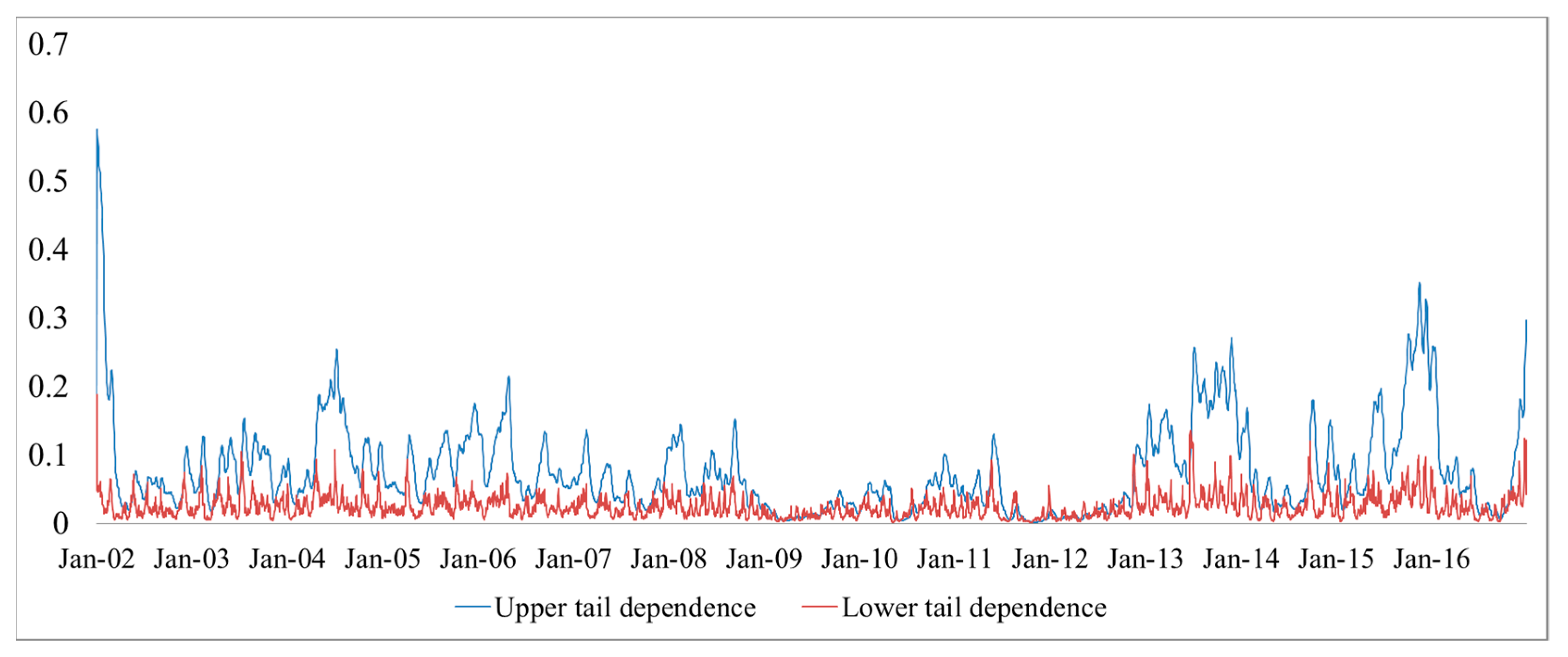
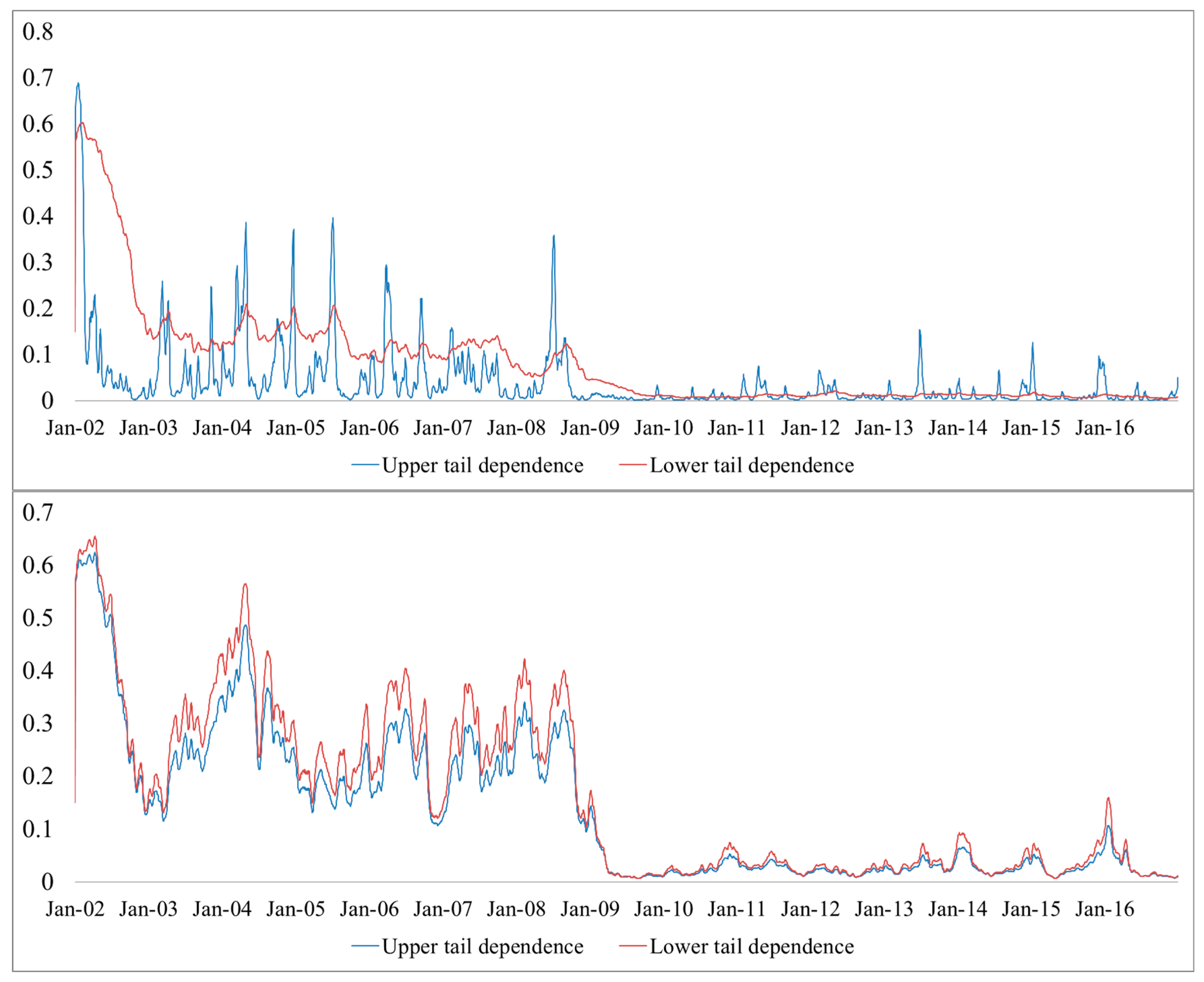
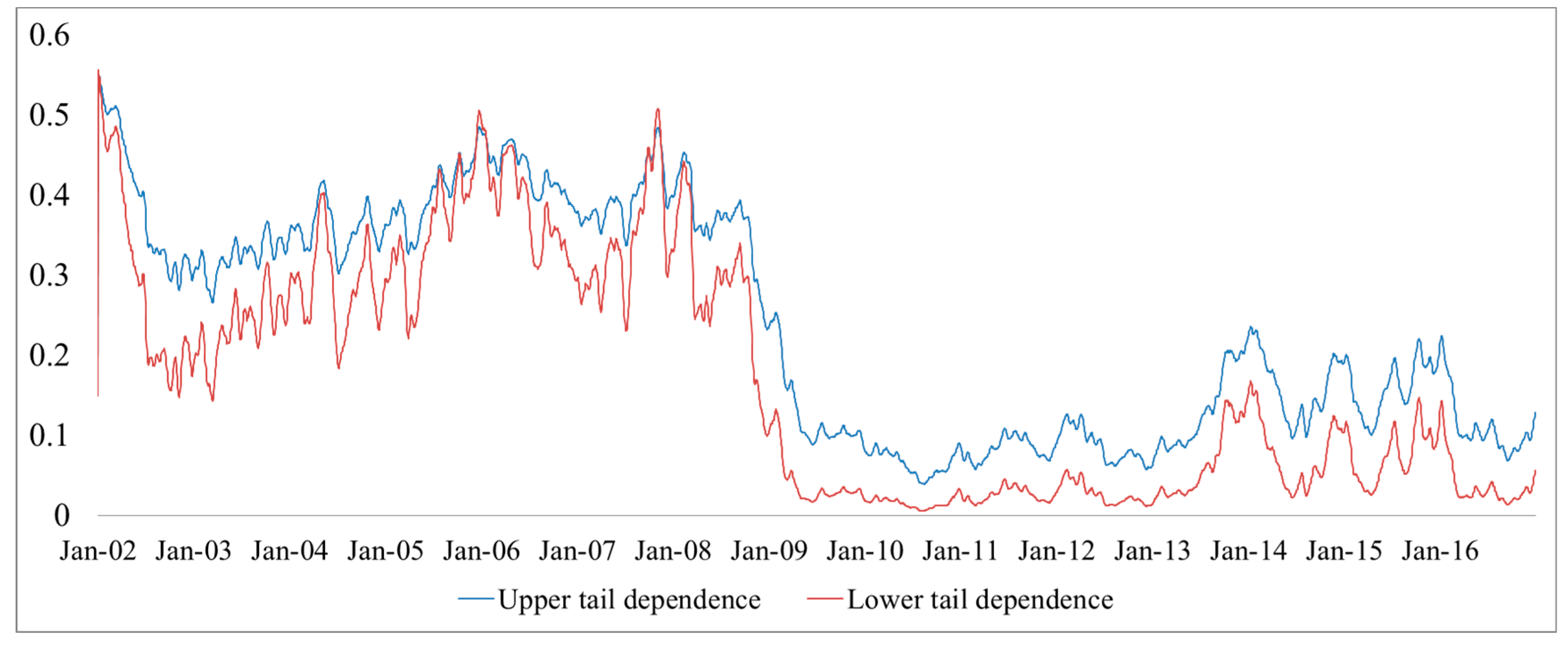
Figure 7 and Figure 8 compare the time paths of the conditional lower and upper tail dependence based on the SJC copula for Poland and the Czech Republic, respectively. In general, we found that the conditional upper tail dependence was greater and fluctuated more than the conditional lower tail dependence for Poland and for the 3- and 5-year government securities markets because the value of ${\omega }^L$ was less than that of ${\omega }^U$. Moreover, the variation degree increased as maturities increased. However, the conditional upper tail dependence fluctuated less than the conditional lower tail dependence for the Czech Republic in the 10-year government securities market. In addition, the dynamic process of tail dependence was not well specified for the Poland–Germany and Hungary–Germany pairs since the parameters $\gamma$ and $\beta$ were insignificant. Thus, they were omitted.

Meanwhile, these results also indicated that the Czech Republic showed the highest dependence with Germany. In addition, both positive and negative news from Germany significantly affected dependence, with the former having a larger influence than the latter, which was consistent with the findings of Yang and Hamori [7]. In contrast to Büttner and Hayo [4] as well as Yang and Hamori [7,8], however, we provided the dynamic process of dependence between the CEEC-3 and Germany and showed that the positive and negative news affected dependence dynamically. Figure 7 and Figure 8 also confirmed that financial contagion occurred during the global financial and European debt crises, consistent with the evidence provided by Boubakri and Guillaumin [14].

5. Conclusions

In this study, we investigated the dependence of the government securities markets in the CEEC-3 and Germany across maturities by employing the GAS-based dynamic Gaussian copula model. We found a high dependence of these government securities markets in the long maturity, but low dependence in the short maturity. In addition, the Czech Republic showed the highest dependence with Germany, while Hungary showed the lowest. Consistent with the findings of Pozzi and Wolswijk [9], by employing the breakpoint test, we also confirmed that EU accession, the global financial crisis, and the European debt crisis caused structural changes in the dynamic correlation.

Furthermore, by employing the ΔCoVaR risk measure, we observed that the German systemic risk was low and relatively stable, while the CEEC-3 systemic risk was high and variant. By considering different time horizons, we showed that the long-run bond ΔCoVaR was higher than the short-run bond ΔCoVaR. This evidence on the systemic risk dynamics shows that the crisis not only had spillover effects on countries with weak economic fundamentals (e.g., Hungary, which has the highest systemic risk), but also had contagion effects for both the CEEC-3 and Germany.

We also employed the SJC copula to examine the dynamic tail dependence among these countries. By comparing and contrasting the results from the dynamic Gaussian copula, we found that both positive and negative news from Germany significantly affected dependence with the Czech Republic, with the former having a larger influence than the latter. These results also showed that the dependence structure between the CEEC-3 and Germany was asymmetric. In addition, we confirmed that the Czech Republic showed the highest dependence with Germany and that financial contagion occurred during the global financial crisis and European debt crisis.

Our results have at least one implication for policymakers and two implications for investors. For policymakers, although the integration of the financial markets in the CEEC-3 has decreased since 2008 owing to market segmentation, becoming an EU member has increased the degree of dependence with European financial markets. For investors, diversification benefits still exist, especially since the global financial crisis. In addition, the dynamic correlations for these countries are more sensitive to positive shocks, indicating that government securities markets remain a good investment, even during a crisis period. Additionally, the risk spillovers from the German government securities market may not be a large concern when compared with those from the CEEC-3 countries.

References

- Engle, R. Autoregressive conditional heteroskedasticity with estimates of the variance of United Kingdom inflation. Econometrica 1982, 50, 987–1007. [Google Scholar] [CrossRef]
- Bollerslev, T. A conditionally heteroskedastic time series model for speculative prices and rates or return. Rev. Econ. Stat. 1987, 69, 542–547. [Google Scholar] [CrossRef]
- Engle, R. Dynamic conditional correlation: A simple class of multivariate generalized autoregressive conditional heteroskedasticity models. J. Bus. Econ. Stat. 2002, 20, 339–350. [Google Scholar] [CrossRef]
- Büttner, D.; Hayo, B. News and correlations of CEEC-3 financial markets. Econ. Model. 2010, 27, 915–922. [Google Scholar] [CrossRef]
- Yang, L.; Hamori, S. EU accession, contagion effects, and financial integration: Evidence from CEEC-3 bond markets. Transit. Stud. Rev. 2013, 20, 179–189. [Google Scholar] [CrossRef]
- Kumar, M.S.; Okimoto, T. Dynamics of international integration of government securities’ markets. J. Bank. Financ. 2011, 35, 142–154. [Google Scholar] [CrossRef]
- Yang, L.; Hamori, S. Dependence structure between CEEC-3 and German government securities markets. J. Int. Financ. Mark. Inst. Money 2014, 2, 109–125. [Google Scholar] [CrossRef]
- Yang, L.; Hamori, S. Interdependence between the bond markets of CEEC-3 and Germany: A wavelet coherence analysis. N. Am. J. Econ. Financ. 2015, 32, 124–138. [Google Scholar] [CrossRef]
- Pozzi, L.; Wolswijk, G. The time-varying integration of euro area government bond markets. Eur. Econ. Rev. 2012, 56, 36–53. [Google Scholar] [CrossRef]
- Bekiros, S. Forecasting with a state space time-varying parameter VAR model: Evidence from the Euro area. Econ. Model. 2014, 38, 619–626. [Google Scholar] [CrossRef]
- Creal, D.D.; Koopman, S.J.; Lucas, A. Generalized autoregressive score models with applications. J. Appl. Econ. 2013, 28, 777–795. [Google Scholar] [CrossRef]
- Oh, D.H.; Patton, A.J. Modelling dependence in high dimensions with factor copulas. J. Bus. Econ. Stat. 2017, 35, 139–154. [Google Scholar] [CrossRef]
- Creal, D.D.; Tsay, R.S. High dimensional dynamic stochastic copula models. J. Econ. 2015, 189, 335–345. [Google Scholar] [CrossRef]
- Boubakri, B.; Guillaumin, C. Financial integration and currency risk premium in CEECs: Evidence from the ICAPM. Emerg. Mark. Rev. 2011, 12, 460–484. [Google Scholar] [CrossRef]
- Tobias, A.; Brunnermeier, M.K. CoVaR. Am. Econ. Rev. 2016, 106, 1705–1741. [Google Scholar]
- Girardi, G.; Ergün, A.T. Systemic risk measurement: Multivariate GARCH estimation of CoVaR. J. Bank. Financ. 2013, 37, 3169–3180. [Google Scholar] [CrossRef]
- Patton, A.J. Modelling asymmetric exchange rate dependence. Int. Econ. Rev. 2006, 47, 527–556. [Google Scholar] [CrossRef]
- Glosten, L.R.; Jagannathan, R.; Runkle, D. On the relation between the expected value and the volatility of the nominal excess return on stocks. J. Financ. 1993, 48, 1779–1801. [Google Scholar] [CrossRef]
- Engle, R.; Ng, V.K. Measuring and testing the impact of news on volatility. J. Financ. 1993, 48, 1749–1778. [Google Scholar] [CrossRef]
- Nelson, D.B. Conditional heteroskedasticity in asset returns: A new approach. Econometrica 1991, 59, 347–370. [Google Scholar] [CrossRef]
- Hansen, B.E. Autoregressive conditional density estimation. Int. Econ. Rev. 1994, 35, 705–730. [Google Scholar] [CrossRef]
- Akaike, H. Information theory and an extension of the maximum likelihood principle. In 2nd International Symposium on Information Theory; Petrov, B., Csaki, F., Eds.; Akademia Kadio: Budapest, Hungary, 1973; pp. 267–281. [Google Scholar]
- Hafner, C.M.; Manner, H. Dynamic stochastic copula models: Estimation, inference and applications. J. Appl. Econ. 2012, 27, 269–295. [Google Scholar] [CrossRef]
- Manner, H.; Segers, J. Tails of correlation mixtures of elliptical copulas. Insur. Math. Econ. 2011, 48, 153–160. [Google Scholar] [CrossRef]
- Avdulaj, K.; Barunik, J. Are benefits from oil–stocks diversification gone? New evidence from a dynamic copula and high frequency data. Energy Econ. 2015, 51, 31–44. [Google Scholar] [CrossRef]
- Reboredo, J.C.; Ugolini, A. Systemic risk in European sovereign debt markets: A CoVaR-copula approach. J. Int. Money Financ. 2015, 51, 214–244. [Google Scholar] [CrossRef]
- McAleer, M. Stationarity and invertibility of a dynamic correlation matrix. Kybernetika 2018. forthcoming. [Google Scholar] [CrossRef]
- Schwarz, G. Estimating the Dimension of a Model. Ann. Stat. 1978, 6, 461–464. [Google Scholar] [CrossRef]
Figure 1.
Dynamic correlations between Hungary and Germany. Notes: This figure plots the estimated dynamic correlations between Hungary and Germany from the Gaussian copula and Gaussian copula GAS models for 3-year yields (top), 5-year yields (middle), and 10-year yields (bottom).
Figure 2.
Dynamic correlations between Czech Republic and Germany. Notes: This figure plots the estimated dynamic correlations between Czech Republic and Germany from the Gaussian copula and Gaussian copula GAS models for 3-year yields (top), 5-year yields (middle), and 10-year yields (bottom).
Figure 3.
Dynamic correlations between Poland and Germany. Notes: This figure plots the estimated dynamic correlations between Poland and Germany from the Gaussian copula and Gaussian copula GAS models for 3-year yields (top), 5-year yields (middle), and 10-year yields (bottom).
Figure 4.
ΔCoVaR between Poland and Germany. Notes: This figure plots the estimated ΔCoVaR between Poland and Germany from the Gaussian copula and Gaussian copula GAS models for 3-year yields (top), 5-year yields (middle), and 10-year yields (bottom) in the panel (A,B).
Figure 5.
ΔCoVaR between the Czech Republic and Germany. Note: This figure plots the estimated ΔCoVaR between the Czech Republic and Germany from the Gaussian copula and Gaussian copula GAS models for 3-year yields (top), 5-year yields (middle), and 10-year yields (bottom) in the panel (A,B).
Figure 6.
ΔCoVaR between Hungary and Germany. Note: This figure plots the estimated ΔCoVaR between Hungary and Germany from the Gaussian copula and Gaussian copula GAS models for 3-year yields (top), 5-year yields (middle), and 10-year yields (bottom) in the panel (A,B).
Figure 7.
Dynamic tail correlations between Poland and Germany. Note: This figure plots the estimated dynamic tail correlations between Poland and Germany from the SJC copula model for 10-year yields.
Figure 8.
Dynamic tail correlations between the Czech Republic and Germany. Note: This figure plots the estimated dynamic tail correlations between the Czech Republic and Germany from the SJC copula model for 3-year yields (top), 5-year yields (middle), and 10-year yields (bottom).