Article

Congenital Gastrointestinal Anomalies in Europe 2010–2019: A Geo-Spatiotemporal and Causal Inferential Study of Epidemiological Patterns in Relationship to Cannabis- and Substance Exposure

by
Albert Stuart Reece
1,2,* and
Gary Kenneth Hulse
1,2
1
Division of Psychiatry, University of Western Australia, Crawley, WA 6009, Australia
2
School of Medical and Health Sciences, Edith Cowan University, Joondalup, WA 6027, Australia
*
Author to whom correspondence should be addressed.
Gastroenterol. Insights 2023, 14(1), 64-109; https://doi.org/10.3390/gastroent14010007
Submission received: 3 January 2023 / Revised: 31 January 2023 / Accepted: 9 February 2023 / Published: 23 February 2023
(This article belongs to the Collection Advances in Gastrointestinal Cancer)

Abstract

:
Introduction: Congenital anomalies (CA’s) of most of the gastrointestinal tract have been linked causally with prenatal or community cannabis exposure. Therefore, we studied this relationship in Europe. Methods: CA data were from Eurocat. Drug-use data were sourced from the European Monitoring Centre for Drugs and Drug Addiction. Income data were taken from the World Bank. Results: When countries with increasing rates of daily cannabis use were compared with those which were not, the overall rate of gastrointestinal CA’s (GCA’s) was higher in the former group (p = 0.0032). The five anomalies which were related to the metrics of cannabis exposure on bivariate analysis were bile duct atresia, Hirschsprungs, digestive disorders, annular pancreas and anorectal stenosis or atresia. The following sequence of GCA’s was significantly linked with cannabis metrics at inverse-probability-weighted-panel modelling, as indicated: esophageal stenosis or atresia, bile duct atresia, small intestinal stenosis or atresia, anorectal stenosis or atresia, Hirschsprungs disease: p = 1.83 × 10⁻⁵, 0.0046, 3.55 × 10⁻¹², 7.35 × 10⁻⁶ and 2.00 × 10⁻¹², respectively. When this GCA series was considered in geospatial modelling, the GCA’s were significantly cannabis-related from p = 0.0003, N.S., 0.0086, 6.652 × 10⁻⁵, 0.0002, 71.4% of 35 E-value estimates and 54.3% minimum E-values (mEVv’s) > 9 (high zone) and 100% and 97.1% > 1.25 (causality threshold). The order of cannabis sensitivity by median mEVv was Hirschsprungs > esophageal atresia > small intestinal atresia > anorectal atresia > bile duct atresia. Conclusions: Seven of eight GCA’s were related to cannabis exposure and fulfilled the quantitative criteria for epidemiologically causal relationships. Penetration of cannabinoids into the community should be carefully scrutinized and controlled to protect against exponential and multigenerational genotoxicity ensuing from multiple cannabinoids.

1. Introduction

Collectively, the gastrointestinal tract makes up one of the largest organs in the body and over 30% of body weight [1]. It is, therefore, of concern that anomalies of the gastrointestinal tract have been identified in association with prenatal or community cannabis exposure in several studies, including in reports from the Centres for Disease Control (CDC) Atlanta, Georgia with esophageal atresia with or without tracheoesophageal fistula [2], from Hawaii where pyloric stenosis and anal, rectal, large bowel atresia/stenosis were identified [3], from Australia where small bowel atresia and stenosis and anal stenosis were identified [4], and from the USA where esophageal atresia with or without tracheoesophageal fistula, rectal, large bowel atresia/stenosis, Hirschsprung disease and biliary atresia were identified [5]. Similarly, a relationship between cannabidiol and small bowel atresia and stenosis were positively identified in the USA [5]. Naturally, these reports considered collectively raise great concern as they identify most of the major organs along the length of the gastrointestinal tract (GIT), namely, esophagus, small and large intestines, anorectum and bile duct. We were naturally keen to study these issues further in the rich European datasets, particularly given that new data on European exposure to cannabinoids have recently been made available [6].
It is important to appreciate that research over several decades has identified multiple mechanisms by which cannabis exerts its genotoxic effects including grossly abnormal sperm morphology [7], high rates of abnormal oocyte division and oocyte loss [8], single- and double-stranded DNA breaks [9], chromosomal breaks [10,11], end-to-end chromosomal fusions and translocations [7,12], ring and chain chromosomal formation [7], double minute chromosomes [7,13], micronucleus formation [13,14], oxidation of DNA bases [9], epigenetic changes including reduced histone synthesis and post-translational acetylation and phosphorylation [15,16,17,18] and altered patterns of DNA methylation with both hyper-methylation and hypomethylation being reported [19,20,21,22,23,24,25,26,27]. Importantly, both the changes to the DNA methylome and those to the histones have been shown to be heritable via sperm and to affect the behaviour and immune response of offspring in rats [18,25,26,27]. The altered mental development of children prenatally exposed to cannabis has also been reported in all four of the long-term studies to have examined this association [28,29,30,31,32,33,34], and close relationships with autistic-like intellectual disabilities have also been reported [27,35,36,37,38,39].
It is important to bear in mind in discussing pathways towards and the phenomenology of cannabinoid teratogenesis that this forms a part of the overall picture of cannabis-related genotoxicity, which also includes cannabinoid-induced carcinogenesis [40,41,42,43,44,45,46,47,48,49] and cannabinoid-accelerated cellular and organismal ageing, which has also been demonstrated clinically [50,51]. It is important that this broader literature is also considered in the present context.
One of the key substrates of epigenomic reactions is the metabolic state of the cell and its mitochondrial metabolism. This is because mitochondria not only supply energy and substrates to the nucleus for genomic and epigenomic reactions, but they are also in close communication with the nucleus via mitonuclear and mitohormetic balance and can induce powerful cellular stress reactions when perturbed; thus, the disruption of mitochondrial metabolism necessarily modifies epigenomic stability. Many papers demonstrate that the dose–response relationship of cannabinoids with both genomic mutagenicity and mitochondrial toxicity is strongly exponential [52,53,54,55,56]. Moreover, this exponentiation of the dose–response effect has been extended to epidemiological studies where it has been repeatedly demonstrated that the passage from the fourth to fifth quintile of cannabinoid exposure is accompanied by a discontinuous quantum jump in congenital anomaly rates [5,57,58,59,60].
This is presumably also well demonstrated by the recent French experience—parts of France where large crops of cannabis are grown have suddenly reported 60-fold increases in the rates of calves and human babies being born without limbs [61,62,63], whilst this has not been reported in Switzerland, which is nearby where cannabis is not permitted to become involved in the food chain. Similar features presumably occur in cannabis-growing parts of the USA where atrial septal defects in states such as Kentucky and Mississippi have suddenly leaped to rates 20 time those of five years ago [64].
Of concern is the concomitant increase in prevalence rates of cannabis use, increased intensity of use on all or nearly all days, and increasing potency of Δ9-tetrahydrocannabinol (THC) in cannabis preparations—all of which imply a greatly increased community cannabinoid exposure [6,65] in a manner which launches society relatively abruptly into a higher cannabinoid dose-exposure range, where genotoxic effects will be more common. Given the multiple earlier reports noted above, the present study investigated continental European trends for digestive system disorders in the context of the changing continental cannabinoid environment in a formal, causal, inferential analytical paradigm and in its native space-time context.

2. Methods

Data: The data, which were analysed in this study on congenital anomalies, were obtained by direct download from the European Network of Population-Based Registries for Epidemiological Surveillance of Congenital Anomalies (EUROCAT) website [66]. The data variable which was the centre of our analytical attention was the total congenital anomaly rate, which is defined as being the sum total of the total live birth rate, the total miscarriage rate after 20 weeks of gestation and the total number of early termination for anomaly (ETOPFA) which was practised. Thus, this total congenital anomaly rate very usefully captured all forms of live births and major birthing complications.
Nations were chosen based upon the availability of their congenital anomaly data across the period from 2010 to 2019. Data on tobacco and alcohol consumption were sourced from online databases at the World Health Organization [67]. The unit of tobacco measured was the percentage of daily tobacco usage. The unit of alcohol measured was the amount in litres of pure alcohol consumed per capita per year. Drug-use data were taken from the European Monitoring Centre for Drugs and Drug Addiction (EMCDDA) [68]. The drugs of interest were amphetamines, cocaine and cannabis. The unit measured for amphetamine and cocaine was the prevalence of use in the last year. The major index of cannabis studied was the prevalence of use in the past month (prior to the completion of the data survey in each country). These data were supplemented by recent published descriptions of the mean THC concentration of the cannabis herb and resin available in each country [6,68], which are covariates described, respectively, as Herb_THC and Resin_THC, in the present report. Data on the prevalence of daily cannabis use were also taken from these sources—the data were also available on the EMCDDA website. Data on the median household income (measured in USD) were taken from the World Bank online sources [69].
Countries were divided in to two groups based on their cannabis status, as described in recent leading epidemiological reports of cannabis use in Europe [6]. Nations were either assigned to those with high and/or rising levels of daily cannabis use or low and/or falling rates of daily cannabis use based on the levels and use; the trends and results are reported in Supplementary Figure S4 in reference [6]. In this manner, Croatia, Germany, Italy, Belgium, the Netherlands, Norway, Portugal, France and Spain were categorized as nations which were undergoing increasing daily use, and Hungary, Bulgaria, Finland, Poland and Sweden were countries which were categorized as experiencing low or falling levels of daily cannabis use.
Derived Data: Because multiple measurements could be used to measure cannabis use and THC exposure, this created some ambiguities for analysis. These indices could evidently be combined in different ways. Hence, the past month cannabis use was multiplied by the THC concentration of cannabis herb and resin to derive a product for each. This metric was then multiplied by the interpolated daily-cannabis-use rate for both herb and resin products to derive further compound indices.
Data Imputation: Missing data were addressed by the use of linear interpolation. This technique was mainly applied to the data on rates of daily cannabis use. The EMCDDA dataset had only 59 datapoints in this dataset for this covariate for all these nations across this period. The dataset was partially completed by linear interpolation and an extra 70 datapoints were added, totalling 129 datapoints in all. Further details are provided in the Section 3. We were not able to identify any Swedish data for the THC concentration in cannabis resin in any of the years studied. However, it was noticed that the ratio of the THC concentration of cannabis resin to cannabis herb was quite steady in nearby Norway, with a value of 17.7, thus, this ratio was used together with the Swedish data for cannabis herb THC concentration to calculate an estimate of Swedish resin THC concentration. In a similar regard, Polish data for the THC concentration of cannabis resin were also unavailable. The ratio of the THC concentration of cannabis resin to cannabis herb in nearby Germany was available. This was used with the Polish herb THC concentration data to calculate and estimate the concentration of THC in cannabis resin.
Currently, extant geospatial techniques do not permit missing data. For this reason, absent data for Croatia for 2018 and 2019 were completed by the last observation carried forwards method. Absent data for the Netherlands were completed by the last observation carried backwards method. It was not possible to use the techniques of multiple imputation on this data as panel and geospatial methods have not been developed which accept imputed datasets neither at the time of conducting this analysis nor at the time of writing.
Statistics. R Studio version 1.4.1717 based on R version 4.1.1 from the Comprehensive R Archive Network and the R Foundation for Statistical Computing was used for data processing [70]. The statistical analysis of this data was conducted in December 2021. Data input and wrangling was performed using dplyr from the tidyverse [71]. Data were log-transformed as needed in the interests of approximating the normal distribution, as indicated by the results of the Shapiro–Wilks test. This test was performed in the R Base module. Graphs were drawn using ggplot2 also from the tidyverse [71]. ggplot2 was used together with rnaturalearth and sf (simple features) for map drawing [72]. Colour palettes which were used in maps were taken from the viridis and vidirislite packages [73]. Some original colour palettes were also used. Bivariate maps were filled with a colour system derived from the colorplaner package [73]. The illustrations presented are all original. They have not been previously published.
Linear regression was performed in the R Base module. Mixed-effects regression was performed using the R package nlme [74]. All original full multivariate models were reduced by the classical technique of model reduction in sequential dropping of the least significant term. This yielded a final model where all terms are significant, and this is the model which is presented. Using the R Packages purrr and broom together, it was possible to process multiple linear, mixed-effects or panel models at a single pass by techniques which have been previously published [71,75,76].
Covariate Selection: The existence of multiple covariates as measurements of cannabis use caused a dilemma for statistical investigations in terms of over-controlling, redundant covariates and unnecessary consumption of degrees of freedom. This latter problem would have the effect of forcing the omission of covariate or interactions from initial regression formulae. This issue was thus directly addressed by using random forest regression which was conducted in the R package range [77]. Tables of relative variable importance were also drawn up for each GCA, which was calculated using the R package vip (variable importance plot) [78]. The most high-ranking cannabis metrics were then entered into the regression equations which have been presented. These variable importance tables are presented below.
Panel and Geospatial Analysis: Panel analysis was conducted using the R package plm [79]. Analysis was conducted across both space and time using the “twoways” effect. A weighting matrix for spatial regression was constructed using the edge and corner “queen” relationships (so-called from the analogy regarding the moves of the chess piece of that name) in the R packed spdep (spatial dependencies) [80]. Geospatial modelling was conducted in spml (spatial panel maximum likelihood) using the spreml (spatial panel random effects maximum likelihood) function which allows for and facilitates detailed modelling of the spatial error structure of the model constructs [81,82]. Such models can produce up to four model coefficients which can be used as a diagnostic to determine the factors operating in the error structure of the nominated models. These four coefficients returned are rho, the spatial coefficient; psi, the serial correlation effect; phi, the random error effect; and theta, the spatial autocorrelation coefficient. This process was investigated carefully for each GCA; the optimum model error structure is presented for each GCA. We have also striven to endure that the model error structure is similar across related models for the same GCA so that the fitting performance models of the models can be directly compared. The optimum error structure was determined by the backwards error method, as has been previously described [83]. Temporal lagging to one or two years was applied to panel and geospatial models, as detailed in the Section 3.
Causal Inference: The formal techniques of causal inference were employed to quantitatively assess the potentially causal nature of the relationships described. Inverse probability weighting (ipw) is the technique of choice applied to observationally derived data to transform it into a pseudo-randomized framework from which it is entirely appropriate to draw causal conclusions. As has been described in the New England Journal of Medicine and many other sources, it is entirely appropriate to draw causal inferences from such models [84]. All the panel models which were performed have inverse probability weighting applied to them. The R package ipw was used to calculate the inverse probability weights [84]. Similarly, E-values (or expected values) quantify the correlation which would be required by some hypothetical extraneous and unmeasured variable, with both the exposure concerned and the outcome in which we were interested in, in order to explain a relationship which might initially otherwise appear to be causally related [85,86,87]. Thus, the E-value provides a quantitative metric for sensitivity analysis to determine the susceptibility of the model to outside variables that were not included in the regression modelling procedures. Associated with E-values is a confidence interval, and the lower limit of this interval is particularly important to causal inference. For this reason, both the E-value estimate and its 95% lower bound is extensively reported in this present paper. The threshold for causality is usually described as being 1.25 [88]. The E-value for the relationship between tobacco and lung cancer is nine, and this is generally considered to be high [89]. The R Package EValue was used to calculate E-values from the odds ratios and regression coefficients described in the present report [90]. Both E-values and inverse probability weighting are very important devices employed in quantitative causal inferential methods and allow for causality to be formally studied and assessed from observational studies performed in the real world.
Data Availability: Raw datasets including 3800 lines of computation code in R have been made freely available through the Mendeley data repository at the following URL’s: https://data.mendeley.com/datasets/hmg3knz6kz.2 (accessed on 1 July 2022) and https://data.mendeley.com/datasets/vd6mt5r5jm/1 (accessed on 1 July 2022).
Ethics: Ethical approval for this study was provided from the Human Research Ethics Committee of the University of Western Australia, number RA/4/20/4724, on 24 September 2021.

3. Results

The plan of analysis for this section is straightforward. Data are first presented in univariate and bivariate form, then the analysis moves to multivariate adjustment first by panel regression, and secondly, by spatiotemporal regression. The advantage of panel regression is that inverse probability weighting can be applied; therefore, data can be analysed in a strict pseudo-randomized, and thus, causal inferential framework. The advantage of spatiotemporal analysis is that the non-random effects of space and time can be formally accounted for in the analysis, thereby formally establishing spatiotemporal relationships. Temporal lagging can be studied in both panel and spatiotemporal regression models. Finally, the formal techniques of quantitative causal inferential analysis are explored, which allow for the presentation to move from the consideration of mere associations to formally assessing the potential role of causality in the relationships which have been observed.
Supplementary Table S1 presents the overview of the dataset in the present analysis. As can be seen, 961 datapoints relating to eight CA’s in the digestive system were downloaded from the EUROCAT database. Most of these anomalies had 122 datapoints in each set. This table also provides information on drug use including various cannabis-exposure metrics and median household income.
As shown in Supplementary Table S2, the dataset for daily cannabis use was largely incomplete when obtained from the EMCDDA and recently published epidemiological data resources [6,68]. The 59 datapoints are listed in Supplementary Table S2. To enable this important data source to be used in analysis, the missing data were completed by linear interpolation, as shown in Supplementary Table S3, with the addition of a further 70 datapoints.
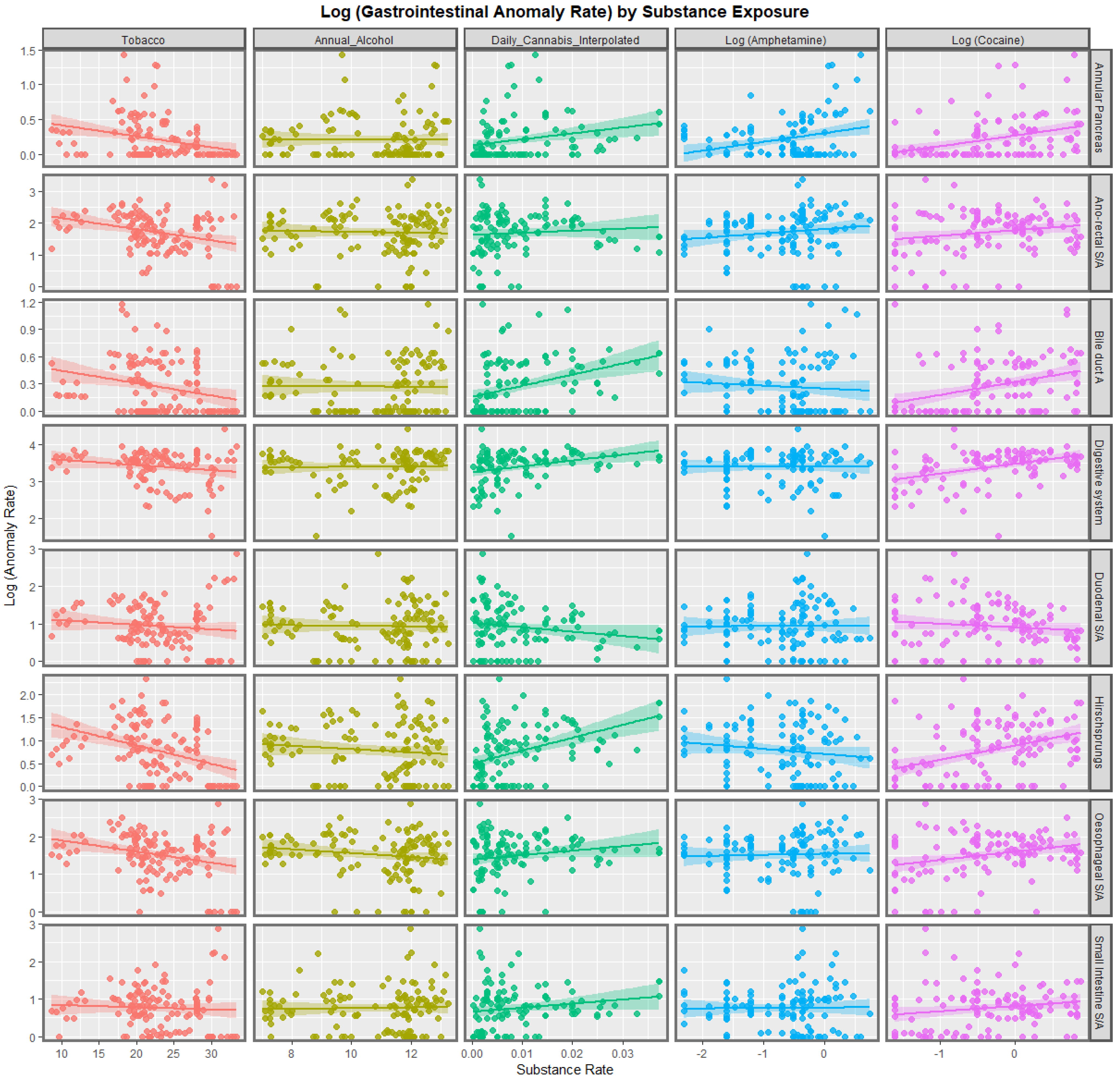
Figure 1 shows the relationship of the eight anomalies of interest with the various substances: tobacco, alcohol, daily cannabis use interpolated, amphetamine and cocaine. Interestingly, tobacco and alcohol do not appear to be strongly related to any of these CA’s. Amphetamine exposure does appear to be positively related to annular pancreas and anorectal stenosis or atresia. Cocaine appears to be significantly related to most of the anomalies on this list. Daily cannabis use appears to be positively related to annular pancreas, bile duct atresia, digestive system disorders and Hirschsprungs disease with weaker relationships with some other CA’s.
The correlation coefficients for this Figure are shown in Supplementary Figure S1 and Supplementary Table S4. Other than a close relationship between daily cannabis use and cocaine use, most of the correlations are weak-to-moderate. The significance levels of these correlations are shown quantitatively in Supplementary Table S5 and Supplementary Figure S2 and semi-quantitatively in Supplementary Figure S3.
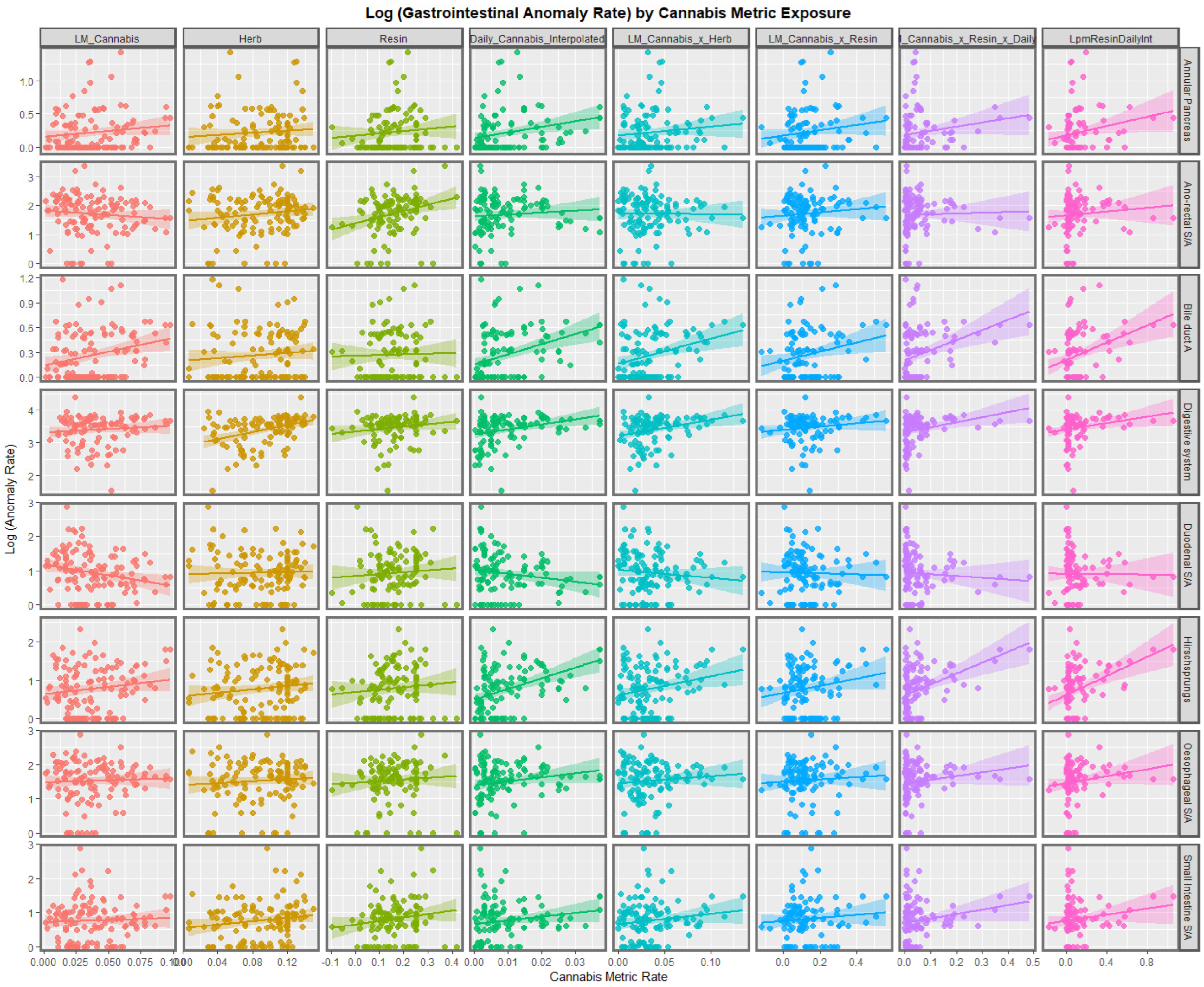
Figure 2 continues this graphical analysis by listing the various anomalies against the different metrics for cannabis exposure. The last month cannabis use appears to be positively related to bile duct atresia and Hirschsprungs disease. Cannabis herb THC concentration appears to be related to small intestinal stenosis or atresia. Cannabis resin THC concentration appears to be strongly related to anorectal stenosis or atresia and small intestinal stenosis or atresia. Daily cannabis use interpolated shows strong positive relationships with annular pancreas, bile duct atresia and Hirschsprungs disease. Many of the compound metrics derived from these primary covariates also show strong positive slopes, as indicated. Some of the regression lines for bile duct atresia and Hirschsprungs disorder appear to be particularly steep.
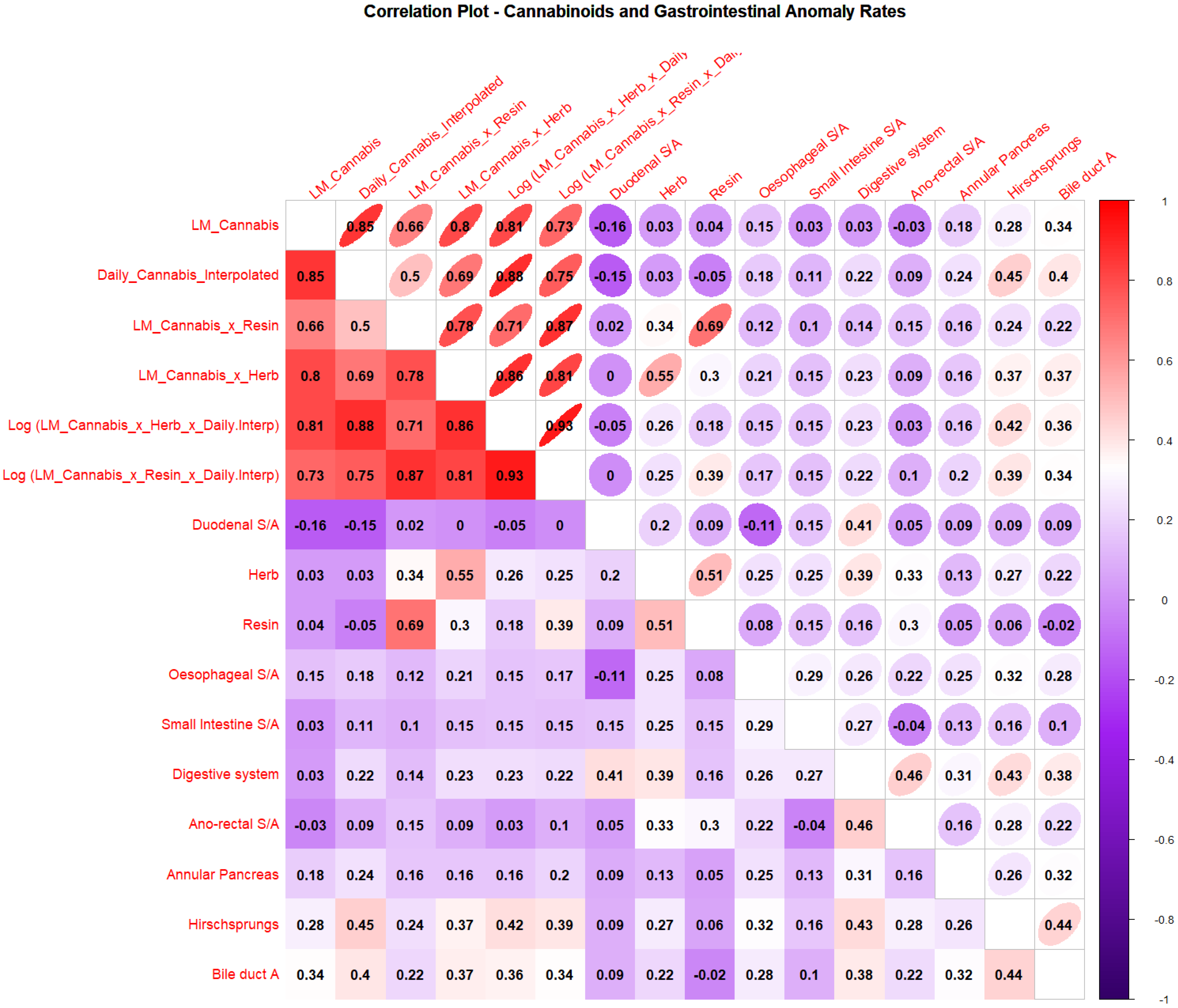
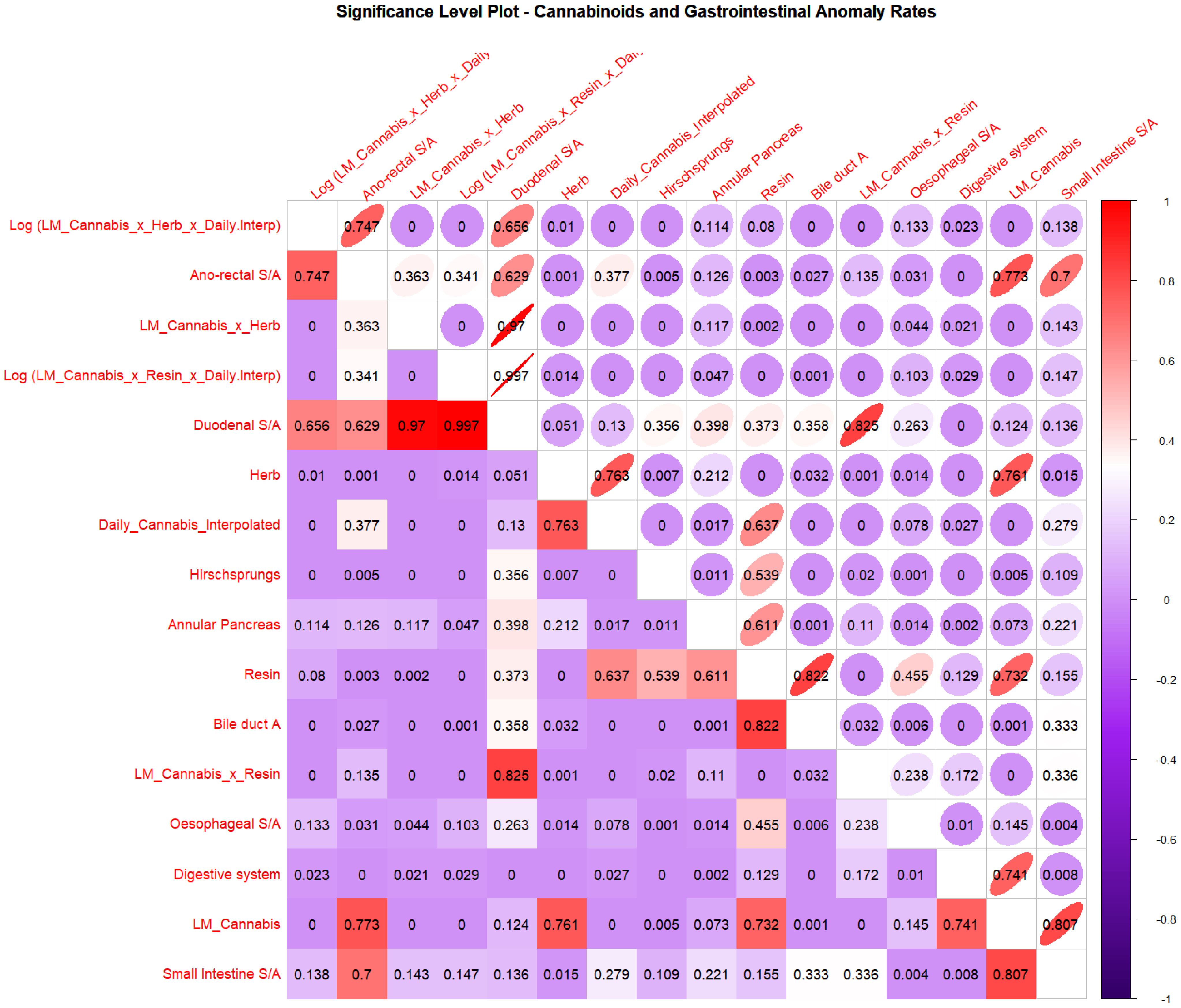
The correlations from this Figure are shown graphically in Figure 3 and listed in Supplementary Table S6. The significance levels of these correlations are shown quantitatively in Figure 4 and Supplementary Table S7 and semi-quantitatively in Supplementary Figure S4. It appears from these results that many of the congenital anomalies have moderate correlations with various cannabis metrics including bile duct atresia, oesophageal stenosis or atresia, digestive system anomalies, anorectal stenosis or atresia, Hirschsprungs disease, annular pancreas and duodenal stenosis or atresia, and small intestinal stenosis or atresia.
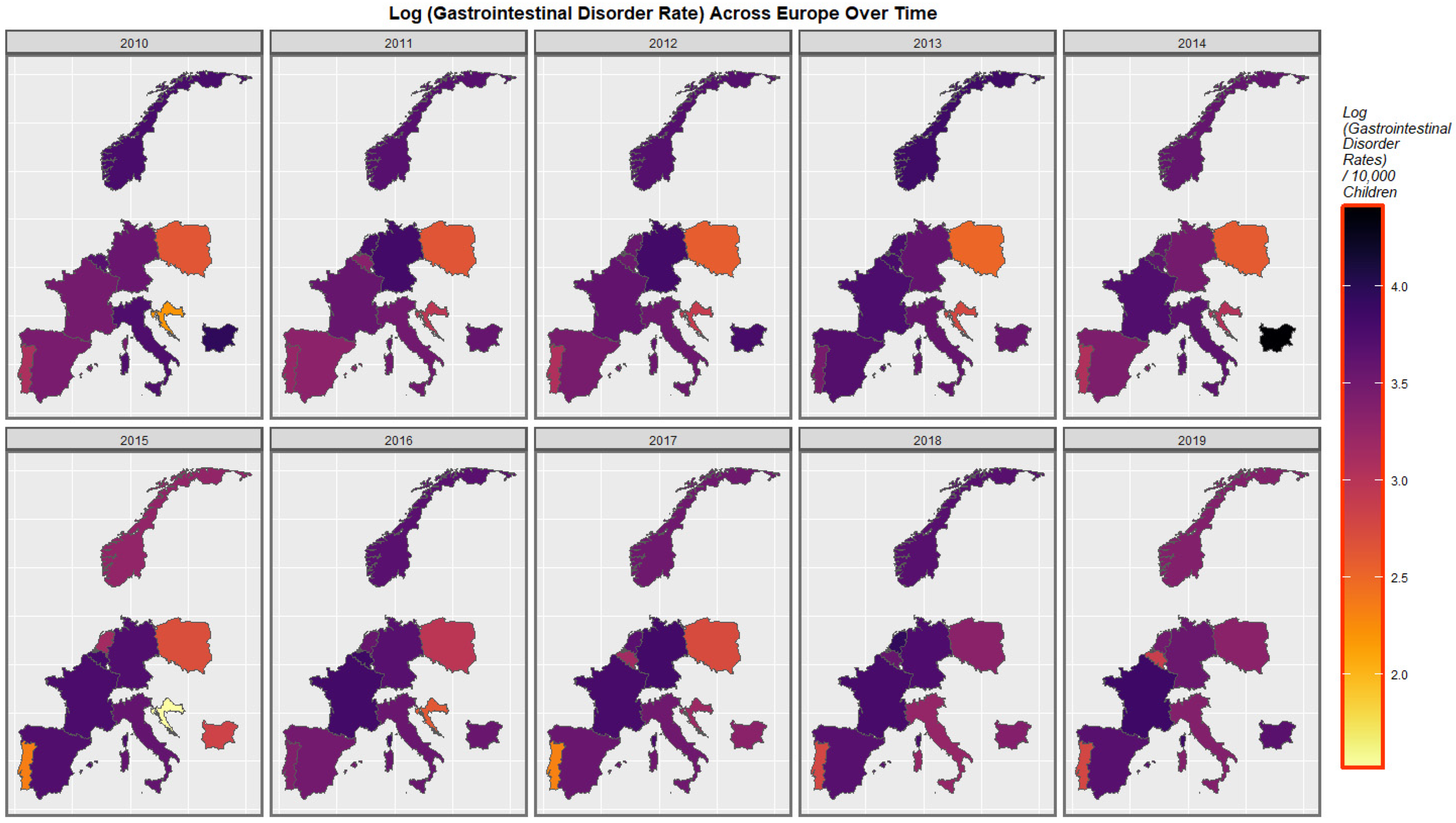
Figure 5 shows the rate of congenital gastrointestinal disorders across Europe over the last decade. As one reviews these maps, it is useful to keep in mind the nations which were noted to have high or rising daily use as described in the Section 2. Rates seem to have increased across the continent and particularly in France, Spain, Germany and Croatia. They have remained fixed and high in the Netherlands and Norway. It is noted that all of these nations are in the high or rising daily cannabis-use group.
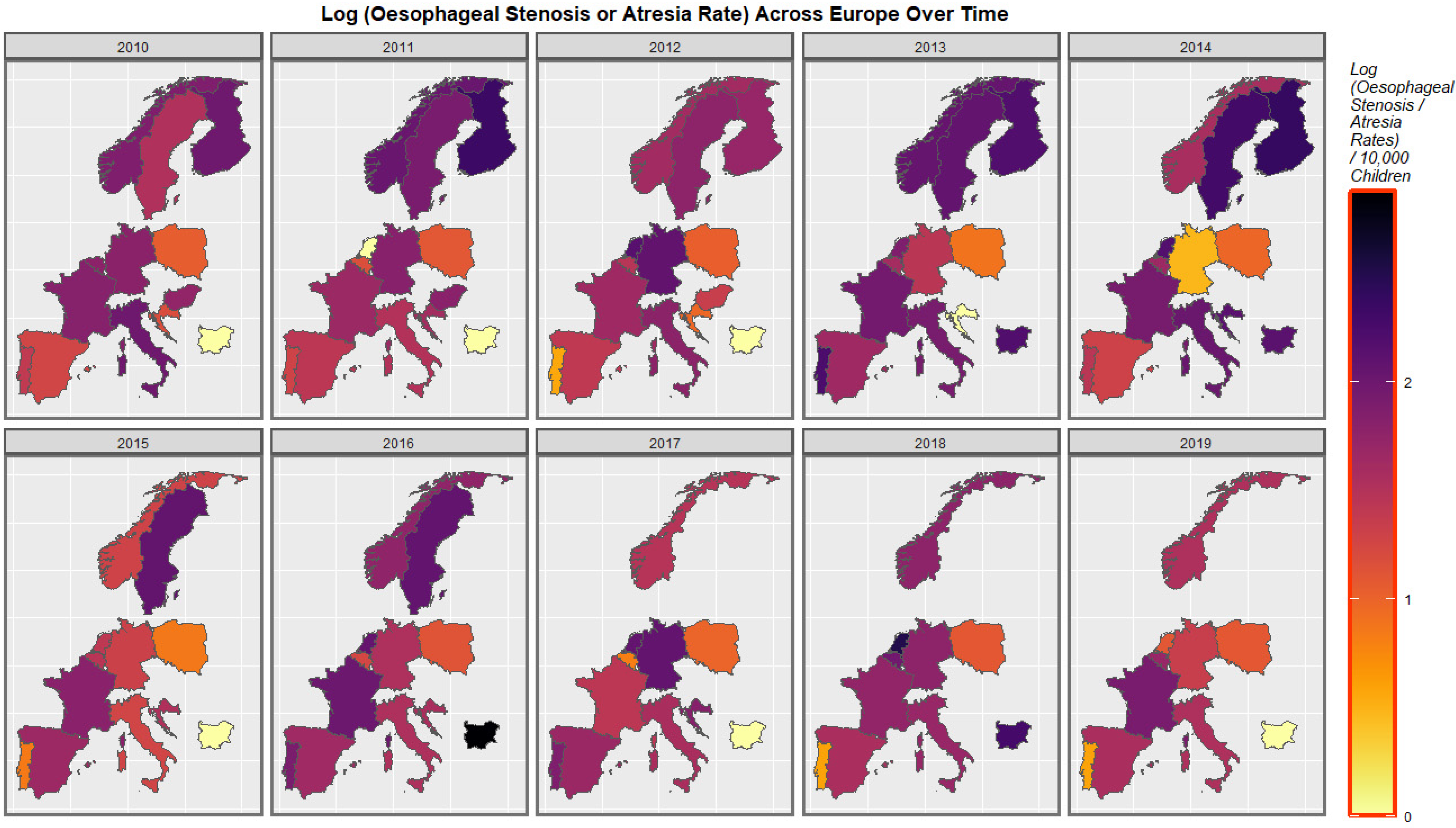
Figure 6 shows the rates of esophageal stenosis or atresia across Europe. Fluctuations in several countries are evident.
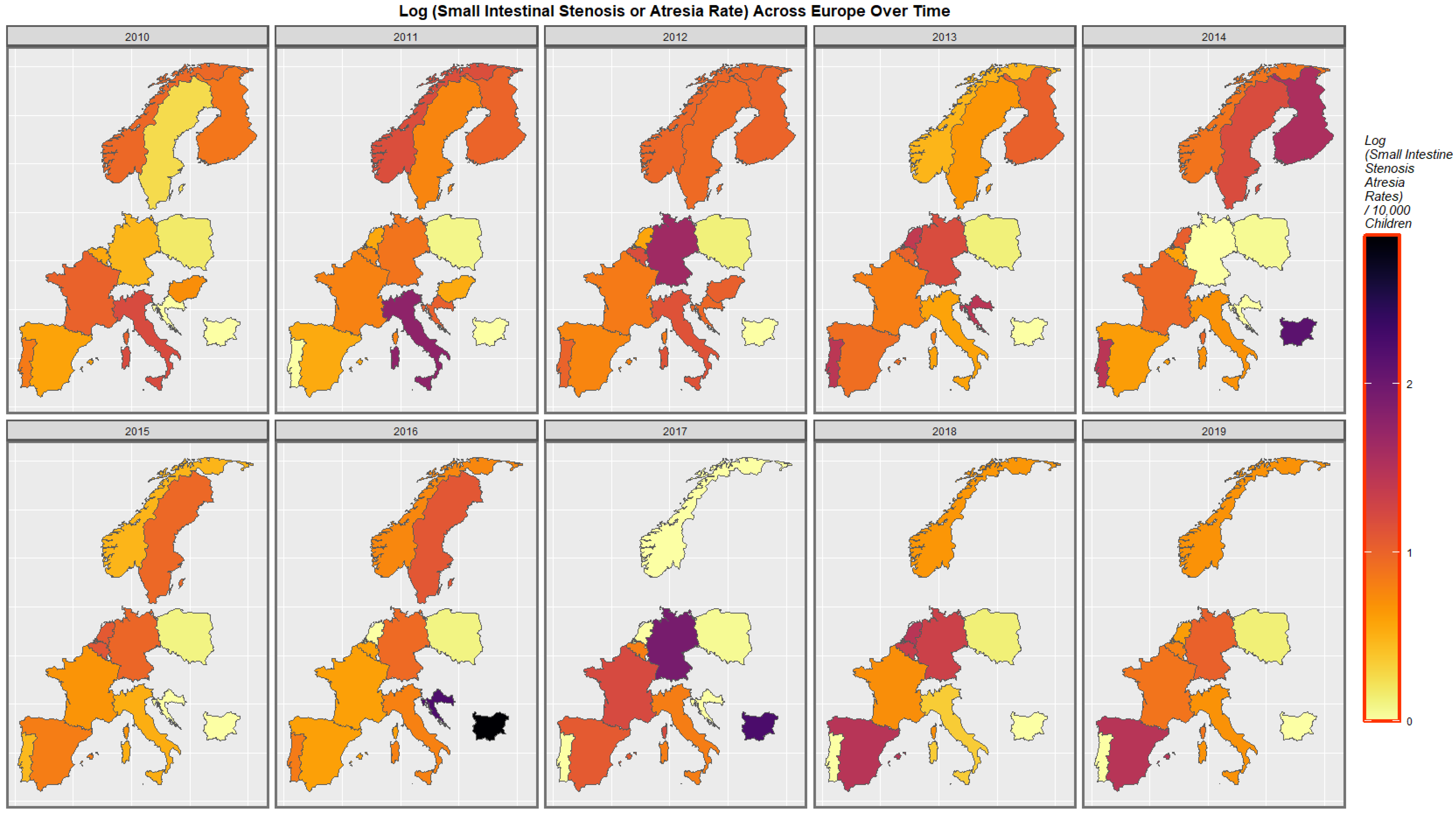
The rates of small intestinal stenosis or atresia are depicted in Figure 7. Increased rates in Spain, Croatia, Sweden, Germany and Bulgaria are apparent. The rates in Italy have declined. The rates in the low countries have fluctuated across this period.
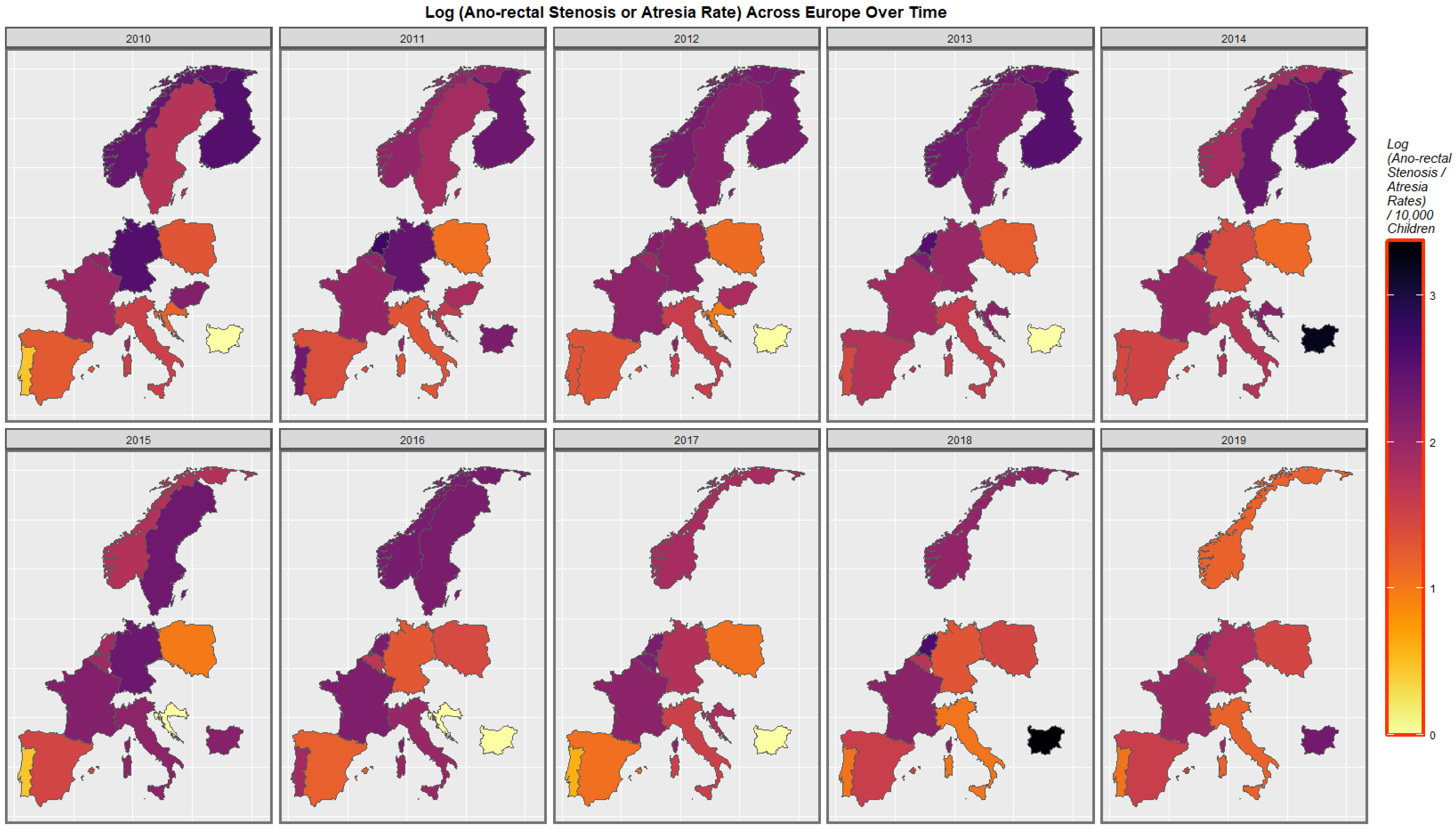
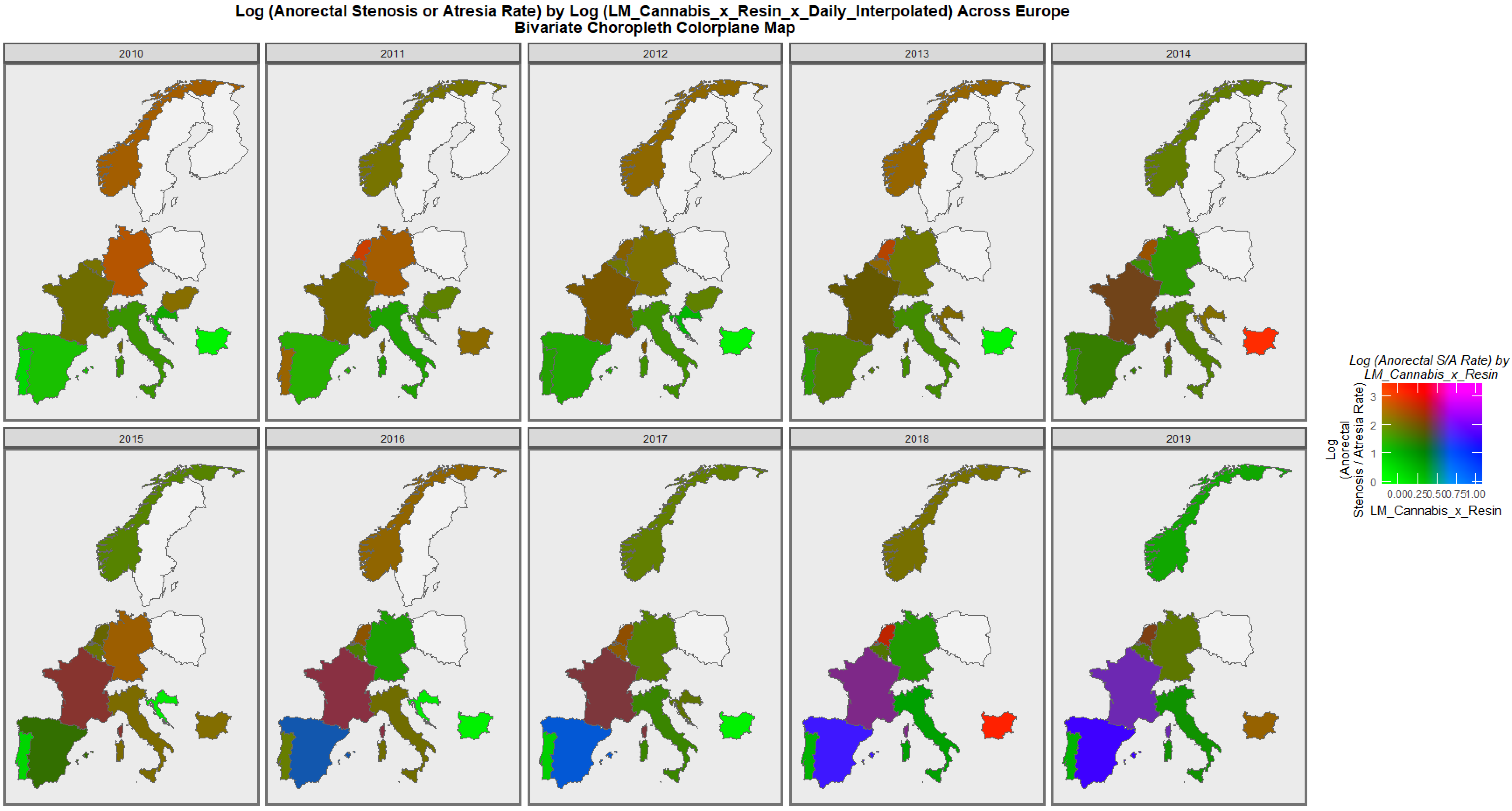
The rates of anorectal stenosis or atresia are illustrated in Figure 8. The rates are noted to have increased in Spain, Sweden, Poland and Bulgaria. The rates in the Netherlands were often high. The rates in Germany declined across this decade.
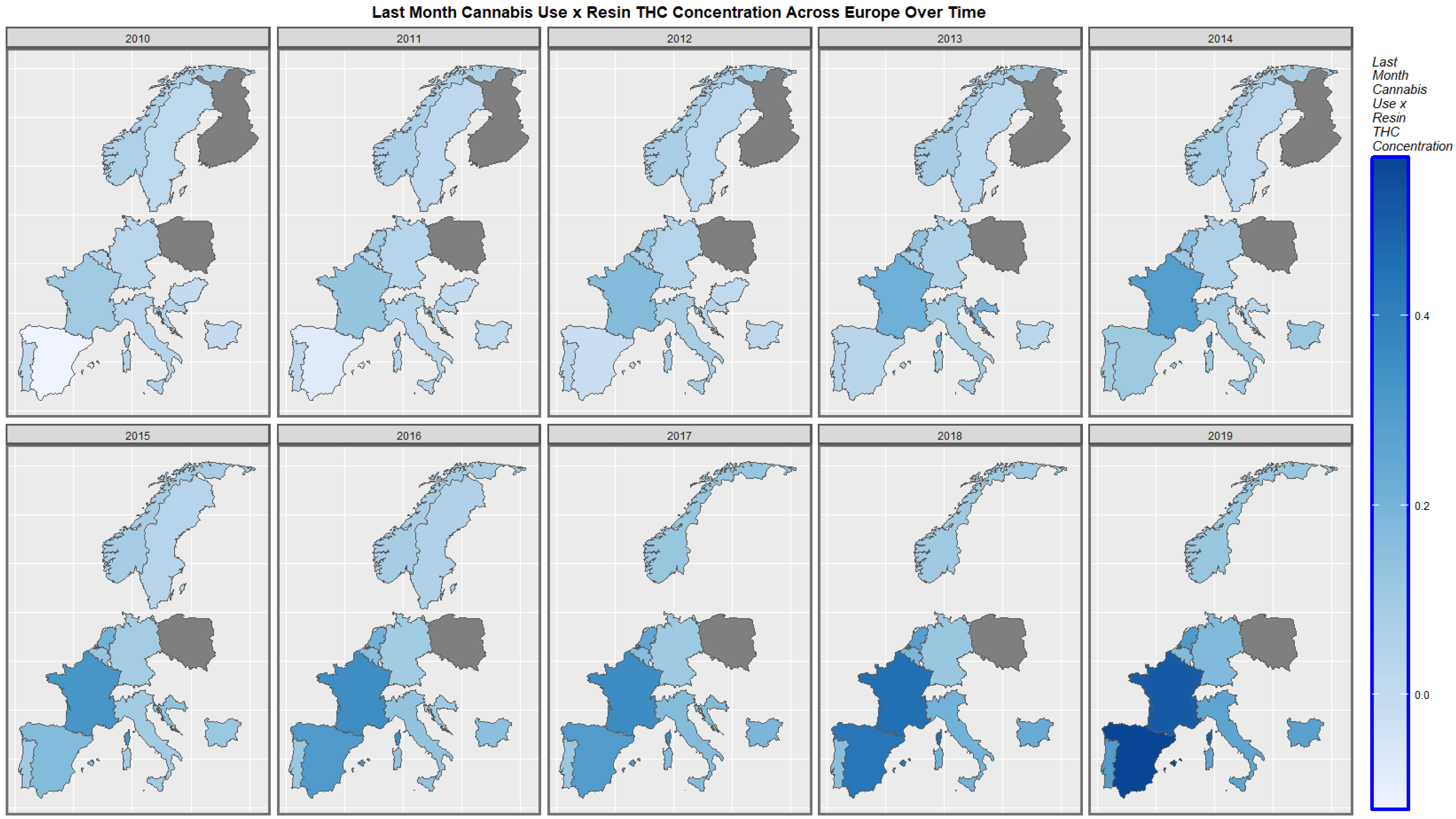
The rates of the compound cannabis metric, last month cannabis use: resin THC concentrations over time, are shown across Europe in Figure 9. The rates have increased in most places, with particularly marked rises in Spain, France and the Netherlands.
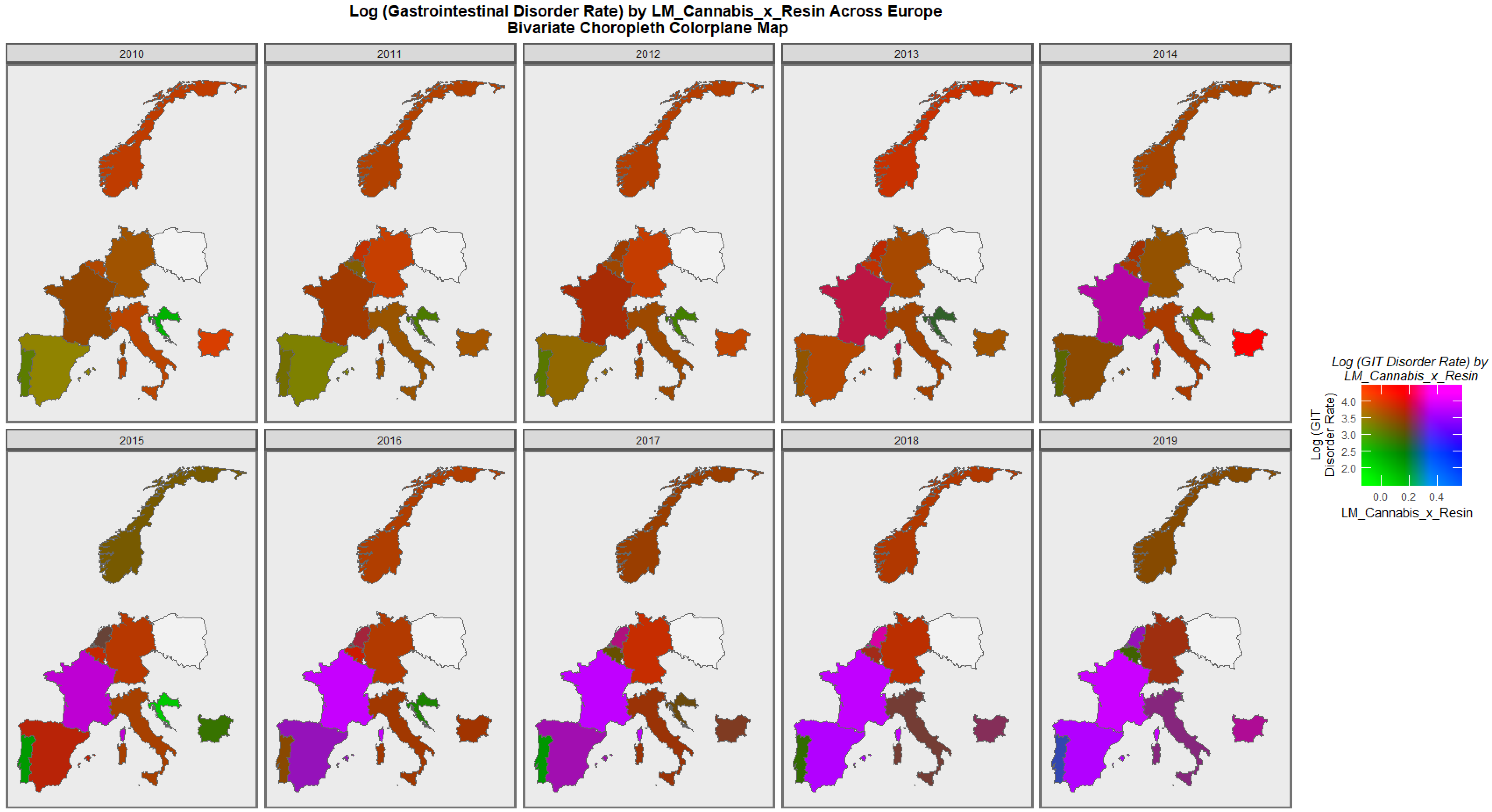
Figure 10 is a bivariate plot of the coincident rate of digestive system disorders and the compound cannabis-exposure metric of last month cannabis use: cannabis resin THC concentration. The plot is read by observing the areas which have turned pink or purple, which indicate simultaneously high rates of both covariates. Other colours have meanings, as shown in the colorplane key. Thus, the plot explains clearly the convergence of elevated rates of this cannabis-exposure metric and congenital digestive disorders over most of the continent including France, Spain, Bulgaria and the Netherlands. High rates in nations with rising daily cannabis use are clearly shown.
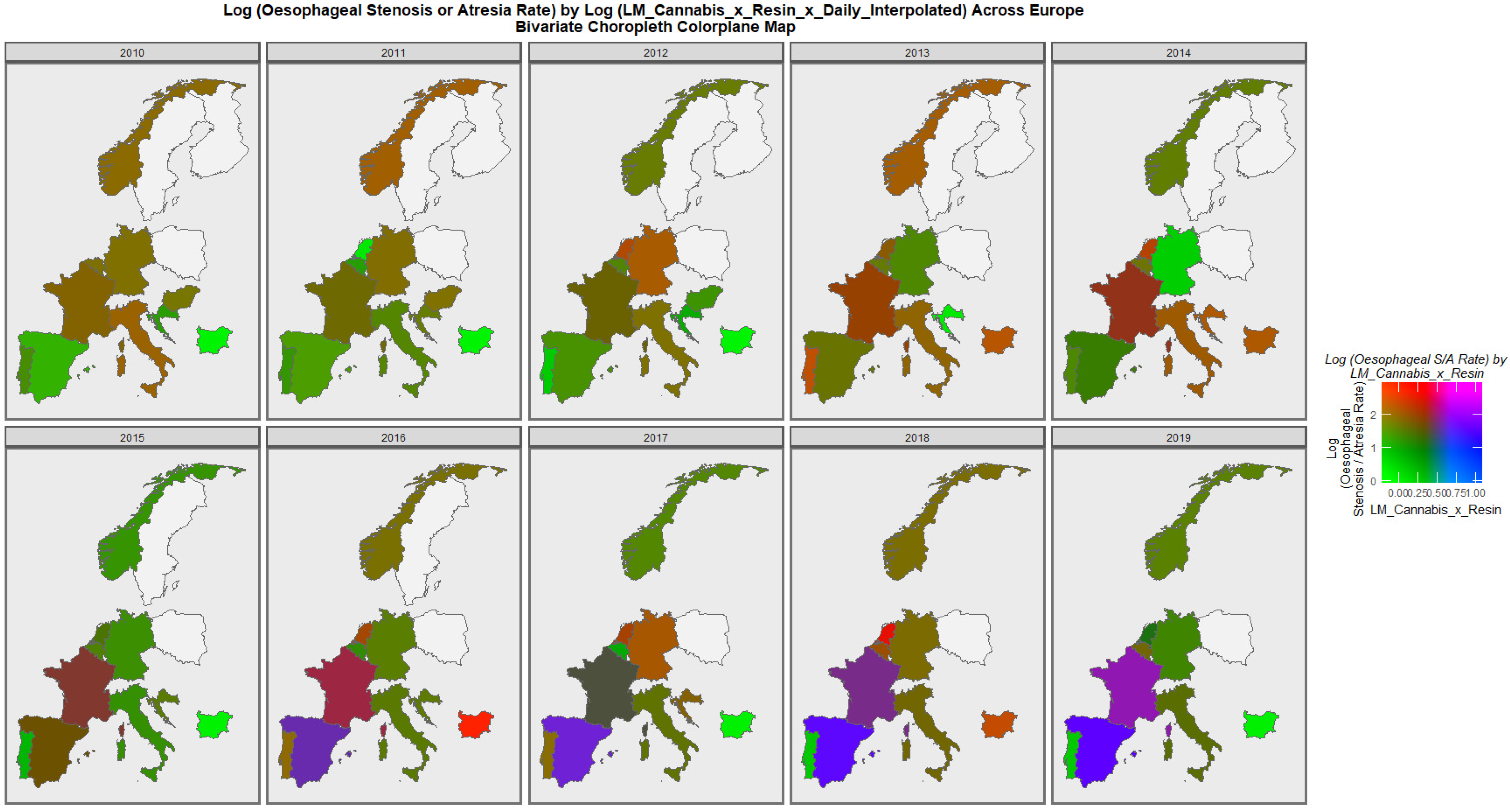
Figure 11 shows the rates of esophageal stenosis or atresia against the compound cannabis metric of last month cannabis use: cannabis resin THC concentration: daily cannabis use interpolated. The areas of land covered by Spain and France are noted to turn purple towards the end of the decade, indicating simultaneously elevated rates of both covariates.
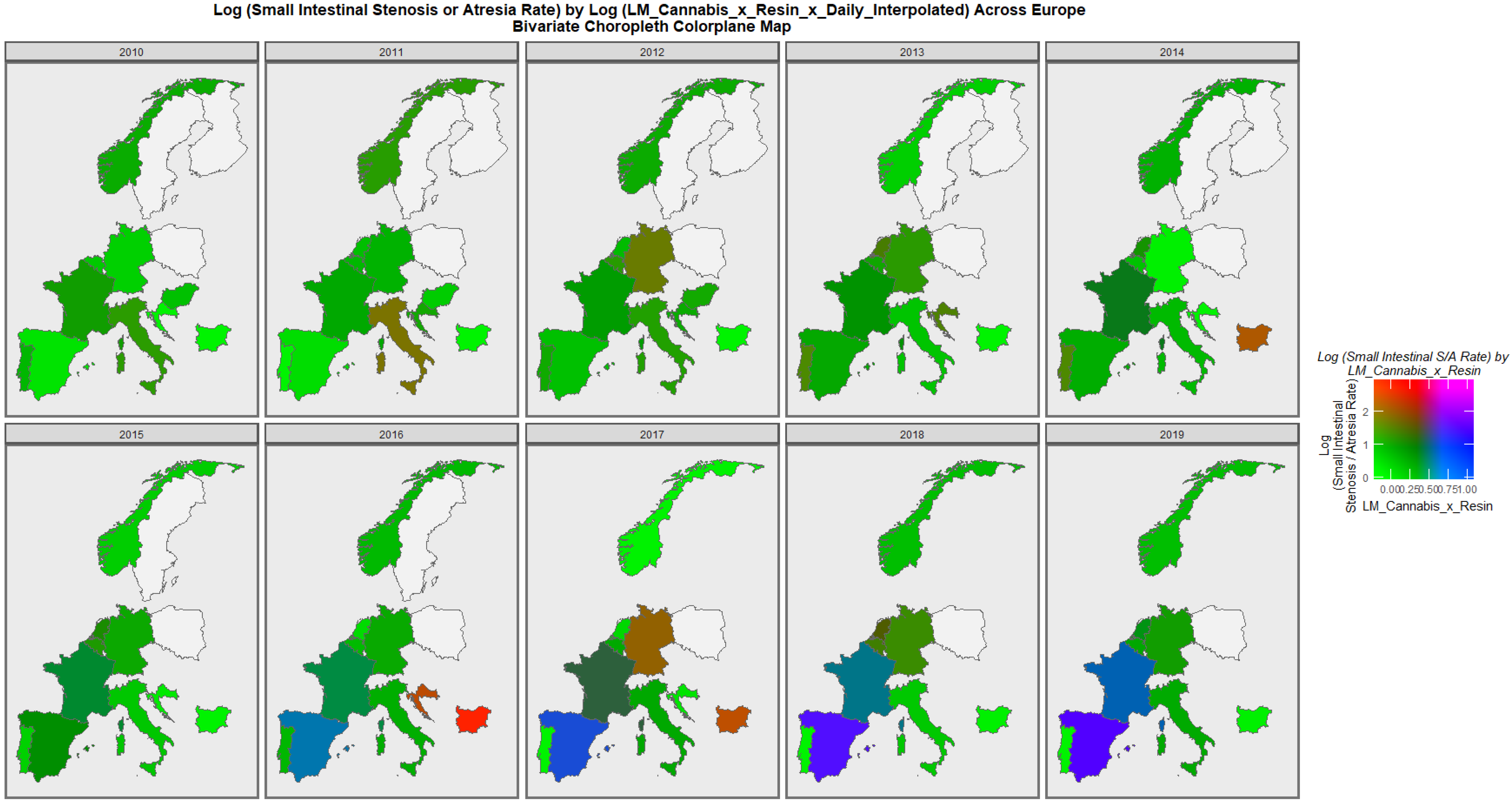
Figure 12 performs a similar exercise for small intestinal stenosis or atresia. Coincident elevations are not seen in this plot.
When a similar exercise was repeated for anorectal stenosis or atresia, the area of France was noted to have turned purple in the later years of this decade (Figure 13).
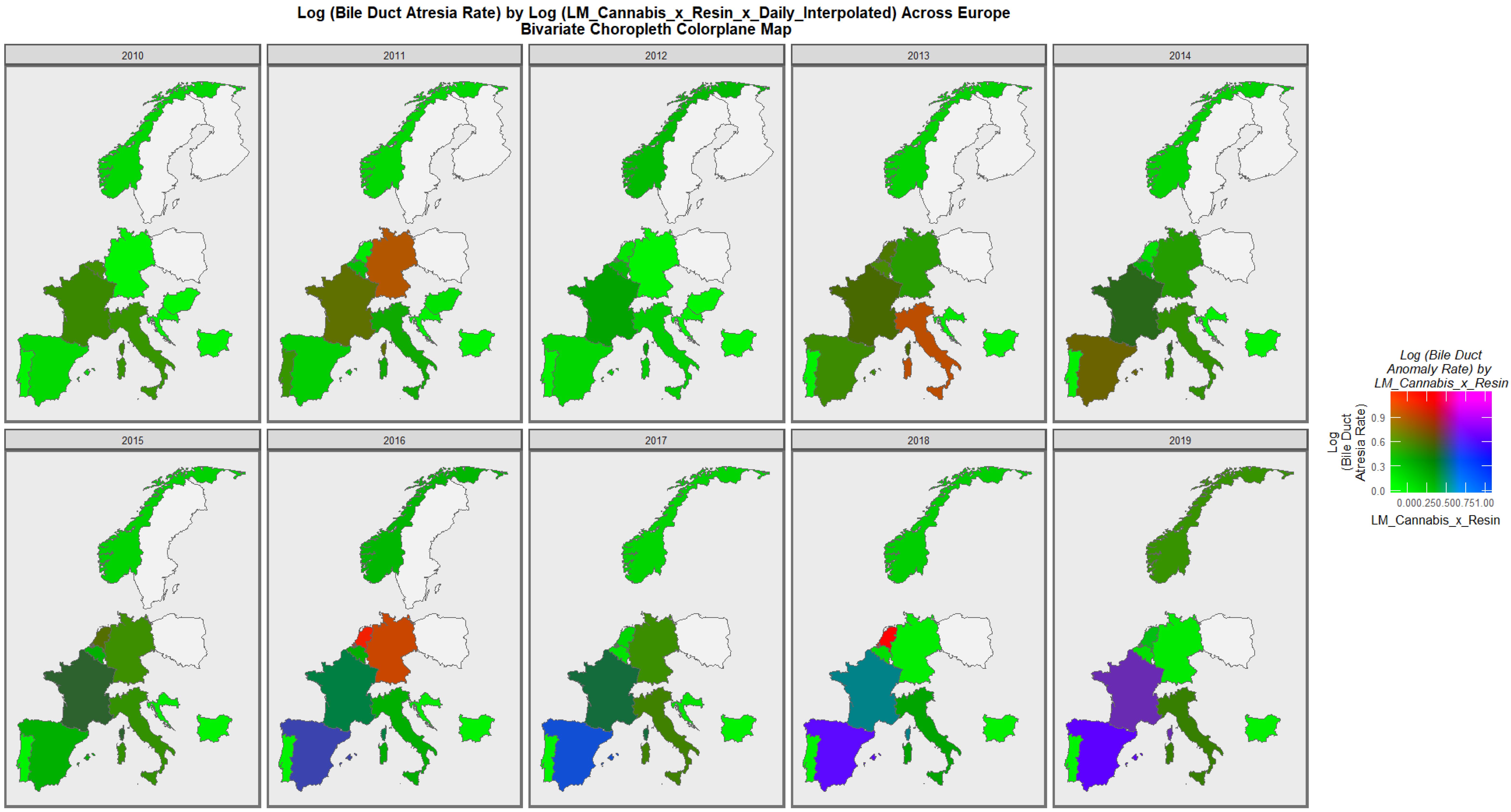
When bile duct atresia was considered along with last month cannabis resin THC concentration and daily use interpolated, the appearance shown in 
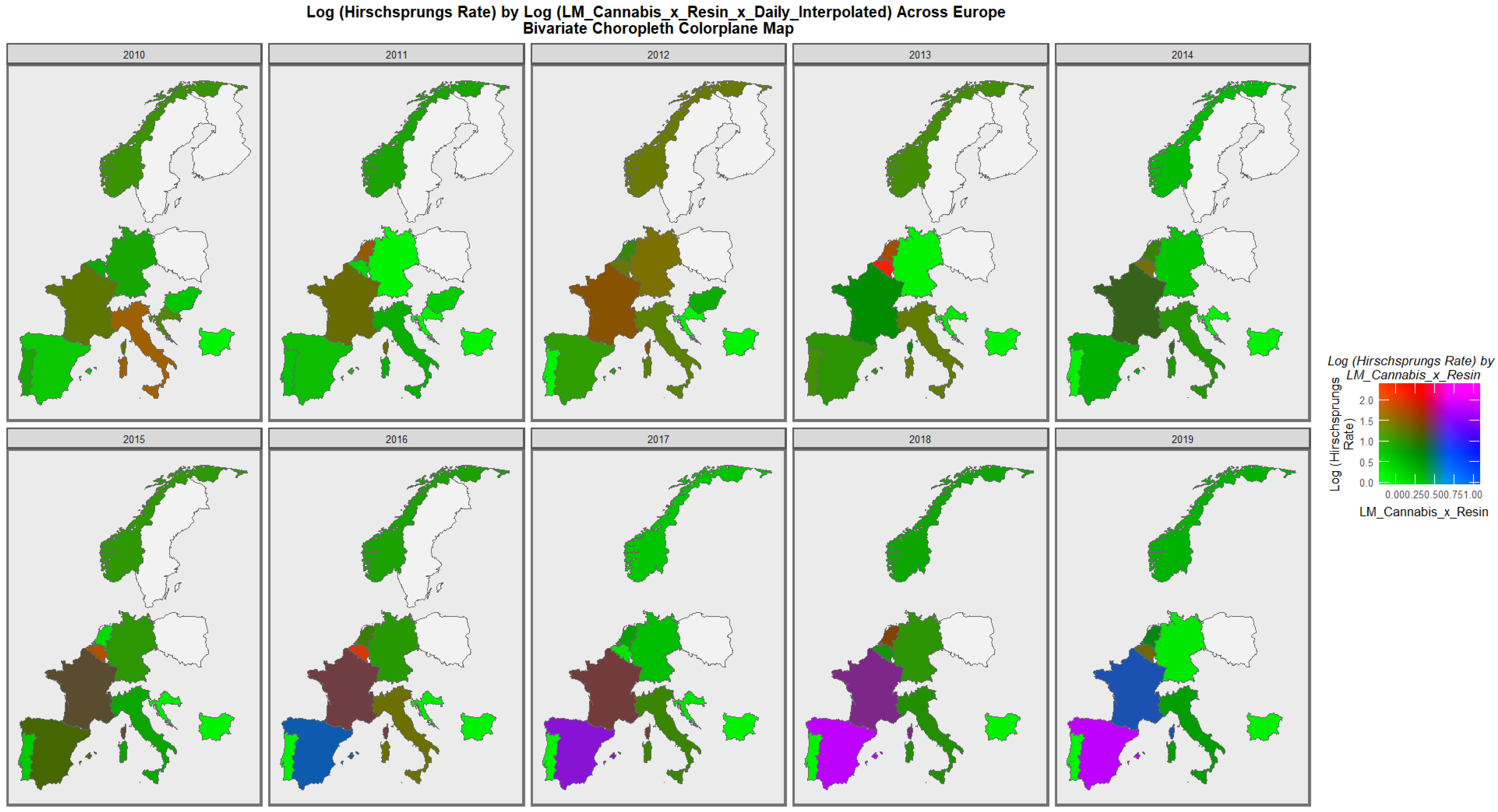
Figure 14 is seen. The clear emergence of confluent trends in Spain and France are evident. Similar trends are seen in Spain and France for Hirschsprungs disease, as shown in Figure 15.
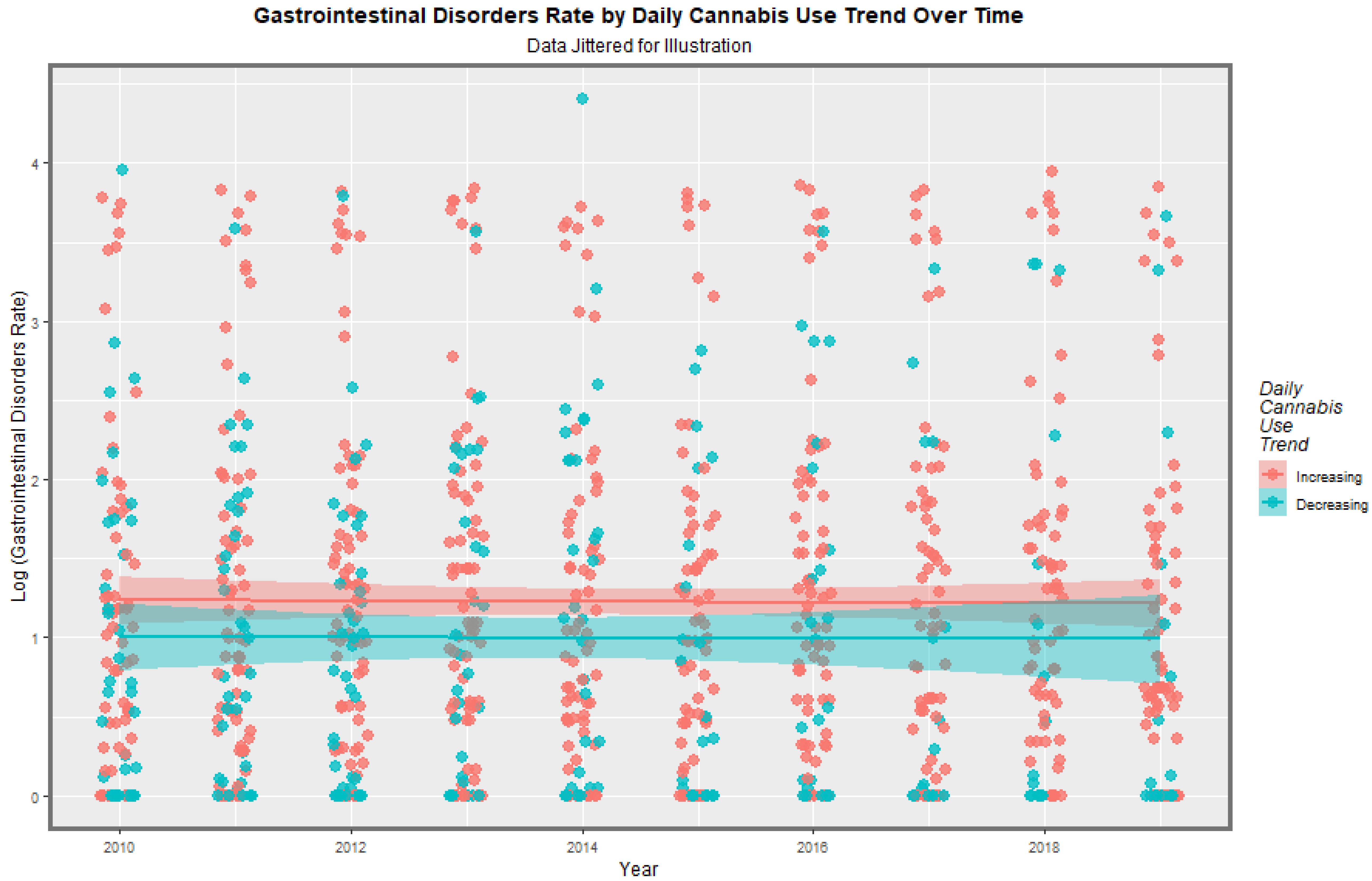
Based on recently published epidemiological reports, European nations were categorized as having either high and rising daily cannabis use or low and/or falling daily cannabis use in the last decade [6]. When all the CA’s are aggregated together, the appearances illustrated in Figure 16 are shown. Countries in which daily use is increasing have higher rates than those of low and/or falling daily cannabis use. This feature is confirmed at linear regression (β-est. = 0.2273, t = 1.959, p = 3.15 × 10⁻³; model Adj.R.Squ. = 0.0080, F = 8376, df = 1, 959, p = 0.0032). The E-values applicable to these effects are E-value estimate = 1.88 and minimum E-Value (mEVv) = 1.46.
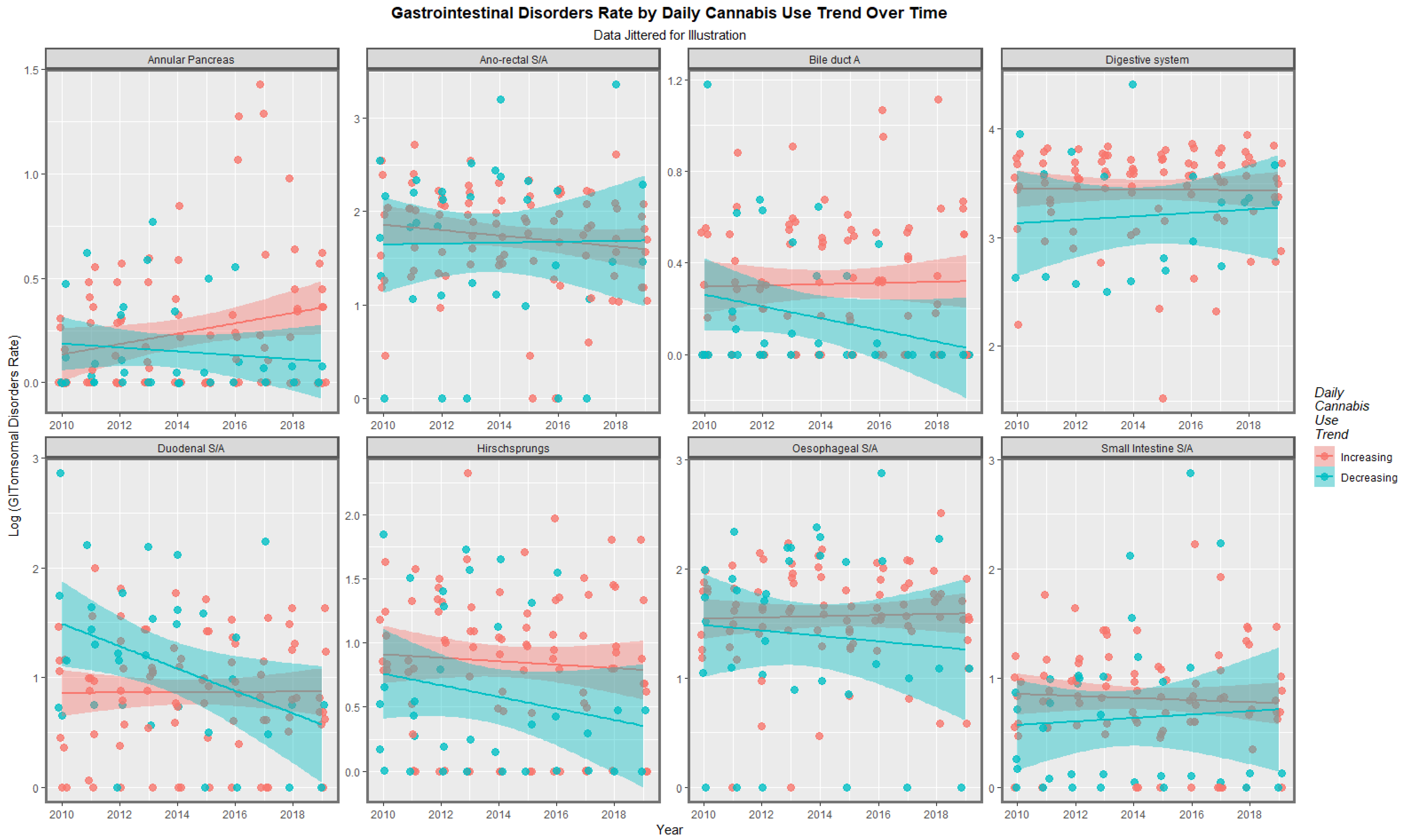
When this exercise was undertaken for each CA separately, the appearances disclosed in Figure 17 are found. It appears that for several CA’s, the nations with increasing daily use have higher digestive CA rates. This view was also established at mixed-effects regression (using the anomaly as the random effect; β-est. = 5.49 × 10⁻⁵, t = 2.909, p = 0.0037; model AIC = 1557.610, Log.Lik. = 158.935).
Supplementary Table S8 presents the 96 regression models implied from Figure 1 and Figure 2 along with their slopes, significance levels and E-values. The table is ordered by descending minimum E-values. It is of interest that daily cannabis use interpolated occupies the first entries in the table and that the highest anomalies listed are Hirschsprungs disease, bile duct atresia and digestive system disorders.
When the 26 models with positive regression coefficients and significant p-values are extracted from this list of models, Table 1 is obtained. The very high E-values reported here clearly imply that a causal relationship is in operation.
The next step in the analysis is to move into a multivariable framework where the importance of these various covariates can be compared. However, in the presence of 13 variables for substance exposure, it is most appropriate for use in the specific regressions.
This issue was directly addressed using random forest regression followed up with variable importance calculations to generate variable importance tables, of which are listed as Supplementary Tables S9–S13.
Five specific CA’s were chosen for detailed study for the reasons outlined in the Section 4.
Supplementary Table S14 presents several final inverse-probability-weighted-panel regression models for esophageal atresia (with or without tracheo-esophageal fistula) which are additive, interactive or temporally lagged, respectively. The inverse probability weighting is a technique of considerable importance in that it allows for the analysis to progress beyond a merely observational study into a pseudo-randomized theoretical conception from which causal inferences can be drawn. It is noted that in this table with additive and lagged models that various terms including cannabis metrics survive model reduction, and thus are significant after controlling for all other covariates, have positive regressions coefficients and are statistically highly significant (from p = 1.83 × 10⁻⁵).
Supplementary Tables S15–S18 continue this panel analysis for bile duct atresia, small intestinal stenosis or atresia, anorectal atresia and Hirschsprungs disease, as indicated. In each of these models, the metrics for cannabis exposure appear in the final models after model reduction and full adjustment, have positive regression coefficients and are highly statistically significant. The sole exception to this is bile duct atresia at two years of temporal lag.
The next issue relates to the performance of these models in a geospatial regression paradigm which appropriately and adequately controls for methodological issues such as random error effects, serial autocorrelation, spatial correlation and spatial autocorrelation in the data.
Supplementary Figure S5 shows the initial, adjusted and finished geospatial international links which were calculated and modified and used to form the spatial weightings which were employed in the geospatial regression modelling. The figure represents in a map-graphical format that the spatial relationships which are digitized in a sparse matrix form to generate the spatial weight matrix used in the geospatial regression equations.
Table 2 shows the final geo-spatiotemporal models for additive, interactive and temporally lagged models for esophageal atresia. The terms for cannabis exposure appear in the model lagged to two years.
For bile duct atresia, no cannabis terms remain in the final models (Table 3). However, this may be an artefactual issue related to the fact that 49 of the 110 values were at zero, which is likely a coding artefact. As a result, the error structure of these models was constrained to be an ordinary least squares error structure which is a less sensitive analytical framework.
Geospatial models for small intestinal stenosis or atresia (SISA) and anorectal stenosis or atresia are presented in Table 4 and Table 5. In all of the models, listed terms incorporating cannabis metrics appear in the final models after full adjustment, have positive coefficients, are overwhelmingly positive and are highly statistically significant.
The Hirschsprungs disease dataset was also grossly incomplete with 30 values of the total 110 values set at zero, which was clearly a coding artefact. Data for Croatia, Bulgaria, Germany, the Netherlands, Portugal and Belgium were completed by mean substitution for each country. For Bulgaria, all data were absent, so the data were set at the overall mean of the total sample (0.932/10,000 births). When these adjustments were made for data imputation, the pattern seen for SISA and anorectal stenosis or atresia was confirmed in this dataset when adjustments for serial correlation were incorporated into the error structure of the models (Table 6).
E-values are applicable to each of the multivariable models presented. E-values for panel models are presented in Table 7 and for geospatial models in Table 8. Table 9 lists all 35 together in descending order of the minimum E-value. It is noted that Hirschsprungs disease, SISA and anorectal stenosis or atresia head up the list of anomalies in this table, and the first 10 all relate to daily cannabis exposure. However, the results relating to Hirschsprungs disease should be interpreted with some caution in view of the large number of missing data in this dataset.
In Table 10, these 35 E-values are listed in descending order of mEVv. From this Table, it is apparent that 25/35 (71.4%) of E-value estimates exceed 9 and are, therefore, in the high zone [89], and all 35 (100%) exceed the threshold for causality of 1.25 [88]. For the list of mEVv’s, 19/35 (54.3%) exceed nine and are in the high zone, and 34/35 (97.1%) exceed the 1.25 threshold for causality.
E-values may be listed in order of the anomaly concerned and this listing is shown in Table 11. Summary data for these E-value results are shown by anomaly in Table 12 where they are also listed in descending order of median mEVv. Hirschsprungs disease and esophageal stenosis and atresia are noted to move up this table and have high median E-value estimates and median mEVv’s.
Table 9 can also be listed in order of the independent variable term. This is shown in Table 13. These terms may be grouped by the major primary cannabis-related variable of interest, which is, respectively, daily use, or the THC concentration of cannabis resin or herb. This assignment is coded in as the new added “Group” column in this table. Table 14 summarizes the selected descriptive statistics from this group and again lists the regression terms in descending order of the mEVv. Daily use moves up this table ahead of herb THC concentration and resin THC concentrations.
These data may be formally compared using Wilcoxon tests with results, as indicated in Table 15. From this table, it is apparent that the statistical comparisons between daily use and both herb and resin THC concentration are significant for both the estimate of the E-value itself and the mEVv, but the comparisons between herb and resin did not achieve statistical significance.
When interpreting these results, it is important to bear in mind the above-cited shortcoming with the many absent data points, particularly in the Hirschsprungs and bile duct atresia datasets.

4. Discussion

4.1. Main Results

The main result of this study was that seven gastrointestinal CA’s (GCA’s) were significantly related on either bivariate or multivariable testing to different measurements of cannabis consumption. The GCA’s identified at bivariate analysis were bile duct atresia, Hirschsprungs disease, digestive system disorders, annular pancreas and anorectal stenosis or atresia. The two additional GCA’s which were shown to be cannabis-related on the multivariable analysis were esophageal stenosis or atresia and small intestinal stenosis or atresia. Hence, the results from this large and versatile dataset confirmed the findings of other recent published series from many places [3,4,5,57,91]. Two new disorders were added to the list which has previously been described (see Introduction), namely, annular pancreas and digestive system disorders generally.
Tobacco and alcohol were not strongly related to any of these CA’s. Amphetamine exposure was positively related to annular pancreas and anorectal stenosis or atresia, and cocaine was significantly related to most of the anomalies.
Interestingly, a companion paper to the present paper was recently published and showed that VACTERL syndrome (vertebral, anorectal, cardiac, tracheo-esophageal fistulae/esophageal atresia, renal and limb anomalies) was strongly and causally linked with European cannabinoid exposure [57,92]. In that esophageal atresia is part of the VACTERL syndrome this finding provides evidence from this other reference, confirming the present findings reported herein.

4.2. Main Results in Detail

In the bivariate analysis, it was shown that the relationships of tobacco and alcohol to GCA’s were very weak or negative. The relationship of bile duct atresia with last month cannabis use was strong positive. The relationship of digestive system anomalies with cannabis herb was strong positive. The relationship of anorectal atresia with cannabis resin THC concentration was strong positive. The relationship of daily cannabis use with bile duct atresia and Hirschsprungs disease was strong positive.
Bivariate maps were considered. When the relationship between gastrointestinal disorders and last month cannabis use x cannabis resin THC was considered, both variables were noted to increase together in the Netherlands, France, Spain, Italy and Bulgaria (Figure 10). When the bivariate relationship of esophageal stenosis or atresia to last month cannabis use x cannabis resin THC concentration x daily cannabis use interpolated was considered, both covariates were noted to increase together in Spain and France (Figure 11). When the bivariate relationship of large intestinal stenosis or atresia to last month cannabis use x cannabis resin THC concentration x daily cannabis use interpolated was considered, both covariates were noted to increase together in France (Figure 13).
When countries with featured higher daily cannabis exposure were compared with countries which were not, the overall rate of GCA’s was higher in the former group when considered overall (p = 0.0032) and when considered on a by GCA basis (p = 0.0037).
In the bivariate analysis, five GCA’s were related to metrics of cannabis exposure ordered by median mEVv bile duct atresia (12.5), Hirschsprungs (9.27), digestive disorders (5.48), annular pancreas (1.67) and anorectal stenosis or atresia (1.18) (Table 1).
When the sequence of GCA’s was considered by inverse-probability-weighted-panel modelling, as follows, they were noted to be significantly linked with cannabis metrics, as indicated: esophageal stenosis or atresia, bile duct atresia, small intestinal stenosis or atresia, anorectal stenosis or atresia, Hirschsprungs disease: 1.83 × 10⁻⁵, 0.0046, 3.55 × 10⁻¹², 7.35 × 10⁻⁶ and 2.00 × 10⁻¹², respectively. When the same series of anomalies was considered in geospatial modelling, they were significantly cannabis-related from 0.0003, N.S., 0.0086, 6.652 × 10⁻⁵, 0.0002.
A total of 25/35 (71.4%) E-value estimates and 19/35 54.3% minimum E-values (mEVv’s) exceeded 9.0, and therefore, were in the higher zones [89]. A total of 100% E-value estimates and 97.1% mEVv’s were greater than 1.25, which is said to be the cut-off limit for causality [88]. The order of cannabis sensitivity by median mEVv was Hirschsprungs > esophageal atresia > small intestinal atresia > anorectal atresia > bile duct atresia.
It was fascinating to us that the top position in Table 1, which lists the significant bivariate regression coefficients, was taken by Hirschsprungs disease, confirming a recent report from the USA, especially in view of the finding detailed below that cannabis dependence is characterized by differential DNA methylation affecting three genes (GDNF, KIF26A and PSAP) which control enteric ganglion formation (supplementary material Page 308, p = 0.000274).
As noted, there were some shortcomings in the GCA rates. In the Hirschsprungs dataset, 30/122 (24.6%) zeros were replaced by mean substitution to allow for the analysis to proceed. In the biliary atresia dataset, 49/122 (40.2%) of the GCA rates were zero and were not able to be meaningfully substituted. These limitations of the data must be kept in mind when interpreting the present results.

4.3. Choice of Anomalies

The anomalies chosen for further study were selected because they had been identified in previous published series and/or they demonstrated strong signals in the bivariate analysis (Figure 2).

4.4. Qualitative Causal Inference

The Hill criteria [93] are accepted criteria for determining when an association may be considered to be causal in nature. Nine criteria are listed, including strength of association, consistency amongst studies, specificity, temporality, coherence with known data, biological plausibility, biological dose–response curve, analogy with similar situations and experimental confirmation. All of these criteria are fulfilled by the five GCA’s positively identified in this study which have previously been described in this literature. We would be inclined to accept the two which have not been previously described based on the external validity of the other results with the published literature overall and described in this report.

4.5. Quantitative Causal Inference

This study has employed two key tools of formal quantitative causal analysis. The first one, inverse probability weighting, answers the common criticism of observational studies—that the various experimental groups are not comparable across the population. Inverse probability weighting is the technique of choice to address this issue and it was applied to all the panel regression multivariable models presented. Its effect is to transform the analysis from a mere observational study into a pseudo-randomized study from which causal inferences may properly be drawn.
A second major criticism of observational studies is that they may be subject to uncontrolled confounding and that the apparently casual effect they report may in fact be due to some extraneous external covariate which has not been controlled. E-values (or expected values) are used to set quantitative constraints on this hypothetical external confounder by determining the degree of association required of it with both the exposure of concern and the outcome of interest. E-values over 9.0 are described as being in the high zone [89] and values greater than 1.25 are generally said to be required to attribute to causation [88]. The tobacco–lung cancer relationship has an E-value of nine, so this datum provides some appreciation of the real world meaning of these numbers. E-values also have confidence intervals. The 95% lower confidence interval is of particular interest in this context as it demonstrates quantitatively the confidence which can be had that the E-value estimate is different from unity. Therefore, the generally elevated E-value estimates reported in the present study are 71.4% in the very elevated zone, thus providing confidence regarding the robustness of these results.

4.6. Biological Mechanisms

Because pathophysiological mechanisms are central to the argument for causality, it is worthwhile considering a few of the mechanisms which have been described in some detail. Thus, these findings from the basic laboratory sciences are germane and become central to the present epidemiological discussion.

4.7. Cannabinoid Inhibition of Morphogens

It is important to appreciate that embryonic patterning and morphogenesis happens largely under the control, guidance and specification of gradients of various tissue morphogens. Many of the key morphogens are disrupted by cannabinoids including bone morphogenetic proteins [94,95,96], fibroblast growth factor [97,98], sonic hedgehog [99] and retinoic acid [100,101,102]. This may occur either directly or via epigenomic means, especially in the case of sonic hedgehog.

4.8. Epigenomic Control of Gastrointestinal Morphogenesis

A fascinating serial epigenomic study from Schrott and colleagues was recently published, which is packed with important information pertinent to the present discussion and is, therefore, worth exploring in some detail [25]. The researchers compared epigenome-wide DNA methylation patterns in human and rat sperm both in cannabis dependence and eleven weeks later in cannabis withdrawal. The period of one human sperm cycle is 11 weeks. Comparisons were made both between groups and over time within subjects.
In the body of their report, investigators noted from functional annotations from Ingenuity Pathway Analysis that pathways relating to growth of an organism, liver lesions and agenesis were differentially methylated regions (DMR’s). During cannabis withdrawal, the featured annotations included organismal death.
The researchers also published a 359-page supplementary appendix providing further details of these findings. Remarkably, there were 112 functional annotations pertaining to gastrointestinal disease. Clearly, there is too many to describe in detail, but by the way of example, one such finding noted 333 genes involved in cannabis dependence in gastrointestinal tumours (page 253, p = 1.02 × 10⁻¹⁵).
There were nine annotations relating to esophageal lesions (e.g., 31 genes, page 324; 16 genes, page 348).
We were not able to identify any annotations for the small intestine.
Many annotations were identified for the large intestines, including malignant large intestinal neoplasm (306 genes p = 7.65 × 10⁻¹⁵ in cannabis dependence, page 257; 258 genes, page 258, p = 1.11 × 10⁻¹⁴; 314 genes, p = 6.00 × 10⁻¹⁴, page 260, cannabis dependence; 313 genes, p = 7.15 × 10⁻¹⁴ page 261; 120 genes, p = 7.45 × 10⁻⁶, page 326, cannabis withdrawal; 122 genes 6.79 × 10⁻⁵, page 331 cannabis withdrawal; and 121 genes, page 333, p = 0.000108 in cannabis withdrawal).
Gastrointestinal tumour was also noted (74 genes, p = 3.42 × 10⁻⁵, pages 328; 121 genes, p = 3.56 × 10⁻⁵, cannabis withdrawal).
In view of the strong signal detected in this study for Hirschsprungs disease, which was concordant with other studies [5], it was fascinating that three genes were identified controlling the enteric ganglion formation (GDNF, KIF26A and PSAP, page 308, p = 0.000274).
There were two hits for hepatobiliary carcinoma (176 genes, page 284, cannabis dependence; and 179 genes, page 286). Pancreatobiliary tumour was also identified (24 genes, page 288, cannabis dependence).
Pathways in pancreatic disease were also identified in pancreatic cancer (95 genes, p = 1.19 × 10⁻⁵, page 297 in cannabis dependence; 106 genes, page 298; and 90 genes, page 299; 85 genes page 300).
From this brief survey, it is clear that epigenomic signals can effectively explain many of the epidemiological findings in the present report.

4.9. Generalizability

Since this dataset utilizes one of the largest and most comprehensive CA datasets in the world, the data are inherently robust. We have also used advanced modelling techniques such as inverse probability weighting, random Forrest regression and geotemporospatial regression to further explore using multivariable adjustment relationships which appeared to be robust at bivariate regression. The study as a whole uses the formal quantitative techniques of causal inferential modelling throughout so that the analytical paradigm within which we are working transitions from the merely observational to the pseudorandomized environment from which it is quite appropriate to draw causal conclusions. Since our study demonstrates causal effects and is consistent with other reports in the world literature, these results are likely to be broadly generalizable with the sole caveat that the results reported for Hirschsprungs disease and biliary atresia likely represent lower bounds on the real effects due to the limitations of these particular datasets.

4.10. Strengths and Limitations

This study had a number of strengths and limitations. Its strengths included using one of the largest and most comprehensive CA datasets in the world and the use of advanced causal inferential modelling techniques, particularly inverse probability weighting and E-values, along with geospatiotemporal regression. We have also used maps to illustrate many key trends, including bivariate maps which allow for the clear and explicit display of bivariate simultaneous trends. We used random forest regression for the covariate selection, which adds discipline and rigour to this complex process. The study’s limitations include the unavailability of individual exposure data to the study’s investigators, of which is a limitation shared by many epidemiological studies. Some exposure data were missing and had to be completed by linear interpolation. This applied especially to the daily exposure data. The quality of some of the GCA data was also questionable. As noted, 24.6% of the Hirschsprungs disease rates were reported as zeros and were replaced by mean substitution. A total of 40.2% of the bile duct atresia data were also zeros, and hence, the analysis was greatly weakened. These technical limitations must be kept in mind when considering the present results.

5. Conclusions

Digestive system disorders, esophageal stenosis or atresia, small intestinal stenosis or atresia, bile duct atresia, annual pancreas, large intestinal stenosis or atresia, and anorectal stenosis or atresia were found to be significantly related to metrics of cannabis exposure in Europe in either bivariate or multivariable modelling. The key tools of causal inference, namely inverse probability weighting and E-values, were used liberally throughout, and the results have been presented in a causal inferential framework. As 71.4% of the reported E-values exceed nine and are in the high range, we can be confident that the results reflect real effects and fulfill the quantitative criteria of causal inference. The exponential nature of the cannabis genotoxicity dose–response curve is a particular concern in the present context, especially in Europe under the influence of the triple convergence or increased rates of cannabis use, intensity of daily use and THC potency. Given the strong, robust and high-externally consistent results reported in the present work, we are very concerned that the highly aversive French experience, regarding the limblessness anomalies mentioned in the Introduction, is a portent and harbinger of major genotoxic shocks to come, as sharply rising levels of community cannabinoid exposure collide with the exponential genotoxic dose–response curve in its upper range. Reports such as this and others underscore the importance and salience of genotoxic concerns and enjoin drug policy leadership to carefully steward our responsibilities for the genomic and epigenomic material of coming generations by exerting strict and stringent controls over community cannabinoid exposure levels in the present.

Supplementary Materials

The following supporting information can be downloaded at: https://www.mdpi.com/article/10.3390/gastroent14010007/s1, Supplementary Table S1: Overall Study Profile; Supplementary Table S2: Daily Cannabis Use—Raw Data; Supplementary Table S3: Daily Cannabis Use—Interpolated Data; Supplementary Table S4: All regression slopes and results from bivariate analyses; Supplementary Table S5: Pearson Correlation Significance—Substances & GCAs; Supplementary Table S6: Semi-Quantitative Pearson Correlation Significance—Substances & GCAs; Table S7: Semi-Quantitative Pearson Correlation Significance—Cannabinoids & GCAs; Table S8: All regression slopes and results from bivariate analyses; Supplementary Table S9: Variable Importance Tables from Ranger random forest regression—Esophageal stenosis/atresia; Supplementary Table S10: Variable Importance Tables from Ranger random forest regression—Bile duct stenosis/atresia; Supplementary Table S11: Variable Importance Tables from Ranger Random Forest Regression—Small intestinal stenosis/atresia; Supplementary Table S12: Variable Importance Tables from Ranger Random Forest Regression—Anorectal stenosis/atresia; Supplementary Table S13: Variable Importance Tables from Ranger Random Forest Regression—Hirschprungs disease; Supplementary Table S14: Inverse probability weighted panel regression results—Esophageal stenosis/atresia; Supplementary Table S15: Inverse probability weighted panel regression results—Bile duct stenosis/atresia; Supplementary Table S16: Inverse probability weighted panel regression results—Small intestinal stenosis/atresia; Supplementary Table S17: Inverse probability weighted panel regression results—Anorectal stenosis/atresia; Supplementary Table S18: Inverse probability weighted panel regression results—Hirschprungs disease. Supplementary Figure S1: Pearson correlation coefficients between substance use and selected gastrointestinal anomalies; Supplementary Figure S2: Significance levels of Pearson correlation coefficients between substance use and selected gastrointestinal anomalies shown in Supplementary Figure S1; Supplementary Figure S3: Semi-quantitative significance levels of Pearson correlation coefficients between substance use and selected gastrointestinal anomalies shown in Supplementary Figure S1, shown as glyphs; Supplementary Figure S4: Semi-quantitative significance levels of Pearson correlation coefficients shown in Figure 3 between metrics of cannabis exposure and selected gastrointestinal anomalies, shown as glyphs; Supplementary Figure S5: Links between nations used to define the sparse spatial weight matrix for geospatial modelling.

Author Contributions

A.S.R. assembled the data, designed and conducted the analyses, and wrote the first manuscript draft. G.K.H. provided technical and logistic support, co-wrote the paper, assisted with gaining ethical approval, provided advice on manuscript preparation and general guidance to study conduct. A.S.R. had the idea for the article, performed the literature search, wrote the first draft and is the guarantor for the article. All authors have read and agreed to the published version of the manuscript.

Funding

This research received no external funding.

Institutional Review Board Statement

Ethics Approval and Consent to Participate: The Human Research Ethics Committee of the University of Western Australia provided ethical approval for the study to be undertaken 24 September 2021 (No. RA/4/20/4724). All methods were carried out in accordance with relevant guidelines and regulations.

Informed Consent Statement

Not applicable.

Data Availability Statement

All data generated or analysed during this study are included in this published article and its supplementary information files. Data along with the relevant R code has been made publicly available on the Mendeley Database Repository and can be accessed from these URL’s: https://data.mendeley.com/datasets/hmg3knz6kz (accessed on 20 January 2022) and https://data.mendeley.com/datasets/vd6mt5r5jm/1 (accessed on 20 January 2022).

Acknowledgments

All authors had full access to all the data in the study and take responsibility for the integrity of the data and the accuracy of the data analysis.

Conflicts of Interest

The authors declare that they have no competing interest.

References

  1. Jameson, J.L.; Fauci, A.S.; Hauser, S.L.; Longo, D.L.; Jameson, J.L.; Loscalzo, J. (Eds.) Harrison’s Principles of Internal Medicine, 20th ed.; McGraw Hill: New York, NY, USA, 2018. [Google Scholar]
  2. Van Gelder, M.M.H.J.; Donders, A.R.T.; Devine, O.; Roeleveld, N.; Reefhuis, J. Using bayesian models to assess the effects of under-reporting of cannabis use on the association with birth defects, national birth defects prevention study, 1997–2005. Paediatr. Perinat. Epidemiol. 2014, 28, 424–433. [Google Scholar] [CrossRef] [Green Version]
  3. Forrester, M.B.; Merz, R.D. Risk of selected birth defects with prenatal illicit drug use, Hawaii, 1986–2002. J. Toxicol. Environ. Health 2007, 70, 7–18. [Google Scholar] [CrossRef]
  4. Reece, A.S.; Hulse, G.K. Broad Spectrum epidemiological contribution of cannabis and other substances to the teratological profile of northern New South Wales: Geospatial and causal inference analysis. BMC Pharm. Toxicol 2020, 21, 75–103. [Google Scholar] [CrossRef]
  5. Reece, A.S.; Hulse, G.K. Geotemporospatial and causal inference epidemiological analysis of US survey and overview of cannabis, cannabidiol and cannabinoid genotoxicity in relation to congenital anomalies 2001–2015. BMC Pediatr. 2022, 22, 47–124. [Google Scholar] [CrossRef]
  6. Manthey, J.; Freeman, T.P.; Kilian, C.; Lopez-Pelayo, H.; Rehm, J. Public health monitoring of cannabis use in Europe: Prevalence of use, cannabis potency, and treatment rates. Lancet Reg. Health-Eur. 2021, 10, 100227–200237. [Google Scholar] [CrossRef]
  7. Huang, H.F.S.; Nahas, G.G.; Hembree, W.C. Effects of Marijuana Inhalation on Spermatogenesis of the Rat. In Marijuana in Medicine, 1st ed; Nahas, G.G., Sutin, K.M., Harvey, D.J., Agurell, S., Eds.; Human Press: Totowa, NY, USA, 1999; Volume 1, pp. 359–366. [Google Scholar]
  8. Morishima, A. Effects of cannabis and natural cannabinoids on chromosomes and ova. NIDA Res. Monogr. 1984, 44, 25–45. [Google Scholar]
  9. Russo, C.; Ferk, F.; Mišík, M.; Ropek, N.; Nersesyan, A.; Mejri, D.; Holzmann, K.; Lavorgna, M.; Isidori, M.; Knasmüller, S. Low doses of widely consumed cannabinoids (cannabidiol and cannabidivarin) cause DNA damage and chromosomal aberrations in human-derived cells. Arch. Toxicol. 2019, 93, 179–188. [Google Scholar] [CrossRef] [Green Version]
  10. Leuchtenberger, C.; Leuchtenberger, R. Morphological and cytochemical effects of marijuana cigarette smoke on epithelioid cells of lung explants from mice. Nature 1971, 234, 227–229. [Google Scholar] [CrossRef]
  11. Stenchever, M.A.; Kunysz, T.J.; Allen, M.A. Chromosome breakage in users of marihuana. Am. J. Obstet. Gynecol. 1974, 118, 106–113. [Google Scholar] [CrossRef]
  12. Zimmerman, A.M.; Zimmerman, S.; Raj, A.Y. Effects of Cannabinoids on Spermatogensis in Mice. In Marijuana and Medicine, 1st ed; Nahas, G.G., Sutin, K.M., Harvey, D.J., Agurell, S., Eds.; Humana Press: Totowa, NY, USA, 1999; Volume 1, pp. 347–358. [Google Scholar]
  13. Hall, W.; Degenhardt, L. Adverse health effects of non-medical cannabis use. Lancet 2009, 374, 1383–1391. [Google Scholar] [CrossRef]
  14. Reece, A.S.; Hulse, G.K. Chromothripsis and epigenomics complete causality criteria for cannabis- and addiction-connected carcinogenicity, congenital toxicity and heritable genotoxicity. Mutat. Res. 2016, 789, 15–25. [Google Scholar] [CrossRef]
  15. Mon, M.J.; Haas, A.E.; Stein, J.L.; Stein, G.S. Influence of psychoactive and nonpsychoactive cannabinoids on cell proliferation and macromolecular biosynthesis in human cells. Biochem. Pharmacol. 1981, 30, 31–43. [Google Scholar] [CrossRef]
  16. Mon, M.J.; Haas, A.E.; Stein, J.L.; Stein, G.S. Influence of psychoactive and nonpsychoactive cannabinoids on chromatin structure and function in human cells. Biochem. Pharmacol. 1981, 30, 45–58. [Google Scholar] [CrossRef]
  17. Mon, M.J.; Jansing, R.L.; Doggett, S.; Stein, J.L.; Stein, G.S. Influence of delta9-tetrahydrocannabinol on cell proliferation and macromolecular biosynthesis in human cells. Biochem. Pharmacol. 1978, 27, 1759–1765. [Google Scholar] [CrossRef]
  18. Yang, X.; Hegde, V.L.; Rao, R.; Zhang, J.; Nagarkatti, P.S.; Nagarkatti, M. Histone modifications are associated with Delta9-tetrahydrocannabinol-mediated alterations in antigen-specific T cell responses. J. Biol. Chem. 2014, 289, 18707–18718. [Google Scholar] [CrossRef] [Green Version]
  19. DiNieri, J.A.; Wang, X.; Szutorisz, H.; Spano, S.M.; Kaur, J.; Casaccia, P.; Dow-Edwards, D.; Hurd, Y.L. Maternal cannabis use alters ventral striatal dopamine D2 gene regulation in the offspring. Biol. Psychiatry 2011, 70, 763–769. [Google Scholar] [CrossRef] [Green Version]
  20. Ellis, R.J.; Bara, A.; Vargas, C.A.; Frick, A.L.; Loh, E.; Landry, J.; Uzamere, T.O.; Callens, J.E.; Martin, Q.; Rajarajan, P.; et al. Prenatal Δ(9)-Tetrahydrocannabinol Exposure in Males Leads to Motivational Disturbances Related to Striatal Epigenetic Dysregulation. Biol. Psychiatry 2021, 92, 127–138. [Google Scholar] [CrossRef]
  21. Szutorisz, H.; Hurd, Y.L. Epigenetic Effects of Cannabis Exposure. Biol. Psychiatry 2016, 79, 586–594. [Google Scholar] [CrossRef] [Green Version]
  22. Szutorisz, H.; DiNieri, J.A.; Sweet, E.; Egervari, G.; Michaelides, M.; Carter, J.M.; Ren, Y.; Miller, M.L.; Blitzer, R.D.; Hurd, Y.L. Parental THC exposure leads to compulsive heroin-seeking and altered striatal synaptic plasticity in the subsequent generation. Neuropsychopharmacology 2014, 39, 1315–1323. [Google Scholar] [CrossRef] [Green Version]
  23. Watson, C.T.; Szutorisz, H.; Garg, P.; Martin, Q.; Landry, J.A.; Sharp, A.J.; Hurd, Y.L. Genome-Wide DNA Methylation Profiling Reveals Epigenetic Changes in the Rat Nucleus Accumbens Associated With Cross-Generational Effects of Adolescent THC Exposure. Neuropsychopharmacology 2015, 40, 2993–3005. [Google Scholar] [CrossRef] [Green Version]
  24. Szutorisz, H.; Hurd, Y.L. High times for cannabis: Epigenetic imprint and its legacy on brain and behavior. Neurosci. Biobehav. Rev. 2018, 85, 93–101. [Google Scholar] [CrossRef]
  25. Schrott, R.; Murphy, S.K.; Modliszewski, J.L.; King, D.E.; Hill, B.; Itchon-Ramos, N.; Raburn, D.; Price, T.; Levin, E.D.; Vandrey, R.; et al. Refraining from use diminishes cannabis-associated epigenetic changes in human sperm. Environ. Epigenetics 2021, 7, dvab009. [Google Scholar] [CrossRef]
  26. Murphy, S.K.; Itchon-Ramos, N.; Visco, Z.; Huang, Z.; Grenier, C.; Schrott, R.; Acharya, K.; Boudreau, M.H.; Price, T.M.; Raburn, D.J.; et al. Cannabinoid exposure and altered DNA methylation in rat and human sperm. Epigenetics 2018, 13, 1208–1221. [Google Scholar] [CrossRef] [Green Version]
  27. Schrott, R.; Acharya, K.; Itchon-Ramos, N.; Hawkey, A.B.; Pippen, E.; Mitchell, J.T.; Kollins, S.H.; Levin, E.D.; Murphy, S.K. Cannabis use is associated with potentially heritable widespread changes in autism candidate gene DLGAP2 DNA methylation in sperm. Epigenetics 2019, 15, 161–173. [Google Scholar] [CrossRef] [Green Version]
  28. Brents, L. Correlates and consequences of Prenatal Cannabis Exposure (PCE): Identifying and Characterizing Vulnerable Maternal Populations and Determining Outcomes in Exposed Offspring. In Handbook of Cannabis and Related Pathologies: Biology, Pharmacology, Diagnosis and Treatment, 1st ed.; Preedy, V.R., Ed.; Academic Press: Cambridge, MA, USA, 2017; Volume 1, pp. 160–170. [Google Scholar]
  29. Fried, P.; Watkinson, B.; James, D.; Gray, R. Current and former marijuana use: Preliminary findings of a longitudinal study of effects on IQ in young adults. CMAJ 2002, 166, 887–891. [Google Scholar]
  30. Smith, A.M.; Fried, P.A.; Hogan, M.J.; Cameron, I. Effects of prenatal marijuana on visuospatial working memory: An fMRI study in young adults. Neurotoxicol. Teratol. 2006, 28, 286–295. [Google Scholar] [CrossRef]
  31. Smith, A.M.; Longo, C.A.; Fried, P.A.; Hogan, M.J.; Cameron, I. Effects of marijuana on visuospatial working memory: An fMRI study in young adults. Psychopharmacology 2010, 210, 429–438. [Google Scholar] [CrossRef]
  32. Smith, A.M.; Mioduszewski, O.; Hatchard, T.; Byron-Alhassan, A.; Fall, C.; Fried, P.A. Prenatal marijuana exposure impacts executive functioning into young adulthood: An fMRI study. Neurotoxicol. Teratol. 2016, 58, 53–59. [Google Scholar] [CrossRef]
  33. Baranger, D.A.A.; Paul, S.E.; Colbert, S.M.C.; Karcher, N.R.; Johnson, E.C.; Hatoum, A.S.; Bogdan, R. Association of Mental Health Burden With Prenatal Cannabis Exposure From Childhood to Early Adolescence: Longitudinal Findings From the Adolescent Brain Cognitive Development (ABCD) Study. JAMA Pediatr. 2022, 176, 1261–1265. [Google Scholar] [CrossRef]
  34. Paul, S.E.; Hatoum, A.S.; Fine, J.D.; Johnson, E.C.; Hansen, I.; Karcher, N.R.; Moreau, A.L.; Bondy, E.; Qu, Y.; Carter, E.B.; et al. Associations Between Prenatal Cannabis Exposure and Childhood Outcomes: Results From the ABCD Study. JAMA Psychiatry 2021, 78, 64–76. [Google Scholar] [CrossRef]
  35. Reece, A.; Hulse, G.K. Epidemiological Associations of Various Substances and Multiple Cannabinoids with Autism in USA. Clin. Pediatr. Open Access 2019, 4, 155. [Google Scholar] [CrossRef] [Green Version]
  36. Reece, A.S.; Hulse, G.K. Effect of Cannabis Legalization on US Autism Incidence and Medium Term Projections. Clin. Pediatr. Open Access 2019, 4, 2572-0775. [Google Scholar] [CrossRef] [Green Version]
  37. Reece, A.S.; Hulse, G.K. Gastroschisis and Autism-Dual Canaries in the Californian Coalmine. JAMA Surg. 2019, 154, 366–367. [Google Scholar] [CrossRef]
  38. Corsi, D.J.; Donelle, J.; Sucha, E.; Hawken, S.; Hsu, H.; El-Chaâr, D.; Bisnaire, L.; Fell, D.; Wen, S.W.; Walker, M. Maternal cannabis use in pregnancy and child neurodevelopmental outcomes. Nat. Med. 2020, 26, 1536–1540. [Google Scholar] [CrossRef]
  39. Reece, A.S.; Hulse, G.K. Impact of Converging Sociocultural and Substance-Related Trends on US Autism Rates: Combined Geospatiotemporal and Causal Inferential Analysis. Eur. Arch. Psychiatry Clinial Neurosci. 2022, 19, 7726–7752. [Google Scholar] [CrossRef]
  40. Reece, A.S.; Hulse, G.K. Geotemporospatial and Causal Inferential Epidemiological Overview and Survey of USA Cannabis, Cannabidiol and Cannabinoid Genotoxicity Expressed in Cancer Incidence 2003–2017: Part 1—Continuous Bivariate Analysis. Arch. Public Health 2022, 80, 99–133. [Google Scholar] [CrossRef]
  41. Reece, A.S.; Hulse, G.K. Geotemporospatial and Causal Inferential Epidemiological Overview and Survey of USA Cannabis, Cannabidiol and Cannabinoid Genotoxicity Expressed in Cancer Incidence 2003–2017: Part 2—Categorical Bivariate Analysis and Attributable Fractions. Arch. Public Health 2022, 80, 100–135. [Google Scholar] [CrossRef]
  42. Reece, A.S.; Hulse, G.K. Geotemporospatial and Causal Inferential Epidemiological Overview and Survey of USA Cannabis, Cannabidiol and Cannabinoid Genotoxicity Expressed in Cancer Incidence 2003–2017: Part 3—Spatiotemporal, Multivariable and Causal Inferential Pathfinding and Exploratory Analyses of Prostate and Ovarian Cancers. Arch. Public Health 2022, 80, 100–136. [Google Scholar]
  43. Reece, A.S.; Hulse, G.K. A geospatiotemporal and causal inference epidemiological exploration of substance and cannabinoid exposure as drivers of rising US pediatric cancer rates. BMC Cancer 2021, 21, 197–230. [Google Scholar] [CrossRef]
  44. Reece, A.S.; Hulse, G.K. Causal inference multiple imputation investigation of the impact of cannabinoids and other substances on ethnic differentials in US testicular cancer incidence. BMC Pharmacol. Toxicol. 2021, 22, 40–71. [Google Scholar] [CrossRef]
  45. Reece, A.S. Cannabinoid Genotoxic Trifecta-Cancerogenesis, Clinical Teratogenesis and Cellular Ageing. Br. Med. J. 2022, 376, n3114. [Google Scholar]
  46. Reece, A.S.; Hulse, G.K. Geospatiotemporal and Causal Inference Study of Cannabis and Other Drugs as Risk Factors for Female Breast Cancer USA 2003-2017. Environ. Epigenetics 2022, 2022, 1–22. [Google Scholar] [CrossRef]
  47. Reece, A.S.; Hulse, G.K. Novel Insights into Potential Cannabis-Related Cancerogenesis from Recent Key Whole Epigenome Screen of Cannabis Dependence and Withdrawal: Epidemiological Commentary and Explication of Schrott et al. Genes 2023, 14, 32. [Google Scholar] [CrossRef]
  48. Reece, A.S.; Hulse, G.K. State Trends of Cannabis Liberalization as a Causal Driver of Increasing Testicular Cancer Rates across the USA. Int. J. Environ. Res. Public Health 2022, 19, 12759. [Google Scholar] [CrossRef]
  49. Reece, A.S.; Hulse, G.K. Clinical Epigenomics Explains Epidemiology of Cannabinoid Genotoxicity Manifesting as Transgenerational Teratogenesis, Cancerogenesis and Aging Acceleration. Int. J. Environ. Res. Public Health 2023, 20, 3360. [Google Scholar] [CrossRef]
  50. Reece, A.S.; Norman, A.; Hulse, G.K. Cannabis exposure as an interactive cardiovascular risk factor and accelerant of organismal ageing: A longitudinal study. BMJ Open 2016, 6, e011891–e011901. [Google Scholar] [CrossRef] [Green Version]
  51. Reece, A.S.; Hulse, G.K. Cannabis, Cannabidiol, Cannabinoids and Multigenerational Policy. Engineering, 2022; in press. [Google Scholar] [CrossRef]
  52. Sarafian, T.A.; Kouyoumjian, S.; Khoshaghideh, F.; Tashkin, D.P.; Roth, M.D. Delta 9-tetrahydrocannabinol disrupts mitochondrial function and cell energetics. Am. J. Physiol. 2003, 284, L298–L306. [Google Scholar]
  53. Morimoto, S.; Tanaka, Y.; Sasaki, K.; Tanaka, H.; Fukamizu, T.; Shoyama, Y.; Shoyama, Y.; Taura, F. Identification and characterization of cannabinoids that induce cell death through mitochondrial permeability transition in Cannabis leaf cells. J Biol. Chem. 2007, 282, 20739–20751. [Google Scholar] [CrossRef] [Green Version]
  54. Sarafian, T.A.; Habib, N.; Oldham, M.; Seeram, N.; Lee, R.P.; Lin, L.; Tashkin, D.P.; Roth, M.D. Inhaled marijuana smoke disrupts mitochondrial energetics in pulmonary epithelial cells in vivo. Am. J. Physiol. 2006, 290, L1202–L1209. [Google Scholar] [CrossRef]
  55. Fisar, Z.; Singh, N.; Hroudova, J. Cannabinoid-induced changes in respiration of brain mitochondria. Toxicol. Lett. 2014, 231, 62–71. [Google Scholar] [CrossRef]
  56. Rossato, M.; Ion Popa, F.; Ferigo, M.; Clari, G.; Foresta, C. Human sperm express cannabinoid receptor Cb1, the activation of which inhibits motility, acrosome reaction, and mitochondrial function. J. Clin. Endocrinol. Metab. 2005, 90, 984–991. [Google Scholar] [CrossRef] [Green Version]
  57. Reece, A.S.; Hulse, G.K. Cannabinoid- and Substance- Relationships of European Congenital Anomaly Patterns: A Space-Time Panel Regression and Causal Inferential Study. Environ. Epigenetics 2022, 8, 1–40. [Google Scholar] [CrossRef]
  58. Reece, A.S.; Hulse, G.K. Effects of Cannabis on Congenital Limb Anomalies in 14 European Nations: A Geospatiotemporal and Causal Inferential Study. Environ. Epigenetics 2022, 8, 1–34. [Google Scholar] [CrossRef]
  59. Reece, A.S.; Hulse, G.K. European Epidemiological Patterns of Cannabis- and Substance- Related Congenital Uronephrological Anomalies: Geospatiotemporal and Causal Inferential Study. Int. J. Environ. Res. Public Health 2022, 19, 13769. [Google Scholar] [CrossRef]
  60. Reece, A.S.; Hulse, G.K. Cannabis- and Substance- Related Epidemiological Patterns of Chromosomal Congenital Anomalies in Europe: Geospatiotemporal and Causal Inferential Study. Int. J. Environ. Res. Public Health 2022, 19, 11208. [Google Scholar] [CrossRef]
  61. Agence France-Presse in Paris. France to investigate cause of upper limb defects in babies. In The Guardian; The Guardian: London, UK, 2018. [Google Scholar]
  62. Gant, J. Scientists are baffled by spatter of babies born without hands or arms in France, as investigation fails to discover a cause. In Daily Mail; Daily Mail: London, UK, 2019; Volume 14. [Google Scholar]
  63. Willsher, K. Baby arm defects prompt nationwide investigation in France. In Guardian; The Guardian: London, UK, 2018. [Google Scholar]
  64. Reece, A.S.; Hulse, G.K. Contemporary epidemiology of rising atrial septal defect trends across USA 1991–2016: A combined ecological geospatiotemporal and causal inferential study. BMC Pediatr. 2020, 20, 539–550. [Google Scholar] [CrossRef]
  65. Reece, A.S.; Hulse, G.K. Quadruple convergence–rising cannabis prevalence, intensity, concentration and use disorder treatment. Lancet Reg. Health-Eur. 2021, 10, 100245–100246. [Google Scholar] [CrossRef]
  66. Eurocat Data: Prevalence Charts and Tables. Available online: https://eu-rd-platform.jrc.ec.europa.eu/eurocat/eurocat-data/prevalence_en (accessed on 10 December 2021).
  67. Global Health Observatory. Available online: https://www.who.int/data/gho/data/indicators/indicator-details/GHO/total-(recorded-unrecorded)-alcohol-per-capita-(15-)-consumption (accessed on 11 December 2021).
  68. European Monitoring Centre for Drugs and Drug Addiction (EMCDDA): Statistical Bulletin 2021—Prevalence of Drug Use. Available online: https://www.emcdda.europa.eu/data/stats2021/gps_en (accessed on 10 December 2021).
  69. The World Bank: Crude Data: Adjusted Net National Income Per Capita (Current US$). Available online: https://data.worldbank.org/indicator/NY.ADJ.NNTY.PC.CD (accessed on 12 December 2021).
  70. R: A Language and Environment for Statistical Computing. Available online: https://cran.r-project.org/ (accessed on 13 December 2021).
  71. Wickham, H.; Averick, M.; Bryan, J.; Chang, W.; McGowan, L.D.; Francios, R.; Groelmund, G.; Hayes, A.; Henry, L.; Hester, J.; et al. Welcome to the Tidyverse. J. Open Source Softw. 2019, 4, 1686–1691. [Google Scholar] [CrossRef] [Green Version]
  72. Pebesma, E. Simple Features for R: Standardized Support for Spatial Vector Data. R J. 2018, 10, 439–446. [Google Scholar] [CrossRef] [Green Version]
  73. Colorplaner: Ggplot2 Extension to Visualize Two Variables Per Color Aesthetic Through Colorspace Projection. Available online: https://github.com/wmurphyrd/colorplaner (accessed on 13 December 2021).
  74. Pinheiro, J.; Bates, D.; DebRoy, S.; Sarkar, D.; Team, R.C. nlme: Linear and Nonlinear Mixed Effects Models. R. Compr. R Arch. Netw. 2020, 1. [Google Scholar]
  75. Broom.mixed: Tidying Methods for Mixed Models. Available online: http://github.com/bbolker/broom.mixed (accessed on 14 December 2021).
  76. Broom: Convert Statistical Objects into Tidy Tibbles. Available online: https://CRAN.R-project.org/package=broom (accessed on 14 December 2021).
  77. Wright, M.N.; Ziegler, A. ranger: A Fast Implementation of Random Forests for High Dimensional Data in C++ and R. J. Stat. Softw. 2017, 77, 1–17. [Google Scholar] [CrossRef] [Green Version]
  78. Greenwell, B.M.; Boehmke, B.C. Variable Importance Plots—An Introduction to the vip Package. R J. 2021, 12, 343–366. [Google Scholar] [CrossRef]
  79. Package ‘plm’. Available online: https://cran.r-project.org/web/packages/plm/plm.pdf (accessed on 14 December 2021).
  80. Bivand, R.; Anselin, L.; Berke, O.; Bernat, A.; Carvalho, M.; Chun, Y.; Dormann, C.; Dray, S.; Halbersma, R.; Lewis-Koh, N.; et al. The spdep Package. CRAN 2007, 1, 1–143. [Google Scholar]
  81. Millo, G.; Piras, G. splm: Spatial Panel Data Models in R. J. Stastistical Softw. 2012, 47, 1–38. [Google Scholar]
  82. Millo, G.; Piras, G. Package ‘splm’. Cent. R-Arch. Netw. 2018, 1–27. Available online: https://cran.r-project.org/web/packages/splm/splm.pdf (accessed on 15 December 2021).
  83. Croissant, Y.; Millo, G. Panel Data Econometrics with R.; John Wiley and Sons: Oxford, UK, 2019; Volume 1. [Google Scholar]
  84. Wal, W.; Geskus, R. ipw: An R Package for Inverse Probability Weighting. J. Stat. Softw. 2011, 43, 1–23. [Google Scholar] [CrossRef] [Green Version]
  85. VanderWeele, T.J.; Ding, P. Sensitivity Analysis in Observational Research: Introducing the E-Value. Ann. Intern. Med. 2017, 167, 268–274. [Google Scholar] [CrossRef] [Green Version]
  86. VanderWeele, T.J.; Martin, J.N.; Mathur, M.B. E-values and incidence density sampling. Epidemiology 2020, 31, e51–e52. [Google Scholar] [CrossRef]
  87. VanderWeele, T.J.; Mathur, M.B. Commentary: Developing best-practice guidelines for the reporting of E-values. Int. J. Epidemiol. 2020, 49, 1495–1497. [Google Scholar] [CrossRef]
  88. VanderWeele, T.J.; Ding, P.; Mathur, M. Technical Considerations in the Use of the E-Value. J. Causal Inference 2019, 7, 1–11. [Google Scholar] [CrossRef] [Green Version]
  89. Pearl, J.; Mackaenzie, D. The Book of Why: The New Science of Cause and Effect; Basic Books: New York, NY, USA, 2019; Volume 1. [Google Scholar]
  90. Package ‘EValue’. Available online: https://cran.r-project.org/web/packages/EValue/EValue.pdf (accessed on 15 December 2021).
  91. Reece, A.S.; Hulse, G.K. Cannabis Teratology Explains Current Patterns of Coloradan Congenital Defects: The Contribution of Increased Cannabinoid Exposure to Rising Teratological Trends. Clin. Pediatr. 2019, 58, 1085–1123. [Google Scholar] [CrossRef]
  92. Reece, A.S.; Hulse, G.K. Epidemiological Patterns of Cannabis- and Substance- Related General Congenital Anomalies Across Europe 2010-2019: Space-Time and Causal Inference Study. Manuscr. Submitt. 2022, 19, 13769. [Google Scholar]
  93. Hill, A.B. The Environment and Disease: Association or Causation? Proc. R. Soc. Med. 1965, 58, 295–300. [Google Scholar] [CrossRef] [Green Version]
  94. Birerdinc, A.; Jarrar, M.; Stotish, T.; Randhawa, M.; Baranova, A. Manipulating molecular switches in brown adipocytes and their precursors: A therapeutic potential. Prog. Lipid Res. 2013, 52, 51–61. [Google Scholar] [CrossRef]
  95. Richard, D.; Picard, F. Brown fat biology and thermogenesis. Front. Biosci. 2011, 16, 1233–1260. [Google Scholar] [CrossRef] [Green Version]
  96. Xu, T.R.; Yang, Y.; Ward, R.; Gao, L.; Liu, Y. Orexin receptors: Multi-functional therapeutic targets for sleeping disorders, eating disorders, drug addiction, cancers and other physiological disorders. Cell Signal. 2013, 25, 2413–2423. [Google Scholar] [CrossRef]
  97. Aguado, T.; Romero, E.; Monory, K.; Palazuelos, J.; Sendtner, M.; Marsicano, G.; Lutz, B.; Guzmán, M.; Galve-Roperh, I. The CB1 cannabinoid receptor mediates excitotoxicity-induced neural progenitor proliferation and neurogenesis. J. Biol. Chem. 2007, 282, 23892–23898. [Google Scholar] [CrossRef] [Green Version]
  98. Williams, E.J.; Walsh, F.S.; Doherty, P. The FGF receptor uses the endocannabinoid signaling system to couple to an axonal growth response. J. Cell Biol. 2003, 160, 481–486. [Google Scholar] [CrossRef] [Green Version]
  99. Fish, E.W.; Murdaugh, L.B.; Zhang, C.; Boschen, K.E.; Boa-Amponsem, O.; Mendoza-Romero, H.N.; Tarpley, M.; Chdid, L.; Mukhopadhyay, S.; Cole, G.J.; et al. Cannabinoids Exacerbate Alcohol Teratogenesis by a CB1-Hedgehog Interaction. Sci. Rep. 2019, 9, 16057–16075. [Google Scholar] [CrossRef] [Green Version]
  100. Fraher, D.; Ellis, M.K.; Morrison, S.; McGee, S.L.; Ward, A.C.; Walder, K.; Gibert, Y. Lipid Abundance in Zebrafish Embryos Is Regulated by Complementary Actions of the Endocannabinoid System and Retinoic Acid Pathway. Endocrinology 2015, 156, 3596–3609. [Google Scholar] [CrossRef] [Green Version]
  101. Kučukalić, S.; Ferić Bojić, E.; Babić, R.; Avdibegović, E.; Babić, D.; Agani, F.; Jakovljević, M.; Kučukalić, A.; Bravo Mehmedbašić, A.; Šabić Džananović, E.; et al. Genetic Susceptibility to Posttraumatic Stress Disorder: Analyses of the Oxytocin Receptor, Retinoic Acid Receptor-Related Orphan Receptor A and Cannabinoid Receptor 1 Genes. Psychiatr. Danub. 2019, 31, 219–226. [Google Scholar] [CrossRef]
  102. Lee, Y.S.; Jeong, W.I. Retinoic acids and hepatic stellate cells in liver disease. J. Gastroenterol. Hepatol. 2012, 27 (Suppl. 2), 75–79. [Google Scholar] [CrossRef]
Figure 1. Bivariate scatterplots of gastrointestinal congenital anomalies by substance exposure.
Gastroent 14 00007 g001
Figure 2. Bivariate scatterplots of gastrointestinal congenital anomalies by exposure to various cannabis metrics.
Gastroent 14 00007 g002
Figure 3. Correlation matrix of the various anomalies with indices of cannabinoid exposure.
Gastroent 14 00007 g003
Figure 4. Significance levels (p-Values) of correlation matrix of the various anomalies with indices of cannabinoid exposure illustrated in Figure 3.
Gastroent 14 00007 g004
Figure 5. Series of maps of log (gastrointestinal congenital anomaly rates) in studied nations in Europe 2010–2019.
Gastroent 14 00007 g005
Figure 6. Series of maps of log (oesophageal stenosis or atresia congenital anomaly rates) in studied nations in Europe 2010–2019.
Gastroent 14 00007 g006
Figure 7. Series of maps of log (small intestinal stenosis or atresia congenital anomaly rates) in various European nations over time.
Gastroent 14 00007 g007
Figure 8. Series of maps of log (anorectal stenosis or atresia congenital anomaly rates) in studied nations in Europe 2010–2019.
Gastroent 14 00007 g008
Figure 9. Series of maps of last month cannabis use: cannabis resin THC concentration in studied nations in Europe 2010–2019.
Gastroent 14 00007 g009
Figure 10. Bivariate colorplane sequential map-graph of log (gastrointestinal congenital anomaly rates) by last month cannabis use: cannabis resin THC concentration across surveyed European nations over time.
Gastroent 14 00007 g010
Figure 11. Bivariate colorplane sequential map-graph of log (oesophageal stenosis or atresia congenital anomaly rates) by last month cannabis use: cannabis resin THC concentration across surveyed European nations over time.
Gastroent 14 00007 g011
Figure 12. Bivariate colorplane sequential map-graph of log (small intestinal stenosis or atresia congenital anomaly rates) by last month cannabis use: cannabis resin THC concentration across surveyed European nations over time.
Gastroent 14 00007 g012
Figure 13. Bivariate colorplane sequential map-graph of log (anorectal stenosis or atresia congenital anomaly rates) by last month cannabis use: cannabis resin THC concentration across surveyed European nations over time.
Gastroent 14 00007 g013
Figure 14. Bivariate colorplane sequential map-graph of log (bile duct atresia rates) by last month cannabis use: cannabis resin THC concentration across surveyed European nations over time.
Gastroent 14 00007 g014
Figure 15. Bivariate colorplane sequential map-graph of log (Hirschsprungs disease rates) by last month cannabis use: cannabis resin THC concentration across surveyed European nations over time.
Gastroent 14 00007 g015
Figure 16. Log (gastrointestinal congenital anomalies rate) over time as a function of rising or lower daily cannabis use. See the Section 2 for the national classification.
Gastroent 14 00007 g016
Figure 17. Log (gastrointestinal congenital anomalies rate) over time as a function of rising or lower daily cannabis use for each anomaly of interest. See the Section 2 for the national classification.
Gastroent 14 00007 g017
Table 1. Significant Positive Slopes from Linear Regression Models.
AnomalySubstanceMean Anomaly RateEstimateStd.ErrorSigmat_Statisticp_ValueE-Value EstimateE-Value Lower Bound
HirschsprungsDaily.Interpol.1.026127.71625.71700.53664.84804.01 × 10−65.17 × 10203.00 × 1012
Bile duct ADaily.Interpol.0.286112.27562.94100.27614.17395.91 × 10−57.50 × 10174.36 × 109
Digestive systemDaily.Interpol.16.221515.65124.73580.43323.30490.00133.81 × 10141.35 × 106
Annular PancreasDaily.Interpol.0.23948.40393.13190.29402.68340.00843.97 × 10112.31 × 103
Digestive systemHerb16.22155.37181.27040.42074.22845.04 × 10−52.22 × 1051.03 × 103
Digestive systemLMCannabis_Herb16.22155.04751.68750.43692.99110.00357.36 × 10475.53
Bile duct ALMCannabis_Herb0.28613.02880.98110.28163.08710.00253.56 × 10471.65
Bile duct ALM_Cannabis0.28613.34131.16990.28312.85610.00519.22 × 10458.49
HirschsprungsLM.Cannabis_x_Herb.THC_x_Daily.Interpol.1.02612.82610.63760.54444.43212.17 × 10−5224.7827.50
Bile duct ALM.Cannabis_x_Herb.THC_x_Daily.Interpol.0.28611.21900.32790.27993.71733.15 × 10−4104.6612.55
HirschsprungsLMCannabis_Herb1.02614.95102.01470.57832.45740.01544.83 × 1039.27
HirschsprungsLM.Cannabis_x_Daily.Interpol._x_Resin.THC1.02611.23550.28910.54094.27434.45 × 10−515.475.63
Digestive systemLM.Cannabis_x_Herb.THC_x_Daily.Interpol.16.22151.54530.51900.43712.97750.003649.425.48
Ano-rectal S/AResin3.20842.12780.71830.64572.96240.003839.624.98
Bile duct ALM.Cannabis_x_Daily.Interpol._x_Resin.THC0.28610.52190.14350.26863.63664.43 × 10−411.203.96
Digestive systemCocaine16.22150.26330.05540.41284.75566.33 × 10−62.972.16
HirschsprungsCocaine1.02610.31720.06790.54524.67237.85 × 10−62.792.06
Bile duct ALMCannabis_Resin0.28610.54010.22960.27492.35200.020511.432.04
Annular PancreasCocaine0.23940.15210.03470.27884.38192.54 × 10−52.671.96
Bile duct ACocaine0.28610.14210.03400.27344.17365.70 × 10−52.591.89
Annular PancreasAmphetamine0.23940.12560.03590.28603.50186.50 × 10−42.351.67
Oesophageal S/ACocaine2.49570.22300.07060.56713.15730.00202.211.55
Digestive systemLM.Cannabis_x_Daily.Interpol._x_Resin.THC16.22150.49250.22170.41282.22130.02875.371.54
Annular PancreasLM.Cannabis_x_Daily.Interpol._x_Resin.THC0.23940.34780.16310.30522.13280.03545.091.40
Ano-rectal S/ADaily.Interpol.3.20840.17480.08090.64992.15970.03281.871.18
Small Intestine S/ACocaine1.00520.14040.06850.55052.04870.04271.841.11
Table Key: Abbreviations: LM.Cannabis—Percent using cannabis in the last month; Daily.Interpol.: Percent using cannabis daily interpolated; Herb.THC—THC concentration of cannabis herb; Resin.THC: THC concentration of cannabis resin.
Table 2. Geospatial Multivariable Regression Models for Oesophageal Stenosis or Atresia.
Parameter ValuesModel Parameters
ParameterEstimate (C.I.)p-ValueParameterValueSignificance
Additive
Rate ~ Alcohol + Tobacco + LM.Cannabis_x_Daily.Interpol._x_Resin.THC + LM.Cannabis_x_Resin.THC + Resin + LM.Cannabis_x_Herb.THC_x_Daily.Interpol. + Resin + Cocaine + Income + Amphetamines
Cocaine0.33 (0.19, 0.47)5.32 × 10⁻⁶rho−0.39080.0290
lambda0.32470.0679
Interactive
Rate ~ Tobacco * LM.Cannabis_x_Daily.Interpol._x_Resin.THC * Resin + Resin + LM.Cannabis + Alcohol + Cocaine + Income + Amphetamines
Cocaine0.33 (0.19, 0.47)5.32 × 10⁻⁶rho−0.39080.0290
lambda0.32470.0679
2 Lags
Rate ~ Tobacco + LM.Cannabis_x_Daily.Interpol._x_Resin.THC * Resin + LM.Cannabis_x_Resin.THC + LM.Cannabis + Alcohol + Cocaine + Income + Amphetamines
Resin−1.59 (−2.96, −0.22)0.0232rho0.64393.16 × 10−9
LM.Cannabis_x_Resin.THC2.57 (1.18, 3.96)0.0003lambda−0.63273.54 × 10−8
Income0 (0, 0)0.0008
Table Key: As in Table 1.
Table 3. Geospatial Multivariable Regression Models for Biliary Stenosis.
Parameter ValuesModel Parameters
ParameterEstimate (C.I.)p-ValueParameterValue
Additive
Rate ~ Alcohol + Tobacco + LM.Cannabis_x_Resin.THC + Daily.Interpol. + LM.Cannabis_x_Daily.Interpol._x_Resin.THC + LM.Cannabis_x_Herb.THC_x_Daily.Interpol. + Amphetamines + Cocaine
Alcohol0.03 (0, 0.05)0.0209Least Squares
Amphetamines−0.12 (−0.18, −0.06)7.15 × 10⁻⁵S.D.0.2286
Cocaine0.19 (0.12, 0.26)8.01 × 10⁻⁸
Income0 (0, 0)0.0375
Interactive
Rate ~ Tobacco * Daily.Interpol. + LM.Cannabis_x_Herb.THC_x_Daily.Interpol. + LM.Cannabis_x_Resin.THC + LM.Cannabis_x_Daily.Interpol._x_Resin.THC + Alcohol + Cocaine + Income + Amphetamines
Alcohol0.03 (0, 0.05)0.0209Least Squares
Amphetamines−0.12 (−0.18, −0.06)7.15 × 10⁻⁵S.D.0.2286
Cocaine0.19 (0.12, 0.26)8.01 × 10⁻⁸
Income0 (0, 0)0.0375
2 Lags
Rate ~ Tobacco + Daily.Interpol. * LM.Cannabis_x_Daily.Interpol._x_Resin.THC + LM.Cannabis_x_Herb.THC_x_Daily.Interpol. + LM.Cannabis_x_Resin.THC + Alcohol + Cocaine + Income + Amphetamines
Amphetamines−0.1 (−0.17, −0.03)0.00509Least Squares
Cocaine0.23 (0.16, 0.31)8.87 × 10⁻¹⁰S.D.0.2362
Table Key: As in Table 1.
Table 4. Geospatial Multivariable Regression Models for Small Intestinal Stenosis or Atresia.
Parameter ValuesModel Parameters
ParameterEstimate (C.I.)p-ValueParameterValueSignificance
Additive
Rate ~ Alcohol + Tobacco + Daily.Interpol. + LM.Cannabis_x_Daily.Interpol._x_Resin.THC + LM.Cannabis_x_Resin.THC + LM.Cannabis_x_Herb.THC_x_Daily.Interpol. + Herb + Cocaine + Income + Amphetamines
LM.Cannabis_x_Resin.THC1.23 (0.31, 2.15)0.0086rho0.59926.25 × 10−9
Herb4.6 (1.41, 7.79)0.0047lambda−0.56278.47 × 10−7
Interactive
Rate ~ Tobacco + Daily.Interpol. * LM.Cannabis_x_Daily.Interpol._x_Resin.THC + LM.Cannabis_x_Herb.THC_x_Daily.Interpol. + LM.Cannabis_x_Resin.THC + Alcohol + Cocaine + Income + Amphetamines
LM.Cannabis_x_Daily.Interpol._x_Resin.THC−2.96 (−5.61, −0.31)0.0288rho0.652544.55 × 10−14
LM.Cannabis_x_Resin.THC2.22 (0.12, 4.32)0.0378lambda−0.58788.56 × 10−9
Alcohol0.06 (0.01, 0.11)0.0150
Income0 (0, 0)0.0012
Daily.Interpol.: LM.Cannabis_x_Daily.Interpol._x_Resin.THC75.9 (15.73, 136.07)0.0135
2 Lags
Rate ~ Tobacco * Daily.Interpol. + LM.Cannabis_x_Daily.Interpol._x_Resin.THC + LM.Cannabis_x_Herb.THC_x_Daily.Interpol. + LM.Cannabis_x_Resin.THC + Alcohol + Cocaine + Income + Amphetamines
Daily.Interpol.64.7 (5.51, 123.89)0.0324rho0.71746<2.2 × 10⁻¹⁶
Alcohol0.12 (0.07, 0.17)0.0000lambda−0.683228.10 × 10−13
Income0 (0, 0)0.0005
Table Key: As in Table 1.
Table 5. Geospatial Multivariable Regression Models for Anorectal Stenosis or Atresia.
Parameter ValuesModel Parameters
ParameterEstimate (C.I.)p-ValueParameterValueSignificance
Additive
Rate ~ Alcohol + Tobacco + LM.Cannabis_x_Daily.Interpol._x_Resin.THC + LM.Cannabis_x_Herb.THC_x_Daily.Interpol. + LM.Cannabis_x_Resin.THC + Daily.Interpol. + Cocaine + Income + Amphetamines
LM.Cannabis_x_Herb.THC: LM.Cannabis_x_Daily.Interpol._x_Resin.THC1.66 (0, 3.31)0.0495rho0.60822.32 × 10−10
LM.Cannabis_x_Herb.THC_x_Daily.Interpol.−5.86 (−9.81, −1.92)0.0036lambda−0.48075.90 × 10−5
Resin2.05 (0.6, 3.5)0.0055
Herb6.38 (2.61, 10.15)0.0009
Cocaine0.44 (0.27, 0.61)1.98 × 10⁻⁷
Interactive
Rate ~ Tobacco * Resin + Herb + LM.Cannabis_x_Daily.Interpol._x_Resin.THC * LM.Cannabis_x_Herb.THC_x_Daily.Interpol. + Alcohol + Cocaine + Income + Amphetamines
Tobacco−0.06 (−0.1, −0.01)0.0122rho0.60822.32 × 10−10
Resin−9.07 (−14.7, −3.44)0.0016lambda−0.48075.90 × 10−5
Cocaine0.15 (0.01, 0.3)0.0374
Income0 (0, 0)0.0002
Tobacco: Resin0.42 (0.21, 0.63)6.62 × 10⁻⁵
2 Lags
Rate ~ Tobacco * Resin + Herb +LM.Cannabis_x_Herb.THC_x_Daily.Interpol. + LM.Cannabis_x_Daily.Interpol._x_Resin.THC + Alcohol + Cocaine + Income + Amphetamines
Resin−5.33 (−9.86, −0.8)0.0210rho−0.42040.0284
Income0 (0, 0)1.20 × 10⁻⁵lambda0.44840.013
Tobacco: Resin0.24 (0.07, 0.41)0.0049
Table Key: As in Table 1.
Table 6. Geospatial Multivariable Regression Models for Hirschsprung’s Disease.
Parameter ValuesModel Parameters
ParameterEstimate (C.I.)p-ValueParameterValueSignificance
Additive
Rate ~ Alcohol + Tobacco + LM.Cannabis_x_Daily.Interpol._x_Resin.THC + LM.Cannabis_x_Herb.THC_x_Daily.Interpol. + LM.Cannabis_x_Resin.THC + Daily.Interpol. + Cocaine + Income + Amphetamines
LM.Cannabis_x_Daily.Interpol._x_Resin.THC1.11 (0.53, 1.69)0.000199psi0.276310.00488
Income0 (0, 0)3.70 × 10⁻⁶
Interactive
Rate ~ Tobacco * Daily.Interpol. + LM.Cannabis_x_Resin.THC + LM.Cannabis_x_Daily.Interpol._x_Resin.THC + LM.Cannabis_x_Herb.THC_x_Daily.Interpol. + Alcohol + Cocaine + Income + Amphetamines
Daily.Interpol.31 (21.24, 40.76)5.26 × 10⁻¹⁰psi0.11010.272
Amphetamines−0.23 (−0.34, −0.12)5.10 × 10⁻⁵
Income0 (0, 0)4.67 × 10⁻⁹
2 Lags
Rate ~ Tobacco + LM.Cannabis_x_Herb.THC_x_Daily.Interpol. * LM.Cannabis_x_Daily.Interpol._x_Resin.THC + LM.Cannabis_x_Resin.THC + Daily.Interpol. + Alcohol + Cocaine + Income + Amphetamines
Income0 (0, 0)5.38 × 10⁻⁶psi0.35570.000683
LM.Cannabis_x_Herb.THC_x_Daily.Interpol.: LM.Cannabis_x_Daily.Interpol._x_Resin.THC6.41 (2.78, 10.04)0.000533
Table Key: As in Table 1.
Table 7. E-Values from Panel Regression Models.
AnomalyTermp-ValueE-Value EstimateLower Bound E-Value
Esophageal S/AAdditive
Daily.Interpol.1.83 × 10−58.96 × 1073.98 × 104
Interactive
LM.Cannabis_x_Daily.Interpol._x_Resin.THC0.03814.471.32
2 Lags
LM.Cannabis_x_Resin.THC0.00032.88 × 106253.85
Bile Duct AtresiaAdditive
LM.Cannabis_x_Daily.Interpol._x_Resin.THC0.00462.441.45
Interactive
LM.Cannabis_x_Daily.Interpol._x_Resin.THC0.01162.411.44
2 Lags
Daily.Interpol.: LM.Cannabis_x_Daily.Interpol._x_Resin.THC0.00291.08 × 106236.24
Small Intestinal S/AAdditive
LM.Cannabis_x_Daily.Interpol._x_Resin.THC3.55 × 10−126.124.35
Interactive
Daily.Interpol.4.59 × 10−51.83 × 101513.86 × 1081
LM.Cannabis_x_Daily.Interpol._x_Resin.THC: LM.Cannabis_x_Resin.THC2.84 × 10−632.9110.4
2 Lags
LM.Cannabis_x_Daily.Interpol._x_Resin.THC2.29 × 10−67.66 × 103314.52
Anorectal S/AAdditive
LM.Cannabis_x_Daily.Interpol._x_Resin.THC0.00034.522.51
Interactive
Tobacco: Resin7.35 × 10−61.661.45
2 Lags
Daily.Interpol.0.00356.21 × 101191.35 × 1042
Resin: LM.Cannabis_x_Daily.Interpol._x_Resin.THC0.00041.26 × 10341.11
Hirschsprung’sAdditive
LM.Cannabis_x_Daily.Interpol._x_Resin.THC8.72 × 10−85.923.75
Daily.Interpol.0.00014.77 × 1073.16 × 104
Interactive
Daily.Interpol.1.50 × 10−83.99 × 10185.44 × 1012
Tobacco: LM.Cannabis_x_Daily.Interpol._x_Resin.THC4.52 × 10−51.941.58
Daily.Interpol.: LM.Cannabis_x_Daily.Interpol._x_Resin.THC2.12 × 10−8InfinityInfinity
2 Lags
LM.Cannabis_x_Daily.Interpol._x_Resin.THC2.00 × 10−1212.727.88
Daily.Interpol.3.99 × 10−92.69 × 10163.95 × 1011
Table Key: As in Table 1.
Table 8. E-Values from Geospatial Regression Models.
AnomalyTermp-ValueE-Value EstimateLower Bound E-Value
Esophageal S/A2 Lags
LM.Cannabis_x_Resin.THC0.0003569.4126.72
Small Intestinal S/AAdditive
LM.Cannabis_x_Resin.THC0.008623.733.19
Herb0.00472.23 × 10434.94
Interactive
LM.Cannabis_x_Resin.THC0.0378228.051.96
Daily.Interpol.: LM.Cannabis_x_Daily.Interpol._x_Resin.THC0.01355.52 × 10709.41 × 1014
2 Lags
Daily.Interpol.0.03245.66 × 10635.65 × 105
Anorectal S/AAdditive
LM.Cannabis_x_Herb.THC: LM.Cannabis_x_Daily.Interpol._x_Resin.THC0.049583.861.14
Resin0.0055204.197.28
Herb0.00093.62 × 106738.33
Interactive
Tobacco: Resin6.62 × 10−53.892.37
2 Lags
Tobacco: Resin0.00492.281.49
Hirschsprung’sAdditive
LM.Cannabis_x_Daily.Interpol._x_Resin.THC0.000215.774.03
Interactive
Daily.Interpol.5.26 × 10−101.61 × 10306.14 × 1020
2 Lags
LM.Cannabis_x_Herb.THC_x_Daily.Interpol.: LM.Cannabis_x_Daily.Interpol._x_Resin.THC0.00054.90 × 105442.59
Table Key: As in Table 1.
Table 9. All E-Values ordered by lower bound of E-Values.
No.AnomalyRegressionModel TypeTermp-ValueE-Value EstimateLower Bound E-Value
1Hirschsprung’sPanelInteractiveDaily.Interpol.: LM.Cannabis_x_Daily.Interpol._x_Resin.THC2.12 × 10−8InfinityInfinity
2Small Intestinal S/APanelInteractiveDaily.Interpol.4.59 × 10−51.83 × 101513.86 × 1081
3Anorectal S/APanel2 LagsDaily.Interpol.0.00356.21 × 101191.35 × 1042
4Hirschsprung’sSpatialInteractiveDaily.Interpol.5.26 × 10−101.61 × 10306.14 × 1020
5Small Intestinal S/ASpatialInteractiveDaily.Interpol.: LM.Cannabis_x_Daily.Interpol._x_Resin.THC0.01355.52 × 10709.41 × 1014
6Hirschsprung’sPanelInteractiveDaily.Interpol.1.50 × 10−83.99 × 10185.44 × 1012
7Hirschsprung’sPanel2 LagsDaily.Interpol.3.99 × 10−92.69 × 10163.95 × 1011
8Small Intestinal S/ASpatial2 LagsDaily.Interpol.0.03245.66 × 10635.65 × 105
9Esophageal S/APanelAdditiveDaily.Interpol.1.83 × 10−58.96 × 1073.98 × 104
10Hirschsprung’sPanelAdditiveDaily.Interpol.0.00014.77 × 1073.16 × 104
11Anorectal S/ASpatialAdditiveHerb0.00093.62 × 106738.33
12Hirschsprung’sSpatial2 LagsLM.Cannabis_x_Herb.THC_x_Daily.Interpol.: LM.Cannabis_x_Daily.Interpol._x_Resin.THC0.00054.90 × 105442.59
13Small Intestinal S/APanel2 LagsLM.Cannabis_x_Daily.Interpol._x_Resin.THC2.29 × 10−67.66 × 103314.52
14Esophageal S/APanel2 LagsLM.Cannabis_x_Resin.THC0.00032.88 × 106253.85
15Bile Duct AtresiaPanel2 LagsDaily.Interpol.: LM.Cannabis_x_Daily.Interpol._x_Resin.THC0.00291.08 × 106236.24
16Anorectal S/APanel2 LagsResin: LM.Cannabis_x_Daily.Interpol._x_Resin.THC0.00041.26 × 10341.11
17Small Intestinal S/ASpatialAdditiveHerb0.00472.23 × 10434.94
18Esophageal S/ASpatial2 LagsLM.Cannabis_x_Resin.THC0.0003569.4126.72
19Small Intestinal S/APanelInteractiveLM.Cannabis_x_Daily.Interpol._x_Resin.THC: LM.Cannabis_x_Resin.THC2.84 × 10−632.9110.4
20Hirschsprung’sPanel2 LagsLM.Cannabis_x_Daily.Interpol._x_Resin.THC2.00 × 10−1212.727.88
21Anorectal S/ASpatialAdditiveResin0.0055204.197.28
22Small Intestinal S/APanelAdditiveLM.Cannabis_x_Daily.Interpol._x_Resin.THC3.55 × 10−126.124.35
23Hirschsprung’sSpatialAdditiveLM.Cannabis_x_Daily.Interpol._x_Resin.THC0.000215.774.03
24Hirschsprung’sPanelAdditiveLM.Cannabis_x_Daily.Interpol._x_Resin.THC8.72 × 10−85.923.75
25Small Intestinal S/ASpatialAdditiveLM.Cannabis_x_Resin.THC0.008623.733.19
26Anorectal S/APanelAdditiveLM.Cannabis_x_Daily.Interpol._x_Resin.THC0.00034.522.51
27Anorectal S/ASpatialInteractiveTobacco: Resin6.62 × 10−53.892.37
28Small Intestinal S/ASpatialInteractiveLM.Cannabis_x_Resin.THC0.0378228.051.96
29Hirschsprung’sPanelInteractiveTobacco: LM.Cannabis_x_Daily.Interpol._x_Resin.THC4.52 × 10−51.941.58
30Anorectal S/ASpatial2 LagsTobacco: Resin0.00492.281.49
31Bile Duct AtresiaPanelAdditiveLM.Cannabis_x_Daily.Interpol._x_Resin.THC0.00462.441.45
32Anorectal S/APanelInteractiveTobacco: Resin7.35 × 10−61.661.45
33Bile Duct AtresiaPanelInteractiveLM.Cannabis_x_Daily.Interpol._x_Resin.THC0.01162.411.44
34Esophageal S/APanelInteractiveLM.Cannabis_x_Daily.Interpol._x_Resin.THC0.03814.471.32
35Anorectal S/ASpatialAdditiveLM.Cannabis_x_Herb.THC: LM.Cannabis_x_Daily.Interpol._x_Resin.THC0.049583.861.14
Table Key: As in Table 1.
Table 10. E-Value List.
No.E-Value EstimateLower E-Value
1InfinityInfinity
21.83 × 101513.86 × 1081
36.21 × 101191.35 × 1042
45.52 × 10706.14 × 1020
55.66 × 10639.41 × 1014
61.61 × 10305.44 × 1012
73.99 × 10183.95 × 1011
82.69 × 10165.65 × 105
98.96 × 1073.98 × 104
104.77 × 1073.16 × 104
113.62 × 106738.33
122.88 × 106442.59
131.08 × 106314.52
144.90 × 105253.85
152.23 × 104236.24
167.66 × 10341.11
171.26 × 10334.94
18569.4126.72
19228.0510.4
20204.197.88
2183.867.28
2232.914.35
2323.734.03
2415.773.75
2512.723.19
266.122.51
275.922.37
284.521.96
294.471.58
303.891.49
312.441.45
322.411.45
332.281.44
341.941.32
351.661.14
Table 11. E-Value by Anomaly.
No.AnomalyRegressionModel TypeTermp-ValueE-Value EstimateLower Bound E-Value
1Anorectal S/APanel2 LagsDaily.Interpol.0.00356.21 × 101191.35 × 1042
2Anorectal S/ASpatialAdditiveHerb0.00093.62 × 106738.33
3Anorectal S/APanel2 LagsResin: LM.Cannabis_x_Daily.Interpol._x_Resin.THC0.00041.26 × 10341.11
4Anorectal S/ASpatialAdditiveResin0.0055204.197.28
5Anorectal S/APanelAdditiveLM.Cannabis_x_Daily.Interpol._x_Resin.THC0.00034.522.51
6Anorectal S/ASpatialInteractiveTobacco: Resin6.62 × 10−53.892.37
7Anorectal S/ASpatial2 LagsTobacco: Resin0.00492.281.49
8Anorectal S/APanelInteractiveTobacco: Resin7.35 × 10−61.661.45
9Anorectal S/ASpatialAdditiveLM.Cannabis_x_Herb.THC: LM.Cannabis_x_Daily.Interpol._x_Resin.THC0.049583.861.14
10Bile Duct AtresiaPanel2 LagsDaily.Interpol.: LM.Cannabis_x_Daily.Interpol._x_Resin.THC0.00291.08 × 106236.24
11Bile Duct AtresiaPanelAdditiveLM.Cannabis_x_Daily.Interpol._x_Resin.THC0.00462.441.45
12Bile Duct AtresiaPanelInteractiveLM.Cannabis_x_Daily.Interpol._x_Resin.THC0.01162.411.44
1Esophageal S/APanelAdditiveDaily.Interpol.1.83 × 10−58.96 × 1073.98 × 104
2Esophageal S/APanel2 LagsLM.Cannabis_x_Resin.THC0.00032.88 × 106253.85
3Esophageal S/ASpatial2 LagsLM.Cannabis_x_Resin.THC0.0003569.4126.72
4Esophageal S/APanelInteractiveLM.Cannabis_x_Daily.Interpol._x_Resin.THC0.03814.471.32
1Hirschsprung’sPanelInteractiveDaily.Interpol.: LM.Cannabis_x_Daily.Interpol._x_Resin.THC2.12 × 10−8InfinityInfinity
5Hirschsprung’sSpatialInteractiveDaily.Interpol.5.26 × 10−101.61 × 10306.14 × 1020
6Hirschsprung’sPanelInteractiveDaily.Interpol.1.50 × 10−83.99 × 10185.44 × 1012
7Hirschsprung’sPanel2 LagsDaily.Interpol.3.99 × 10−92.69 × 10163.95 × 1011
8Hirschsprung’sPanelAdditiveDaily.Interpol.0.00014.77 × 1073.16 × 104
9Hirschsprung’sSpatial2 LagsLM.Cannabis_x_Herb.THC_x_Daily.Interpol.: LM.Cannabis_x_Daily.Interpol._x_Resin.THC0.00054.90 × 105442.59
10Hirschsprung’sPanel2 LagsLM.Cannabis_x_Daily.Interpol._x_Resin.THC2.00 × 10−1212.727.88
11Hirschsprung’sSpatialAdditiveLM.Cannabis_x_Daily.Interpol._x_Resin.THC0.000215.774.03
12Hirschsprung’sPanelAdditiveLM.Cannabis_x_Daily.Interpol._x_Resin.THC8.72 × 10−85.923.75
13Hirschsprung’sPanelInteractiveTobacco: LM.Cannabis_x_Daily.Interpol._x_Resin.THC4.52 × 10−51.941.58
14Small Intestinal S/APanelInteractiveDaily.Interpol.4.59 × 10−51.83 × 101513.86 × 1081
15Small Intestinal S/ASpatialInteractiveDaily.Interpol.: LM.Cannabis_x_Daily.Interpol._x_Resin.THC0.01355.52 × 10709.41 × 1014
16Small Intestinal S/ASpatial2 LagsDaily.Interpol.0.03245.66 × 10635.65 × 105
17Small Intestinal S/APanel2 LagsLM.Cannabis_x_Daily.Interpol._x_Resin.THC2.29 × 10−67.66 × 103314.52
18Small Intestinal S/ASpatialAdditiveHerb0.00472.23 × 10434.94
19Small Intestinal S/APanelInteractiveLM.Cannabis_x_Daily.Interpol._x_Resin.THC: LM.Cannabis_x_Resin.THC2.84 × 10−632.9110.4
20Small Intestinal S/APanelAdditiveLM.Cannabis_x_Daily.Interpol._x_Resin.THC3.55 × 10−126.124.35
21Small Intestinal S/ASpatialAdditiveLM.Cannabis_x_Resin.THC0.008623.733.19
22Small Intestinal S/ASpatialInteractiveLM.Cannabis_x_Resin.THC0.0378228.051.96
Table Key: As in Table 1.
Table 12. Summary of E-Value by Anomaly.
AnomalyNumberMean Minimum E-ValueMedian Minimum E-ValueMinimum Minimum E-ValueMaximum Minimum E-ValueMean E-Value EstimateMedian E-Value EstimateMinimum E-Value EstimateMaximum E-Value Estimate
Hirschsprung’s101.50 × 1030616,021.2951.581.50 × 103071.50 × 103062.41 × 1071.941.50 × 10307
Esophageal S/A41.00 × 104140.2851.323.98 × 1042.31 × 1071.44 × 1064.478.96 × 107
Small Intestinal S/A94.29 × 108034.941.963.86 × 10812.03 × 1015076606.121.83 × 10151
Anorectal S/A91.50 × 10412.511.141.35 × 10426.90 × 1011883.861.666.21 × 10119
Bile Duct Atresia379.711.451.44236.243.60 × 1052.442.411.08 × 106
Table 13. E-Value by Group.
No.AnomalyRegressionModel TypeTermGroupp-ValueE-Value EstimateLower Bound E-Value
1Anorectal S/APanel2 LagsDaily.Interpol.Daily0.00356.21 × 101191.35 × 1042
2Esophageal S/APanelAdditiveDaily.Interpol.Daily1.83 × 10−58.96 × 1073.98 × 104
3Hirschsprung’sSpatialInteractiveDaily.Interpol.Daily5.26 × 10−101.61 × 10306.14 × 1020
4Hirschsprung’sPanelInteractiveDaily.Interpol.Daily1.50 × 10−83.99 × 10185.44 × 1012
5Hirschsprung’sPanel2 LagsDaily.Interpol.Daily3.99 × 10−92.69 × 10163.95 × 1011
6Hirschsprung’sPanelAdditiveDaily.Interpol.Daily0.00014.77 × 1073.16 × 104
7Small Intestinal S/APanelInteractiveDaily.Interpol.Daily4.59 × 10−51.83 × 101513.86 × 1081
8Small Intestinal S/ASpatial2 LagsDaily.Interpol.Daily0.03245.66 × 10635.65 × 105
9Bile Duct AtresiaPanel2 LagsDaily.Interpol.: LM.Cannabis_x_Daily.Interpol._x_Resin.THCResin0.00291.08 × 106236.24
10Hirschsprung’sPanelInteractiveDaily.Interpol.: LM.Cannabis_x_Daily.Interpol._x_Resin.THCResin2.12 × 10−8InfinityInfinity
11Small Intestinal S/ASpatialInteractiveDaily.Interpol.: LM.Cannabis_x_Daily.Interpol._x_Resin.THCResin0.01355.52 × 10709.41 × 1014
12Anorectal S/ASpatialAdditiveHerbHerb0.00093.62 × 106738.33
13Small Intestinal S/ASpatialAdditiveHerbHerb0.00472.23 × 10434.94
14Anorectal S/ASpatialAdditiveLM.Cannabis_x_Herb.THC: LM.Cannabis_x_Daily.Interpol._x_Resin.THCHerb0.049583.861.14
15Hirschsprung’sSpatial2 LagsLM.Cannabis_x_Herb.THC_x_Daily.Interpol.: LM.Cannabis_x_Daily.Interpol._x_Resin.THCHerb0.00054.90 × 105442.59
16Esophageal S/APanel2 LagsLM.Cannabis_x_Resin.THCResin0.00032.88 × 106253.85
17Esophageal S/ASpatial2 LagsLM.Cannabis_x_Resin.THCResin0.0003569.4126.72
18Small Intestinal S/ASpatialAdditiveLM.Cannabis_x_Resin.THCResin0.008623.733.19
19Small Intestinal S/ASpatialInteractiveLM.Cannabis_x_Resin.THCResin0.0378228.051.96
20Anorectal S/APanelAdditiveLM.Cannabis_x_Daily.Interpol._x_Resin.THCResin0.00034.522.51
21Bile Duct AtresiaPanelAdditiveLM.Cannabis_x_Daily.Interpol._x_Resin.THCResin0.00462.441.45
22Bile Duct AtresiaPanelInteractiveLM.Cannabis_x_Daily.Interpol._x_Resin.THCResin0.01162.411.44
23Esophageal S/APanelInteractiveLM.Cannabis_x_Daily.Interpol._x_Resin.THCResin0.03814.471.32
24Hirschsprung’sPanel2 LagsLM.Cannabis_x_Daily.Interpol._x_Resin.THCResin2.00 × 10−1212.727.88
25Hirschsprung’sSpatialAdditiveLM.Cannabis_x_Daily.Interpol._x_Resin.THCResin0.000215.774.03
26Hirschsprung’sPanelAdditiveLM.Cannabis_x_Daily.Interpol._x_Resin.THCResin8.72 × 10−85.923.75
27Small Intestinal S/APanel2 LagsLM.Cannabis_x_Daily.Interpol._x_Resin.THCResin2.29 × 10−67.66 × 103314.52
28Small Intestinal S/APanelAdditiveLM.Cannabis_x_Daily.Interpol._x_Resin.THCResin3.55 × 10−126.124.35
29Small Intestinal S/APanelInteractiveLM.Cannabis_x_Daily.Interpol._x_Resin.THC: LM.Cannabis_x_Resin.THCResin2.84 × 10−632.9110.4
30Anorectal S/ASpatialAdditiveResinResin0.0055204.197.28
31Anorectal S/APanel2 LagsResin: LM.Cannabis_x_Daily.Interpol._x_Resin.THCResin0.00041.26 × 10341.11
32Hirschsprung’sPanelInteractiveTobacco: LM.Cannabis_x_Daily.Interpol._x_Resin.THCResin4.52 × 10−51.941.58
33Anorectal S/ASpatialInteractiveTobacco: ResinResin6.62 × 10−53.892.37
34Anorectal S/ASpatial2 LagsTobacco: ResinResin0.00492.281.49
35Anorectal S/APanelInteractiveTobacco: ResinResin7.35 × 10−61.661.45
Table Key: As in Table 1.
Table 14. Summary of E-Value by Group.
GroupNumberMean Minimum E-ValueMedian Minimum E-ValueMinimum Minimum E-ValueMaximum Minimum E-ValueMean E-Value EstimateMedian E-Value EstimateMinimum E-Value EstimateMaximum E-Value Estimate
Daily84.83 × 10802.92 × 101231,6003.86 × 10812.29 × 101508.05 × 10294.77 × 1071.83 × 10151
Herb4304.25238.7651.14738.331.03 × 106256,15083.863.62 × 106
Resin236.52 × 103054.031.321.50 × 103076.52 × 1030515.771.661.50 × 10307
Table 15. Wilcoxon Tests for Comparisons of Major Cannabis Metric Groups.
Group ComparisonsW-StatisticAlternativep-Value
mEVv, Herb v Daily32two.sided0.0040
mEVv, Resin v Daily171two.sided3.94 × 10−4
mEVv, Resin v Herb59two.sided0.3935
E-Value Estimate, Daily v Herb32two.sided0.0040
E-Value Estimate, Daily v Resin170two.sided1.17 × 10−4
E-Value Estimate, Herb v Resin73two.sided0.0694
Table Key: Daily—daily cannabis use interpolated; Herb—Cannabis herb THC concentration; Resin: Cannabis resin THC concentration; mEVv—Minimum E-Value (95% lower bound on the confidence interval of the E-Value.).
Disclaimer/Publisher’s Note: The statements, opinions and data contained in all publications are solely those of the individual author(s) and contributor(s) and not of MDPI and/or the editor(s). MDPI and/or the editor(s) disclaim responsibility for any injury to people or property resulting from any ideas, methods, instructions or products referred to in the content.

