Robust H_∞ Output Feedback Trajectory Tracking Control for Steer-by-Wire Four-Wheel Independent Actuated Electric Vehicles

Abstract

This paper investigates the trajectory tracking control issue of four-wheel independently actuated electric vehicles (FWIA EVs) with steer-by-wire devices concerning parameter uncertainties, external disturbances, input saturation, and vehicle sideslip angle not easily obtained. A robust $H_{\infty }$ dynamic output feedback control strategy is proposed for the integrated control of the steering motor current and direct yaw moment without using sideslip angle information to ensure the reference trajectory tracking and the improvement of handling performance and yaw stability. In the proposed integration control framework, the steer-by-wire device dynamic is involved in the polyhedral linear parameter-varying (LPV) trajectory tracking error model considering the time-varying longitudinal velocity, and the norm-bounded parameter uncertainties such as road adhesion coefficient, tire cornering stiffness, vehicle mass, and vehicle moment of inertia. With the help of the LPV model of all the states of the steer-by-wire FWIA EV, a dynamic output feedback trajectory tracking controller is designed using the robust $H_{\infty }$ technique. The controller gain matrices are obtained by solving the linear matrix inequalities. Finally, the high-fidelity full-vehicle model based on the CarSim-MATLAB/Simulink joint simulation platform verifies the robustness and advantages of the designed control strategy in the accelerated lane-change scenario.

1. Introduction

Four-wheel independent actuated (FWIA) electric vehicles (EVs), an emerging class of electric vehicles, offer many advantages in terms of energy efficiency and energy security. In addition, the torque of each wheel of the FWIA EV, independently controlled by a hub (or wheel-side) motor, allows for rapid and precise generation of a direct yaw moment through the motor torque difference between the two sides of the vehicle to further improve vehicle stability and handling performance [1]. The steer-by-wire system uses steering motors to control the direct torque to drive the vehicle for autonomous steering, which provides a good hardware foundation for the FWIA EV to achieve intelligence. As one of the primary and critical technologies for the FWIA EV to achieve intelligence, the trajectory tracking control aims to rapidly track the desired trajectory continuously and smoothly with possible high accuracy [2], which involves controls for the lateral motion ensuring the lateral and heading trajectory tracking stability of the vehicle [3,4,5] and for the longitudinal motion ensuring the longitudinal position, velocity, and acceleration [6]. However, the complexity of the dynamic system of the steer-by-wire FWIA EV [7], parameter uncertainty, and external disturbance during the trajectory tracking process challenge the control for stability and maneuverability, tracking accuracy, and driving safety [8]. Therefore, designing a reasonable trajectory tracking control strategy for the steer-by-wire FWIA EV is of far-reaching research significance.

To ensure the stability, maneuverability, and driving safety of the FWIA EV during driving, the active front steering (AFS) system [9], the direct yaw moment control (DYC) system [10,11], and some integrated control systems have been extensively investigated [12,13,14]. The AFS system can effectively improve handling performance and driving comfort. In reality, when the car tires work in the non-linear range, it is not easy to achieve stability control by only relying on the AFS system [15]. The DYC system can adjust the motor torque on both sides of the vehicle to generate a direct yaw moment to achieve vehicle handling and active safety. However, DYC will reduce the steady-state value of the yaw rate, and only relying on DYC for vehicle lateral stability control will increase tire wear and reduce vehicle speed. As a result, the integrated control using AFS and DYC can effectively improve vehicle stability and active safety while maintaining handling performance, driving comfort, and maximum vehicle mobility [15]. Many efforts have been made in this respect. For example, considering that the lateral vehicle velocity is difficult to measure, Ref. [16] designed a robust dynamic output feedback control strategy integrated with AFS/DYC without using the lateral vehicle velocity to solve the FWIA EV stability and parameter/state uncertainty, input saturation, and external disturbance problems in maneuverability control. Ref. [17] integrated AFS and DYC to design a comprehensive, adaptive driver-assisted yaw stability control strategy. However, the above studies have not involved the dynamic characteristics of FWIA EV steering actuators in the control design. In this regard, Ref. [5] designed a robust steering torque control strategy for the lateral tracking function of conventional autonomous vehicles, not FWIA EVs, considering the dynamic characteristics of the vehicle steering system. Ref. [18] proposed a layered control strategy for dual-motor steer-by-wire vehicles, including the upper-layer control of vehicle stability and the lower-layer control of dual-motor synchronization, realizing the synchronization and stability control of dual-motor steer-by-wire vehicles.

Besides stability, maneuverability, and driving safety, trajectory tracking performance evaluation is also necessary for the steer-by-wire FWIA EV. In recent years, this issue has aroused the attention of researchers. For example, Ref. [19] designed an output-constrained controller to achieve lateral tracking control for the FWIA EV path following the problem of tire slip effects. Considering time-varying longitudinal velocity and external disturbance, Ref. [20] proposed a coordinated path-following system and direct yaw moment control method to improve lateral stability and path-following performance. Considering parameter uncertainty, time-varying and external disturbances, Ref. [21] established a polyhedral LPV lateral model and proposed a robust gain-scheduled automatic steering control strategy to ensure trajectory tracking performance and robustness of the system. Ref. [22] investigated a robust model of predictive control with a finite time domain against the vehicle model’s parameter uncertainty, time-varying, external disturbance, and nonlinearity, which realizes the coordinated direct yaw moment control and path following. Ref. [23] proposed a control strategy that blends tracking deviation compensation and vehicle stability to improve the vehicle stability and tracking accuracy of the FWIA EV. Ref. [24] proposed a robust gain-scheduled lateral motion control strategy with coordination of AFS and DYC for the path-following of autonomous vehicles to improve the vehicle stability and maneuverability and enable the vehicle to have good tracking ability. It should be noted that the collaborative control of the DYC and AFS systems is conducive to improving vehicle stability, maneuverability, safety, and trajectory tracking performance. In addition, vehicle speed control in platooning or other cooperative missions [25,26] is also an issue that needs attention in future work.

As for the problem of dealing with the uncertainty and time-variation of system parameters, and various external disturbances in autonomous vehicle operation, many excellent achievements have emerged. For example, aiming at the trajectory tracking control problem of autonomous driving FWIA EVs with the uncertainty of vehicle parameters and external disturbances, Ref. [8] proposed an adaptive hierarchical control framework for supervising the lateral motion of the FWIA EV and adopted the LMI-based adaptive sliding mode advanced control algorithm to obtain good tracking performance of the FWIA EV under different driving conditions. Considering the uncertainty of vehicle mass and time-varying vehicle speed, Ref. [13] investigated an $H_{\infty }$ vehicle dynamic stability control algorithm based on a polyhedral LPV model. Considering the uncertainty of tire cornering stiffness, time-varying vehicle speed, and external disturbances, Ref. [4] designed a robust lateral control system with a fuzzy state observer based on the Takagi–Sugeno fuzzy model to render an FWIA EV achieving an excellent horizontal tracking effect. Considering the time-varying and uncertain characteristics of tire cornering stiffness and vehicle speed in FWIA EV, Ref. [22] constructed an LPV discrete model and proposed a finite-time domain robust MPC theory that can handle the model mismatch problem caused by time-varying and uncertain vehicle dynamic characteristics and external disturbances to achieve better path tracking control performance. It can be noticed that when time-varying characteristics are considered, LPV technology is usually used for modeling, and based on the LPV model, the passivity-based control framework, especially the $H_{\infty }$ control method, is generally used for controller design as a typical, effective control algorithm.

Motivated by analyzing the above, this paper investigates the trajectory tracking issue with integrated AFS and DYC control for steer-by-wire FWIA EV. Unlike the current research results, the cooperative control design considers the dynamic characteristics of steer-by-wire. A polyhedral LPV model is established for all the states of the steer-by-wire FWIA EV by considering parameter uncertainty, longitudinal velocity time-varying, and external disturbance. A robust $H_{\infty }$ dynamic output feedback trajectory tracking control strategy is proposed without considering the vehicle sideslip angle measure. Thus, the main contributions of this paper are summarized as follows:

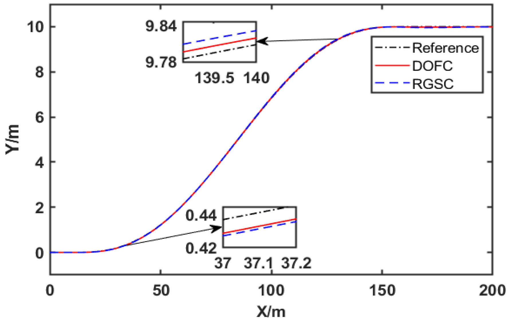
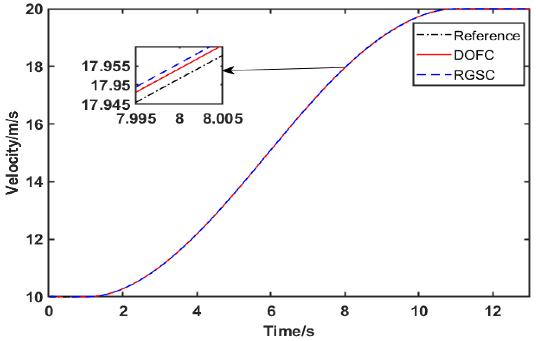
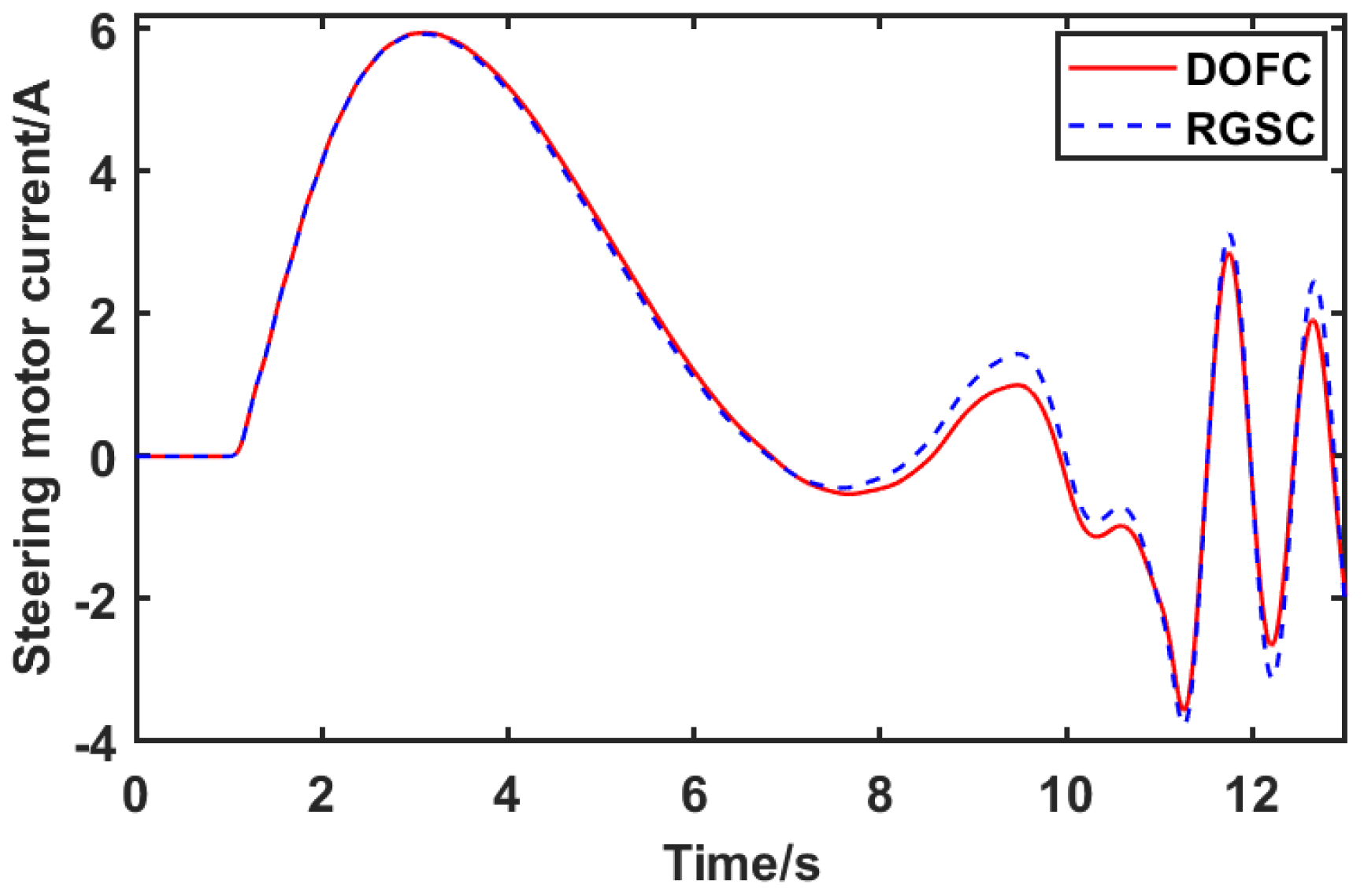
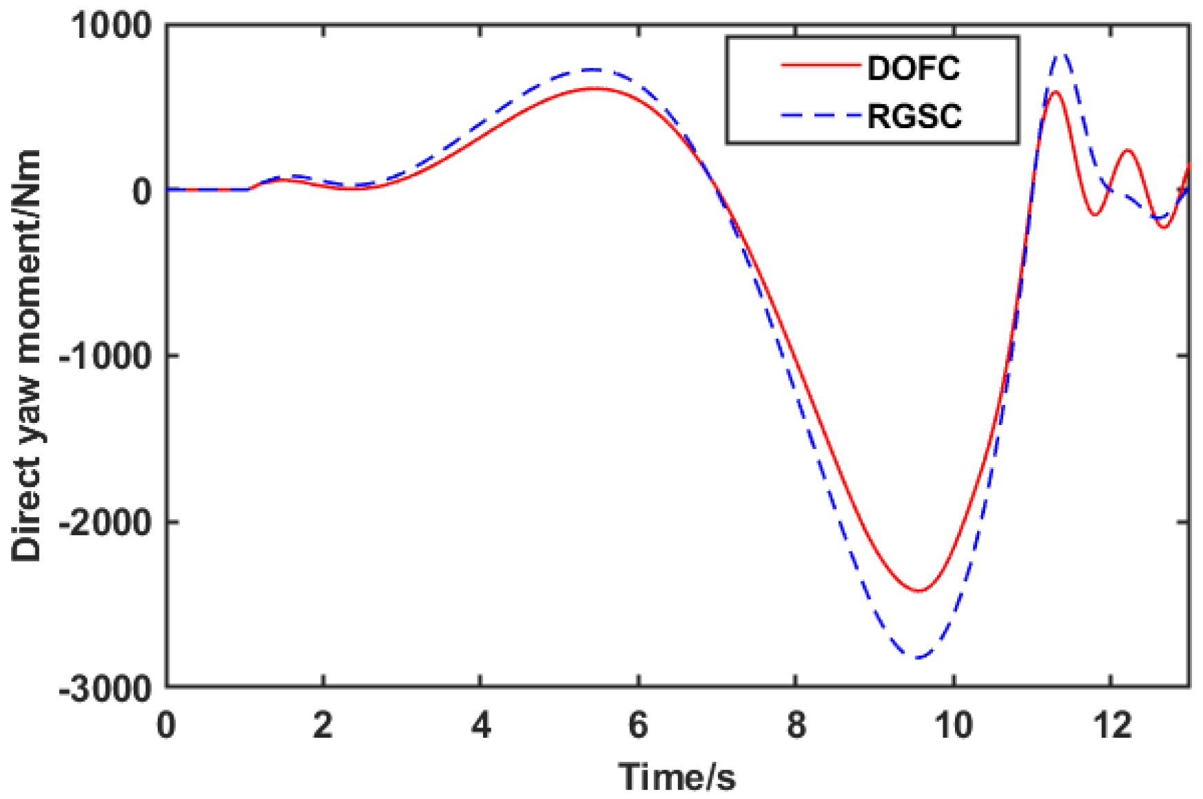
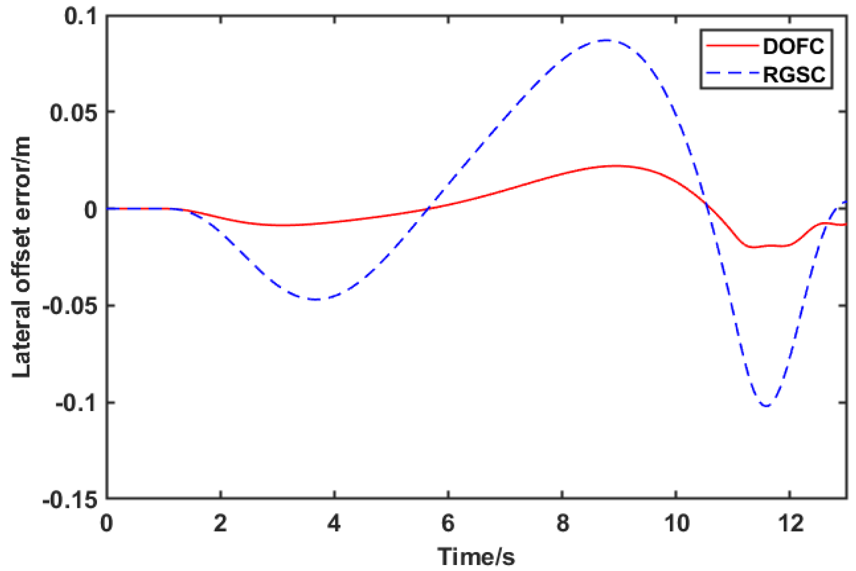
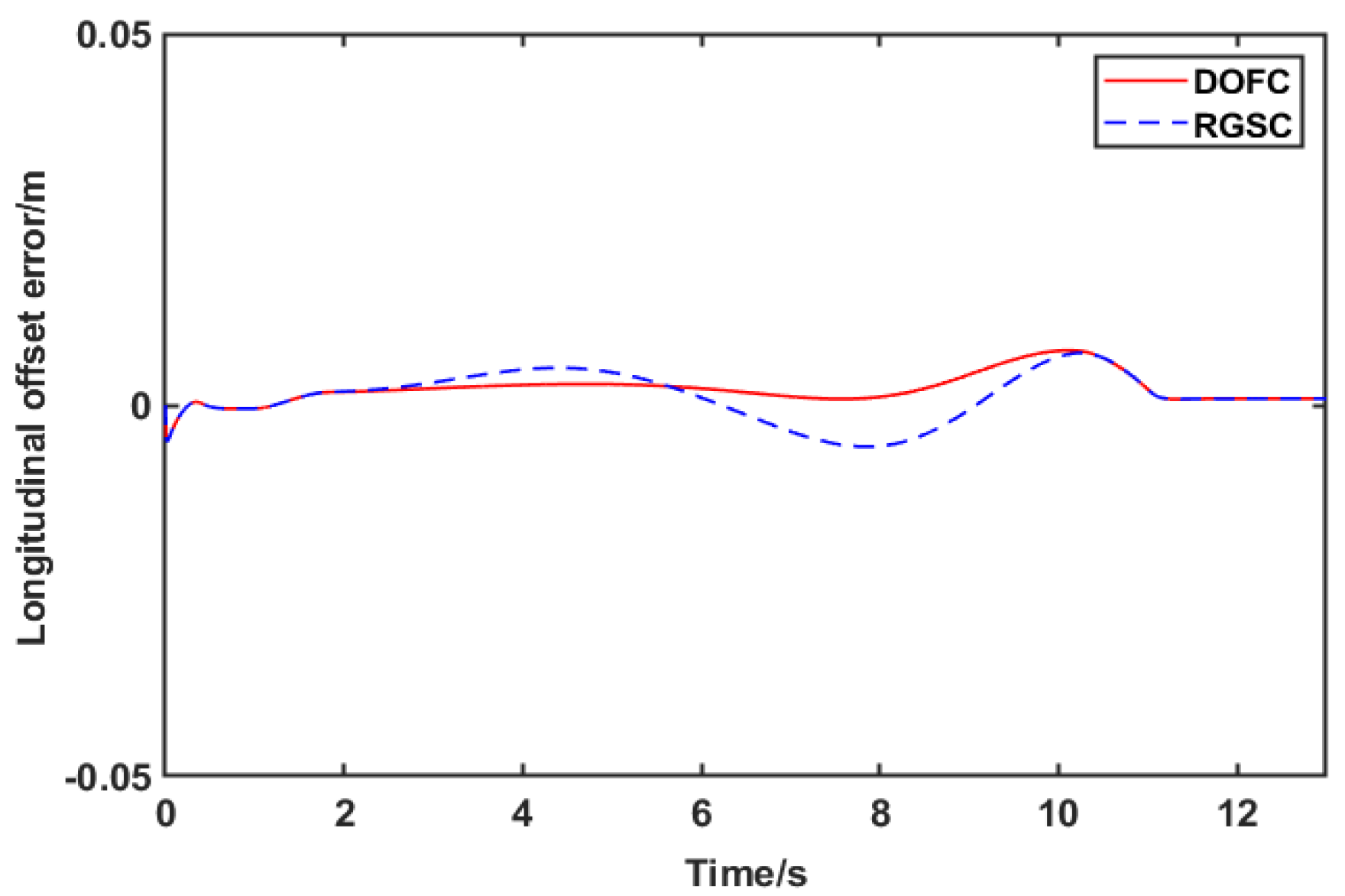
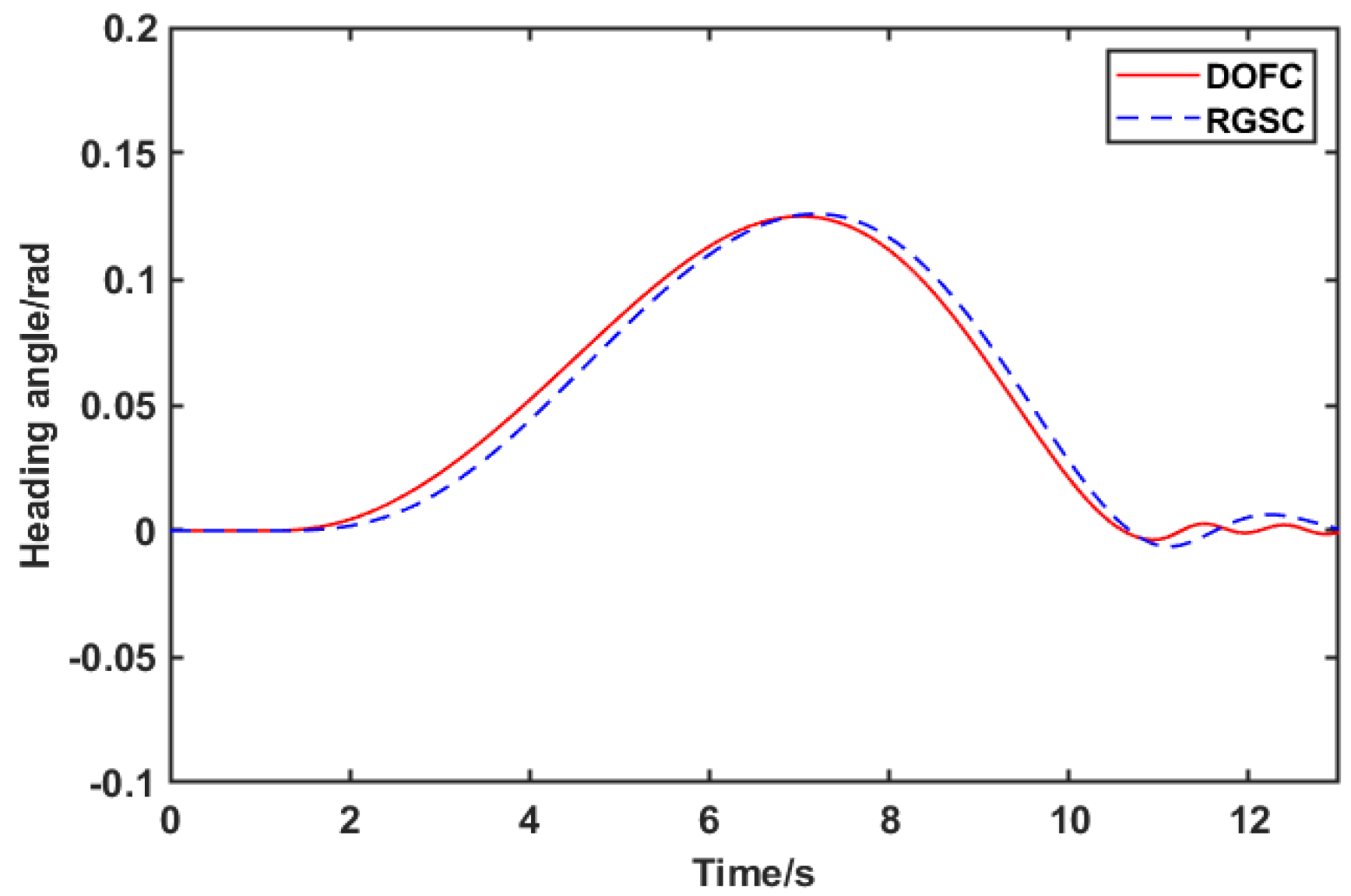
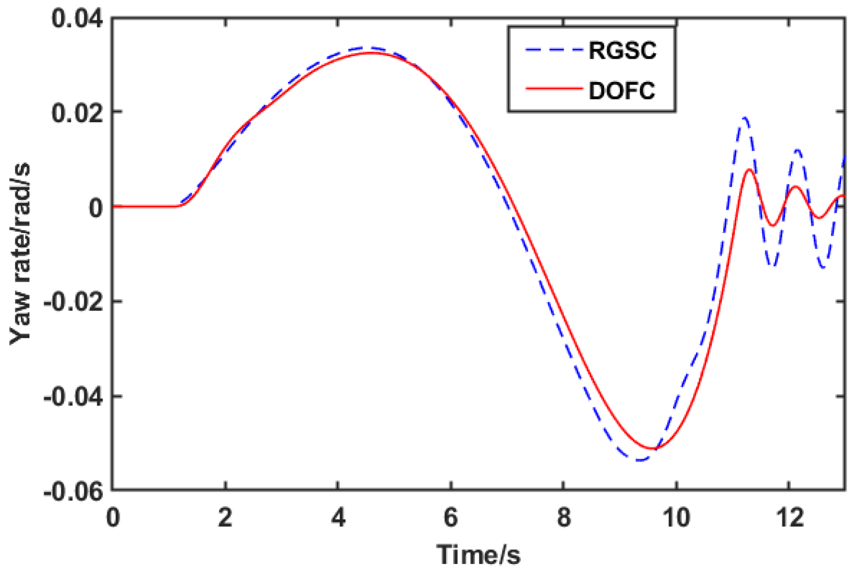
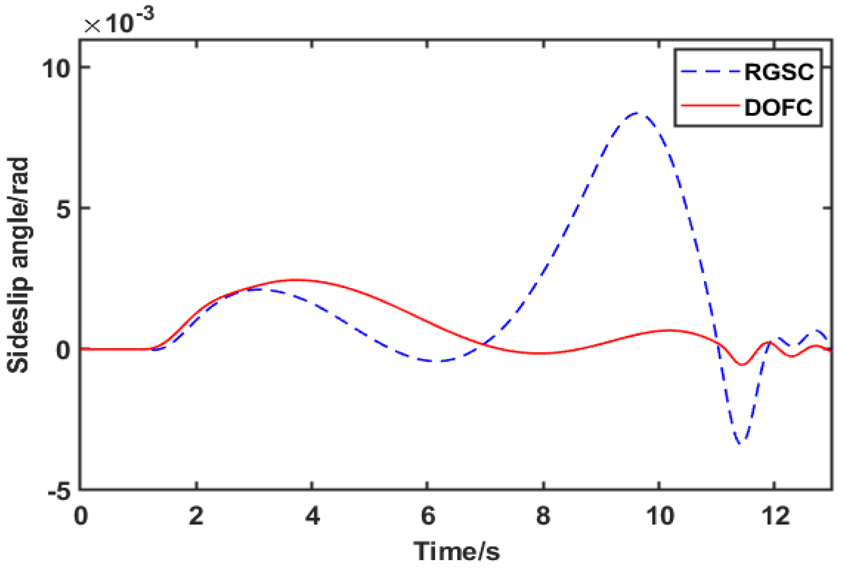
• A trajectory tracking control method with integrated AFS and DYC is proposed for the steer-by-wire FWIA EV, involving the dynamic of steer-by-wire, which is more closely related to the control actuation of the steer-by-wire FWIA EV in reality. Compared with the robust gain-scheduling control (RGSC) strategy not considering the dynamic of the steer-by-wire system, the proposed control strategy can guarantee higher tracking accuracy and better comfort.
• In the proposed integrated control framework, a polyhedral LPV model with eight vertices is established for all the states of the steer-by-wire FWIA EV by considering the time-varying longitudinal velocity and selecting $v_x$, $\frac{1}{v_x}$ and $\frac{1}{v_x^2}$ as scheduling parameters.
• A robust $H_{\infty }$ dynamic output feedback controller without using the vehicle sideslip angle is designed by solving the linear matrix inequalities integrating robust stability, $H_{\infty }$ performance, and actuator constraint, which meets the stability and maneuverability, tracking accuracy, and driving safety requirements in the trajectory tracking process.

The rest of this paper is organized as follows. Section 2 presents the system modeling and problem statement. Section 3 presents a design for a robust dynamic output feedback control using $H_{\infty }$ control theory, linear matrix inequality (LMI), and gain-scheduling method. Section 4 shows the verification results of the effectiveness and advantage of the proposed strategy by comparison with other strategies under the simulation in Carsim-MATLAB/Simulink. Section 5 gives the conclusion.

2. System Modeling and Problem Statement

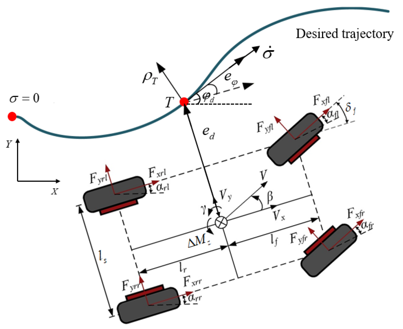
2.1. System Modeling Considering Dynamic Characteristics of Steer-by-Wire

Figure 1 shows the trajectory tracking process of the FWIA EV, where $e_d$ is the lateral deviation, which is the distance between the center of gravity (CG) of the FWIA EV and the nearest point T on the desired trajectory $\sigma$. $e_{\phi }$ is the yaw angle error between the desired yaw angle ${\phi }_d$ and the actual yaw angle $\phi$, which can be expressed as $e_{\phi }={\phi }_d-\phi$.

Consequently, the trajectory tracking error model of the FWIA EV is described as follows [8].

$$\left\{\begin{array}{c}{\dot{e}}_d=v_x{e}_{\phi }+v_x\beta +d_1\hfill \\ {\dot{e}}_{\phi }=\gamma +d_2\hfill \end{array}\right.$$

(1)

where $\beta$ is the sideslip angle. $d_1$ represents the modeling error and external disturbance. $\gamma$ is the yaw rate. $d_2=-{\rho }_T\left(\sigma \right)v_x$, ${\rho }_T\left(\sigma \right)$ is the curvature of the desired trajectory $\sigma$ at point T, $v_x$ is the longitudinal velocity.

Without considering pitch and roll motion, the FWIA EV yaw dynamics model is shown as follows:

$$\left\{\begin{array}{c}\dot{\beta }=\frac{1}{m{v}_x}\left(F_{yf}+F_{yr}\right)+d_3\hfill \\ \dot{\gamma }=\frac{1}{I_z}\left(l_f{F}_{yf}-l_r{F}_{yr}\right)+\frac{1}{I_z}\Delta M_z+d_4\hfill \end{array}\right.$$

(2)

where $F_{yf}$ and $F_{yr}$ are the lateral forces of the front and rear tire, respectively. m is the FWIA EV mass. $I_z$ is the moment of inertia. $l_f$ and $l_r$ are distances from the center of mass of the FWIA EV to the front and rear axes, respectively. $\Delta M_z$ is the direct yaw moment. $d_3$ and $d_4$ denote external disturbances describing unmodeled dynamics and nonlinear terms.

The direct yaw moment $\Delta M_z$ is generated by the difference in longitudinal tire forces between the left and right wheels, expressed as:

$$\Delta M_z={\displaystyle \sum _{i=1}^4}{(-1)}^i{F}_{xi}\frac{l_s}{2}$$

(3)

where $l_s$ denotes the width of the wheel pitch. $F_{xi}$ represents the longitudinal force of the ith tire, controlled by the hub motor.

The wheel dynamics of the FWIA EV can be expressed as

$$I_w{\dot{w}}_i=T_i-F_{xi}{R}_t$$

(4)

where $I_w$ is the wheel’s moment of inertia. $w_i$ is the rotational speed of the ith tire. $T_i$ is the torque of the ith hub motor. $R_t$ denotes the rolling radius of the tire.

The front and rear tire lateral forces $F_{yf}$ and $F_{yr}$ generated by the friction between the tire and the road surface can be described as

$$F_{yf}=\mu C_f{\alpha }_f,F_{yr}=\mu C_r{\alpha }_r$$

(5)

where $\mu$ is the road adhesion coefficient of the front and rear wheels. $C_f$ and $C_r$ are the steering stiffness of the front and rear wheels, respectively. ${\alpha }_f$ and ${\alpha }_r$ are sideslip angles at the front and rear axles, respectively.

According to physical concepts of the slip angles, ${\alpha }_f$ and ${\alpha }_r$ can be expressed as

$${\alpha }_f=\beta +\frac{l_f}{v_x}\gamma -{\delta }_f,{\alpha }_r=\beta -\frac{l_r}{v_x}\gamma$$

(6)

where ${\delta }_f$ is the front-wheel steering angle.

The dynamic of the FWIA EV steering-by-wire system can be written as [27]

$$\begin{array}{c}{\ddot{\delta }}_f=-\frac{\mu C_f\left(l_p+l_m\right)}{J_w}\beta -\frac{\mu C_f{l}_f\left(l_p+l_m\right)}{J_w{v}_x}\gamma +\frac{\mu C_f\left(l_p+l_m\right)}{J_w}{\delta }_f-\frac{b_w}{J_w}{\dot{\delta }}_f+\frac{{\eta }_m{r}_s{k}_m}{J_w}{i}_m+d_5\hfill \end{array}$$

(7)

where $l_p$ and $l_m$ are the aerodynamic trajectory (the distance between the action point of the resultant lateral force and the tire center) and the mechanical trajectory (the distance between the tire center and the steering axis), respectively. $J_w$ is the moment of inertia of the steering system. $b_w$ is the viscous damping. ${\eta }_m$ is the motor efficiency. $r_s$ is the steering ratio. $k_m$ is the motor constant. $i_m$ is the motor current. $d_5$ is the modeling error.

2.2. Polytopic Model Establishment for System Uncertainty

Considering the uncertainties of road adhesion coefficient $\mu \in [{\mu }_{min},{\mu }_{max}]$ and the steering stiffness of the front and rear wheels $C_f\in [C_{fmin},C_{fmax}]$, $C_r\in [C_{rmin},C_{rmax}]$ due to various possible road conditions, and the perturbations of the vehicle mass $m\in [m_{min},m_{max}]$ and yaw inertia $I_z\in [I_{zmin},I_{zmax}]$ due to payload variation, these parameters can be described as follows:

$$\left\{\begin{array}{c}\mu ={\mu }_n+\Delta \mu N_1\left(t\right)\hfill \\ C_f=C_{fn}+\Delta C_f{N}_2\left(t\right)\hfill \\ C_r=C_{rn}+\Delta C_r{N}_3\left(t\right)\hfill \\ \frac{1}{m}=\frac{1}{m_n}+\frac{1}{\Delta m}{N}_4\left(t\right)\hfill \\ \frac{1}{I_z}=\frac{1}{I_{zn}}+\frac{1}{\Delta I_z}{N}_5\left(t\right)\hfill \end{array}\right.$$

(8)

where

$$\begin{array}{c}{\mu }_n=\frac{1}{2}({\mu }_{max}+{\mu }_{min}),\Delta \mu =\frac{1}{2}({\mu }_{max}-{\mu }_{min}),\hfill \\ C_{fn}=\frac{1}{2}(C_{fmax}+C_{fmin}),\Delta C_f=\frac{1}{2}(C_{fmax}-C_{fmin}),\hfill \\ C_{rn}=\frac{1}{2}(C_{rmax}+C_{rmin}),\Delta C_r=\frac{1}{2}(C_{rmax}-C_{rmin}),\hfill \\ m_n=2m_{min}{m}_{max}/(m_{min}+m_{max}),\Delta m=2m_{min}{m}_{max}/(m_{max}-m_{min}),\hfill \\ I_{zn}=2I_{zmin}{I}_{zmax}/(I_{zmin}+I_{zmax}),\Delta I_z=2I_{zmin}{I}_{zmax}/(I_{zmax}-I_{zmin}).\hfill \end{array}$$

and $N_i\left(t\right)$ is a time-varying uncertain parameter with $|N_i\left(t\right)|\le 1$, $i=1,2,\cdots ,5$.

Moreover, the longitudinal velocity $v_x$ varies in the actual trajectory tracking process rather than the constant $v_x$ in conventional lateral control studies. Consequently, this paper regards vehicle longitudinal velocity $v_x$ as a time-varying parameter and defines a time-varying parameter vector $\rho ={[{\rho }_1,{\rho }_2,{\rho }_3]}^T$ by using $v_x$, $\frac{1}{v_x}$ and $\frac{1}{v_x^2}$ with

$${\rho }_1=v_x\in \left[{\underline{v}}_x,{\overline{v}}_x\right],{\rho }_2=\frac{1}{v_x}\in \left[\frac{1}{{\overline{v}}_x},\frac{1}{{\underline{v}}_x}\right],{\rho }_3=\frac{1}{v_x^2}\in \left[\frac{1}{{\overline{v}}_x^2},\frac{1}{{\underline{v}}_x^2}\right]$$

(9)

The FWIA EV is an over-actuated system, the direct yaw moment can be generated by the controlled distribution of the four in-wheel motors, and the control design is usually divided into the trajectory tracking control layer and drive torque distribution layer. In this paper, we focus on the controller design of the FWIA EV trajectory tracking control layer.

Therefore, based on the description on (8) of the system uncertainties and the definition (9) of the time-varying parameters, the trajectory tracking control-oriented dynamic model of the FWIA EV with the steer-by-wire device (1)–(7) can be rewritten as follows.

$$\begin{array}{c}\dot{x}\left(t\right)=A\left(\rho \right)x\left(t\right)+Bu\left(t\right)+B_{d}d\left(t\right)\hfill \\ =\left(A_n\left(\rho \right)+\Delta A\left(\rho \right)\right)x\left(t\right)+\left(B_n+\Delta B\right)u\left(t\right)+\overline{d}\left(t\right)\hfill \end{array}$$

(10)

where $x={\left[e_d,e_{\phi },\beta ,\gamma ,{\delta }_f,{\dot{\delta }}_f\right]}^T$, $u={\left[\Delta M_z,i_m\right]}^T$, and $d\left(t\right)={[d_1,d_2,d_3,d_4,d_5]}^T$ are state variable, control input, and disturbance, respectively. $A\left(\rho \right)$ is system-parameter-dependent matrix, B and $B_d$ are control input and disturbance input matrices, respectively. $A_n\left(\rho \right)$, $B_n$ and $\Delta A\left(\rho \right)$, $\Delta B$ denote the nominal and uncertain parts, respectively.

$A_n\left(\rho \right),B_n,B_d$ are described as:

$A_n\left(\rho \right)=\left[\begin{array}{c}\begin{array}{cccccc}0& {\rho }_1& {\rho }_1& 0& 0& 0\\ 0& 0& 0& 1& 0& 0\\ 0& 0& \frac{c_f+c_r}{m_n}{\rho }_2& \frac{c_f{l}_f-c_r{l}_r}{m_n}{\rho }_3-1& \frac{-c_f}{m_n}{\rho }_2& 0\\ 0& 0& \frac{c_f{l}_f-c_r{l}_r}{I_{zn}}& \frac{c_f{l}_f^2+c_r{l}_r^2}{I_{zn}}{\rho }_2& \frac{-c_f{l}_f}{I_{zn}}& 0\\ 0& 0& 0& 0& 0& 1\\ 0& 0& \frac{-c_f(l_p+l_m)}{J_w}& \frac{-c_f{l}_f(l_p+l_m)}{J_w}{\rho }_2& \frac{c_f(l_p+l_m)}{J_w}& \frac{-b_w}{J_w}\end{array}\end{array}\right]$, $B_n=\left[\begin{array}{cc}0& 0\\ 0& 0\\ 0& 0\\ \frac{1}{I_{zn}}& 0\\ 0& 0\\ 0& \frac{{\eta }_m{r}_s{k}_m}{J_w}\end{array}\right]$, $B_d={\left[\begin{array}{cccccc}1& 0& 0& 0& 0& 0\\ 0& 1& 0& 0& 0& 0\\ 0& 0& 1& 0& 0& 0\\ 0& 0& 0& 1& 0& 0\\ 0& 0& 0& 0& 0& 1\end{array}\right]}^T$,

$c_f={\mu }_n{C}_{fn}$, $c_r={\mu }_n{C}_{rn}$.

The matrices $\Delta A\left(\rho \right)$ and $\Delta B$ only describe the uncertain parts satisfying the condition:

$$\left[\begin{array}{cc}\Delta A\left(\rho \right)& \Delta B\end{array}\right]=H\Lambda \left[\begin{array}{cc}{L}_1\left(\rho \right)& L_2\end{array}\right]$$

(11)

with $\Lambda =\mathrm{diag}\{N_1,N_1,N_1\}$, $\left|N_1\right|\le 1$,

$H={\left[\begin{array}{cccccc}0& 0& 1& 0& 0& 0\\ 0& 0& 0& 1& 0& 0\\ 0& 0& 0& 0& 0& 1\end{array}\right]}^T$, $L_1\left(\rho \right)=\left[\begin{array}{c}\begin{array}{cccccc}0& 0& ({\varphi }_1+{\varphi }_2){\rho }_2& ({\varphi }_1{l}_f-{\varphi }_2{l}_r){\rho }_3& -{\varphi }_1{\rho }_2& 0\\ 0& 0& {\varphi }_3{l}_f-{\varphi }_4{l}_r& ({\varphi }_3{l}_f^2+{\varphi }_4{l}_r^2){\rho }_2& -{\varphi }_3{l}_f& 0\\ 0& 0& \frac{-\Delta c_f(l_p+l_m)}{J_w}& \frac{-\Delta c_f{l}_f(l_p+l_m){\rho }_2}{J_w}& \frac{\Delta c_f(l_p+l_m)}{J_w}& 0\end{array}\end{array}\right]$, $L_2=\left[\begin{array}{cc}0& 0\\ \frac{1}{\Delta I_z}& 0\\ 0& 0\end{array}\right]$,

$\Delta c_f={\mu }_n\Delta C_f+\Delta \mu C_{fn}+\Delta \mu \Delta C_f$, $\Delta c_r={\mu }_n\Delta C_r+\Delta \mu C_{rn}+\Delta \mu \Delta C_r$, ${\varphi }_1=\frac{c_f+\Delta c_f}{\Delta m}+\frac{\Delta c_f}{m_n}$, ${\varphi }_2=\frac{c_r+\Delta c_r}{\Delta m}+\frac{\Delta c_r}{m_n}$, ${\varphi }_3=\frac{c_f+\Delta c_f}{\Delta I_z}+\frac{\Delta c_f}{I_{zn}}$, ${\varphi }_4=\frac{c_r+\Delta c_r}{\Delta I_z}+\frac{\Delta c_r}{I_{zn}}$. And the remaining parts of the uncertainties are combined into the disturbance term $B_{d}d\left(t\right)$ to form the lumped disturbance $\overline{d}\left(t\right)$.

Furthermore, for reducing the computational complexity and design conservativeness, the following polytopic form of the system state-space expression is established as

$$\begin{array}{c}\dot{x}\left(t\right)={\displaystyle \sum _{i=1}^8}{\alpha }_i(\rho ,t)[(A_{ni}+\Delta A_i)x\left(t\right)+\left(B_{ni}+\Delta B_i\right)u\left(t\right)+\overline{d}\left(t\right)]\hfill \\ ={\displaystyle \sum _{i=1}^8}{\alpha }_i(\rho ,t)[(A_{ni}+H\Lambda L_{1i})x\left(t\right)+\left(B_{ni}+H\Lambda L_{2i}\right)u\left(t\right)+\overline{d}\left(t\right)]\hfill \end{array}$$

(12)

where ${\alpha }_i(\rho ,t)$ is barycentric coordinate, defining as

$$\left\{\begin{array}{c}{\alpha }_1(\rho ,t)= |{\rho }_1-{\overline{\rho }}_1\left|\right|{\rho }_2-{\overline{\rho }}_2\left|\right|{\rho }_3-{\overline{\rho }}_3|/\Delta \rho \hfill \\ {\alpha }_2(\rho ,t)= |{\rho }_1-{\underline{\rho }}_1\left|\right|{\rho }_2-{\overline{\rho }}_2\left|\right|{\rho }_3-{\overline{\rho }}_3|/\Delta \rho \hfill \\ {\alpha }_3(\rho ,t)= |{\rho }_1-{\overline{\rho }}_1\left|\right|{\rho }_2-{\underline{\rho }}_2\left|\right|{\rho }_3-{\overline{\rho }}_3|/\Delta \rho \hfill \\ {\alpha }_4(\rho ,t)= |{\rho }_1-{\overline{\rho }}_1|\parallel {\rho }_2-{\overline{\rho }}_2\left|\right|{\rho }_3-{\underline{\rho }}_3|/\Delta \rho \hfill \\ {\alpha }_5(\rho ,t)= |{\rho }_1-{\underline{\rho }}_1\left|\right|{\rho }_2-{\underline{\rho }}_2\left|\right|{\rho }_3-{\overline{\rho }}_3|/\Delta \rho \hfill \\ {\alpha }_6(\rho ,t)= |{\rho }_1-{\underline{\rho }}_1\left|\right|{\rho }_2-{\overline{\rho }}_2\left|\right|{\rho }_3-{\underline{\rho }}_3|/\Delta \rho \hfill \\ {\alpha }_7(\rho ,t)= |{\rho }_1-{\overline{\rho }}_1\left|\right|{\rho }_2-{\underline{\rho }}_2\left|\right|{\rho }_3-{\underline{\rho }}_3|/\Delta \rho \hfill \\ {\alpha }_8(\rho ,t)= |{\rho }_1-{\underline{\rho }}_1\left|\right|{\rho }_2-{\underline{\rho }}_2\left|\right|{\rho }_3-{\underline{\rho }}_3|/\Delta \rho \hfill \end{array}\right.$$

(13)

with $\Delta \rho =|{\overline{\rho }}_1-{\underline{\rho }}_1\left|\right|{\overline{\rho }}_2-{\underline{\rho }}_2\left|\right|{\overline{\rho }}_3-{\underline{\rho }}_3|$, ${\displaystyle \sum _{i=1}^8}{\alpha }_i(\rho ,t)=1.$

$A_{ni},B_{ni},L_{1i},L_{2i}$ are corresponding vertices of system matrices described as

$A_{n1}=A_n({\overline{\rho }}_1,{\overline{\rho }}_2,{\overline{\rho }}_3)$, $A_{n2}=A_n({\underline{\rho }}_1,{\overline{\rho }}_2,{\overline{\rho }}_3)$, $A_{n3}=A_n({\overline{\rho }}_1,{\underline{\rho }}_2,{\overline{\rho }}_3)$, $A_{n4}=A_n({\overline{\rho }}_1,{\overline{\rho }}_2,{\underline{\rho }}_3)$,

$A_{n5}=A_n({\underline{\rho }}_1,{\underline{\rho }}_2,{\overline{\rho }}_3)$, $A_{n6}=A_n({\underline{\rho }}_1,{\overline{\rho }}_2,{\underline{\rho }}_3)$, $A_{n7}=A_n({\overline{\rho }}_1,{\underline{\rho }}_2,{\underline{\rho }}_3)$, $A_{n8}=A_n({\underline{\rho }}_1,{\underline{\rho }}_2,{\underline{\rho }}_3)$, $B_{ni}=B_n$,

$L_{11}=L_1({\overline{\rho }}_1,{\overline{\rho }}_2,{\overline{\rho }}_3)$, $L_{12}=L_1({\underline{\rho }}_1,{\overline{\rho }}_2,{\overline{\rho }}_3)$, $L_{13}=L_1({\overline{\rho }}_1,{\underline{\rho }}_2,{\overline{\rho }}_3)$, $L_{14}=L_1({\overline{\rho }}_1,{\overline{\rho }}_2,{\underline{\rho }}_3)$,

$L_{15}=L_1({\underline{\rho }}_1,{\underline{\rho }}_2,{\overline{\rho }}_3)$, $L_{16}=L_1({\underline{\rho }}_1,{\overline{\rho }}_2,{\underline{\rho }}_3)$, $L_{17}=L_1({\overline{\rho }}_1,{\underline{\rho }}_2,{\underline{\rho }}_3)$, $L_{18}=L_1({\underline{\rho }}_1,{\underline{\rho }}_2,{\underline{\rho }}_3)$, $L_{2i}=L_2$.

2.3. Control Problem Formulation

For the state feedback controller design of the trajectory tracking control layer of the FWIA EVs, all states of $x={\left[e_d,e_{\phi },\beta ,\gamma ,{\delta }_f,{\dot{\delta }}_f\right]}^{\mathrm{T}}$ need to be measured with high accuracy. $e_d$, $e_{\phi }$ can be measured using inexpensive equipment. The yaw rate $\gamma$ can be measured by an onboard sensor or can be synthesized by an accelerometer. However, $\beta$ is often difficult to measure with inexpensive sensors. Therefore, the output feedback-based control scheme is apt to apply to FWIA EVs.

For this reason, this study only takes the states $e_d$, $e_{\phi }$, $\gamma$, ${\delta }_f$, and ${\dot{\delta }}_f$ as the measurement output y. While considering the improvement of trajectory tracking performance, all states are regarded as the evaluation output z. As a result, a trajectory tracking control-oriented model for the steer-by wire FWIA EV can be rewritten as

$$\left\{\begin{array}{c}\dot{x}\left(t\right)={\displaystyle \sum _{i=1}^8}{\alpha }_i(\rho ,t)[(A_{ni}+\Delta A_i)x\left(t\right)+(B_{ni}+\Delta B_i)u\left(t\right)+\overline{d}\left(t\right)]\hfill \\ y\left(t\right)=C_{1}x\left(t\right)\hfill \\ z\left(t\right)=C_{2}x\left(t\right)\hfill \end{array}\right.$$

(14)

where $C_1=\left[\begin{array}{cccccc}1\hfill & 0\hfill & 0\hfill & 0\hfill & 0\hfill & 0\hfill \\ 0\hfill & 1\hfill & 0\hfill & 0\hfill & 0\hfill & 0\hfill \\ 0\hfill & 0\hfill & 0\hfill & 1\hfill & 0\hfill & 0\hfill \\ 0\hfill & 0\hfill & 0\hfill & 0\hfill & 1\hfill & 0\hfill \\ 0\hfill & 0\hfill & 0\hfill & 0\hfill & 0\hfill & 1\hfill \end{array}\right]$, $C_2=I_{6\times 6}$.

The above state space Equation (14) is the FWIA EV’s trajectory tracking control-oriented dynamic model. In the following sections, we focus on the controller design of the FWIA EV trajectory tracking control layer, and the torque distribution is simplified in this paper using a rule-based average distribution method [11].

The control objective is to design a robust $H_{\infty }$ dynamic output feedback controller such that the resulting closed-loop system is robustly stable in the presence of parameter uncertainty and external disturbance and has the $H_{\infty }$ disturbance attenuation properties:

$${\int }_0^t{z}^T\left(t\right)z\left(t\right)\mathrm{d}t\le {\varpi }^2{\int }_0^t{\overline{d}}^T\left(t\right)\overline{d}\left(t\right)\mathrm{d}t$$

(15)

where $\varpi$ is the specified attenuation level.

In addition, from the perspective of safety and mechanical structure, the following constraints should also be satisfied:

$$\left|u_s\left(t\right)\right|\le u_{maxs},s=1,2$$

(16)

where $u_{maxs}$ is the maximum value of $\left|u_s\left(t\right)\right|$, which should be selected according to the road conditions and the maximum torque of the motor.

3. Robust ${\mathbf{H}}_{\infty }$ Output Feedback Trajectory Tracking Control

In order to improve the trajectory tracking performance of the FWIA EV, a robust $H_{\infty }$ dynamic output feedback controller is designed as follows:

$$\left\{\begin{array}{c}{\dot{x}}_c\left(t\right)={\displaystyle \sum _{i=1}^8}{\displaystyle \sum _{j=1}^8}{\alpha }_i(\rho ,t){\alpha }_j(\rho ,t)A_{cij}{x}_c\left(t\right)+{\displaystyle \sum _{j=1}^8}{\alpha }_j(\rho ,t)B_{cj}y\left(t\right)\hfill \\ u={\displaystyle \sum _{j=1}^8}{\alpha }_j(\rho ,t)C_{cj}{x}_c\left(t\right)+D_{c}y\left(t\right)\hfill \end{array}\right.$$

(17)

where $x_c\left(t\right)\in R^6$ is the controller state, and $A_{cij}$, $B_{cj}$, $C_{cj},i,j=1,2,\cdots ,8$ and $D_c$ are the control parameter matrices with the corresponding dimension.

Therefore, the state equation of the resulting closed-loop system can be rewritten as

$$\left\{\begin{array}{c}\dot{\overline{x}}\left(t\right)={\displaystyle \sum _{i=1}^8}{\displaystyle \sum _{j=1}^8}{\alpha }_i(\rho ,t){\alpha }_j(\rho ,t)\left(\left({\overline{A}}_{ij}+\overline{H}\Lambda {\overline{L}}_{ij}\right)\overline{x}\left(t\right)+\overline{B}\overline{d}\left(t\right)\right)\hfill \\ z=\overline{C}\overline{x}\hfill \end{array}\right.$$

(18)

where  $\overline{x}=\left[\begin{array}{c}x\hfill \\ x_c\hfill \end{array}\right],\overline{B}=\left[\begin{array}{c}{I}_{6\times 6}\hfill \\ 0_{2\times 6}\hfill \end{array}\right],\overline{H}=\left[\begin{array}{c}H\\ 0_{2\times 3}\end{array}\right],{\overline{A}}_{ij}=\left[\begin{array}{cc}{A}_{ni}+B_{ni}{D}_c{C}_1& B_{ni}{C}_{cj}\\ B_{cj}{C}_1& A_{cij}\end{array}\right]$,

${\overline{L}}_{ij}=\left[\begin{array}{cc}{L}_{1i}+L_{2i}{D}_c{C}_1\hfill & L_{2i}{C}_{cj}\hfill \end{array}\right],\overline{C}=\left[\begin{array}{cc}{C}_2\hfill & 0_{6\times 2}\hfill \end{array}\right]$.

The following lemma is needed in the subsequent proof of results.

Lemma 1

([11]). Given matrices Y, H, and L of appropriate dimensions, where $Y=Y^T$ then

$$Y+H\Lambda L+L^T{\Lambda }^T{H}^T<0$$

(19)

holds for all time-varying matrices Λ satisfying ${\Lambda }^T\Lambda \le I$, if and only if there is a constant $\epsilon >0$ such that

$$\left[\begin{array}{ccc}Y& \epsilon H& L^T\\ *& -\epsilon I& 0\\ *& *& -\epsilon I\end{array}\right]<0$$

(20)

Theorem 1.

Given the positive constants ϖ and ϑ, if there exist positive scalars ${\epsilon }_{ij},{\epsilon }_{ji}$ and a symmetric positive definite matrix P such that the following matrix inequalities hold, then the closed-loop system (18) is asymptotically stable when $\overline{d}\left(t\right)=0$ and satisfies the $H_{\infty }$ performance index (15) for all $\overline{d}\left(t\right)$.

$$\begin{array}{ccc}& & {\overline{{\rm Y}}}_{1ij}+{\overline{{\rm Y}}}_{1ji}<0,1\le i\le j\le 8\hfill \end{array}$$

(21)

$$\begin{array}{ccc}& & {\overline{{\rm Y}}}_{2sj}<0,s=1,2,j=1,2,\cdots ,8\hfill \end{array}$$

(22)

where matrices ${\overline{{\rm Y}}}_{1ij}$, ${\overline{{\rm Y}}}_{1ji}$, and ${\overline{{\rm Y}}}_{2sj}$ are defined as

${\overline{{\rm Y}}}_{1ij}=\left[\begin{array}{ccccc}{\overline{A}}_{ij}^{T}P+P{\overline{A}}_{ij}& P\overline{B}& {\overline{C}}^T& P\overline{H}& {\overline{L}}_{ij}^T\\ *& -I& 0& 0& 0\\ *& *& -{\varpi }^{2}I& 0& 0\\ *& *& *& -{\epsilon }_{ij}^{-1}I& 0\\ *& *& *& *& -{\epsilon }_{ij}I\end{array}\right]$,  ${\overline{{\rm Y}}}_{2sj}=\left[\begin{array}{cc}-u_{maxs}^{2}P& K_{hj}^{\mathrm{T}}\\ & -{\vartheta }^{-1}I\end{array}\right]$,

${\overline{{\rm Y}}}_{1ji}=\left[\begin{array}{ccccc}{\overline{A}}_{ji}^{T}P+P{\overline{A}}_{ji}& P\overline{B}& {\overline{C}}^T& P\overline{H}& {\overline{L}}_{ji}^T\\ & -I& 0& 0& 0\\ & *& -{\varpi }^{2}I& 0& 0\\ & *& *& -{\epsilon }_{ji}^{-1}I& 0\\ & *& *& *& -{\epsilon }_{ji}I\end{array}\right]$,  $K_{hj}=\left[\begin{array}{cc}{D}_c{C}_1\hfill & C_{cj}\hfill \end{array}\right]$.

Proof. 

For the closed-loop system (18), the Lyapunov function is chosen as

$$V\left(\overline{x}\right)={\overline{x}}^T\left(t\right)P\overline{x}\left(t\right)$$

(23)

then, calculating the time derivative of V and considering $z^T\left(t\right)z\left(t\right)-{\varpi }^2{\overline{d}}^T\left(t\right)\overline{d}\left(t\right)$ with $\varpi >0$, there is the following equality.

$$\begin{array}{c}\dot{V}\left(\overline{x}\right)+z^T\left(t\right)z\left(t\right)-{\varpi }^2{\overline{d}}^T\left(t\right)\overline{d}\left(t\right)\hfill \\ ={\displaystyle \sum _{i=1}^8}{\displaystyle \sum _{j=1}^8}{\alpha }_i(\rho ,t){\alpha }_j(\rho ,t)\left({\overline{x}}^T\left(t\right){\Theta }_{ij}\overline{x}\left(t\right)+2{\overline{x}}^T\left(t\right)P\overline{B}\overline{d}\left(t\right)+z^T\left(t\right)z\left(t\right)-{\varpi }^2{\overline{d}}^T\left(t\right)\overline{d}\left(t\right)\right)\hfill \\ ={\displaystyle \sum _{i=1}^8}{\displaystyle \sum _{j=1}^8}{\alpha }_i(\rho ,t){\alpha }_j(\rho ,t){\left[\begin{array}{c}\overline{x}\left(t\right)\\ \overline{d}\left(t\right)\end{array}\right]}^T{{\rm Y}}_{1ij}\left[\begin{array}{c}\overline{x}\left(t\right)\\ \overline{d}\left(t\right)\end{array}\right]\hfill \end{array}$$

(24)

where ${\Theta }_{ij}={\overline{A}}_{ij}^{T}P+P{\overline{A}}_{ij}+P\overline{H}\Lambda {\overline{L}}_{ij}+{\overline{L}}_{ij}^T\Lambda {\overline{H}}^{T}P$,  ${{\rm Y}}_{1ij}=\left[\begin{array}{cc}{\Theta }_{ij}+{\overline{C}}^T\overline{C}& P\overline{B}\\ {\overline{B}}^{T}P& -{\varpi }^{2}I\end{array}\right]$.

Thus, it can be concluded that if the following inequality holds,

$${\displaystyle \sum _{i=1}^8}{\displaystyle \sum _{j=1}^8}{\alpha }_i(\rho ,t){\alpha }_j(\rho ,t){{\rm Y}}_{1ij}<0$$

(25)

then the closed-loop control system (18) will be robustly asymptotically stable when $\overline{d}\left(t\right)=0$ and can satisfy the $H_{\infty }$ performance index (15) for all $\overline{d}\left(t\right)$.

Furthermore, the inequality (25) can be rewritten as

$${\displaystyle \sum _{i=1}^8}{\alpha }_i^2(\rho ,t){{\rm Y}}_{1ii}+{\displaystyle \sum _{i=1}^7}{\displaystyle \sum _{j=i+1}^8}{\alpha }_i(\rho ,t){\alpha }_j(\rho ,t)\left({{\rm Y}}_{1ij}+{{\rm Y}}_{1ji}\right)<0$$

(26)

Consequently, if the following conditions hold,

$${{\rm Y}}_{1ij}+{{\rm Y}}_{1ji}<0,1\le i\le j\le 8$$

(27)

the controlled system is robustly stable and has $H_{\infty }$ the performance index (15).

By using Schur’s complement lemma to (27), the following inequality follows:

$$\left[\begin{array}{c}\begin{array}{ccc}{\Theta }_{ij}& P\overline{B}& {\overline{C}}^T\\ *& -{\varpi }^{2}I& 0\\ *& *& -I\end{array}\end{array}\right]+\left[\begin{array}{c}\begin{array}{ccc}{\Theta }_{ji}& P\overline{B}& {\overline{C}}^T\\ *& -{\varpi }^{2}I& 0\\ *& *& -I\end{array}\end{array}\right]<0$$

(28)

According to Lemma 1, there is the following inequality:

$$\left[\begin{array}{ccccc}{\overline{A}}_{ij}^{T}P+P{\overline{A}}_{ij}& P\overline{B}& {\overline{C}}^T& {\epsilon }_{ij}P\overline{H}& {\overline{L}}_{ij}^T\\ *& -{\varpi }^{2}I& 0& 0& 0\\ *& *& -I& 0& 0\\ *& *& *& -{\epsilon }_{ij}I& 0\\ *& *& *& *& -{\epsilon }_{ij}I\end{array}\right]+\left[\begin{array}{ccccc}{\overline{A}}_{ji}^{T}P+P{\overline{A}}_{ji}& P\overline{B}& {\overline{C}}^T& {\epsilon }_{ji}P\overline{H}& {\overline{L}}_{ji}^T\\ *& -{\varpi }^{2}I& 0& 0& 0\\ *& *& -I& 0& 0\\ *& *& *& -{\epsilon }_{ji}I& 0\\ *& *& *& *& -{\epsilon }_{ji}I\end{array}\right]<0$$

(29)

The congruence transformation of the inequality (29) is performed using the diagonal matrix $\mathrm{diag}\left\{I,I,I,{({\epsilon }_{ij}+{\epsilon }_{ji})}^{-1}I,I\right\}$. Thus, the inequality (21) holds.

The following proves the inequality (22). The system is asymptotically stable when $\overline{d}\left(t\right)=0$, and the performance index (15) satisfies for all $\overline{d}\left(t\right)$, if

$$\dot{V}\left(t\right)+z^T\left(t\right)z\left(t\right)-{\varpi }^2{\overline{d}}^T\left(t\right)\overline{d}\left(t\right)\le 0,\forall \overline{x}\left(t\right),\overline{d}\left(t\right)$$

(30)

Then, integrating both sides of the inequality (30) from 0 to t, there follows

$$V\left(t\right)\le {\varpi }^2{\int }_0^t{\overline{d}}^T\left(t\right)\overline{d}\left(t\right)\mathrm{d}t+V\left(0\right)={\varpi }^2{\parallel \overline{d}\left(t\right)\parallel }_2^2+V\left(0\right)\le \vartheta ,\forall t\ge 0$$

(31)

where $\vartheta :={\varpi }^2{\overline{d}}_{max}+V\left(0\right)$, ${\overline{d}}_{max}:=max\{\parallel \overline{d}\left(t\right){\parallel }_2^2\},\forall t\ge 0$.

Considering the controller (17) with $K_h:=\left[\begin{array}{cc}{D}_c{C}_1& {\displaystyle \sum _{j=1}^8}{\alpha }_j(\rho ,t)C_{cj}\end{array}\right]$, then $u=K_h\overline{x}\left(t\right)$.

Defining $\tilde{x}=P^{1/2}\overline{x}$ and using ${\tilde{x}}^T\left(t\right)\tilde{x}\left(t\right)={\overline{x}}^T\left(t\right)P\overline{x}\left(t\right)\le \vartheta$, there is

$$\begin{array}{cc}\hfill {\left|u_s\left(t\right)\right|}^2& \le \underset{t\ge 0}{max}{∥{\overline{x}}^T\left(t\right)K_h^T{K}_h\overline{x}\left(t\right)∥}_2^2\hfill \\ \hfill & =\underset{t\ge 0}{max}{∥{\tilde{x}}^T\left(t\right)P^{-1/2}{K}_h^T{K}_h{P}^{-1/2}\tilde{x}\left(t\right)∥}_2^2\hfill \\ \hfill & \le \vartheta {\lambda }_{max}\left(P^{-1/2}{K}_h^T{K}_h{P}^{-1/2}\right),s=1,2\hfill \end{array}$$

(32)

where ${\lambda }_{max}(·)$ represents the largest eigenvalue of the matrix.

Therefore, if $\vartheta P^{-1/2}{K}_h^T{K}_h{P}^{-1/2}<u_{maxs}^{2}I$, the constraint (16) will satisfy. Furthermore, using Schur’s complement and considering ${\displaystyle \sum _{j=1}^8}{\alpha }_j(\rho ,t)=1$, the following inequality holds.

$$\left[\begin{array}{cc}-u_{max s}^{2}P& K_h^T\\ *& -{\vartheta }^{-1}I\end{array}\right]={\displaystyle \sum _{j=1}^8}{\alpha }_j(\rho ,t)\left[\begin{array}{cc}-u_{max s}^{2}P& K_{hj}^T\\ *& -{\vartheta }^{-1}I\end{array}\right]={\displaystyle \sum _{j=1}^8}{\alpha }_j(\rho ,t){\overline{{\rm Y}}}_{2sj}<0$$

(33)

Therefore, the constraint (16) satisfies when (22) holds. This completes the proof. □

Remark 1.

It should be noted that the inequality (22) is a constraint on the gains of the designed controller (17) according to the actuator constraint (16). The parameter ϑ is just an assignment (a large value should be selected) involving the maximum bound value of the lumped disturbance and the system’s initial condition. The exact bound value of $\overline{d}\left(t\right)$ is not required. Meanwhile, it should be pointed out that the inequalities (21) and (22) are only sufficient conditions for the existence of an output feedback controller (17) satisfying the control performance requirements (robustly stable and $H_{\infty }$ performance (15) and actuator constraint (16). The sufficient conditions for solving the control parameter matrices $A_{cij},B_{cj},C_{cj},D_c(i,j=1,2,\cdots ,8)$ are not given.

The following will give a solvable condition for the control parameter matrices $A_{cij}$, $B_{cj}$, $C_{cj}$, and $D_c$ through the mathematical transformation technique.

The non-singular matrix P and its inverse matrix $P^{-1}$ can be partitioned into the following block forms.

$$P=\left[\begin{array}{cc}R& F\\ F^T& W\end{array}\right],P^{-1}=\left[\begin{array}{cc}S& E\\ E^T& V\end{array}\right]$$

(34)

with symmetric positive definite matrices R and S, full-rank matrices E and F, $E{F}^T=I-SR$, and define

$$Q_1=\left[\begin{array}{cc}S& I\\ E^T& 0\end{array}\right],Q_2=\left[\begin{array}{cc}I& R\\ 0& F^T\end{array}\right]$$

(35)

then, there exists the following result.

Theorem 2.

Given the positive constants ϖ and ϑ, if there are symmetric positive definite matrices R and S, positive scalars ${\epsilon }_{ij}$ and ${\epsilon }_{ji}$, and matrices ${\widehat{A}}_{cij}$, ${\widehat{B}}_{cj}$, ${\widehat{C}}_{cj}$, and ${\widehat{D}}_c$, such that the following matrix inequalities hold, the closed-loop system (18) is asymptotically stable when $\overline{d}\left(t\right)=0$ and satisfies the $H_{\infty }$ performance index (15) for all $\overline{d}\left(t\right)$.

$$\begin{array}{ccc}& & {\Xi }_{1ij}+{\Xi }_{1ji}<0,1\le i\le j\le 8\hfill \end{array}$$

(36)

$$\begin{array}{ccc}& & {\Xi }_{2sj}<0,s=1,2,j=1,2,\cdots ,8\hfill \end{array}$$

(37)

where ${\Xi }_{1ij}$, ${\Xi }_{1ji}$, and ${\Xi }_{2sj}$ are defined as

$$\left\{\begin{array}{c}{\Xi }_{1ij}=\left[\begin{array}{cccccc}{G}_{ij}+G_{ij}^T& {\widehat{A}}_{cij}+K_i& I& S{C}_2^T& H& S{L}_{1i}^T+{\widehat{C}}_{cj}^T{L}_{2i}^T\\ *& J_{ij}+J_{ij}^T& R& C_2^T& RH& L_{1i}^T+C_1^T{\widehat{D}}_c^T{L}_{2i}^T\\ *& *& -I& 0& 0& 0\\ *& *& *& -{\varpi }^{2}I& 0& 0\\ *& *& *& *& -{\epsilon }_{ij}^{-1}I& 0\\ *& *& *& *& *& -{\epsilon }_{ij}I\end{array}\right],\hfill \\ {\Xi }_{1ji}=\left[\begin{array}{cccccc}{G}_{ji}+G_{ji}^T& {\widehat{A}}_{cji}+K_i& I& S{C}_2^T& H& S{L}_{1i}^T+{\widehat{C}}_{cj}^T{L}_{2i}^T\\ *& J_{ji}+J_{ji}^T& R& C_2^T& RH& L_{1i}^T+C_1^T{\widehat{D}}_c^T{L}_{2i}^T\\ *& *& -I& 0& 0& 0\\ *& *& *& -{\varpi }^{2}I& 0& 0\\ *& *& *& *& -{\epsilon }_{ji}^{-1}I& 0\\ *& *& *& *& *& -{\epsilon }_{ji}I\end{array}\right],\hfill \\ {\Xi }_{2sj}=\left[\begin{array}{ccc}-u_{maxs}^{2}S& -u_{maxs}^{2}I& {\widehat{C}}_{cj}^T\\ *& -u_{maxs}^{2}R& C_1^T{\widehat{D}}_c^T\\ *& *& -{\vartheta }^{-1}I\end{array}\right].\hfill \end{array}\right.$$

(38)

with $G_{ij}=A_{ni}S+B_{ni}{\widehat{C}}_{cj}$,  $K_i=A_{ni}+B_n{\widehat{D}}_c{C}_1$,  $J_{ij}=R{A}_{ni}+{\widehat{B}}_{cj}{C}_1$

Furthermore, the control parameter matrices $A_{cij},B_{cj},C_{cj},D_c,i,j=1,2,\cdots ,8$ of the controller (17) can be obtained as follows.

$$\left\{\begin{array}{c}{A}_{cij}=F^{-1}\left[{\widehat{A}}_{cij}-R(A_{ni}+B_{ni}{D}_c{C}_1)S\right]E^{-T}-B_{cj}{C}_{1}S{E}^{-T}-F^{-1}R{B}_{ni}{C}_{cj}\hfill \\ B_{cj}=F^{-1}({\widehat{B}}_{cj}-R{B}_{ni}{D}_c)\hfill \\ C_{cj}=({\widehat{C}}_{cj}-D_c{C}_{1}S)E^{-T}\hfill \\ D_c={\widehat{D}}_c\hfill \end{array}\right.$$

(39)

Proof. 

By performing congruence transformations with $\mathrm{diag}\left\{Q_1,I,I,I,I\right\}$ to ${\overline{{\rm Y}}}_{1ij}/{\overline{{\rm Y}}}_{1ji}$ in the inequality (21) and $\mathrm{diag}\left\{Q_1,I\right\}$ to ${\overline{{\rm Y}}}_{2sj}$ in (22), the following equalities hold.

$$\left\{\begin{array}{c}{\Xi }_{1ij}=\left[\begin{array}{ccccc}{Q}_1^T{\overline{A}}_{ij}^{T}P{Q}_1+Q_1^{T}P{\overline{A}}_{ij}{Q}_1& Q_1^{T}P\overline{B}& Q_1^T{\overline{C}}^T& Q_1^{T}P\overline{H}& Q_1^T{\overline{L}}_{ij}^T\\ *& -{\varpi }^{2}I& 0& 0& 0\\ *& *& -I& 0& 0\\ *& *& *& -{\epsilon }_{1ij}^{-1}I& 0\\ *& *& *& *& -{\epsilon }_{1ij}I\end{array}\right],\hfill \\ {\Xi }_{1ji}=\left[\begin{array}{ccccc}{Q}_1^T{\overline{A}}_{ji}^{T}P{Q}_1+Q_1^{T}P{\overline{A}}_{ji}{Q}_1& Q_1^{T}P\overline{B}& Q_1^T{\overline{C}}^T& Q_1^{T}P\overline{H}& Q_1^T{\overline{L}}_{ji}^T\\ *& -{\varpi }^{2}I& 0& 0& 0\\ *& *& -I& 0& 0\\ *& *& *& -{\epsilon }_{1ji}^{-1}I& 0\\ *& *& *& *& -{\epsilon }_{1ji}I\end{array}\right],\hfill \\ {\Xi }_{2sj}=\left[\begin{array}{cc}-u_{maxs}^2{Q}_1^{T}P{Q}_1& Q_1^T{K}_{hj}^T\\ *& {\vartheta }^{-1}I\end{array}\right]\hfill \end{array}\right.$$

(40)

According to the definitions of $Q_1$ and $Q_2$, then $P{Q}_1=Q_2$, there are

$$\left\{\begin{array}{c}{Q}_1^{T}P{\overline{A}}_{ij}{Q}_1=Q_2^T{\overline{A}}_{ij}{Q}_1=\left[\begin{array}{cc}{A}_{ni}S+B_{ni}{\widehat{C}}_{cj}& A_{ni}+B_{ni}{\widehat{D}}_c{C}_1\\ {\widehat{A}}_{cij}& R{A}_{ni}+{\widehat{B}}_{cj}{C}_1\end{array}\right],\hfill \\ Q_1^{T}P\overline{B}=\left[\begin{array}{cc}I& 0\\ R& F\end{array}\right]\left[\begin{array}{c}I\\ 0\end{array}\right]=\left[\begin{array}{c}I\\ R\end{array}\right],\hfill \\ Q_1^T{\overline{C}}^T=\left[\begin{array}{cc}S& E\\ I& 0\end{array}\right]\left[\begin{array}{c}{C}_2^T\\ 0\end{array}\right]=\left[\begin{array}{c}S{C}_2^T\\ C_2^T\end{array}\right],\hfill \\ Q_1^{T}P\overline{H}=\left[\begin{array}{cc}I& 0\\ R& F\end{array}\right]\left[\begin{array}{c}H\\ 0\end{array}\right]=\left[\begin{array}{c}H\\ RH\end{array}\right],\hfill \\ Q_1^T{\overline{L}}_{ij}^T=\left[\begin{array}{cc}S& E\\ I& 0\end{array}\right]\left[\begin{array}{c}{L}_{1i}^T+{\left(L_{2i}{D}_c{C}_1\right)}^T\\ {\left(L_{2i}{C}_{cj}\right)}^T\end{array}\right]=\left[\begin{array}{c}S{L}_{1i}^T+{\widehat{C}}_{cj}^T{L}_{2i}^T\\ L_{1i}^T+C_1^T{\widehat{D}}_c^T{L}_{2i}^T\end{array}\right],\hfill \\ Q_1^{T}P{Q}_1=\left[\begin{array}{cc}S& I\\ RS+F{E}^T& R\end{array}\right]=\left[\begin{array}{cc}R& I\\ I& S\end{array}\right],\hfill \\ K_{hj}{Q}_1=\left[\begin{array}{cc}{D}_c{C}_1& C_{cj}\end{array}\right]\left[\begin{array}{cc}S& I\\ E^T& 0\end{array}\right]=\left[\begin{array}{cc}{\widehat{C}}_{cj}& {\widehat{D}}_c{C}_1\end{array}\right],\hfill \end{array}\right.$$

(41)

where

$$\left\{\begin{array}{c}{\widehat{A}}_{cij}=R\left(A_{ni}+B_{ni}{D}_c{C}_1\right)S+F{B}_{cj}{C}_{1}S+R{B}_{ni}{C}_{cj}{E}^T+F{A}_{cij}{E}^T\hfill \\ {\widehat{B}}_{cj}=R{B}_{ni}{D}_c+F{B}_{cj}\hfill \\ {\widehat{C}}_{cj}=D_c{C}_{1}S+C_{cj}{E}^T\hfill \\ {\widehat{D}}_c=D_c,(i,j=1,2,\cdots ,8)\hfill \end{array}\right.$$

(42)

Substituting (41) into (40) follows (38). Consequently, the inequalities (36) and (37) hold. Moreover, (39) can be obtained through (42). This completes the proof.

Remark 2.

It should be noted that the order of the above designed controller is the same as that of the controlled plant (14). However, the controller’s order can be appropriately reduced under the premise that the control performance is unaffected.

4. Simulation Validation

In this section, the performance of the proposed controller is evaluated through simulation verification. A high-fidelity car model was constructed in CarSim-MATLAB/Simulink based on the actual steer-by-wire FWIA EV experimental data. In the co-simulation platform, the dynamic output feedback controller was designed in MATLAB/Simulink, and the communications of co-simulation between MATLAB/Simulink and CarSim were achieved by a CarSim S-Function connection with interface functions [11]. 

Table 1. Vehicle parameters.

Symbol	Definition	Value
m	Vehicle mass	1830 kg
$I_z$	Vehicle yaw moment of inertia	3234 kg m${}^2$
$J_w$	Moment of inertia in steering system	10.0035 kg m${}^2$
$b_w$	Viscous damping	350.1 Nm s/rad
$k_m$	Motor constant	0.078 Nm/A
$l_p$	Aerodynamic trajectory	0.036 m
$l_m$	Mechanical trajectory	0.024 m
${\eta }_m$	Motor efficiency	0.7
$r_s$	Steering ratio	30
$l_f$	Distance of CG from front axle	1.4 m
$l_r$	Distance of CG from rear axle	1.65 m
$C_f$	Cornering stiffness of front tires	−134.843 kN/rad
$C_r$	Cornering stiffness of rear tires	−124.337 kN/rad
$l_s$	Vehicle tread	1.5 m
R	Tire radius	0.3 m

lists the vehicle parameters.

The accelerated lane-change scene was selected for simulation verification, in which the planning layer gives the reference trajectory, the road surface adhesion coefficient is 0.5, and there is 30% perturbation in the system parameters. To fully illustrate the advantage of considering the dynamic of the steer-by-wire in the control design, we compared the designed dynamic output feedback controller (DOFC) in this paper with the robust gain-scheduling control (RGSC) given in [24]. The design of DOFC considers the dynamic characteristics of the steer-by-wire system. In contrast, the design of RGSC does not consider the dynamic characteristics of the steer-by-wire system. Both controllers adopt the integrated control of AFS and DYC, and the longitudinal control adopts the same double closed-loop PID control. When designing the two controllers, the range of time-varying speed was selected as 5–30 m/s. The simulation results are as follows.

It can be seen from Figure 2 and Figure 3 that both control methods can make the FWIA EV track the reference trajectory with a small tracking error. However, the DOFC controller has a minor overshoot for reference trajectory and reference velocity tracking, higher tracking accuracy, and better tracking effect. The RGSC controller has a larger overshoot for reference trajectory and reference velocity tracking.

It can be seen from Figure 4 that during acceleration and lane change, the steering motor currents of the two controllers both change between −6A and 6A, and the trend of change is the same, but the steering current required by the DOFC controller is slightly less than the steering current required by the RGSC controller. It can be seen from Figure 5 that during the lane-change acceleration process, the direct yaw moments required by the two controllers both vary between −2500 and 600 Nm, and the trend of change is the same, but the direct yaw moment required by the DOFC controller is slightly less than the direct yaw moment required by the RGSC controller. Therefore, it means that when performing the same acceleration and lane change, the control quantity required by the DOFC controller considering the dynamic characteristics of the steer-by-wire system is slightly smaller than that required by the RGSC controller without considering the dynamic characteristics of the steer-by-wire system.

As shown in Figure 6, during the lane-change acceleration process, the lateral offset error of the DOFC controller fluctuates between $-0.04$ and 0.04 m, and the average absolute error value of the lateral offset is 0.01454 m; during the lane-change acceleration process, the lateral offset of the RGSC controller is between −0.10 and 0.09 m, and the average absolute error value of the lateral offset is 0.03685 m. This means that the average absolute error of lateral offset of the DOFC controller is minor, and the tracking effect is better than the RGSC. As shown in Figure 7, during the lane-change acceleration process, the average absolute error of the longitudinal offset of the DOFC controller is 0.00215 m, and the average absolute error of the longitudinal offset of the RGSC controller is 0.00246 m. When performing the same acceleration and changing lanes, the DOFC controller that considers the dynamic characteristics of the steer-by-wire system has a better control effect than the RGSC controller that does not consider the dynamic characteristics of the steer-by-wire system.

As shown in Figure 8 and Figure 9, the two controllers’ heading angle and yaw rate are tiny, ensuring the stability and safety of the FWIA EV during acceleration and lane change. However, when driving from a curve to a straight line in 11 s, the overshoot of the yaw rate of the DOFC controller is slight, and the convergence speed is fast. In contrast, the overshoot of the yaw rate of the RGSC controller is relatively large, and the convergence speed is relatively slow. Therefore, the DOFC controller can give the FWIA EV better ride comfort. As shown in Figure 10, the maximum sideslip angle of the DOFC controller is small, and the maximum sideslip angle of the RGSC controller is relatively large. The maximum sideslip angle of the two controllers is less than 0.009 rad, which will not affect the vehicle’s stability and safety. This means that the comfort of the closed-loop system enforced by the DOFC controller is better than that of the RGSC.

5. Conclusions

This paper investigated the trajectory tracking control issue of the steer-by-wire FWIA EV by integrating AFS and DYC, mainly focusing on considering the dynamic of the steer-by-wire device, time-varying longitudinal velocity, parameter uncertainty, and external disturbances. Based on establishing an LPV model of all the state of the steer-by-wire FWIA EV, this paper proposed a robust $H_{\infty }$ dynamic output feedback control strategy without using the vehicle sideslip angle measure to achieve the stability, safety, maneuverability, and tracking accuracy requirements in the practical application of the FWIA EV. The control parameter matrices of the designed dynamic output feedback controller were obtained by solving the linear matrix inequalities integrating robust stability, $H_{\infty }$ performance, and actuator constraint. Compared with the control strategy without considering the dynamic of the steer-by-wire in [24], the effectiveness and advantages of the proposed control strategy were verified under a CarSim-MATLAB/Simulink simulation environment. The simulation results show that the proposed control strategy can ensure high tracking accuracy and better comfort than the strategy without considering the dynamic of the steer-by-wire system.

In addition, it can be noted that the control parameter matrices are obtained by solving a series of linear matrix inequalities. Now the order of the controller solved is the same as the order of the controlled plant. The higher the order of the controlled plant, the higher the controller’s order, the more difficult it is to solve the inequalities. Therefore, in future work, a lower-order dynamic output feedback controller design will be studied to realize the trajectory tracking control of FWIA EVs.

References

1. Wang, R.; Zhang, H.; Wang, J. Linear parameter-varying controller design for four-wheel independently actuated electric ground vehicles with active steering systems. IEEE Trans. Control Syst. Technol. 2013, 22, 1281–1296. [Google Scholar]
2. Chen, T.; Cai, Y.; Chen, L.; Xu, X.; Sun, X. Trajectory tracking control of steer-by-wire autonomous ground vehicle considering the complete failure of vehicle steering motor. Simul. Model. Pract. Theory 2020, 109, 102235. [Google Scholar] [CrossRef]
3. Wang, R.; Zhang, H.; Wang, J.; Yan, F.; Chen, N. Robust lateral motion control of four-wheel independently actuated electric vehicles with tire force saturation consideration. J. Frankl. Inst. Eng. Appl. Math. 2015, 352, 645–668. [Google Scholar] [CrossRef]
4. Guo, J.; Wang, J.; Luo, Y.; Li, K. Robust lateral control of autonomous four-wheel independent drive electric vehicles considering the roll effects and actuator faults. Mech. Syst. Signal Process. 2020, 143, 106773. [Google Scholar] [CrossRef]
5. Zhang, W. A robust lateral tracking control strategy for autonomous driving vehicles. Mech. Syst. Signal Process. 2021, 150, 107238. [Google Scholar] [CrossRef]
6. Shi, K.; Yuan, X.; Liu, L. Model predictive controller-based multi-model control system for longitudinal stability of distributed drive electric vehicle. ISA Trans. 2018, 72, 44–55. [Google Scholar] [CrossRef]
7. Guo, J.; Li, K.; Luo, Y. Coordinated control of autonomous four drive electric wheels for platooning and trajectory tracking using a hierarchical architecture. ASME J. Dyna. Syst. Meas. Control 2015, 137, 100101. [Google Scholar] [CrossRef]
8. Guo, J.; Luo, Y.; Li, K. An adaptive hierarchical trajectory following control approach of autonomous four-wheel independent drive electric vehicles. IEEE Trans. Intell. Transp. Syst. 2018, 19, 2482–2492. [Google Scholar] [CrossRef]
9. Zhao, W.; Zhang, H.; Li, Y. Displacement and force coupling control design for automotive active front steering system. Mech. Syst. Signal Process. 2018, 106, 76–93. [Google Scholar] [CrossRef]
10. Zhang, H.; Liang, J.; Jiang, H.; Cai, Y.; Xu, X. Stability research of distributed drive electric vehicle by adaptive direct yaw moment control. IEEE Access 2019, 7, 106225–106237. [Google Scholar] [CrossRef]
11. Jin, X.; Yin, G.; Zeng, X.; Chen, J. Robust gain-scheduled output feedback yaw stability control for in-wheel-motor-driven electric vehicles with external yaw-moment. J. Frankl. Inst. Eng. Appl. Math. 2018, 355, 9271–9297. [Google Scholar] [CrossRef]
12. Ahmadian, N.; Khosravi, A.; Sarhadi, P. Integrated model reference adaptive control to coordinate active front steering and direct yaw moment control. ISA Trans. 2020, 106, 85–96. [Google Scholar] [CrossRef]
13. Cheng, S.; Li, L.; Liu, C.; Wu, X.; Fang, S.N.; Yong, J.W. Robust LMI-based H-Infinite controller integrating AFS and DYC of autonomous vehicles with parametric uncertainties. IEEE Trans. Syst. Man Cybern. Syst. 2021, 51, 6901–6910. [Google Scholar] [CrossRef]
14. Liang, J.; Lu, Y.; Yin, G.; Fang, Z.; Zhuang, W.; Ren, Y.; Xu, L.; Li, Y. A distributed integrated control architecture of AFS and DYC based on MAS for distributed drive electric vehicles. IEEE Trans. Veh. Technol. 2021, 70, 5565–5577. [Google Scholar] [CrossRef]
15. Liu, H.; Liu, C.; Han, L.; Xiang, C. Handling and stability integrated control of AFS and DYC for distributed drive electric vehicles based on risk assessment and prediction. IEEE Trans. Intell. Transp. Syst. 2022, 23, 23148–23163. [Google Scholar] [CrossRef]
16. Jing, H.; Wang, R.; Wang, J.; Chen, N. Robust H dynamic output-feedback control for four-wheel independently actuated electric ground vehicles through integrated AFS/DYC. J. Frankl. Inst. Eng. Appl. Math. 2018, 355, 9321–9350. [Google Scholar] [CrossRef]
17. Ahmadian, N.; Khosravi, A.; Sarhadi, P. Driver assistant yaw stability control via integration of AFS and DYC. Veh. Syst. Dyn. 2022, 60, 1742–1762. [Google Scholar] [CrossRef]
18. Zou, S.; Zhao, W. Synchronization and stability control of dual-motor intelligent steer-by-wire vehicle. Mech. Syst. Signal Process. 2020, 145, 106925. [Google Scholar] [CrossRef]
19. Hu, C.; Wang, R.; Yan, F.; Chen, N. Output constraint control on path following of four-wheel independently actuated autonomous ground vehicles. IEEE Trans. Veh. Technol. 2015, 65, 4033–4043. [Google Scholar] [CrossRef]
20. Guo, J.; Luo, Y.; Li, K.; Dai, Y. Coordinated path-following and direct yaw-moment control of autonomous electric vehicles with sideslip angle estimation. Mech. Syst. Signal Process. 2018, 105, 183–199. [Google Scholar] [CrossRef]
21. Guo, J.; Luo, Y.; Li, K. Robust gain-scheduling automatic steering control of unmanned ground vehicles under velocity-varying motion. Veh. Syst. Dyn. 2019, 57, 595–616. [Google Scholar] [CrossRef]
22. Peng, H.; Wang, W.; An, Q.; Xiang, C.; Li, L. Path tracking and direct yaw moment coordinated control based on robust MPC with the finite time horizon for autonomous independent-drive vehicles. IEEE Trans. Veh. Technol. 2020, 69, 6053–6066. [Google Scholar] [CrossRef]
23. Xie, J.; Xu, X.; Wang, F.; Tang, Z.; Chen, L. Coordinated control based path following of distributed drive autonomous electric vehicles with yaw-moment control. Control Eng. Pract. 2021, 106, 104659. [Google Scholar] [CrossRef]
24. Cao, X.; Xu, T.; Tian, Y.; Ji, X. Gain-scheduling LPV synthesis H robust lateral motion control for path following of autonomous vehicle via coordination of steering and braking. Veh. Syst. Dyn. 2023, 61, 968–991. [Google Scholar] [CrossRef]
25. Rego, F.; Hung, N.; Pascoal, A. Cooperative Path-Following of Autonomous Marine Vehicles: Theory and Experiments. In Proceedings of the 2018 IEEE/OES Autonomous Underwater Vehicle Workshop (AUV), Porto, Portugal, 6–9 November 2018; pp. 1–6. [Google Scholar]
26. Ghabcheloo, R.; Aguiar, A.; Pascoal, A.; Silvestre, C.; Kaminer, I.; Hespanha, J. Coordinated path-following in the presence of communication losses and time delays. SIAM J. Control Optim. 2009, 48, 234–265. [Google Scholar] [CrossRef] [Green Version]
27. Chang, S. Synchronization in a steer-by-wire vehicle dynamic system. Int. J. Eng. Sci. 2007, 45, 628–643. [Google Scholar] [CrossRef]
Figure 1. Trajectory tracking process of FWIA EV.
Wevj 14 00147 g001
Figure 2. FWIA EV actual trajectory.
Wevj 14 00147 g002
Figure 3. FWIA EV actual velocity.
Wevj 14 00147 g003
Figure 4. Steering motor current.
Wevj 14 00147 g004
Figure 5. Direct yaw moment.
Wevj 14 00147 g005
Figure 6. Lateral offset error.
Wevj 14 00147 g006
Figure 7. Longitudinal offset error.
Wevj 14 00147 g007
Figure 8. Heading angle.
Wevj 14 00147 g008
Figure 9. Yaw rate.
Wevj 14 00147 g009
Figure 10. Sideslip angle.
Wevj 14 00147 g010