Energy Management of P2 Hybrid Electric Vehicle Based on Event-Triggered Nonlinear Model Predictive Control and Deep Q Network

Abstract

Hybrid electric vehicles (HEVs) are used as a bridge during the transition to battery electric vehicles (BEVs) and to make energy consumption more efficient. The main problem in improving the efficiency of HEV energy consumption is torque management. In this study, a novel approach based on a nonlinear model predictive controller to solve the reference tracking and torque distribution problem is proposed. That is to say, in order to increase the efficiency of torque distribution, the weights of nonlinear model predictive control (NMPC) are trained with a Deep Q Network (DQN), and an event-triggered mechanism is designed with DQN to reduce the computational cost of MPC. The considered torque distribution problem varies according to the type and structure of the HEV. In this study, a parallel type 2 hybrid electric vehicle (P2 HEV) is considered and modeled via publicly shared passenger vehicle data of the engine, motor, high-voltage battery, transmission, clutch, differential, and wheel characteristics. NMPC is formulated so that the torque values remain within the physical limits of the engine, and the battery also operates at its physical limits. Namely, it is guaranteed that the battery works according to a certain state of charge (SOC) window and current limits. The state of health (SOH) of the battery is also considered in the optimization. The motor and engine efficiencies increase by 3.61% and 2.86%, respectively, with the proposed control structure, while the computational cost is reduced by 52.01% when utilizing the proposed event-triggering mechanism in the NMPC controller.

1. Introduction

HEV and BEV architectures have become increasingly popular in recent years, not only as a result of government incentives for green energy and global emission regulations but also because of the high demand for improved fuel efficiency. HEVs also serve as a stepping stone to increasing the demand for electric vehicles in daily life [1,2].

HEVs can have typologies of different structures, such as serial, parallel, and power split; additionally, they can be classified according to the number of electric motors and their place in the architecture [3,4,5].

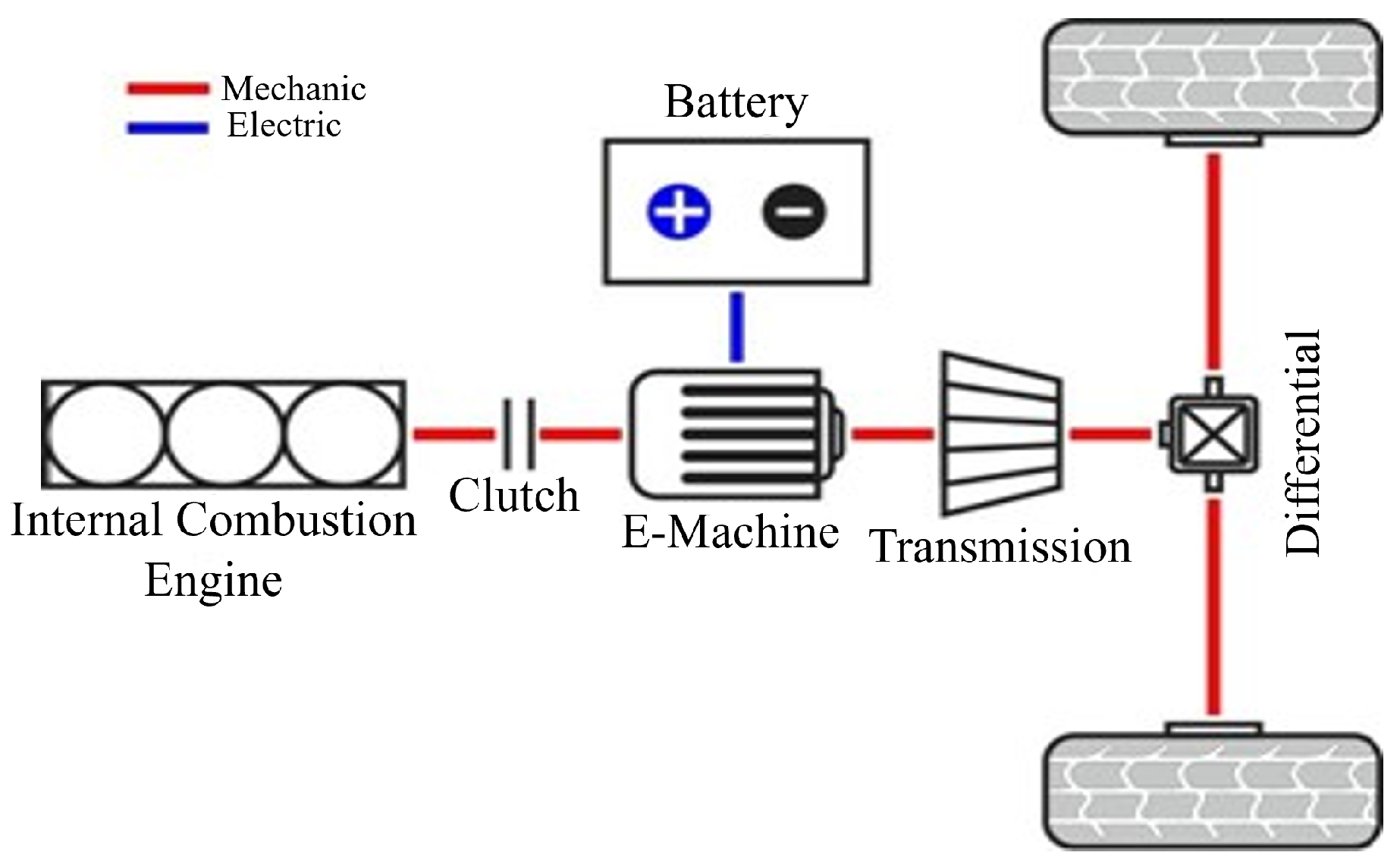
There are six main components of the powertrain, and they are the engine, clutch (separation clutch), EM, high-voltage battery, transmission, and differential. The connections, both mechanical and electrical, between these components are shown in Figure 1. The engine and EM are the two main traction sources of the vehicle and are placed on the same shaft. The energy transfer between these two components is bidirectional, as the battery supplies power to the EM during traction, and the opposite scenario holds during regenerative braking. The clutch, namely, the “separation clutch”, decouples the engine from the EM, which is the most characteristic feature of this hybrid architecture. The transmission includes a gearbox, where a related gear ratio is obtained, and the differential is the mechanical part where the rotational movement of the input shaft is transmitted to the wheels by considering the final drive ratio. P2 HEV architecture allows traction from the engine and EM separately or together based on driver request. Therefore, the most significant problem in achieving higher efficiency is the management of the torque distribution.

As a power source for electric motors, Li-On batteries offer great advantages. It is noteworthy that Li-On batteries, which have many advantages in specific energy, specific power, life span, cost, and performance criteria, are suitable for the automotive field [6,7,8].

The current, voltage, SOC, and energy capacity that a Li-On battery can provide are within certain limits. In Li-On batteries, the ranges of the current, voltage, and SOC play a big role in energy efficiency. For this reason, applications such as the SOC window have been developed, and studies have been conducted to establish more sensitive SOC estimation methods [9,10]. In addition, these values also change with the SOH. The SOH is one of the key concepts that need to be optimized, and it provides information about the health status and aging of the battery. Battery aging changes depend on the temperature, number of full cycles, battery chemistry, resistance, SOC status, and environmental conditions [11,12,13].

Various controllers are frequently used for the torque distribution problem, such as model predictive control (MPC), fuzzy logic, and reinforcement learning (RL).

Energy management strategies for HEVs are developed in [14] using fuzzy logic and Elman neural network tuning. The strategies aim to optimize the power split between the engine and electric motor by considering driving conditions, the battery state of charge, and other relevant factors. The fuzzy logic and Elman neural network tuning algorithms are compared with other energy management strategies using simulations.

The study in [15] compares two energy management strategies, fuzzy logic and the equivalent consumption minimization strategy (ECMS), for P2 HEVs. The strategies aim to optimize the power distribution between traction sources. A rule-based energy management strategy for a light-duty commercial P2 HEV using dynamic programming (DP) is presented in [16].

A two-level MPC approach for the energy management of parallel HEVs is proposed in [17]. The upper-level controller optimizes the power split between the engine, motor, and battery based on current driving conditions and driver demands. The lower-level controller implements the power split and manages the battery SOC. This approach enables the separate optimization of the energy management problem, uses simplified models for the powertrain components, and provides a more efficient and responsive system.

The study on the effect of SOC uncertainty on the MPC-based energy management strategy for HEVs in [18] examines the impact of uncertain SOC estimations on the performance of the MPC-based energy management strategy for HEVs. The study shows that higher levels of SOC uncertainty result in decreased fuel economy and increased battery degradation. Additionally, the study highlights the importance of accurate SOC estimations for optimal HEV performance and longevity.

An adaptive MPC strategy is proposed in [19], and it includes battery thermal limitations to optimize the fuel consumption of a P2 HEV. The proposed strategy considers the battery’s thermal behavior and adjusts the power distribution between the engine and electric motor to reduce fuel consumption while maintaining the battery’s thermal limits.

A hierarchical control strategy is proposed in [20] with a robust MPC for the energy management of parallel HEVs in the presence of uncertainty. The high-level controller is responsible for determining the setpoints of the low-level controller based on the driver demand and the vehicle’s operating conditions. The low-level controller is responsible for optimizing the energy flow between the powertrain components of the HEV based on the setpoints determined by the high-level controller.

A novel energy management strategy is proposed in [21] using a hierarchical MPC framework for plug-in HEVs. The study introduces a dynamic programming (DP) algorithm to solve the high-level MPC optimization problem efficiently. The DP algorithm optimizes the energy management strategy over the entire driving cycle and provides a set of optimal setpoints for the low-level controller to follow.

Using stochastic MPC and RL, the energy management of plug-in HEVs is analyzed in [22]. The proposed framework accounts for uncertainties in the PHEV’s operating conditions and uses a probabilistic model to solve a stochastic optimization problem. The study introduces an RL algorithm to learn the optimal control policy based on historical data, which significantly improves fuel economy compared to conventional rule-based strategies.

The main problem in MPC is the execution time of the controller due to its complex structure. To reduce execution frequency, many studies have been performed [23,24,25]. Triggering instances are determined based on the difference between the current measured state and the measurement in the previous sampling instance or the difference between the current measured state and the predicted optimal state [23,26,27,28,29].

The potential benefits of using event-triggered MPC strategies are demonstrated for BEVs and HEVs, including improved fuel economy, battery life, and reduced computational complexity, in [30,31,32]. MPC and DQN are different approaches and require different problem-solving methods. While MPC is used to create an optimized control strategy for a dynamic system, DQN combines the Q-learning algorithm with deep learning, allowing an agent to learn what actions to take to achieve the highest overall reward in a given environment. DQN is also used to solve the energy management problem in automotive applications in the literature [33,34].

Studies have been conducted to compare MPC and DQN [35]. In addition, there are studies in which the combination of MPC-DQN is used to increase the performance of MPC and to select design parameters, such as the prediction horizon and weight [36,37,38].

In this study, two nonlinear model predictive controllers are considered for different purposes. The first MPC provides the total torque request for reference velocity tracking under a finite prediction horizon according to the drivability criteria. The second MPC is applied under a finite prediction horizon to provide optimal torque distribution within the traction source limits. There are various physical limitations to the internal combustion engine, electric motor, and battery. Accordingly, the physical limits of the battery, voltage, and current can be applied between certain values. In addition, the working behavior of the battery changes with the aging of the battery. For this reason, the factors affecting the aging of the battery are taken into account. Finally, in order to decelerate the aging of the battery, the SOC window is determined, and the battery is set to operate between certain SOC values. The SOC and SOH concepts for torque distribution are taken into account with MPC.

The execution time of MPC can be considered a shortcoming to solve the complex optimal control problem in each step to provide a prediction control sequence. In this study, to reduce the frequency of solving the optimal control problem and to eliminate the mentioned problem, an event-triggered mechanism is constructed via DQN and integrated into MPC. In addition, due to the fact that the efficiency of the internal combustion engine, the electric motor, and the requested total torque change during driving, the weight terms of the cost function are intended to be modified adaptively. In order to achieve this, training with DQN is carried out, and appropriate weight terms are determined. In this way, the efficiency of energy consumption is improved with less frequency of operation of the controller.

This paper is organized as follows: In Section 2, the vehicle specifications, suitable battery/cell selection, and simulation and modeling environment are presented. In Section 3, the MPC methodology and vehicle dynamics are provided. In Section 4, the event-triggered mechanism and MPC weights via DQN are proposed. In Section 5, the results are provided and discussed, and Section 6 concludes this work.

2. Materials and Methods

A P2 HEV is modeled in the MATLAB/Simulink environment by using physical modeling, which contains Simscape™ blocks. This approach helps to integrate the specifications of the powertrain components and vehicle dynamics in such a way that they can be highly accurate. Additionally, three modeling standards, namely, MathWorks Advisory Board (MAB), Japan MATLAB Automotive Advisory Board (JMAAB), and Motor Industry Software Reliability Association (MISRA) 2012, are used to check that the vehicle model is built successfully. The results are created by using the MATLAB Model Advisor toolbox without fail. According to the publicly shared specifications of the P2 HEV Kia Niro, all vehicle components are modeled. The sampling time is chosen as 0.01 s as in most automotive applications.

The type of electric motor used in this vehicle is an Interior Permanent Magnet Synchronous Motor (IPMSM) and is often used in the automotive industry. The technical data, which comprise the type of motor, the maximum amount of torque, the maximum motor power, the operating voltage, the maximum speed, and the efficiency of the inverter and motor, are given in

Table 1. Powertrain specification of Kia Niro.

Specification
Motor Type	IPMSM
10 s Peak Power	32 kW
Maximum Torque	170 Nm
Maximum Speed	3750 min${}^{-1}$
System Nominal Voltage	240V
Motor Max. Efficiency	95%
Connected Inverter Efficiency	97%

. In addition to this information, an electric motor efficiency map based on the motor shaft speed and motor torque is also available. Since all the required parameters in the shared battery data are not available, battery pack and cell selections are made by taking into account the system configuration and motor performance criteria.

An automotive consists of many different components and subsystems. These components and subsystems combine to form a larger system that meets the functional requirements of the vehicle. However, managing all the systems of a vehicle as a whole is quite difficult and complex. Therefore, the system levels of the automotive industry are detailed from general to specific and provide the management of system requirements.

For the battery and cell, starting with L0 vehicle level requirements, L1 powertrain level, L2 battery level, and L3 module/cell level requirements are detailed. Finally, after checking whether the cell to be selected meets the high-level requirements, battery pack and cell selections are completed.

Starting from system level 1, the power of the battery should be calculated in charge and discharge cases based on the powertrain efficiency for battery selection. According to the inverter and electric motor efficiencies, the powertrain efficiency ratio is given in

Table 2. Powertrain element efficiency.

Inverter	Electric Motor	Powertrain
97%	95%	92.150%

.

With these efficiency values, when traction and recuperation such as regenerative braking are performed, the target power values of the battery in charge and discharge cases are as shown in

Table 3. Charging and discharging power.

Component	10 s Peak Discharging Power	10 s Peak Charging Power
Electric Motor	32 kW	32 kW
Battery	34.726 kW	29.488 kW

.

Afterward, a usable energy target which is shown in

Table 4. Usable energy target.

Criteria	Value	Unit
Target Range	6	km
Consumption	25	kWh/100 km
Consumption	250	Wh/km
Usable Target Energy	1500	Wh

is found over the estimated consumption values with the maximum range that can be reached in 1 battery cycle using only the motor for traction.

Another important criterion in determining battery cell is the chemistry of the battery. With different battery chemistries, the weight, cost, safety, performance, power, and voltage values of the battery vary. There are 6 different types of chemistries in frequently used Li-On batteries (

Table 5. Li-On battery chemistries [40].

Criteria	LCO	LMO	NMC	LFP	NCA	LTO
Nominal Voltage (V)	3.6	3.7	3.7	3.2	3.6	2.4
Specific Energy (Wh/kg)	150–200	100–150	150–220	90–120	200–260	50–80
Cycle Life	500–1000	300–700	1000–2000	2000–2500	500	3000–7000
Thermal Runaway (°C)	150	250	210	270	150	Safest

) [39,40].

Among other criteria, specific power and specific energy are evaluated as high priority, and NMC, which is the most widely used in the automotive industry, is selected as the battery chemistry. As the system level increases from 2 to 3, the serial–parallel configuration is determined by considering the battery’s chemistry and power demands. The cell nominal voltage of NMC, which is the chemistry of the selected battery, is 3.7 V. A total of 65 cells are needed to supply the system voltage. After determining the total number of cells that need to be connected in series, using the battery’s charge and discharge power values and system voltage values, the maximum charge and discharge requested currents of the battery are as follows:

$$\begin{array}{cc}\hfill {\displaystyle \frac{V_{Sys}}{V_{Cell}}}& \hfill =N_{Cell}⟶{\displaystyle \frac{240 \mathrm{V}}{3.7 \mathrm{V}}}\approx 65\hfill \end{array}$$

(1)

$$\begin{array}{cc}\hfill {\displaystyle \frac{P_{DisMax}}{V_{Sys}}}& \hfill =I_{DisMax}⟶{\displaystyle \frac{34.7 \mathrm{kW}}{240 \mathrm{V}}}=144.4 \mathrm{A}\hfill \end{array}$$

(2)

$$\begin{array}{cc}\hfill {\displaystyle \frac{P_{ChaMax}}{V_{Sys}}}& \hfill =I_{ChaMax}⟶{\displaystyle \frac{29.5 \mathrm{kW}}{240 \mathrm{V}}}=122.6 \mathrm{A}\hfill \end{array}$$

(3)

where V${}_{Sys}$ and V${}_{Cell}$ are the system and cell nominal voltage; N${}_{Cell}$ is the number of cells connected in series; and P${}_{DisMax}$, P${}_{ChaMax}$, I${}_{DisMax}$, and I${}_{ChaMax}$ are the 10 s peak discharge and charge power and current. By using 65 cells with a 3.7 V cell voltage, the battery can provide 240.5 V as the nominal voltage. After determining the use of 65 cells in series, the usable energy capacities are found to be 65s1p and 65s2p for the parallel configuration (

Table 6. Cell configuration.

Criteria	65s1p	65s2p
Battery Nominal Voltage	240.5 V	240.5 V
Usable Target Energy	1.5 kWh	1.5 kWh
Installed Target Energy	3 kWh	3 kWh
Used DOD	50%	50%
Cell Usable Energy Capacity (Ah)	6.237 Ah	3.118 Ah
Cell Installed Energy Capacity (Ah)	12.474 Ah	6.237 Ah

). The usable energy capacity of the battery is obtained by using the ratio of the usable target energy and the voltage. With the use of the SOC window, the energy capacity of the battery corresponds to separate values as installed and usable. There are various applications for using a battery pack for a long time or over a cycle to obtain consistent power without reducing its lifespan too much. One of them is to create an SOC window for SOC. The SOC window is intended to improve performance by operating the SOC in a narrower range rather than in the 0–100 range. The SOC window changes according to the structure and architecture of the vehicle. While this range is larger in electric vehicles, the SOC window is smaller in hybrid electric vehicles. It is needed to ensure that the battery is not used at very high and very low SOC percentages. High voltage values are required for a high SOC. In high-SOC situations, high voltage values stress the cell. For this reason, the life of the battery is reduced. Exceeding the maximum voltage limit represents a dangerous situation at high voltage, and it risks the safety of the cell and battery pack. For a low SOC, however, the open-circuit voltage values decrease, and the internal resistance increases. Thus, in the case of discharge, the voltage value may decrease further, and the minimum voltage limit may be exceeded. Due to all these reasons, the SOC is operated between 30% and 80%, and the SOC window is selected as 50% by examining other applications. The installed energy capacity of the battery is calculated by multiplying the usable energy capacity of the battery with the SOC window.

A battery with NMC chemistry that provides 12.474 Ah or 6.237 Ah cell-installed energy capacity (Ah) and can deliver more than the desired current values should be selected. Batteries, which are frequently used in the automotive industry and are the subject of long-term tests, are examined, and a battery that meets the system requirements is selected. The battery specifications are shown below (

Table 7. Verification of the battery pack for system requirements.

Specification	Battery	System Requirement
Configuration	65s2p	-
Cell Nominal Voltage (V)	3.71	3.7
Pack Nominal Voltage (V)	241.15	240
Cell Usable Energy (Ah)	6.73	6.237
Cell Installed Energy (Ah)	13.46	12.474
SoC Window	30–80%	30–80%
Used SOC	50%	50%
Usable Energy (kWh)	1.6229	1.5
Installed Energy (kWh)	3.245	3

).

It is seen that the usable energy capacity, required current limits, and voltage values, which are system requirements, are provided with the characteristics of the selected battery.

3. System Dynamics and Prediction Model

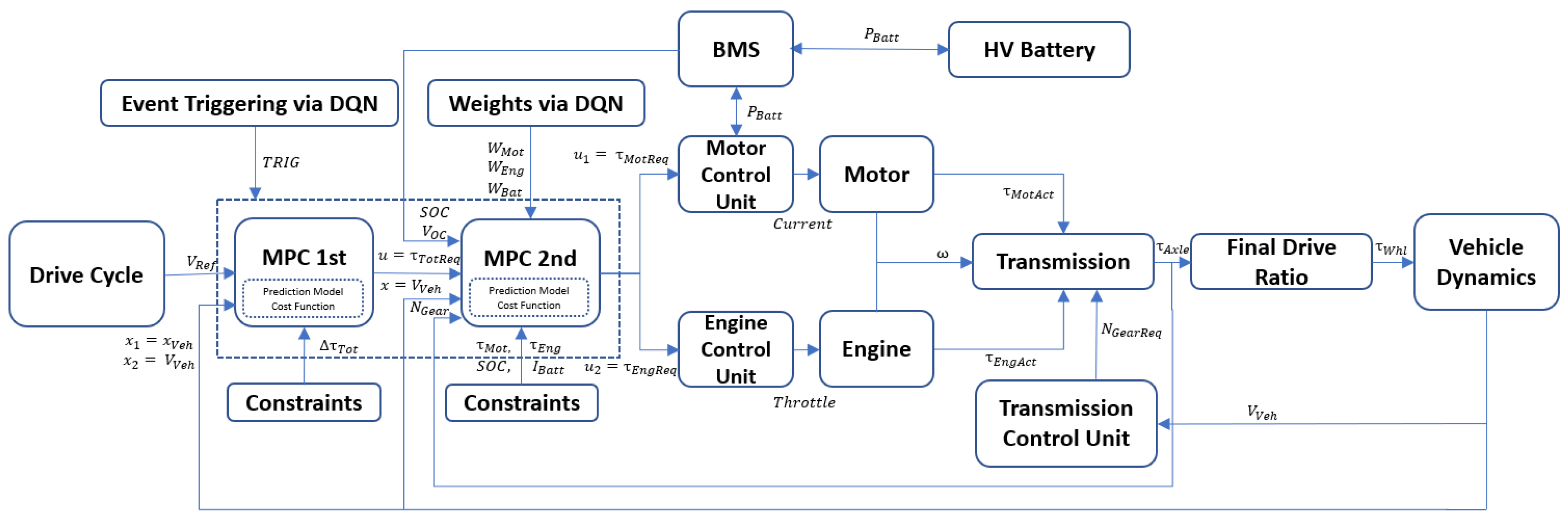
In this section, the flow diagram of the study (which can be seen in Figure 2), vehicle dynamics equations, and relations for nonlinear model predictive control are explained.

As can be seen in Figure 2, while tracking the Worldwide Harmonized Light Vehicle Test Procedure (WLTP) velocity reference and distributing the torque between the engine and motor, two MPCs are integrated into the powertrain system, and they dynamically adjust the torque to optimize performance and efficiency.

The first MPC calculates the total torque request, which is the control signal u, based on the WLTP velocity reference V${}_{Ref}$, vehicle position x${}_1$, and velocity x${}_2$ by considering drivability. The total torque request is the setpoint of the second MPC. The requested total torque is distributed between the engine and motor based on a number of constraints, such as the SOC, engine torque limits, motor torque limits, and battery current I${}_{Batt}$ via the second MPC. The distribution of the torque is adjusted continuously based on feedback from the vehicle velocity, SOC level, open-circuit voltage, and actual gear.

The requested torque outputs ${\tau }_{MotReq}$ and ${\tau }_{EngReq}$ of the powertrain system are controlled and regulated by various components, such as the engine control unit (ECU), the motor control unit (MCU), and the transmission control unit (TCU). After that, the produced torques, which are ${\tau }_{MotAct}$ and ${\tau }_{EngAct}$, are typically transmitted to the wheels as ${\tau }_{Axle}$ and ${\tau }_{Whl}$ via the transmission and final drive ratio, respectively. In an HEV, the electric motor is powered by a battery pack, which provides electrical energy to the motor. The current flow in the powertrain system refers to the flow of electrical power $P_{Batt}$ from the battery to the motor, as well as the flow of energy back to the battery during regenerative braking. The current is controlled and regulated by the battery management system (BMS), which adjusts the voltage and current supplied to the motor based on the desired torque output and other factors. The event-triggered mechanism via DQN and the weights of the second MPC via DQN are integrated to increase the efficiency of the MPCs.

In this study, two MPCs are integrated to obtain the optimal solution. Using two MPCs instead of one complex MPC has advantages in systems with many constraints. With regard to improving performance and feasibility, in systems with many constraints, it can be challenging to find a solution that satisfies all constraints. By using two simple MPC controllers, each controller can focus on a subset of constraints, making it easier to find feasible solutions that satisfy all constraints. Additionally, reducing computational complexity is another aim. When there are many constraints, a complex MPC controller may require a large number of optimization variables, resulting in high computational complexity. By using two simple MPC controllers, each controller can focus on a smaller set of optimization variables, reducing the overall computational complexity of the control system. Lastly, each controller can be designed to optimize different aspects of the control performance, providing greater flexibility in the control system.

For the prediction model, resistance forces, which are given in Equation (7), affect the vehicle in the opposite direction depending on vehicle velocity, mass, frontal area, etc. Basically, there are three main resistances forces that are applied to the vehicle.

$$\begin{array}{cc}\hfill F_{AirR}& \hfill =0.5\rho c_d{A}_v{V}^2\hfill \end{array}$$

(4)

$$\begin{array}{cc}\hfill F_{GradR}& \hfill =mgsin\left(\theta \right)\hfill \end{array}$$

(5)

$$\begin{array}{cc}\hfill F_{RollR}& \hfill =mg{c}_r\hfill \end{array}$$

(6)

$$\begin{array}{cc}\hfill F_{TotR}& \hfill =F_{AirR}+F_{GradR}+F_{RollR}\hfill \end{array}$$

(7)

By taking into consideration the road gradient, wind speed, and mechanical motion, the resistance forces are calculated in the prediction model to generate a control signal in order to track the reference input.

With the first MPC, the total torque request should provide the traction forces not only for all resistance forces but also for the velocity tracking error between the vehicle velocity and reference velocity. The nonlinear model equations are as follows:

$$\begin{array}{cc}\hfill F_{Req}& \hfill ={\displaystyle \frac{({\tau }_{Mot}+{\tau }_{Eng}+\Delta {\tau }_{Tot})N_{Gear}{N}_{FDR}}{r}}\hfill \end{array}$$

(8)

$$\begin{array}{cc}\hfill F_{Net}& \hfill =F_{Req}-F_{TotR}\hfill \end{array}$$

(9)

$$\begin{array}{cc}\hfill {\dot{x}}_1& \hfill =x_2\hfill \end{array}$$

(10)

$$\begin{array}{cc}\hfill {\dot{x}}_2& \hfill ={\displaystyle \frac{F_{Net}}{m}}\hfill \end{array}$$

(11)

$$\begin{array}{cc}\hfill x_2(k+1)& \hfill =x_2\left(k\right)+{\displaystyle \frac{F_{Net}{T}_s}{m}}\hfill \end{array}$$

(12)

$$\begin{array}{cc}\hfill x_1(k+1)& \hfill =x_1\left(k\right)+x_2(k+1)T_s\hfill \end{array}$$

(13)

where $\Delta {\tau }_{Tot}$ is the control signal, which is the requested total delta torque. x${}_1$ and x${}_2$ are system states, which are the position and vehicle velocity. The axle-based torque values ${\tau }_{Mot}$ and ${\tau }_{Eng}$ are transmitted to the wheel-based torque via the powertrain components, which are the transmission and final drive ratio. The wheel-based torque is converted to the requested force by dividing the wheel radius. x${}_1$ is updated by considering the net force and vehicle mass, which correspond to acceleration. For the vehicle dynamics of P2 HEV, the nomenclature is given in

Table 8. Nomenclature.

Variable	Description
F${}_{TotR}$	Total resistance force
F${}_{AirR}$	Aerodynamic resistance force
F${}_{GradR}$	Grade resistance force
F${}_{RollR}$	Rolling resistance force
F${}_{Req}$	Force requested by driver
F${}_{Net}$	Net force
${\tau }_{Eng}$	Engine-based torque
${\tau }_{Mot}$	Motor-based torque
$\rho$	Air density
c${}_d$	Drag coefficient
A${}_f$	Vehicle frontal areal
V	Vehicle velocity
m	Vehicle mass
g	Gravity
$\theta$	Road angle
C${}_r$	Rolling resistance coefficient
N${}_{Gear}$	Gear ratio
N${}_{FDR}$	Final drive ratio
r	Wheel radius

.

The limit of motion, as defined in the ISO 2631-5 standard (

Table 9. ISO 2631-5 acceleration limits [41].

Comfort Levels	Acceleration Limits
Not uncomfortable	0.315 m/s${}^2$
A little uncomfortable	0.63 m/s${}^2$
Fairly uncomfortable	1.0 m/s${}^2$
Uncomfortable	1.6 m/s${}^2$
Very uncomfortable	2.5 m/s${}^2$

) [41], is a measure of the maximum displacement of a vehicle’s body or chassis experienced by the driver or passengers during normal driving conditions. It is expressed as a percentage of the total body or chassis displacement and is used to evaluate the drivability of a vehicle. The limit of motion can significantly affect the comfort and safety of the vehicle’s occupants, with vehicles with a lower limit of motion typically being more stable and comfortable to drive. However, vehicles with a higher limit of motion may be more prone to vibrations and other movements that can be unsettling for the driver and passengers.

According to the ISO 2631-5 standard, comfort levels are given according to the acceleration values. Torque demands and torque variation occur in line with acceleration changes. In order for the requested torque and requested torque changes to be realizable, the acceleration changes specified in the standard are taken as a reference. Using the acceleration–torque relationship, the torque variation limits are determined as follows:

$$\begin{array}{cc}\hfill F& \hfill =ma\hfill \end{array}$$

(14)

$$\begin{array}{cc}\hfill a& \hfill ={\displaystyle \frac{\Delta {\tau }_{Tot}{N}_{Gear}{N}_{FDR}}{rm}}\hfill \end{array}$$

(15)

$$\begin{array}{cc}\hfill \Delta {\tau }_{Tot}^{Low}& \hfill <\Delta {\tau }_{Tot}<\Delta {\tau }_{Tot}^{Upp}\hfill \end{array}$$

(16)

where $\Delta {\tau }_{Tot}^{Low}$ and $\Delta {\tau }_{Tot}^{Upp}$ are the control signal upper and lower limits, which correspond to the ISO 2631-5 acceleration limits. For the total torque request, the cost function is established as follows:

$$\begin{array}{c}\hfill J=\sum _{j=1}^N{W}_{Track}\left(x_{2Ref}(k+j|k)\right)-x_2{(k+j|k))}^2\end{array}$$

(17)

where N is the prediction horizon, W${}_{Track}$ is the tracking weight, and x${}_{2Ref}$ is the reference velocity for a given discrete time step k. After calculating the requested total engine and motor torques, one must calculate how much torque should be demanded and from which traction source for minimum power consumption. In HEVs, the torque distribution between the engine and the motor can have a significant impact on the vehicle’s performance and fuel efficiency. The engine and motor can work together to provide the necessary power to the vehicle, or they can operate independently to optimize efficiency.

For example, in a hybrid electric vehicle, the engine may be used to power the car at higher speeds, while the electric motor is used at lower speeds or during acceleration to provide additional torque. This can help to reduce the workload on the engine and improve fuel efficiency. Similarly, the electric motor may be used to power the vehicle during stop-and-go traffic or at low speeds, which can help to reduce fuel consumption and emissions.

Variations of motor torque and engine torque are selected as control signals. The aim of the selection of the delta motor and engine torque as control signals is to prevent steady-state errors by using integral action. The equality constraint is applied in order to be able to generate the requested torque for the HEV in Equation (18).

$$\begin{array}{c}\hfill {\tau }_{Tot}=(u_1+{\tau }_{Mot})+(u_2+{\tau }_{Eng})\end{array}$$

(18)

Powertrain components work within the limited operating range inherently; hence, the limits of the motor, engine, battery, and associated system variables are taken into consideration for the controller design.

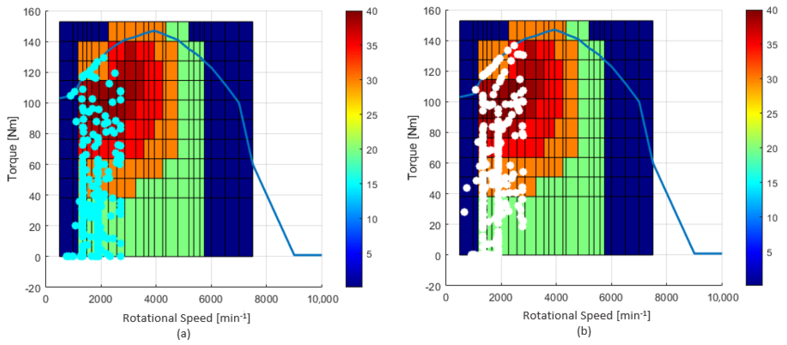
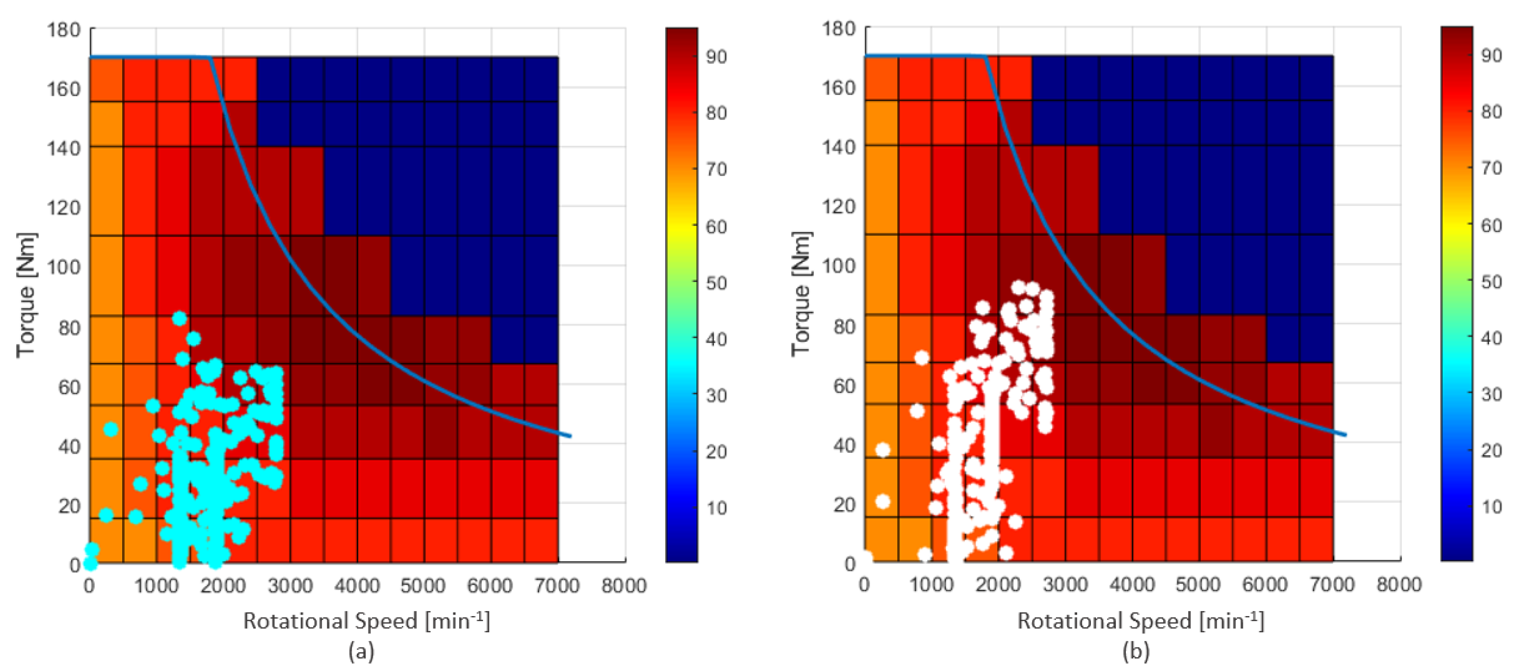
Figure 3a,b show the characteristics of the engine and motor, respectively. The blue lines represent the rotational speed and torque curves. These torque curves are the physical limits of the engine and motor; hence, they are used as MPC constraints. The colored regions show the engine and motor efficiency, which takes the values shown on the efficiency bar.

For the torque constraints, the rotational speed is calculated via the vehicle speed dynamically.

$$\begin{array}{c}\hfill {\omega }_{Mot}={\omega }_{Eng}={\displaystyle \frac{x_2{N}_{Gear}{N}_{FDR}}{0.3769r}}\end{array}$$

(19)

The engine and motor constraints for the HEV are considered with the following equations:

$$\begin{array}{cc}\hfill {\tau }_{Eng}^{Upp}& \hfill =interpl({\omega }_{Eng}^{Axis},{\tau }_{Eng}^{Axis},{\omega }_{Eng})\hfill \end{array}$$

(20)

$$\begin{array}{cc}\hfill {\tau }_{Mot}^{Upp}& \hfill =interpl({\omega }_{Mot}^{Axis},{\tau }_{Mot}^{Axis},{\omega }_{Mot})\hfill \end{array}$$

(21)

$$\begin{array}{cc}\hfill {\tau }_{Eng}^{Low}& \hfill =0\hfill \end{array}$$

(22)

$$\begin{array}{cc}\hfill {\tau }_{Mot}^{Low}& \hfill =-{\tau }_{Mot}^{Upp}\hfill \end{array}$$

(23)

$$\begin{array}{cc}\hfill {\tau }_{Eng}^{Low}& \hfill <{\tau }_{Eng}<{\tau }_{Eng}^{Upp}\hfill \end{array}$$

(24)

$$\begin{array}{cc}\hfill {\tau }_{Mot}^{Low}& \hfill <{\tau }_{Mot}<{\tau }_{Mot}^{Upp}\hfill \end{array}$$

(25)

where ${\tau }_{Eng}^{Upp}$, ${\tau }_{Eng}^{Low}$, ${\tau }_{Mot}^{Upp}$, and ${\tau }_{Mot}^{Low}$ are the upper and lower limits of the engine and motor. The axis values of the engine and motor, which are taken from the vehicle datasheet, are predefined to generate limit curves via interpolation. According to the axis values of the torque and rotational speed, the upper limits of the engine and motor are determined based on the actual rotational speed by interpolating. The engine cannot produce negative torque, but the motor can work as a generator to charge a battery, so the lower limit of the engine is 0, and the lower limit of the motor is the negative sign of the upper limit.

In order to provide the torque to be demanded from the motor, the battery must provide a current. The relationship between the battery current and motor torque indicating motor efficiency can be used to calculate the required battery current.

$$\begin{array}{cc}\hfill Mo{t}_{Eff}& \hfill ={\displaystyle \frac{{\omega }_{Mot}{\tau }_{Mot}}{I_{Batt}{V}_{Batt}9.5488}}\hfill \end{array}$$

(26)

$$\begin{array}{cc}\hfill I_{Batt}& \hfill ={\displaystyle \frac{{\omega }_{Mot}{\tau }_{Mot}}{Mo{t}_{Eff}{V}_{Batt}9.5488}}\hfill \end{array}$$

(27)

The motor torque can be represented by the control signal, while the motor speed in the next sample is obtained via the vehicle speed using Equation (19). Motor efficiency is calculated with a lookup table that includes the motor torque and motor speed.

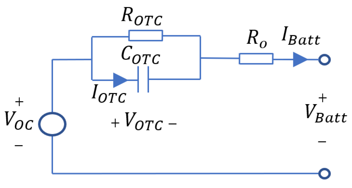
The voltage can be found in the battery equivalent circuit depending on the current with the ohmic resistance, open-circuit voltage, and RC pair, which shows Butler–Volmer effects or the double-layer effect. The double-layer effect is a phenomenon that occurs at the interface between a solid and a liquid (such as an electrode and an electrolyte). It is caused by the presence of a thin layer of charges at the interface, which can be either positive or negative depending on the materials involved. This thin layer of charges, known as the electric double layer, can have a significant effect on the overall behavior of the system. The double-layer effect behavior is similar to that of the capacitor [42]. The Butler–Volmer equation is a mathematical expression that describes the current flowing through an electrode–electrolyte system in terms of the overpotential (a measure of the driving force for the reaction) and the exchange current density (a measure of the rate at which the reaction occurs). The equation takes into account the effect of the electric double layer on the overall behavior of the system and can be used to predict the behavior of electrochemical cells under various conditions [43]. In light of this information, the battery equivalent model is given in Figure 4, and the mathematical equations of battery are as follows:

$$\begin{array}{cc}\hfill V_{OTC}(k+1)& \hfill =V_{OTC}\left(k\right)+\left(1-e^{{\displaystyle \frac{-T_s}{{\tau }_{OTC}}}}\right)\hfill \end{array}$$

(28)

$$\begin{array}{cc}\hfill V_{Batt}& \hfill =V_{OC}\left(SOC\right)-V_{OTC}-R_o{I}_{Batt}\hfill \end{array}$$

(29)

where V${}_{OTC}$ is the one-time constant voltage for the RC pair, ${\tau }_{OTC}$ is the time constant of the RC pair used to represent the double-layer effect, R${}_o$ is the ohmic resistance, V${}_{Batt}$ is the battery voltage, and V${}_{OC}$(SOC) is the open-circuit voltage. The open-circuit voltage has different behaviors according to the charge and discharge conditions. In the open-circuit voltage change, the charging and discharging speeds can be different due to different current values. The charging rate of the battery is denoted by C as shown below. For example, if a battery with a capacity of 6.5 Ah is charged with 13 A, it is charged in half an hour and charged with 2C.

$$\begin{array}{cc}\hfill C& \hfill ={\displaystyle \frac{I_{Batt}}{Q_{Max}}}\hfill \end{array}$$

(30)

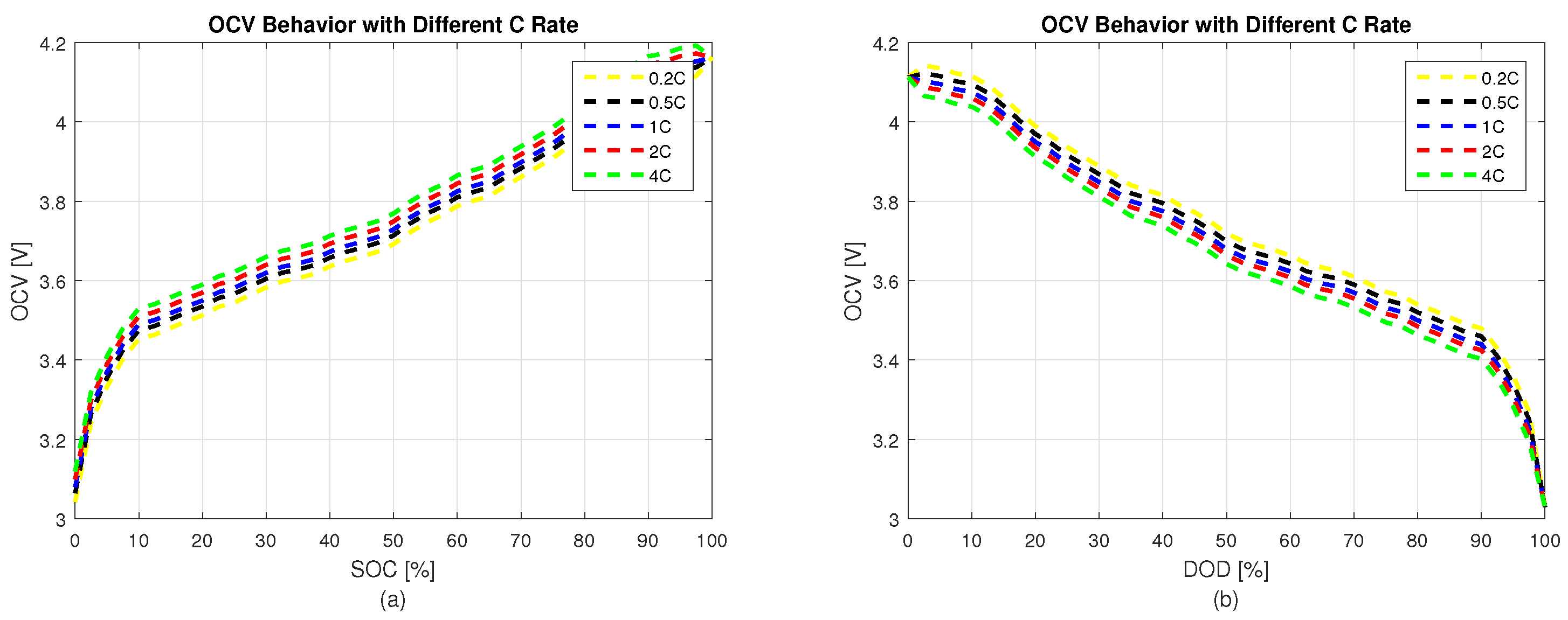
V${}_{OC}$(SOC) is calculated according to the curves presented in Figure 5.

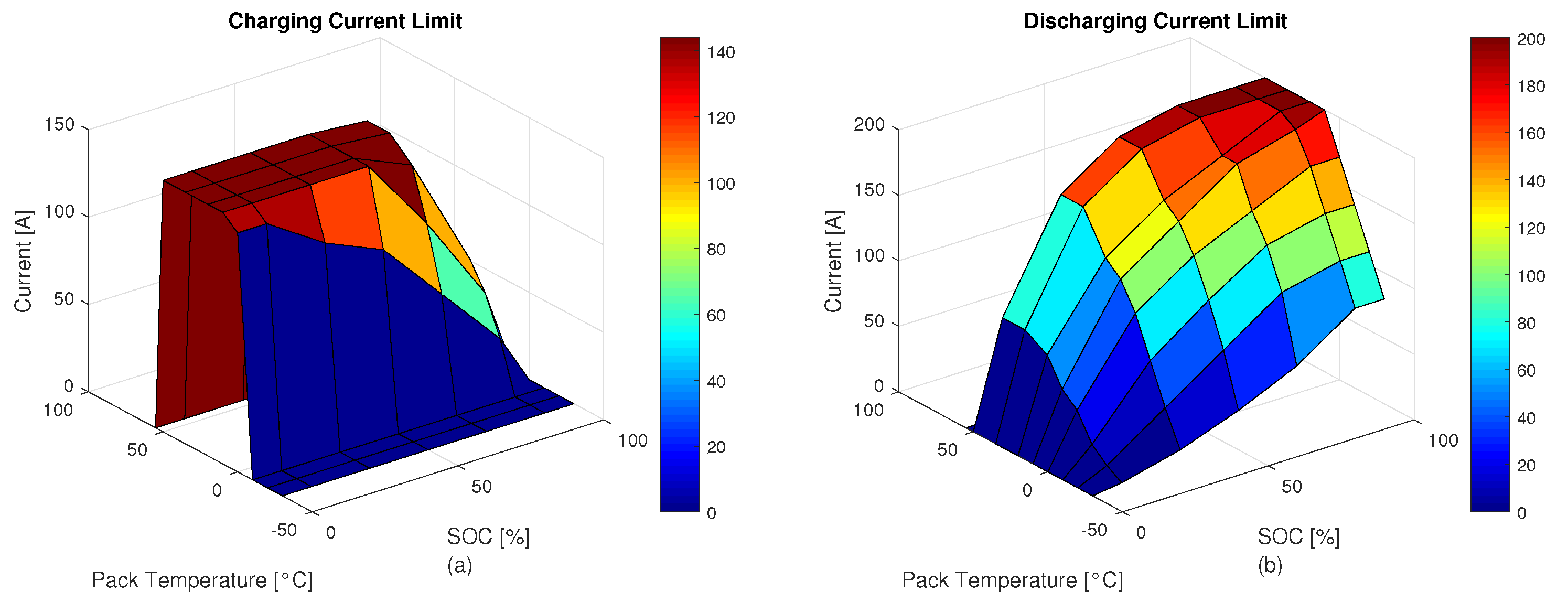
Another electrochemical event is the mass transport or Warburg effect. Since long periods such as minutes or hours are required to observe mass transport or Warburg effects, the same battery circuit model is used like many commercial vehicles’ battery models, and this effect has been ignored. The battery current varies with the pack temperature and SOC value. The currents that can be provided by considering these variables differ in charge and discharge processes. In the model used, the battery temperature is assumed to be constant at 25 °C; in this way, a three-dimensional representation which is given in Figure 6 becomes a two-dimensional representation.

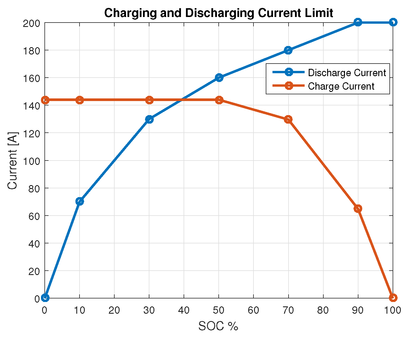
In Figure 7, the maximum current limits that can be given depending on the SOC and constant temperature are given according to the charge discharge.

$$\begin{array}{cc}\hfill I_{Batt}^{Low}& \hfill <I_{Batt}<I_{Batt}^{Low}\hfill \end{array}$$

(31)

The charge current represents a positive value, while the discharge current represents a negative value. For this reason, the discharge current limit is shown as the lower limit, and the charging current is shown as the upper limit.

The SOC variation is determined using the ratio of the battery current to the rated capacity. The SOC is calculated by adding the SOC variation to the initial SOC value.

$$\begin{array}{cc}\hfill SOC(k+1)& \hfill =SOC\left(k\right)-{\displaystyle \frac{\eta I_{Batt}\left(k\right)T_s}{Q_{max}}}\hfill \end{array}$$

(32)

where SOC$\left(k\right)$ is the initial SOC, I${}_{Batt}$ is the battery current, and $\eta$ is the cell coulombic efficiency in the charge phase [44].

The initial value of the SOC and the regular current measurements are very important in this method. Although it is a very widely used method, calendar aging should be taken into account in the calculation of the initial SOC value, and the effects of the SOH on Q${}_{max}$ should be taken into account.

The Q${}_{max}$ capacity value changes with the SOH effects. As a rule of thumb, when the capacity of a battery drops to 80%, it is assumed that the battery has reached the end of its life for automotive applications. For this reason, the aging effects of the battery are examined between 100% and 80% of the SOH value. The investigated effects are cyclic effects and temperature effects.

Each charge and discharge of the battery is shown as one cycle. The aging of the battery increases with each cycle. This cycling effect also changes with the use of the SOC window.

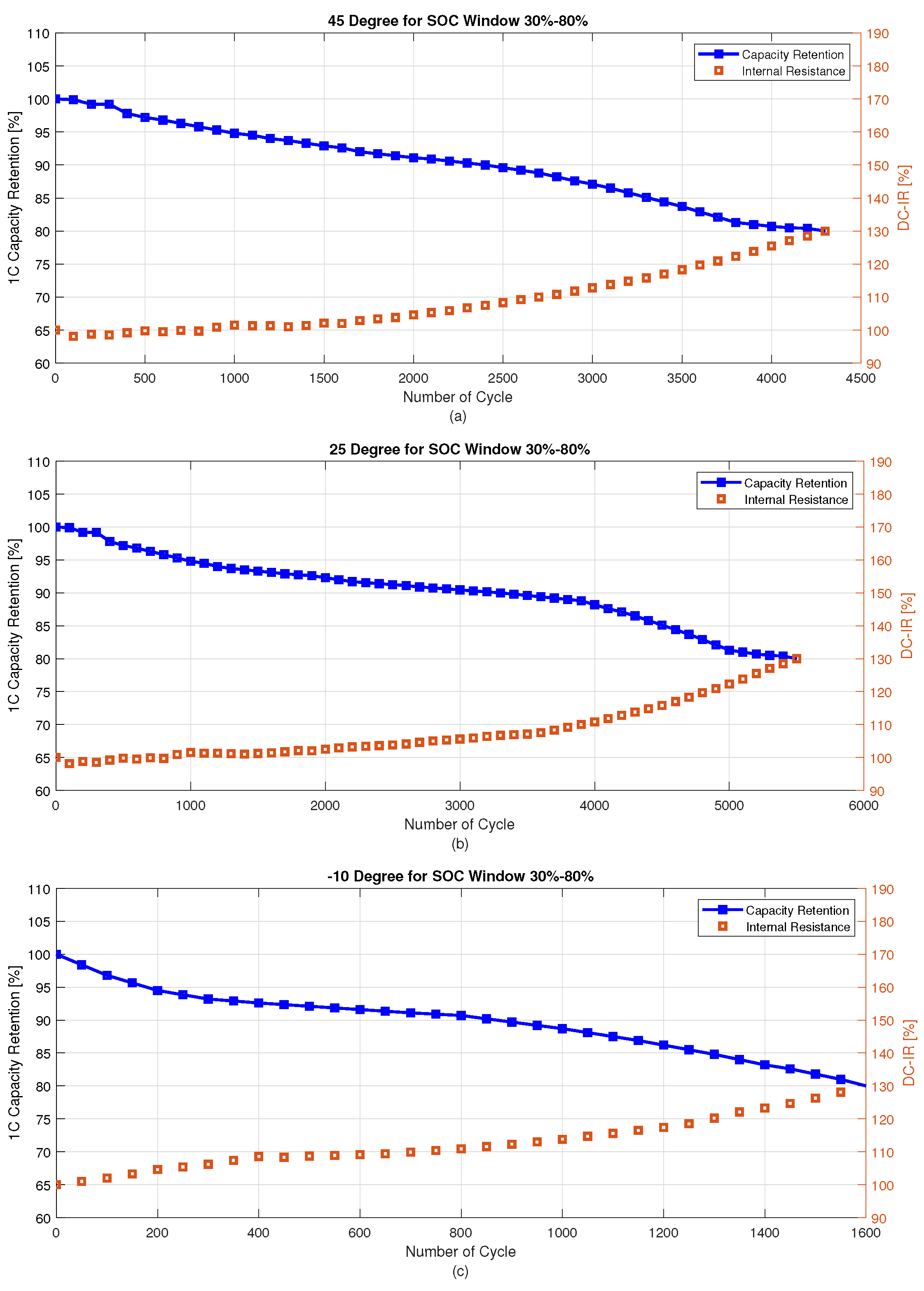
Cell temperature, which is another factor, can have a significant effect on the SOH of a battery. High temperatures can accelerate the degradation of the battery, reducing its overall lifespan and performance. This is because high temperatures can cause chemical reactions to occur within the battery at a faster rate, leading to increased chemical breakdown. However, low temperatures can also have a negative impact on the battery SOH by slowing down the battery’s chemical reactions and reducing its performance. This can lead to a decrease in battery capacity and overall lifespan. To show the cell temperature at −10${}^{\circ }$, 25${}^{\circ }$, and 45${}^{\circ }$ and the number of cycle effects, the capacity retention and internal resistance change are given below.

According to Figure 8, the SOH function is created based on the number of cycles and cell temperature in Equation (33).

$$\begin{array}{cc}\hfill SOH\%& \hfill =f(N_{Cyc},T_{Cell})\hfill \end{array}$$

(33)

Q${}_{max}$ is updated via the lookup table based on the effects of cycling N${}_{Cyc}$ and the T${}_{Cell}$ temperature. Thus, the accuracy of the estimation is increased by using the SOH effects given in Equation (33) in the SOC estimation.

The SOC window is important for managing the battery’s SOC within a safe and optimal range. The battery may be operated at either very high or very low SOC levels, which can lead to accelerated degradation, reduced performance, and safety hazards, which are explained in Section 2. By selecting an appropriate SOC window, one can maintain the battery within a safe and effective operating range, prevent overcharging or deep discharge, avoid thermal runaway, and prolong the battery’s useful life; hence, the SOC is requested to operate in this operating range and is added as a constraint to the MPC. The SOC window and MPC constraint are shown in Figure 9.

$$\begin{array}{cc}\hfill SO{C}_{Low}& \hfill <SOC<SO{C}_{Upp}\hfill \end{array}$$

(34)

$$\begin{array}{cc}\hfill 30& \hfill <SOC<80\hfill \end{array}$$

(35)

A lower power consumption indicates a lower power loss. For this reason, the cost function is as follows:

$$\begin{array}{c}\hfill J=\sum _{j=1}^N{W}_{Eng}\left(En{g}_{Loss}(k+j|k)\right)+W_{Mot}\left(Mo{t}_{Loss}(k+j|k)\right)+W_{Batt}\left(Bat{t}_{Loss}(k+j|k)\right)\end{array}$$

(36)

where W${}_{Mot}$, W${}_{Eng}$, and W${}_{Batt}$ are weighted coefficients for the state and control signal. Additionally, the motor, engine, and battery losses are represented as follows:

$$\begin{array}{cc}\hfill Mo{t}_{Loss}& \hfill ={\tau }_{Mot}\left(k\right){\omega }_{Mot}\left(k\right)=u_1{\omega }_{Mot}\left(k\right)\hfill \end{array}$$

(37)

$$\begin{array}{cc}\hfill En{g}_{Loss}& \hfill ={\tau }_{Eng}\left(k\right){\omega }_{Eng}\left(k\right)=u_2{\omega }_{Eng}\left(k\right)\hfill \end{array}$$

(38)

$$\begin{array}{cc}\hfill Bat{t}_{Loss}& \hfill =I_{Batt}\left(k\right)V_{Batt}\left(k\right)\hfill \end{array}$$

(39)

All constraints for the torque distribution are as follows:

$$\begin{array}{cc}\hfill {\tau }_{Tot}& \hfill =(u_1+{\tau }_{Mot})+(u_2+{\tau }_{Eng})\hfill \end{array}$$

(40)

$$\begin{array}{cc}\hfill {\tau }_{Eng}^{Low}& \hfill <{\tau }_{Eng}<{\tau }_{Eng}^{Upp}\hfill \end{array}$$

(41)

$$\begin{array}{cc}\hfill {\tau }_{Mot}^{Low}& \hfill <{\tau }_{Mot}<{\tau }_{Mot}^{Upp}\hfill \end{array}$$

(42)

$$\begin{array}{cc}\hfill I_{Batt}^{Low}& \hfill <I_{Batt}<I_{Batt}^{Low}\hfill \end{array}$$

(43)

$$\begin{array}{cc}\hfill SO{C}_{Low}& \hfill <SOC<SO{C}_{Upp}\hfill \end{array}$$

(44)

4. MPC Event-Triggered and Weight Adaptation Mechanism

4.1. Training of Event-Triggered Mechanism

In the HEV, the event-triggered mechanism via DQN is implemented in the MPCs for the velocity tracking system.

Event-triggered MPC has several advantages over traditional MPC. First, it can reduce the computational burden of the control algorithm, as the control action is only updated when necessary. This can be particularly important in systems with limited computing resources or in applications where frequent updates of the control action are not required. Second, event-triggered MPC can improve control performance by ensuring that the control action is updated in response to significant changes in the system behavior rather than continuously updating the control action regardless of the system state. This can result in a more efficient and effective control strategy, especially for systems with nonlinear or time-varying dynamics. To realize the event-triggered mechanism, DQN is used.

The goal of realizing the event-triggered mechanism via DQN is to learn the optimal control policy that maximizes the expected cumulative reward over a finite time horizon, given the current state s${}_k$ of the system. In the event-triggered DQN, the Q-function Q$(s,a)$ is used to approximate the expected cumulative reward of taking action a in state s and following the optimal control policy thereafter:

$$\begin{array}{cc}\hfill Q_{\pi }^{*}(s,a)& \hfill =maxE[\sum _{k=1}^{\infty }{\gamma }^{k}r(s_k,a_k)|s_0=s,a_0=a;\pi ]\hfill \end{array}$$

(45)

where r is the reward at time k, which is a function of the state s${}_k$ and the control action a${}_k$. The Q-function is updated as follows:

$$\begin{array}{c}\hfill Q(s,a)⟵Q(s,a)+\alpha (r+\gamma maxQ(s^{\prime },a^{\prime })-Q(s,a))\end{array}$$

(46)

where r$(s,a)$ is the immediate reward for taking action a in state s; $s^{\prime }$ is the next state; and $\alpha$ and $\gamma$ are the learning rate and discount factor, respectively. The learning rate and discount factor are two important hyperparameters that affect how the agent learns and makes decisions. The learning rate determines the step size at each iteration of the Q-learning algorithm, which updates the Q-values of the state–action pairs based on the rewards received by the agent. The discount factor determines the importance of future rewards in the agent’s decision-making process. It determines how much the agent values immediate rewards versus long-term rewards.

The main aim is to track the velocity reference with less triggering. To track the velocity reference, states, and action are determined as follows:

$$\begin{array}{cc}\hfill s_j& \hfill =\sum _{j=0}^3{V}_{ref}(k+j)-V\left(k\right)\hfill \end{array}$$

(47)

$$\begin{array}{cc}\hfill a& \hfill =[0,1]\in Z\hfill \end{array}$$

(48)

The states are determined as the difference between the vehicle velocity and forward-first four reference velocity values. For the triggering mechanism, an action set consists of “0 and 1”, where 0 means no triggering, and 1 means triggering.

One of the essential topics is the reward for DQN. A reward is a metric that tells the system how well it is performing. It can serve to maximize gains, minimize losses, etc., but the general goal is to maximize the total rewards over time. To fulfill the objective, the reward is determined based on the tracking ability and triggering.

$$\begin{array}{cc}\hfill r_1& \hfill =-|\sum _{j=0}^3{V}_{ref}(k+j)-V\left(k\right)|w_1\hfill \end{array}$$

(49)

$$\begin{array}{c}\hfill r_2=\left\{\begin{array}{cc}(Li{m}_V-|\sum _{j=0}^3{V}_{ref}(k+j)-V\left(k\right)\left|\right)w_2,\hfill & \mathrm{if}|\sum _{j=0}^3{V}_{ref}(k+j)-V\left(k\right)|\le Li{m}_V\hfill \\ 0,\hfill & \mathrm{otherwise}\hfill \end{array}\right.\end{array}$$

(50)

$$\begin{array}{cc}\hfill r_3& \hfill =-a_k{w}_3\hfill \end{array}$$

(51)

$$\begin{array}{cc}\hfill r_k(s,a)& \hfill =r_1+r_2+r_3\hfill \end{array}$$

(52)

where w${}_1$ and w${}_3$ are weight calibration parameters, and w${}_2$ is the calibration lookup table used to calibrate the reward function. The first term of the reward is the state difference reward. It is used as a punishment from a technical point of view. In the case of a higher state difference, the punishment increases based on the quantity of the state difference between the vehicle velocity and vehicle velocity forward-first four references.

The second term of the reward is the track reward. The second reward term is related to the first reward term, and if the difference between the vehicle speed and the first four velocity reference values is lower than a certain parameter Lim${}_V$, it gives the reward a positive value according to the velocity difference and 1D lookup table. Otherwise, no rewards are given.

The third reward term is related to triggering. The goal is to perform velocity tracking with minimal triggering. For this reason, a penalty value is applied in the case of triggering.

There are few ways to determine the neuron size and hidden layer number based on experiments, intuition, and literature studies. The neuron size, hidden layer size, and activation function type are determined based on trial and error. The activation function is selected as the rectified linear unit (RELU), the hidden layer number is determined to be 3, and the neuron size is selected to be 24 empirically. The working condition of the event-triggered mechanism is that the DQN output is greater than 0.5.

The world, real or virtual, in which the agent performs actions when the reinforcement system begins exploring its environment, is entirely unaware of this system behavior. By observing the results, it gains more experience. The exploration vs. exploitation trade-off is typically controlled by an epsilon-greedy policy. During training, the agent selects the action with the highest Q-value with probability 1 − $ϵ$ and selects a random action with probability epsilon. This way, the agent can balance the need to explore and the need to exploit.

$$\begin{array}{c}action=\left\{\begin{array}{cc}Randomaction,\hfill & ϵ\hfill \\ maxQ(s,a),\hfill & \hfill 1-ϵ\hfill \end{array}\right.\hfill \end{array}$$

(53)

where $ϵ$ is a hyperparameter that controls the trade-off between exploration and exploitation in the agent’s decision-making process. Moreover, $ϵ$ is updated as follows:

$$\begin{array}{cc}\hfill ϵ& \hfill =ϵ(1-{ϵ}_{decay})\hfill \end{array}$$

(54)

With every episode, the epsilon value decays by using ${ϵ}_{decay}$, which is the epsilon decay parameter. In this way, in the first phase of training, the agent explores the environment. By decreasing the epsilon value, the agent exploits and gains more rewards. Finally, for training, the MATLAB Reinforcement Learning Toolbox is used.

4.2. Training for Adaptation of Weights of MPC’s Cost Function

For this section, the cost function of the weight terms updated with DQN is employed. The main advantage of using DQN for MPC weight training is that it can handle complex, high-dimensional state and action spaces that may be difficult to optimize using traditional optimization techniques. DQN can learn an optimal policy by approximating the Q-value function, which is a measure of the expected cumulative reward obtained by following a particular policy from a given state.

By training the MPC weights with DQN, the cost function can be optimized to minimize the error between the predicted and actual system behavior. This is particularly useful in systems with nonlinear dynamics, where it may be difficult to design an accurate cost function using traditional optimization techniques.

In addition, DQN can learn from experience, which enables it to adapt to changing system dynamics over time. This makes it possible to improve the MPC weights as the system evolves and to handle disturbances or uncertainties in the system.

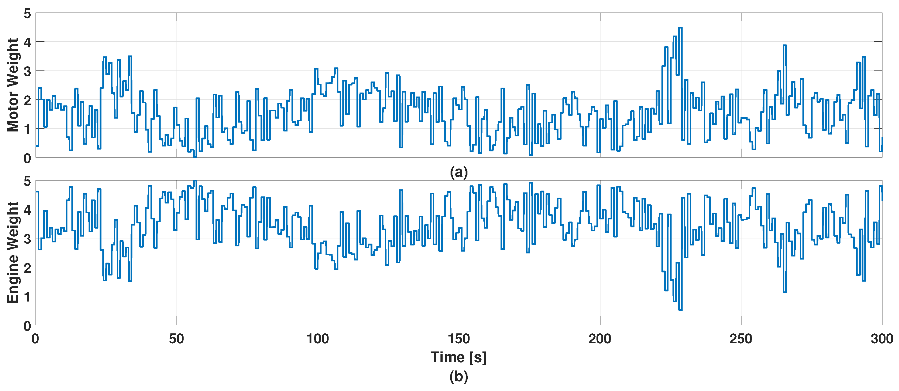
The main aim is to increase energy performance and decrease fuel consumption by modifying the weight terms. In this way, better optimization can be provided for the torque distribution problem.

For the DQN design, axle-based torques are predicted by using the forward-first four reference velocities, actual vehicle velocity, and resistance forces with the same principle in Equations (7) and (13); then, they are assigned as DQN states. The cost function consists of the internal combustion engine power, electric motor power, and associated battery power. The reason why the DQN states are chosen as mentioned is that DQN can establish a link between the predicted axle-level torque values and these power values.

In order to determine the weights of the cost function, the DQN action set is determined between 0.1 and 5. The weight coefficient used for the electric motor power W${}_{Mot}$ is determined during the training and transferred to MPC as an action value. The weight of the battery W${}_{Batt}$ is selected as W${}_{Mot}$ for the sake of simplicity. The weight coefficient of the internal combustion engine power W${}_{Eng}$ is chosen as the complement of the weight coefficient of the electric motor. In other words, W${}_{Eng}$ is equal to subtract the trained weight W${}_{Mot}$ from 5, which is the specified maximum weight. Two traction sources work in coordination. Using this relationship, the computational load and complexity of the training are reduced by training only the motor power’s weight instead of two weight terms. The DQN state and action for energy minimization via weight are given in Equation (56).

$$\begin{array}{cc}\hfill s_k& \hfill ={\displaystyle \frac{\left(\right|{\sum }_{j=0}^3{a}_{Ref}(k+j)-a_{Veh}\left(k\right)|m-F_{TotR})r}{N_{Gear}{N}_{FDR}}}\hfill \end{array}$$

(55)

$$\begin{array}{cc}\hfill a& \hfill =[0.1-5]\in R\hfill \end{array}$$

(56)

where a${}_{Ref}$ and a${}_{Veh}$ are the reference acceleration and vehicle acceleration, respectively. By using the reward function, the DQN agent learns to optimize the MPC weight terms to minimize the total power consumption of the system and to maximize the motor and engine efficiencies. The agent learns to select the torque distribution among the axles that results in the highest efficiencies while still meeting the performance requirements of the system.

The use of this reward function provides a strong incentive to the agent to improve the energy efficiency of the system. The reward function provides informative feedback to the agent on the energy efficiency of its behavior and guides the agent towards the optimal policy that maximizes the motor and engine efficiencies. In this direction, the reward function is given in Equation (57).

$$\begin{array}{c}{r}_k(s,a)=\left\{\begin{array}{cc}f(Mo{t}_{Eff},En{g}_{Eff}),\hfill & \mathrm{if}{\displaystyle \frac{Mo{t}_{Eff}+En{g}_{Eff}}{2}}>Li{m}_{Eff}\hfill \\ -f(Mo{t}_{Eff},En{g}_{Eff}),\hfill & \mathrm{otherwise}\hfill \end{array}\right.\hfill \end{array}$$

(57)

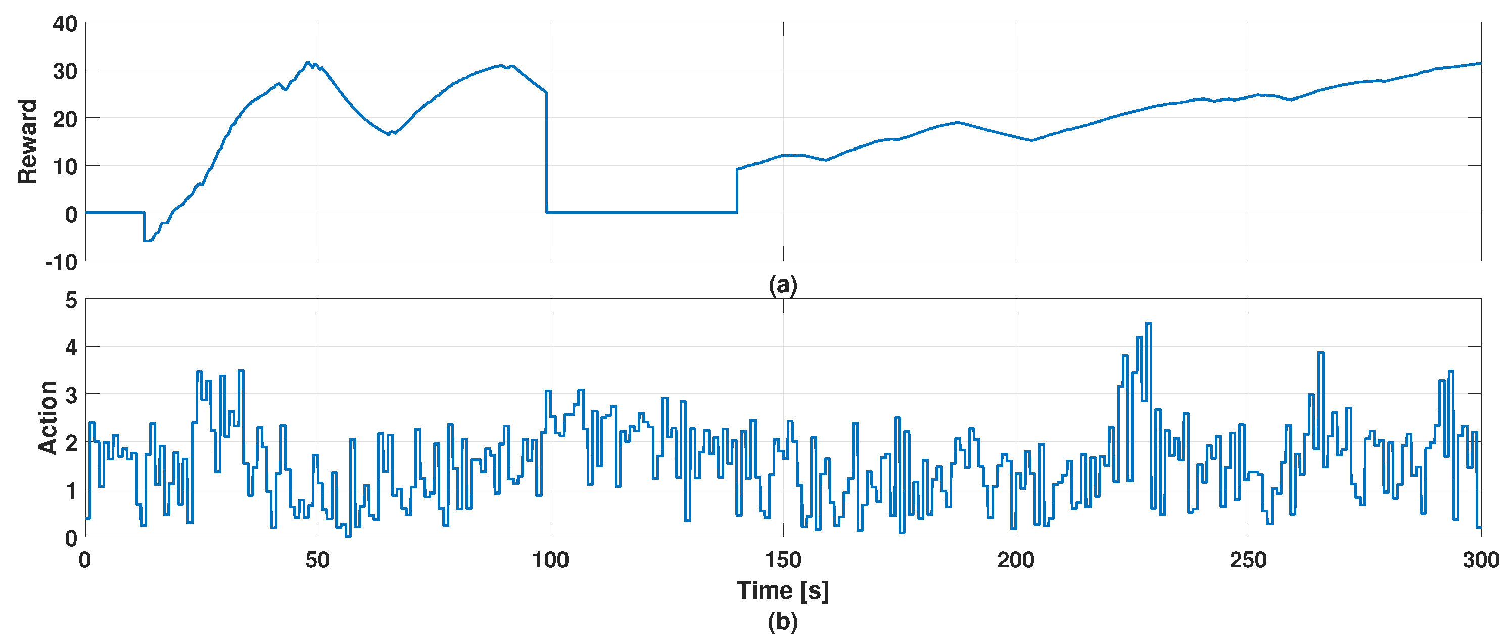
For the reward function that tries to maximize the average efficiency of the motor and engine, if the average efficiency is higher than the value of the limit parameter, which is Lim${}_{Eff}$, the difference is given as a reward via the 1D lookup table. If the average efficiency is lower than the value of the limit parameter, the difference is multiplied by the adjustment parameter and used as a punishment.

The same neural network structure of 3 hidden layers with 24 rectified neurons for each layer is used. For the training hyperparameters, the learning rate, discount factor, epsilon, and mini batch size are determined to be 0.001, 0.99, 0.95, and 64, respectively.

5. Results and Discussion

In this section, the first and second MPCs and vehicle outputs are demonstrated.

The first 300 s of the WLTP are used as a reference. The reason for using the first 300 s of the WLTP test cycle is that they are considered to be representative of typical urban driving conditions. During this phase, the vehicle undergoes multiple acceleration and deceleration cycles, simulating stop-and-go traffic and city driving. The results of the total torque demand of the first MPC, which is the total torque request control signal, and the torque distribution of the second MPC, taking into account the corresponding constraints of the engine and the motor, are given in Figure 10.

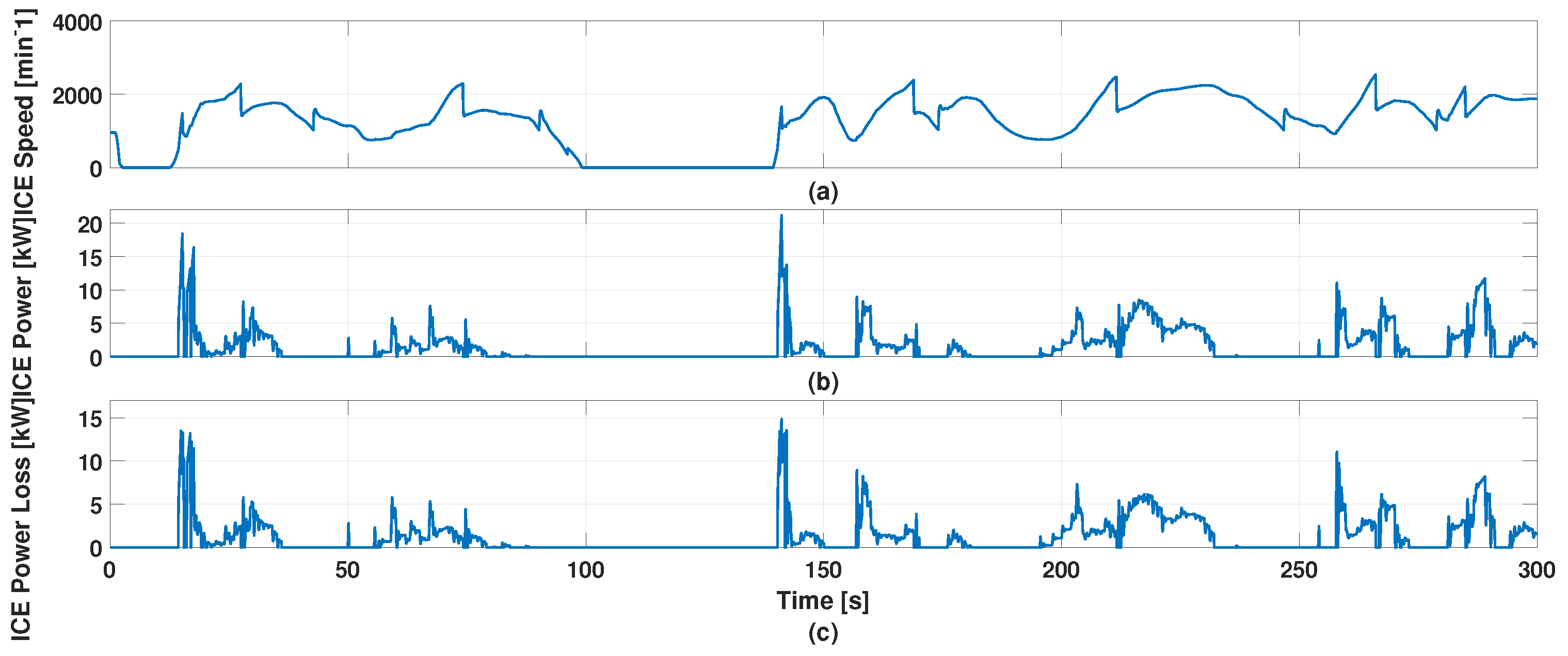
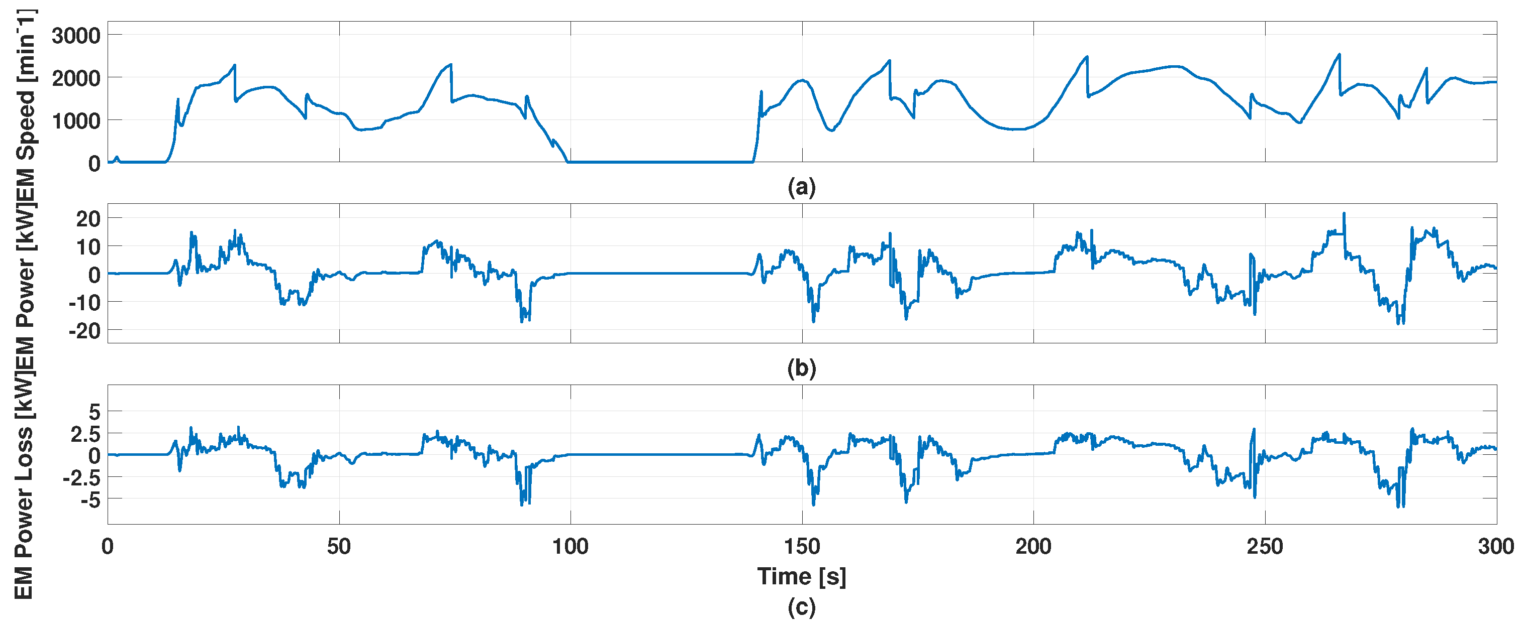
In Figure 11 and Figure 12, the torque produced by the engine and motor, shaft speed, consumed power, and lost power results are given.

The gear shifting of the gearbox is performed via the lookup table based on the accelerator pedal and vehicle velocity, which is converted from the output shaft speed. The gear shifting results, which are obtained by also considering the slope of the road, are given in Figure 13. For some period of the simulation, due to the braking priority, the accelerator pedal is set to zero.

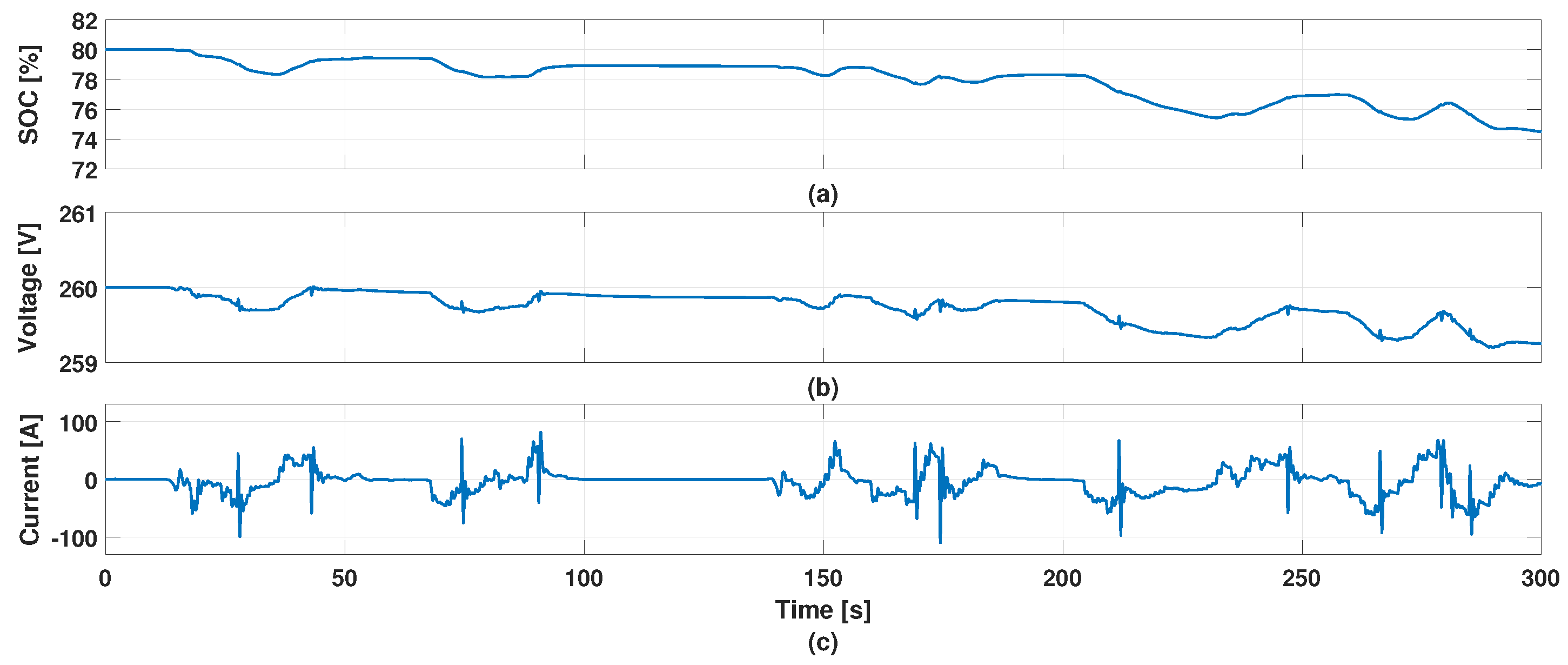
The SOC, voltage, and current results are given in Figure 14 for the battery. When the SOC is 80%, a voltage of 260 V is provided, and the voltage value changes as the SOC value changes. Other factors affecting the change in the voltage value are the ohmic resistance and the double-layer effect (Butler–Volmer). In line with these effects, relaxation is observed between 80 and 140s. The charging current is shown as a positive value, the discharging current is shown as a negative value, and it is observed that the current is between the limits, which are the MPC current constraints given in Figure 7.

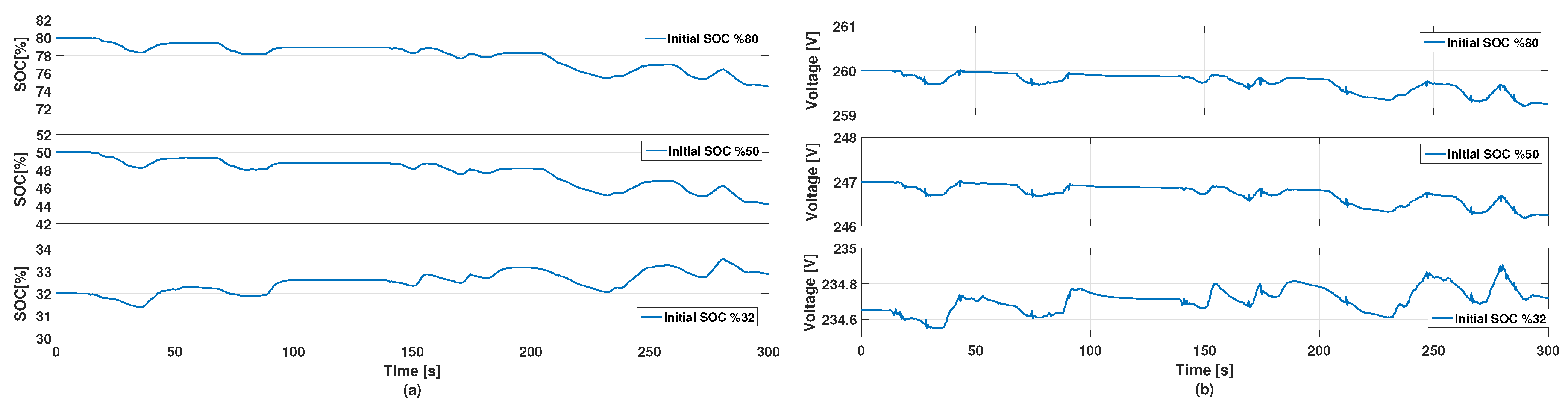
In order to examine the behavior of MPC with different initial SOC values and its results against the SOC constraint, simulation results are obtained by assigning an initial SOC value from the upper SOC limit, a value from the middle of the SOC limit, and a value close to the lower SOC limit. At different initial SOC values, it is observed that it does not violate the SOC constraints, and there are differences in the behavior of MPC. In order not to violate the SOC lower limit, it is observed that the electric motor generally works in the charging regions. While the initial SOC values are 80 and 50, it is observed that the electric motor is frequently used for higher efficiency. Additionally, the battery voltage values also change due to different initial SOC values. The SOC and battery voltage results are given in Figure 15.

In the simulation where the initial SOC value is close to the lower limit, the current values are usually in the positive (charging) region, not to violate the SOC lower limit. However, in the simulations with the initial SOC values of 80 and 50, a similar current profile with frequent charging and discharging is observed in Figure 16.

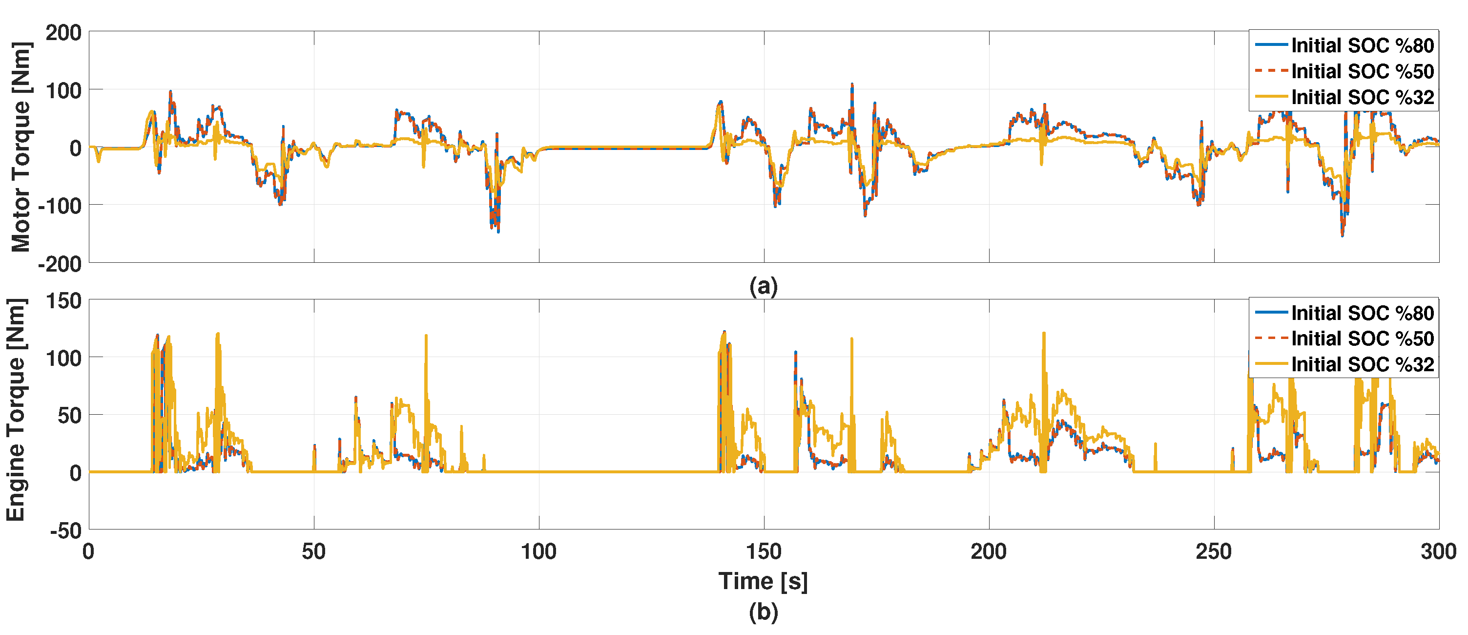
Finally, motor and engine torque behaviors are given at different initial SOC values in Figure 17. In the simulation, where the initial SOC value is close to the lower limit, the motor is generally used as a generator, and the engine mainly provides the requested traction torque.

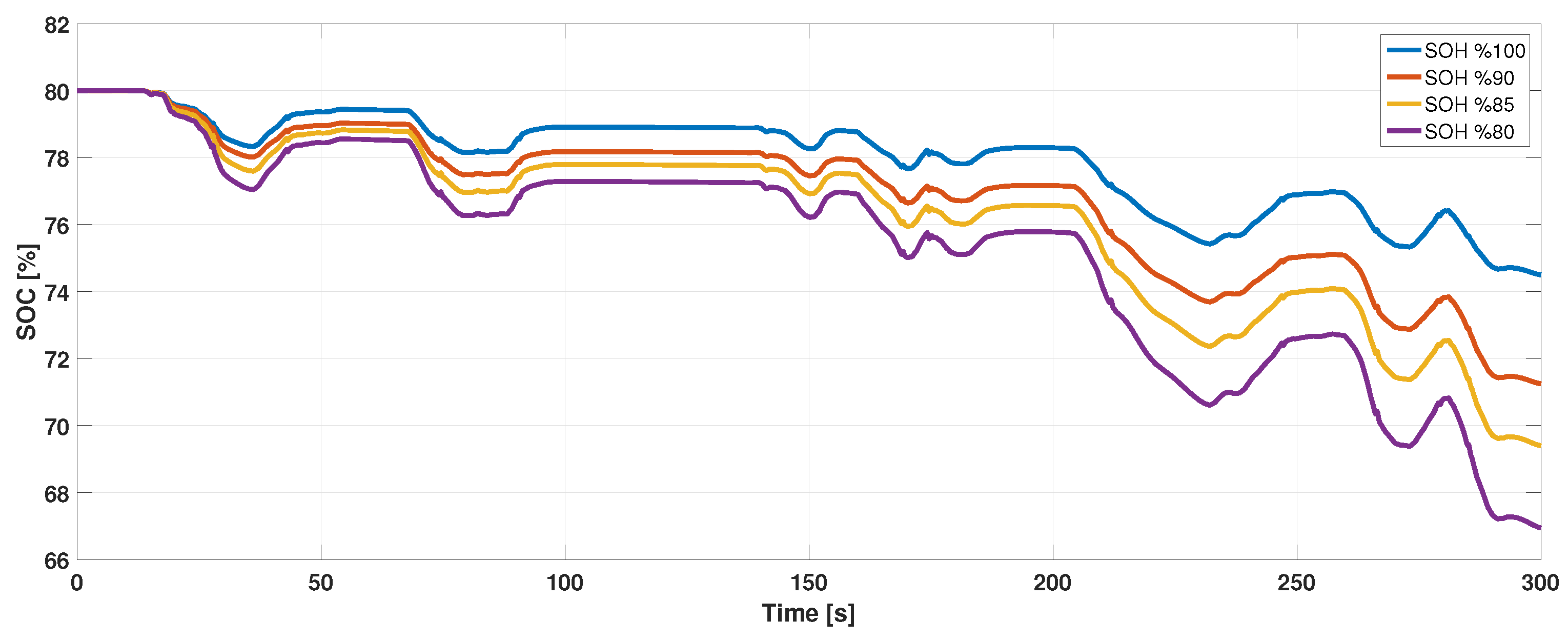
An examination of the effects of the SOH on the SOC is one of the important points of this study. The battery chemistry, cycle aging, and cell temperature are the main factors in SOH changes. The cycling aging and cell temperature effects on the SOH are shown in accordance with the SOC window in Figure 18.

In the figure above, the SOH effect of the battery under different conditions is examined. Under the conditions of 3200 cycles and a cell temperature of 25 °C, the SOH is 90%, the internal resistance is equal to 108.5% of the initial resistance value, and Q${}_{Max}$ is equal to 5.85 Ah. Under the conditions of 4400 cycles and a cell temperature of 25 °C, the SOH is 85%, the internal resistance is equal to 116.4% of the initial resistance value, and Q${}_{Max}$ is equal to 5.525 Ah. Under the conditions of 5500 cycles and a cell temperature of 25 °C, the SOH is 80%, the internal resistance is equal to 130.2% of the initial resistance value, and Q${}_{Max}$ is equal to 5.2 Ah.

When the figure is examined, the battery capacity decreases under these effects; when the SOC shows the same value, serious time differences occur, and it is observed that the battery discharges faster when the SOH is low.

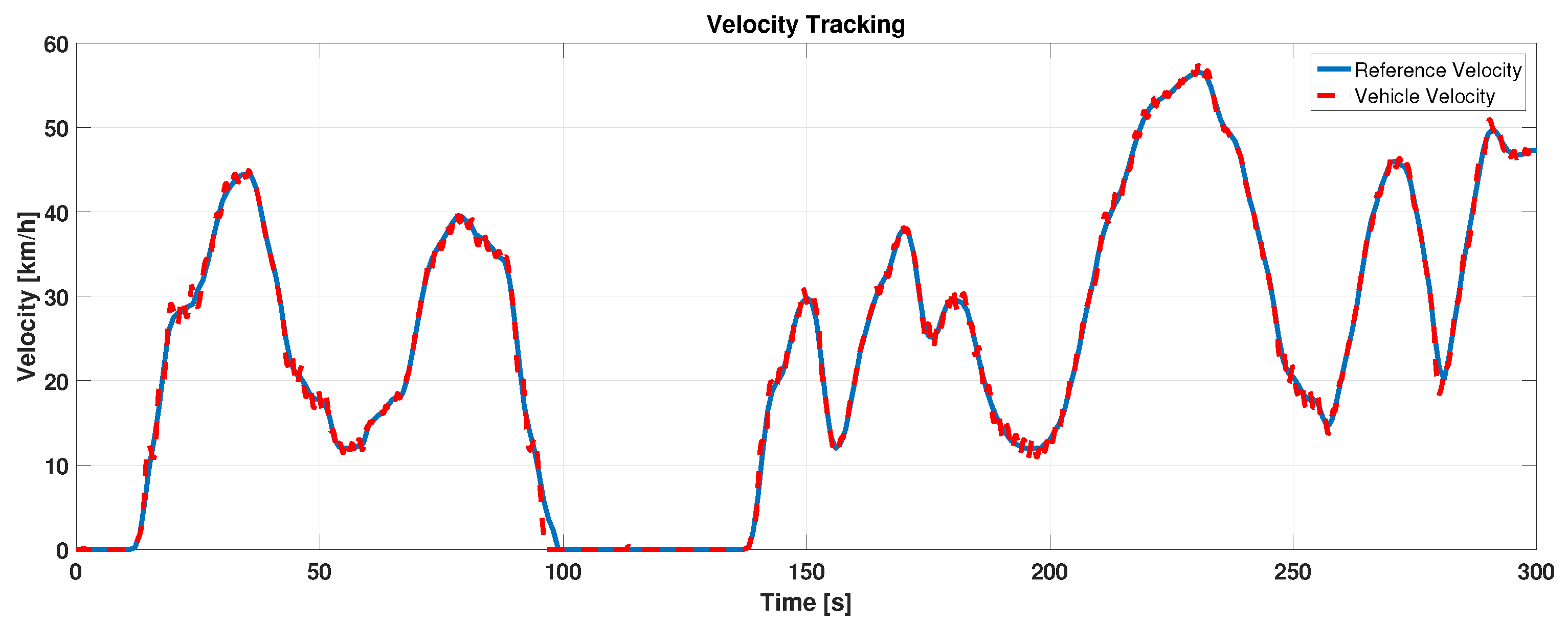
Finally, the velocity tracking results are given in Figure 19.

Event-triggered MPC with a DQN agent can achieve similar or better performance than traditional time-triggered MPC while reducing communication and computation requirements. For the event-triggered mechanism via DQN, the reward and action, which are designed based on the number of triggers and the error in velocity tracking, are given in Figure 20.

After observing that similar tracking velocity results are achieved with less triggers, it is aimed to reduce motor and engine losses by modifying the weights with DQN. To test the MPC whose weights are provided by DQN and to compare the performance with the previous method, which is without DQN, results are generated. For the WLTP reference, the motor and engine weights obtained with DQN are given in Figure 21, and the DQN reward and action are given in Figure 22.

For energy minimization in WLTP, the engine and motor operational points are marked and plotted on efficiency maps. The cyan marks represent the method without DQN, and the white marks represent the DQN weight algorithm as in Figure 23 and Figure 24.

Indicating energy savings and fuel consumption figures via algorithms with and without DQN can be important for providing a way to quantify and compare the performance of different control strategies and algorithms for improving energy efficiency in vehicles. This is why the fuel consumption results are given in Figure 25. The Simulink Simscape engine module allows us to model and simulate the behavior of an engine. Additionally, it provides the power output of the engine under different operating conditions. However, brake specific fuel consumption (BSFC), which is obtained from the given vehicle specifications, is a measure of the amount of fuel consumed by an engine per unit of power produced and provided by the Simscape model. Then, it is converted to the fuel consumption in units of g/s for comparison purposes. As shown in Figure 25b, the event-triggered double-MPC structure with DQNs performs the drive cycle under consideration with less fuel consumption in terms of gram per second. In addition, the total consumption is derived as 102.076 g with the event-triggered double-MPC structure with DQNs, while it is calculated as 104.996 g with the classic double-MPC structure by integrating fuel consumption.

After the triggering instances and weight training, the execution time, triggering number, average velocity error, and motor and engine efficiency values are as shown in

Table 10. Efficiency Results in WLTP.

Criteria	Structure with Two MPCs Connected in Series	Structure with Two Event-Triggered MPCs with DQNs Connected in Series
Triggering Number	30,000	14,396
Execution Time (s)	13.881 s	7.815 s
Engine Efficiency (%)	19.26%	22.12%
Motor Efficiency (%)	78.95%	82.56%
Average Velocity Error Per Sample (km/h)	0.0342 km/h	0.0518 km/h

for the WLTP reference.

The purpose of the event-triggered mechanism is to reduce the computational cost by triggering the controller less frequently. It aims to follow the velocity reference as much as possible while reducing the computational cost. The execution time of a simulation depends on various factors, such as the complexity of the system being simulated, the accuracy and resolution of the simulation model, the computational resources available, and the simulation software being used. Overall, using multiple measurements of execution time can help to reduce the impact of instant factors on the results, improving the accuracy and reliability of the measurements. This is why the execution time is measured more than ten times, and the average execution time is used as a result via the Simulink Profiler Toolbox.

As can be seen in

Table 11. Simulink Profiler Report.

Criteria	Time (s)	Calls	Time/Calls	Self-Time (s)
Structure with Two MPCs Connected in Series	15.321 s	30,000	0.0005107	13.881 s
Structure with Two Event-Triggered MPCs with DQNs Connected in Series	8.982 s	14,396	0.0005087	7.815 s

, the classic double-MPC structure and event-triggered double-MPC structure are compared. In a Simulink Profiler report, time refers to the total execution time of the subsystem, including the time spent executing its own code, as well as any code in the MPC subsystem. Self-time, however, only refers to the time spent executing the code directly within the MPC, without including any time spent executing the code in its elements, which transfer the outputs. Calls indicate the event-triggered number, and the time/call metric refers to the average execution time of MPCs per function call. The results represent the performance of two MPCs in total. According to the results, the event-triggered mechanism reduces the execution time by triggering fewer controllers.

After this stage, the weights of MPC are trained with DQN to distribute the torque more efficiently. According to the results, the efficiency of the motor increases by 3.61%, while the efficiency of the engine increases by 2.86%. This efficiency increase is achieved by triggering 52.01% fewer controllers. Thus, while the computational cost is reduced, the energy efficiency is also increased with MPC and DQN.

6. Conclusions

In this study, the energy management problem for HEVs is studied. HEVs have different types with different architectures; a Kia Niro with the P2 HEV configuration is modeled in this study. Since there are limited data about the battery pack in the publicly shared vehicle information, the appropriate battery and cell are selected for the vehicle, and vehicle modeling is detailed. The first MPC is designed to follow the WLTP velocity reference. The first MPC calculates the total torque that must be requested in accordance with the comfort–acceleration limits for velocity reference tracking. With the second MPC, this total demanded torque value is distributed between the motor and the engine. During torque distribution, the physical limits of the motor and engine are taken into account. In addition to the motor and engine, the battery also has physical limitations. These constraints are that the SOC operates within a certain range and current limits, and SOH effects are also taken into account in the second MPC. In traditional MPCs, the control action is computed at every sampling time based on the current system state and a prediction of future system behavior. In an event-triggered MPC approach, the control action is only computed when certain triggering conditions are met, such as when the system behavior deviates from a predefined threshold or when a specific event occurs. This approach can reduce the computational burden of MPC while maintaining the control performance, making it suitable for systems with limited computing resources or applications where frequent updates of the control action are not required. An event-triggered mechanism is designed with DQN to reduce the computational cost. Finally, the weights of the second MPC are trained with DQN to increase efficiency. The efficiency of the motor increases by 3.61%, while the efficiency of the engine increases by 2.86%. Moreover, the efficiency increases of the motor and the engine are realized with 52.01% less triggering. We aim to show that MPC performance can be increased using methods such as DQN in the energy management problem. With this proposal, an efficient energy management strategy is provided with less computational cost.