Data Driven Methods for Finding Coefficients of Aerodynamic Drag and Rolling Resistance of Electric Vehicles

Abstract

This research investigated an alternate method for establishing the complex coefficients used in an electric vehicle’s mathematical energy consumption model. While other methods for creating electric vehicle energy models exist, it would be beneficial to have a rapid and inexpensive technique that remains accurate. Producing a mathematical energy model for such a vehicle has the challenge of determining its aerodynamic drag and rolling resistance coefficients. Currently and most often, expensive and tedious (time-consuming) methods are used to find these coefficients. Computational fluid dynamics (CFD), wind tunnel testing, and extensive mathematics make this objective challenging. For this work, a solar-powered electric vehicle provided the source data to derive its coefficients cost-effectively and efficiently. Data were collected during a road test of the solar electric vehicle from South Africa to Namibia stretching over 2000 km, in which all required energy variables were recorded. The collected data were used in an optimisation routine to establish the two coefficients by minimising the actual and modelled energy consumption error and controlling the driving speed. The outcome of the optimisation routine produced accurate coefficients with a final error value of less than 5% when applied to a validation data set not used during optimisation. With minor modifications, this method may be integrated into any electric vehicle computer system to autonomously identify its two hard-to-find coefficients while driving, which can be used to provide an accurate and realistic driving range estimation to the driver.

1. Introduction

1.1. Context

There is a global trend toward moving away from using internal combustion engine (ICE) vehicles in favour of electric vehicles (EVs). This trend has become evident in the development of an entirely new market that aims to provide an alternative mode of transport that does not use hydrocarbons while driving. This development has come about in tandem with the effects of climate change on the environment. Rapid advances in technology and complex data analysis are also facilitating the trend.

The European Union aims to ban the sale of all ICE vehicles by 2035 to meet the low-emission objectives set out in the European Green Deal [1,2]. To this end, the European Green Deal has stipulated the upper limits for global temperature increases going forward [3]. In the transportation sector, the emergence of EVs is the most prominent indicator of development trends toward achieving these objectives.

This research seeks to increase our understanding of the EV further. This study was conducted using a solar electric vehicle (SEV), as it was the medium available to provide the source data for the analysis. The fact that solar panels were used on the vehicle was not relevant to this particular research. SEVs originate from the same concept as standard EVs, except that in SEVS, the sun can also charge the battery rather than only conventional charging methods (plug-in points).

The top surface of an SEV is covered with solar panels that supply energy to the vehicle’s battery. Its developers also had to incorporate a design element to optimise its aerodynamic efficiencies, resulting in the smallest possible frontal area. In implementing these features, an unusual design shape emerged.

The SEV that was analysed for this study was built by a team at the Tshwane University of Technology (TUT) from 2020 to 2021. The final product can be seen in Figure 1.

SEVs must be optimised in every way possible to maximise their travel distance. A major inhibitor against the general public’s acceptance of any electric vehicle is a concept termed ‘range anxiety’ [4]. Range anxiety is anxiety attributed to the inaccuracy of estimating the remaining travel range in an EV. Unlike an ICE vehicle, an EV needs time to charge. With current charging technology, this process is more time consuming than filling a vehicle with fuel. Therefore, taking a trip with an EV requires planning. This issue can only be confronted by accurately predicting how far an EV can travel before recharging. For this, a precise energy model of the vehicle is required.

When creating a vehicle model, most factors influencing the model can easily be calculated or measured, except for two variables. These are the coefficients of aerodynamic drag (C_d) and rolling resistance (C_r). The coefficient of aerodynamic drag is typically found using computational fluid dynamics (with expensive software licences) or wind tunnel testing, and the coefficient of rolling resistance is found using tedious testing and complex mathematics. This study aims to find an alternate and effective way to determine the coefficients required to model a vehicle’s energy consumption.

There are various ways of mathematically modelling vehicles, but there is always a need to improve these methods for better results. The creation of a more straightforward and rapid method for modelling an EV demonstrates its significance and is the focus of this research.

1.2. Literature Review

Significant SEV development in South Africa began when a national solar car challenge was introduced in 2012. The Sasol Solar Challenge (SSC) is a biennial event where teams from around the world come to South Africa to compete using custom-built solar cars [5]. The event is termed a “challenge” and not a “race”, as the participants’ objective is to cover the most distance rather than travel with the most speed. As a result of this event, multiple SEVs were developed by TUT. Their third- and fourth-generation cars won first place amongst the South African teams in the last two events.

Their fourth-generation SEV was subjected to substantial testing in the lead-up to the 2022 SSC. This included driving the vehicle over 2000 km on solar power alone from Pretoria, South Africa, to Swakopmund, Namibia. The road test took place over seven days, with predetermined routes and stopping points set for each day. Comprehensive data, such as mechanical, electrical, and environmental parameters, were recorded during the solar car’s drive to Namibia, and these data will be used for the study.

The route map can be seen in Figure 2. The endpoints of each day were the two South African towns of Vryburg and Upington, and the rest were the towns of Grunau, Keetmanshoop, Mariental, Windhoek, and Swakopmund in Namibia.

1.2.1. Mathematical Modelling of Vehicles

The modelling of a vehicle is a concept that has been around for several years [6,7]. These models are often used in the field of EVs, as it is necessary to predict how far a vehicle can travel given certain driving conditions. While a vehicle is moving, it is subjected to different forces. The analysis of these forces is essential for understanding a vehicle’s behaviour thoroughly. An understanding of its behaviour enables a vehicle to be mathematically modelled [8].

Vehicles can be modelled for various applications, such as identifying the individual components of EVs, the effects of EVs on the environment, or EV patterns for travel planning [6,9,10,11]. This research focused on creating an accurate mathematical energy consumption model of an EV to analyse its performance.

Significant research has been conducted for the creation of mathematical models of vehicles [6,7,8,9,12,13]. This process generally starts by examining the forces that act on such a vehicle. The most prominent of these have been shown to be the drag force ($F_d$), the rolling resistance force ($F_r$) and the force due to gravity ($F_g$) [6,12,13]. These forces can be quantified and calculated using the following formulas:

$$F_d=\frac{1}{2}\rho A{C}_d{\left(v+v_w\right)}^2$$

(1)

$$F_r=C_{r}mg\cos \left(\theta \right)$$

(2)

$$F_g=mg\sin \left(\theta \right),$$

(3)

where $\rho$ is the air density, $A$ is the frontal area of the vehicle, $C_d$ is the coefficient of aerodynamic drag, $v$ is the velocity of the vehicle, $v_w$ is the velocity of the wind relative to the heading of the vehicle, $C_r$ is the coefficient of rolling resistance, $m$ is the mass of the vehicle and driver, $g$ is the acceleration due to gravity, and $\theta$ is the angle of the road (incline or decline). Other, more significant, auxiliary energy consumption factors include the force due to acceleration and the power usage of the vehicle’s onboard electronics, but these are not included in this study because they had a minimal impact on the overall system.

1.2.2. Optimisation

Mathematical optimisation aims to create the best possible result of a problem by determining the maximum or minimum solution for an objective function while examining and varying specific parameters that affect the problem [14].

Having the optimal values for each parameter of a model produces the best overall model. For Equations (1)–(3), the optimal values for air density, the frontal area of the vehicle, the velocity of the vehicle, the velocity of the wind, the vehicle mass, the acceleration due to gravity, and theta can be easily found because they are measured, calculated, or known constants. The aerodynamic drag and rolling resistance coefficients are more difficult to obtain [15,16]. This research aims to optimise these two coefficients by minimising the error between the real and modelled energy consumption profiles of the data collected during the trip from South Africa to Namibia.

A standard method for finding these two coefficients is to use coast-down tests [15,16,17]. These tests are challenging to implement as perfect conditions rarely occur. For example, the roads need to be flat (perfectly horizontal), and there should not be any wind nor fluctuation in air density. Coast-down tests seek to find both coefficients simultaneously by measuring the total driving resistance of a vehicle. It also involves measuring the vehicle’s velocity and time it takes for it to coast to a stop from a certain maximum velocity [18]. Distinguishing between C_d and C_r forces from data obtained using such a method is approximate and, therefore, not as accurate as it could be.

The optimisation process for this work will be performed using MATLAB, or more specifically, the MATLAB fmincon function [19]. This function can make use of interior-point, trust-region reflective, sequential quadratic programming (SQP) and active-set optimisation algorithms. This research will make use of SQP as the optimisation solver.

SQP is a mathematical method used for finding solutions to non-linear optimisation problems made up of quadratic functions (such as those required in this research) [20]. This, along with the fact that SQP is a ‘medium-scale’ algorithm, means that the optimisation problem can be solved quickly while still satisfying the chosen constraints on every iteration of the routine [19,21]. This is important as the constraints set up in this research play a significant role in creating accurate results. The advantage of the SQP algorithm is that the computational time for this specific problem was much faster than that of the others mentioned above.

An optimisation problem can be set up using an objective function [20,22]:

$$\underset{x}{\mathrm{minimise}} f\left(x\right)$$

(4)

and also by including applicable constraints [20,22]:

$$\begin{array}{c}g{\left(y\right)}^{min}\le y\le g{\left(y\right)}^{max}\\ h{\left(z\right)}^{min}\le z\le h{\left(z\right)}^{max}.\end{array}$$

(5)

These principles can be applied to recorded data to derive values for C_d and C_r, which are needed for modelling vehicles. This research is necessary, as an accurate and more straightforward method will be beneficial for determining these coefficients. MATLAB establishes proof of the concept for this research. However, the programming can be performed using open-source software to reduce the cost of finding these coefficients.

1.2.3. Existing Noteworthy Research

Some interesting research has been conducted on analysing EV energy performance in the last decade. The focus has specifically been placed on increasing the driving range of an EV. Mruzek et al. [23] identified a vehicle’s weight, motor size, and aerodynamic drag coefficients as key factors that affect the performance of an EV. The authors concluded that vehicle weight is attributed to the biggest loss of energy, but driving style also plays a significant role [23]. Szumska and Jurecki [24] stated that the range a vehicle can travel directly correlates with the vehicle design, the driving style of the vehicle operator, and the conditions surrounding the vehicle. Vehicle design incorporates the coefficients of aerodynamic drag and rolling resistance [25].

Kiyakli and Solmaz [25] mentioned that force due to aerodynamic drag, force due to tyre rolling resistance, and force due to gradient resistance (Equations (1)–(3)) are all important parameters concerning a vehicle’s energy consumption. The research further states that force due to aerodynamic drag is one of the most significant factors when considering energy loss, with a vehicle’s velocity and aerodynamic drag coefficient significantly altering this force [25]. Its velocity plays a prominent role, as it is exponential alongside an increasing speed, as seen in Equation (1). Another large factor that influences the energy consumption of a vehicle is its force of rolling resistance [26]. This force is complicated to calculate, as the coefficient of rolling resistance is challenging to measure. Ejsmont and Owczarzak [26] mentioned that this is the case because there are many factors that can affect this coefficient, such as the different road surfaces and temperatures experienced by tyres.

Another factor that affects the energy consumption of an EV and is very sensitive in achieving accurate results is the vehicle’s motor efficiency [27]. The research found that an efficiency map comparing the torque and revolutions per minute of a motor plays a significant role in obtaining precise results [27]. Mavlonov et al. [27] compared three different motors to compare the sensitivities of their efficiency maps based on the different efficiency characteristics. Their research discovered that the motor size (power) and efficiency map are the main factors that influence energy consumption. Asamer et al. [28] analysed multiple factors that influenced the model of a vehicle and arrived at a similar conclusion. The researchers discovered that the overall efficiency of a vehicle is the biggest parameter affecting its energy loss and is mainly attributed to the efficiency of the motor [28]. This conclusion was determined by analysing the sensitivity of the energy demand in electric vehicles.

The literature reviewed shows that the aerodynamic drag, rolling resistance, and efficiency of the motor affect a vehicle’s energy consumption significantly. This work is, therefore, important, as it provides a more straightforward method for finding the coefficients of aerodynamic drag and rolling resistance, which can assist others with their energy management strategies.

2. Materials and Methods

Figure 3 below shows an overview of the methodology used in this work, followed by an in-depth, detailed explanation of each step of the process.

Phase 1: Literature review.

Firstly, the literature was consulted to develop an understanding of what research has been performed in the area of study as well as what knowledge gaps there are in this field. This review of the literature was also used to gather the information required to perform the tasks to solve the research question.

Phase 2: Data collection.

This work required a substantial amount of data to be collected to determine the parameters that accurately depict the vehicle’s behaviour. These data were collected from sensors placed around the SEV. The data were managed and stored using microcontrollers.

Phase 3: Data pre-processing.

The collected data was then imported into MATLAB so that it could be pre-processed. This involved joining the data collected from different sources and creating a useable data set for the next phase of research.

Phase 4: Analytical modelling.

A mathematical energy consumption model of the SEV was then developed. This was used to create an understanding of how much energy the SEV used on each day of the trip. All parameters for this model were known except for the coefficients of aerodynamic drag and rolling resistance.

Phase 5: Optimisation.

The real energy used by the SEV (i.e., the collected data) could then be compared against the modelled energy of the SEV. As the two coefficients from the model were unknown, the error between the two energy comparison profiles was minimised to arrive at values for the coefficients.

Phase 6: Validation and performance analysis.

The newly found values for these coefficients were then inserted into the model to validate if they were realistic. The percentage error between the real and modelled energies after validation was used to confirm how realistic the coefficients were.

2.1. Data Collection

The data used in this study were collected from two sources and stored in .csv format using local data logging equipment. The first part of the data was from the SEV, and the second part was from a compact weather station placed on top of a support vehicle (SV). The MaxiMet GMX501 weather station, developed by Gill Instruments, was used. The SV was the command centre where all live telemetry data received from both the SEV and weather station were visualised and analysed for better energy planning during the trip. These observations were performed to monitor the SEV and collect data from both the SEV and weather station for use in making predictions, such as the desired speed for maximising the travel distance of the SEV. Figure 1b shows the SEV in the foreground and the SV in the background with the weather station attached. The weather station was placed as high up as possible to avoid unwanted aerodynamic disturbances.

The required parameters recorded from the weather station can be found in

Table 1. Data that was collected from the weather station.

Parameter	SI Unit	Point of Collection
Air density	(kg/m3)	Calculated
SV velocity	km/h	Measured
GPS elevation	m	Measured
GPS heading	Degrees	Measured
GPS latitude	Degrees	Measured
GPS longitude	Degrees	Measured
Humidity	%	Measured
Incline of the road	Degrees	Calculated
Pressure	Pa	Measured
Temperature	°C	Measured
Time	h:m:s	Measured
Wind direction	Degrees	Measured
Wind velocity	km/h	Measured

. Table 1 also states whether the parameter was measured using an actual sensor or calculated from the data of multiple sensors.

The other recorded parameters were stored on the SEV. The battery voltage of the vehicle was monitored at a frequency of 3 Hz, as obtained from the battery management system (BMS). Its electrical current was measured using a current sensor installed between the vehicle’s motor and its motor controller. In doing so, only the electrical current consumed by the motor was measured (isolating the traction circuit power usage). The placement of the electrical current sensor meant that the input from the solar panels and usage of onboard electronics was disregarded. This can be seen in Figure 4.

These variables are not important for this research, as our concern is only on the power used by the traction circuit of the vehicle. Its tractive power was calculated using these electrical current and voltage readings. A timestamp was also recorded for every interval of data collected. Using these data, it is possible to calculate the energy consumed or re-generated by the motor of the SEV.

The recorded parameters collected from the SEV’s systems can be seen in

Table 2. Data that was collected from the SEV sensors.

Parameter	SI Unit	Point of Collection
Battery voltage	V	Measured
Motor current	A	Measured
Motor energy	kWh	Calculated
Power	W	Calculated
Time	h:m:s	Measured
SEV velocity	km/h	Measured

.

2.2. Data Pre-Processing

The first step in pre-processing the data was to join the two data sets from the two separate sources. Care was taken because the two sources were recorded by their respective sensors at different frequencies. The weather station data were recorded at 1 Hz, and the data from the onboard SEV sensors were recorded at 3 Hz. The recording frequencies for the two data sources were adequate for the expected rate of change of the variables observed. Averaging methods were used to rework the 3 Hz data down to 1 Hz with the assistance of a timestamp to ensure the data were synchronised. The time synchronisation of the data was of the utmost importance. The joint sources created the final data set.

The next important step was to determine what data should be extracted from the final data set to use for this research, as the SEV was not always moving during each day of the trip. It would occasionally be stopped for reasons such as alternating the driver of the vehicle, routine inspections, or repairs. This stop time is not helpful data and was, therefore, omitted from the analysis. The stop times marked points for splitting each day of driving into sessions. These sessions were then concatenated again to form a day’s worth of driving data (containing no zero-speed data).

Each day of pre-processed data could then be joined with other days to form a larger data set for analysis to represent the system better. The more useable data there is that can be compiled together, the more comprehensive and realistic the depiction of that data is.

A percentage of the data could then be used to determine the C_d and C_r values using the optimisation algorithm (data used for optimisation). The remaining data could then be used to validate the coefficients found to determine the accuracy of the process (data used for validation).

Table 3. Summary of driving conditions.

Day	Town Start	Town End	Road Type	Distance (km)	Velocity (km/h) 1	Energy Consumed (kWh) 2
1	Pretoria, SA	Vryburg, SA	Flat	406	-	-
2	Vryburg, SA	Upington, SA	Descent	394	66	3.75
3	Upington, SA	Grunau, NM	Ascent	182	68	1.93
4	Grunau, NM	Keetmanshoop, NM	Hilly	155	66	1.47
5	Keetmanshoop, NM	Mariental, NM	Hilly	236	74	2.61
6	Mariental, NM	Windhoek, NM	Ascent	268	64	3.03
7	Windhoek, NM	Swakopmund, NM	Descent	434	65	2.78

¹ Average. ² Battery energy consumed.

shows a summary of the driving conditions for each day.

Table 3 displays the start and end towns of each day of the trip, the overall road type for that day, the distance covered by the SEV, its average velocity, and how much battery energy was consumed by the SEV traction circuit during the day. This does not include the energy added or used in the collection of energy from the solar panels on the vehicle, nor does it include auxiliary component energy usage. Unfortunately, as a result of issues with the controller area network (CAN) bus, not all data were collected from the SEV on Day 1. This means that the data from Day 1 was omitted from this research.

Table 4. Summary of environmental conditions.

Day	Temperature (°C) 1	Air Density (kg/m3) 1	Humidity (%) 1	Wind Speed (km/h) 2	Elevation (m) 3
1	16–34	0.993–1.045	28–74	6, (137)	1374–1187
2	25–35	0.995–1.041	22–53	8, (128)	1210–820
3	28–36	1.006–1.065	22–49	7, (30)	811–1110
4	24–34	0.992–1.041	26–46	10, (45)	1110–935
5	25–33	1.010–1.057	32–41	10, (28)	935–1105
6	23–30	0.936–1.036	38–79	10, (44)	1109–1705
7	20–27	0.984–1.194	50–80	15, (102)	1698–21

¹ Minimum to maximum. ² Average, (gusts). ³ Start of day to end of day.

shows a summary of the environmental conditions for each day.

Table 4 displays the temperature, air density, and humidity throughout each day. It also shows the recorded wind speed. This wind speed can be used to determine how much of an effect the wind had on the drag force of the vehicle. Changes in elevation can also be seen. The elevation data show that the trip started in central South Africa at the highest point and ended at sea level in Namibia.

2.3. Modelling

To create an accurate mathematical model of a vehicle and to analyse its energy consumption performance, the components that make up the model need to be as precise as possible. These components can be seen in Equations (1)–(3). Each variable is either a constant or can easily be measured or calculated, except for the coefficients of aerodynamic drag and rolling resistance [15,16]. The measured or calculated variables can be seen in Table 1 and Table 2. There are no pre-defined values for these parameters, as they are dynamic. Equations (1)–(3) also have constant variables. The constant values and SI units can be seen in

Table 5. List of constants required for force formulas.

Parameter	Value	SI Unit
Frontal area of SEV	0.8	m2
SEV mass	200	kg
Driver 1 mass	80	kg
Driver 2 mass	63	kg
Acceleration due to gravity	9.81	m/s2
Wheel diameter	0.567	m
Specific gas constant (dry air)	287.058	J/kg·K
Motor efficiency constant	80	%

.

Using all of this information, an analytical mathematical model of the vehicle could be created using Newton’s second law [12,13]:

$$F_{net}=F_d+F_r+F_g$$

(6)

The model was created by comparing the force applied to move the vehicle forward (mass multiplied by acceleration) with the forces opposing motion (force due to drag, force due to rolling resistance, and force due to gravity).

For this research, the law of conservation of energy was used to compare the real and modelled energy used by the vehicle. Using the forces shown in Equation (6), the total loss of modelled mechanical traction power ($P_{loss}$) could be determined according to the model:

$$P_{loss}\left(t\right)=\left[F_d\left(t\right)+F_r\left(t\right)+F_g\left(t\right)\right]v\left(t\right)$$

(7)

The loss of modelled mechanical traction energy ($E_{model}$) could be calculated by integrating the loss of modelled mechanical traction power with respect to time:

$$\begin{array}{ll}{E}_{model}\left(t\right)={{\displaystyle \int }}_{t_i}^{t_f}& P_{loss}\left(t\right)dt={{\displaystyle \int }}_{t_i}^{t_f}F\left(t\right)v\left(t\right)dt\\ & =\frac{1}{\eta }{{\displaystyle \int }}_{t_i}^{t_f}(\frac{1}{2}\rho A{C}_d{\left(v\left(t\right)+v_w\left(t\right)\right)}^2+C_{r}mgcos\left(\theta \left(t\right)\right)\\ & +mgsin\left(\theta \left(t\right)\right))v\left(t\right)dt\end{array}$$

(8)

Equation (8) displays the modelled mechanical traction energy loss of the vehicle, where $t_i$ and $t_f$ are the initial and final times of the section to be analysed. The range of $t_i$ to $t_f$ is the length of the data collected in step sizes of seconds ($t$). The data were analysed in 1 Hz intervals.

The real (or measured) mechanical traction power available ($P_{real}$) to the system was determined using the battery voltage ($V)$ and the motor current ($I)$. This real mechanical power was calculated from the formula below:

$$P_{real}\left(t\right)=\eta \left(V\left(t\right)\times I\left(t\right)\right)$$

(9)

where $\eta$ is the electrical to mechanical conversion efficiency of the traction motor. The loss of real mechanical traction energy ($E_{real}$) could be calculated by integrating the real mechanical power with respect to time:

$$E_{real}\left(t\right)={\int }_{t_i}^{t_f}{P}_{real}\left(t\right)dt$$

(10)

The modelled mechanical energy that was predicted to be used could then be compared against the real mechanical energy actually used by the vehicle.

2.4. Optimisation

The basis of this research encompasses optimising (minimising) the root mean square error (RMSE) between the modelled energy used by the vehicle and the real energy used by the vehicle. The RMSE was used to quantify the error in this work. This process provided optimal values for C_d and C_r that could be used in Equations (1) and (2).

The cumulative real tractive power (Watt, obtained from Equation (9)) was measured every second to obtain the real energy used (Wh, calculated from Equation (10)) over a day (or recorded data session). An example of these data for Day 2 (between Vryburg, SA, and Upington, SA) can be seen in Figure 5a.

The blue curve displays the real energy used throughout the day, measured in seconds (Figure 5a). The red curve is the predicted energy used, which was calculated using a model that had pre-selected values for C_d and C_r to produce Figure 5a. The aim was to calculate these C_d and C_r values by minimising the error between the blue (real energy) and the red (modelled energy) data lines. An RMSE confidence bound can also be seen in Figure 5a. This confidence interval can provide a user with the statistical mean forecasted risk quantification. This may be useful to users when making energy decisions regarding the model output with the expected associated risk.

Figure 5b displays an example of the real and modelled power used by the vehicle over a short period on Day 2. Only a short period of data are displayed so that it is possible to see the difference between the two curves, as they follow each other very closely. The real power displayed seems to have jitter, which is possible as a result of output sensitivity in the throttle pedal sensor.

Table 6. Typical coefficients of aerodynamic drag with frontal area of vehicle types.

Vehicle Type	A (m2)	Cd
TUT 2nd generation SEV	1.27	0.23
TUT 3rd generation SEV	1.03	0.16
TUT 4th generation SEV	0.8	0.13
Aurora (2007)	0.76	0.1
Toyota Corolla (typical passenger vehicle)	-	0.27
Tesla Model S (electric passenger vehicle)	2.34	0.208
Tesla Model X (electric SUV)	2.59	0.24
Toyota Land Cruiser (4WD)	-	0.35
Truck (Heavy duty)	~3	~0.6

contains some typical aerodynamic drag coefficients (C_d value examples) with the frontal areas of different vehicle types to serve as a reference [29,30,31,32,33].

These vehicle types include the TUT second-, third-, and fourth-generation SEVs. The coefficients of the second- and third-generation solar cars were determined using CFD and wind tunnel experiments [22,34], and the C_d value of the fourth-generation solar car (Sunchaser 4) was recently announced [35]. The Aurora Vehicle Association (headquartered in Melbourne, Australia) began developing solar cars in 1987 [33]. The drag and rolling resistance coefficients of their 2007 SEV can be seen in Table 6 and

Table 7. Typical coefficients of rolling resistance for different tyres.

Tyre	Cr
Michelin solar car tyres	0.0025
Maximum TUT SEV tyres	0.0085
Aurora (2007)	0.0027
Car tyre on tar	0.018–0.02
Car tyre on gravel	0.02–0.025
Car tyre on cobbles	0.035–0.05
Car tyre on compact sand	0.04–0.08
Car tyre on loose sand	0.2–0.4

. This is a good starting point for this research as to what the coefficient of aerodynamic drag is expected to be after optimisation. This also serves as a validation of the values found in this work.

Table 7 displays some rolling resistance coefficients (C_r value examples) found for different tyres that correspond to their contact surface with specified constant tyre pressures [22,36,37].

There is now enough information to set up an optimisation problem that is split into the objective function and the optimisation constraints. The error quantification method used for the optimisation problem is the RMSE. The constraints chosen were realistically selected based on the typical coefficient values observed in similar vehicles developed by other and more experienced teams, as seen in Table 6 and Table 7.

$$\begin{array}{l} minimize: RMSE\left\{E_{real}\left(t\right)-E_{model}\left(t\right) \right\}\\ subject to: 0.13\le C_d\le 0.23\\ 0.0025\le C_r\le 0.0085\end{array}$$

(11)

The following flow diagram, which can be seen in Figure 6, depicts the coding methodology used to calculate the results of this research.

The user is first required to select which days are to be analysed. The vehicle parameters, such as mass, then need to be inserted into the code. The pre-processed data can then be loaded for running either the optimisation or validation routine. For this work, Days 2, 4, and 6 were loaded for the optimisation routine, and Days 3, 5, and 7 were loaded for the validation routine.

When running the optimisation routine, constraints were set first followed by the choosing of an initial starting point for the coefficients. The collected data could then be inserted into the force equations, and the optimisation algorithm was run to determine the coefficients. The real and modelled energies were minimised, and the optimiser determined if the process had converged. If this were the case, the RMSE results and the modelled and real energy comparison plots would be produced. If not, the optimiser would choose new initial points, and the process would begin again with the newly chosen coefficients until convergence.

Once the coefficients were determined using the optimisation routine, they could be inserted into the model for the validation routine. The coefficients were then used to determine the modelled energy consumption of the vehicle. The result of the RMSE between the real and modelled energy consumption was then produced along with the relevant energy profile figures. These coefficients were then validated using the final error value between the two energy profiles.

3. Results and Discussion

As discussed, the data collected during the road trip was split into two sections. Each of these two sections comprised merged data from three days of the trip. The three days of data were concatenated to form a larger data set. The two data sets are the data used for optimisation and the data used for validation. The data used for optimisation was used to determine the C_d and C_r values, and the data used for validation was used to determine if these coefficients are realistic. The percentage error between the real and modelled energies after validation confirmed how realistic the coefficients are.

As there were various conditions on each day, the data were split and merged into non-consecutive days to make the experiment as accurate as possible. This merger ensured that successive days’ conditions did not affect the results. Days 2, 4, and 6 were used for optimisation purposes, and Days 3, 5, and 7 were used for validation purposes. Day 1 was omitted from the research as there were errors in the data collection process on that day.

3.1. Calculating and Validating the Unknown Coefficients

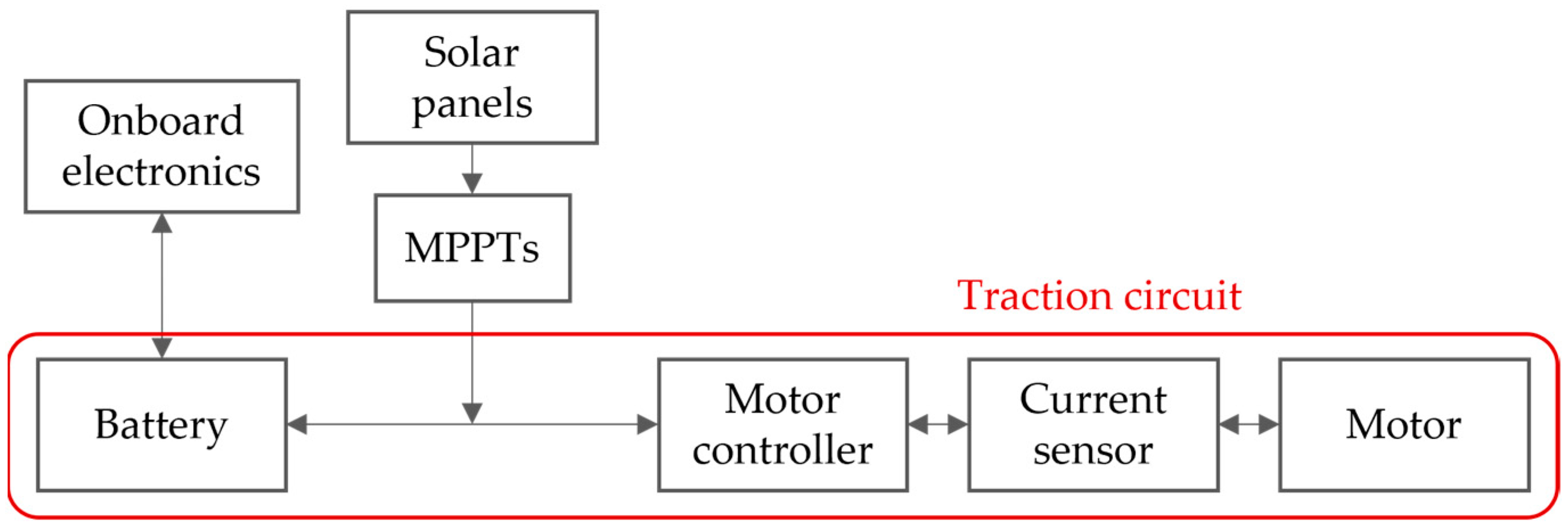
The first step was to create a model of the SEV that was as accurate as possible. The creation of this model was performed in MATLAB. The energy consumption model was created using Equations (1)–(3), (6), (7) and (9). This model can be seen in Equation (8) and is validated by its use in other relevant research [6,7,12,13].

Noticeably, every variable in these equations is either a constant, a measured value, or a calculated value, except for the C_d and C_r components.

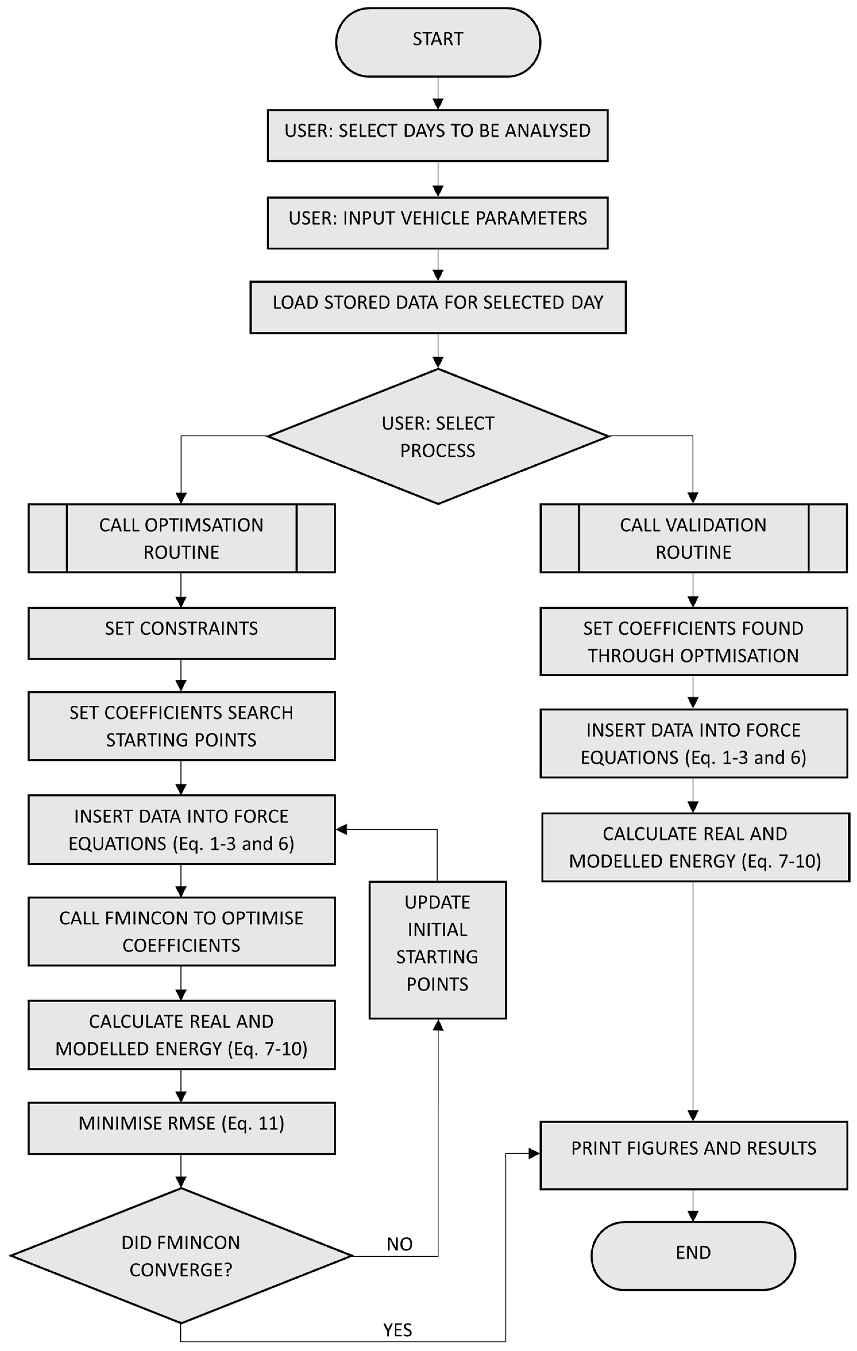
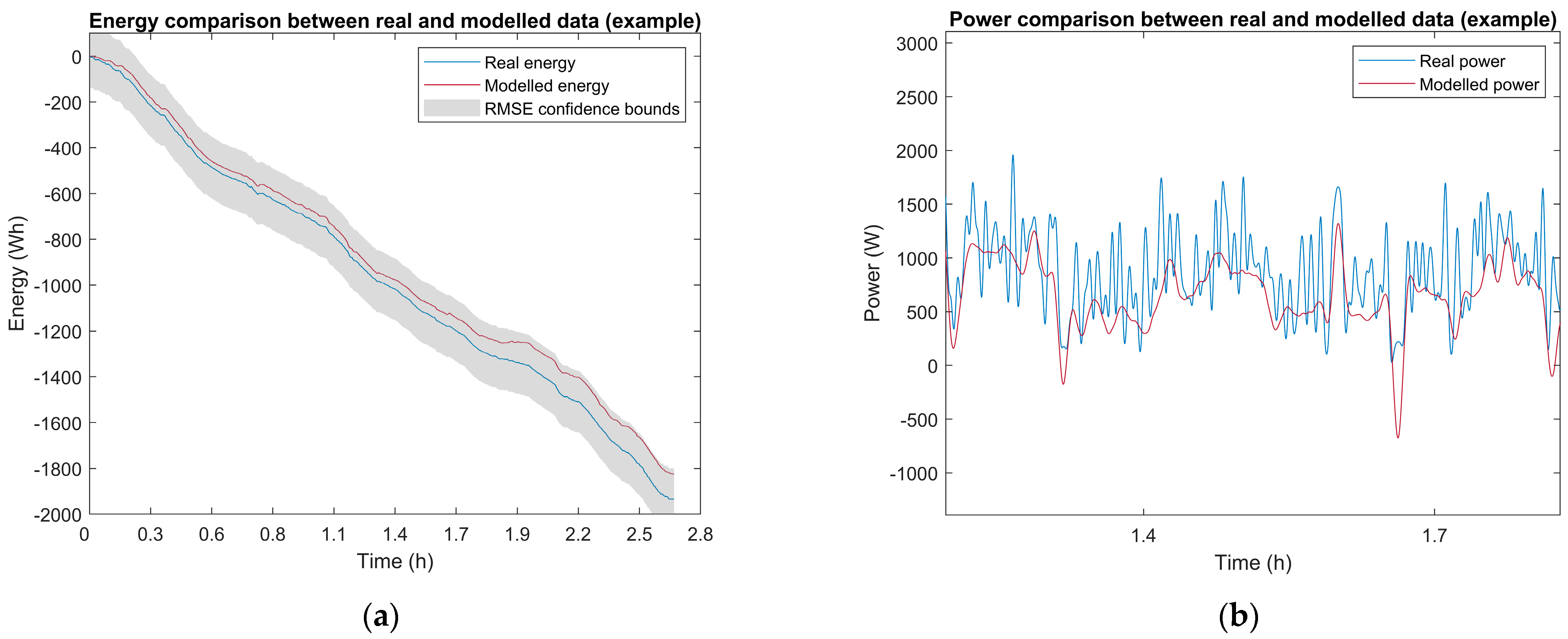
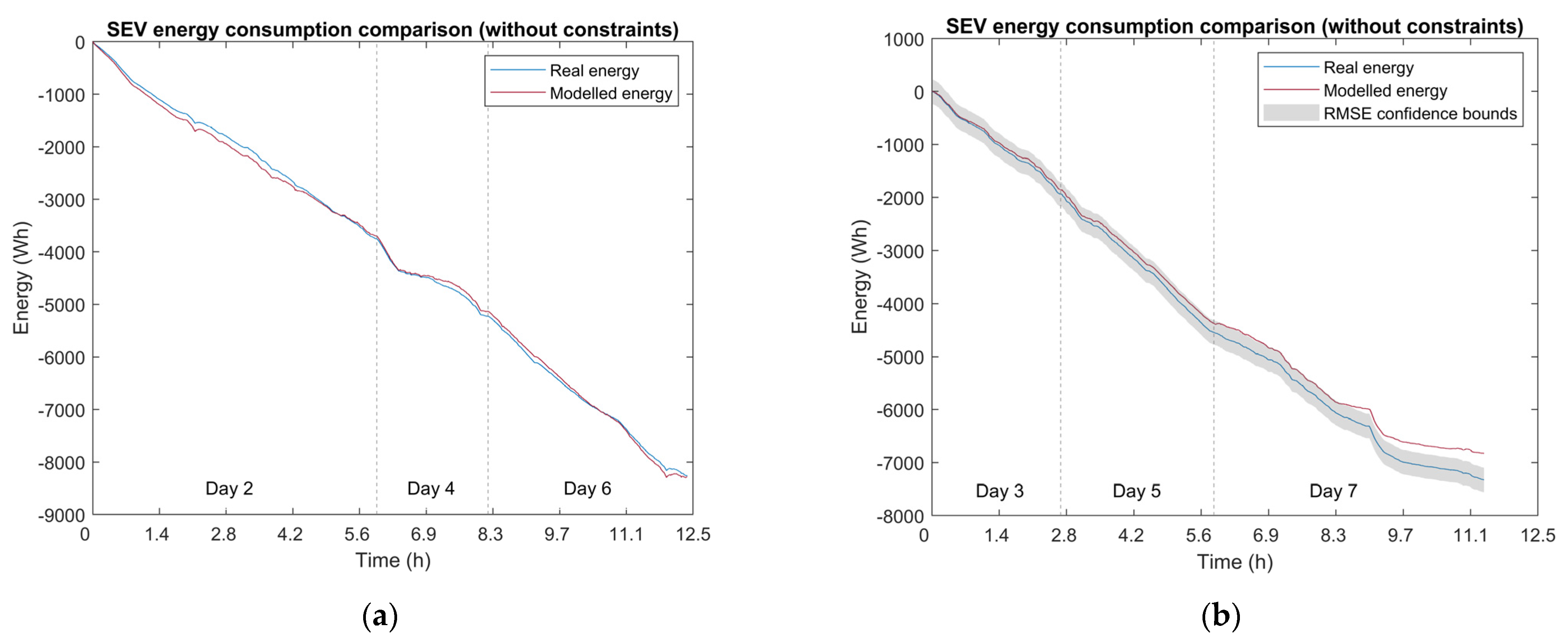
The optimisation process could then be attempted while using the modelled and real energies of the SEV. Figure 7a shows the results of the first test using the optimisation algorithm. Here, the energy calculated using the model (Equation (8)) and the real energy used by the SEV (Equation (10)) are plotted against each other. The RMSE between the two energies was minimised and determined which values of the coefficients best fit this optimal error.

In Figure 7a, the curves are very close together with an RMSE of 88 Wh. This indicates a very good relationship between the modelled and real energies. The C_d and C_r values found from the minimisation process are 0.0044 and 0.0131, respectively. However, this shows that the coefficients are far off from what was expected according to typical values, as seen in Table 6 and Table 7. The RMSE confidence bounds also show this. The final value of the modelled energy is outside the statistical mean forecasted error. There are a few factors at play here in the inaccuracy of the coefficients. Specifically, the non-dynamic model of the electric motor, different weights of the SEV drivers during the trip, variations in tyre pressure and bearing wear, crosswinds, road surface, and other unmodelled components contributed to this.

The first significant factor that influenced the undesirable results involved the modelling of the SEV’s electric motor. A complete dynamic model of the electric motor is required to determine its inefficiencies at different load and revolution-per-minute (RPM) rates. This is because the motor’s efficiency is determined by its torque and speed (RPM) at any given moment. Many factors (such as the inclination of the road) can change the torque and RPM of the motor. Since a dynamic efficiency map of the motor did not exist, the dynamic efficiency of the motor was not known at the time of this work. Therefore, a constant was chosen to represent the efficiency of the motor. The efficiency constant selected for the motor was 80%, as this was the value used for the same motor in a similar paper [22], and it is the average motor efficiency as supplied by the motor manufacturer.

Another factor that affected the coefficient values was the mass of the driver. To reduce driver fatigue, two drivers were used throughout the trip. The mass of the first driver was 80 kg, and that of the second driver was 63 kg. As the SEV already had a low mass, this mass variation would have significantly affected the vehicle’s behaviour. Unfortunately, it was not recorded when each driver was driving the vehicle. This, therefore, added to the discrepancies in the coefficients found via the optimisation routine. The mass of the heavier driver was used in this research as a worst-case scenario.

Variations in tyre pressure and bearing wear also influenced the coefficients. Tyre pressure can fluctuate as a result of heat or road surface, affecting the C_r value. Bearing wear also plays a role.

Crosswinds and wind gusts could also affect the C_d parameter. Although wind was considered in creating the model, it was difficult to determine the full effects of these wind gusts and crosswinds. For example, during heavy cross winds, the amount of tyre scrub increased dramatically as the vehicle underwent micro-sliding from left to right rather than just forward or backward (as a result of the car’s lightweight design). The micro-sliding caused significant wear to the tyres and affected their rolling resistance forces.

The road surface was also important. A road trip over 2000 km through two countries means that different road development and maintenance standards existed throughout.

Many less significant factors were unmodelled, as it would have been challenging to incorporate them and they would have made computation unnecessarily complex.

A similar energy model has been shown to be accurate and has been tested extensively in other research [13,22]. These concluded that omitting similar unmodelled components would not affect the results significantly. Thus, the coefficients found via the optimiser without constraints include all of these unmodelled components as well as the actual values for C_d and C_r. The optimiser without constraints tried to compensate for all discrepancies in the energy comparison by manipulating the C_d and C_r values accordingly.

These coefficients were then used on the validation data to determine their accuracy. The validation data are a concatenation of Days 3, 5, and 7. The results can be seen in Figure 7b. The validation of the unrealistic coefficients produced an RMSE of 232 Wh, translating to a final error value of 7.25%. This error value means that using three days of data to optimise the coefficients results in a final error value of 7.25%, according to these data. The final error value is the error value found at the end of Day 7 (the end of the trip). This is the final deviation that the user of the vehicle would experience in the state of charge between what was predicted and what is seen at the end of a trip.

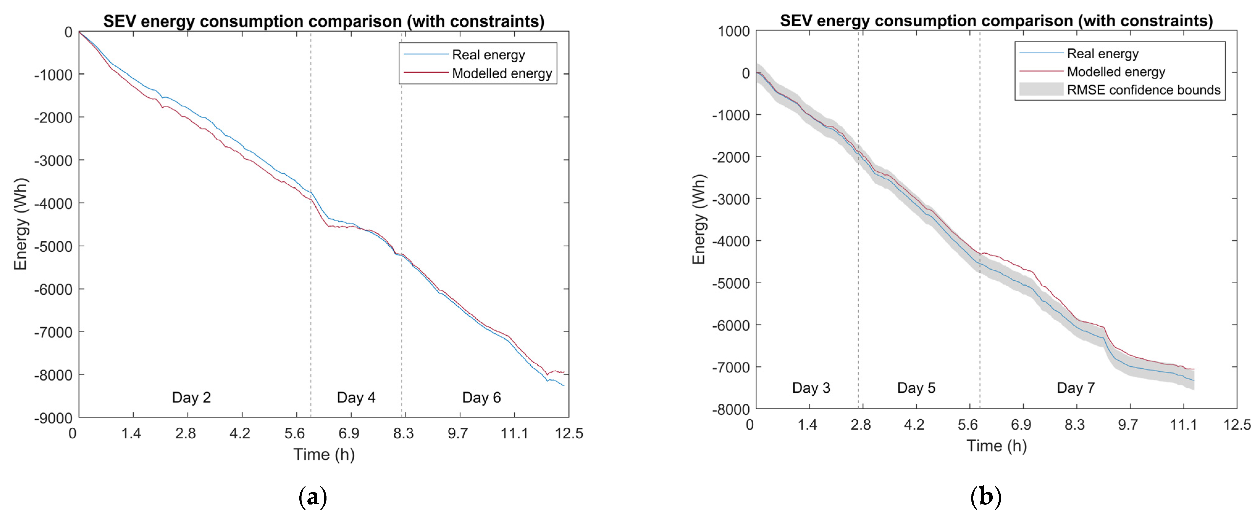
Because of the unrealistic coefficients, constraints were added to the optimisation process. The constraints would limit the values of the coefficients within a specific, realistic range. These constraints can be seen in Equation (11) and were chosen based on known realistic values for C_d and C_r, which can be seen in Table 6 and Table 7. The graph of the minimisation of the RMSE between the two energies can be seen in Figure 8a. This is from the same optimisation data set from Days 2, 4, and 6 used above.

Using constraints, the RMSE increased, but the values for the coefficients were far more realistic. The RMSE value was 161 Wh, and the C_d and C_r values were 0.13 and 0.0059, respectively. It can be noted that the value found for C_d does reach the lower bound of its constraint. This is due to the fact that the optimisation algorithm was still attempting to minimise the error towards the RMSE value found when no constraints were added. This is acceptable for this research as the lower bound of the constraint is a realistic value for C_d. As confirmation of this, the lower bound coefficient value is justified by the results of a CFD analysis found for the same vehicle performed by the members of the TUT solar car team [35]. A part of the modelled energy profile still exceeded the RMSE confidence interval, most likely because of the unmodelled components, as discussed above. However, it still provides a statistical error range for consideration by the user (in this case, the energy manager, or when this method is applied to other EVs, it might be the vehicle driver). The confidence interval was intentionally omitted from the optimisation results (Figure 8a), as visual error quantification is more applicable to the validation results.

With realistic values having been found for C_d and C_r using the optimisation data, it was then possible to test them on the validation data from Days 3, 5, and 7. The values of 0.13 for the C_d component and 0.0059 for the C_r component were inserted into the model of the SEV. With all model components known, the energy according to the model could be compared against the real (actual) energy. This was to validate the coefficients. The energy comparison can be seen in Figure 8b.

The validation of the realistic coefficients produced an RMSE of 217 Wh, which translates to a final error value of 4.12%. This contrasts with the 7.25% found using the unrealistic coefficients when no constraints were added. This further confirms that using the optimisation constraints provides realistic results (with a lower final error value); therefore, optimisation cannot be performed without adequate constraints.

3.2. Discussion of the Parameters That Affect the Model’s Performance

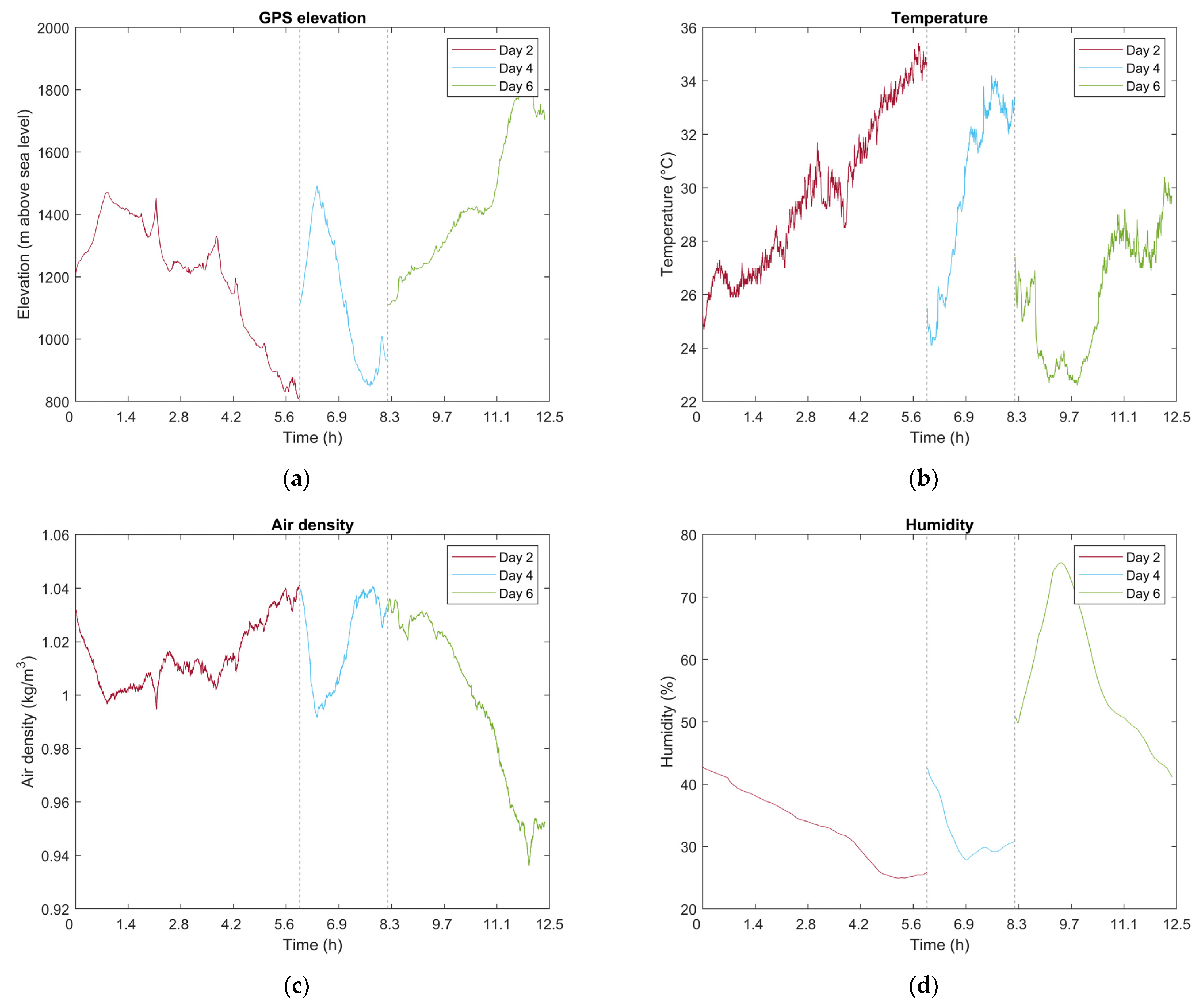
Multiple areas of interest in Figure 7 and Figure 8 show where and why the energies diverged. These could be attributed to certain environmental conditions. The conditions for Days 2, 4, and 6 can be seen in Figure 9.

Table 8. Amount of time spent travelling on each day (refer to Figure 9).

Day	Colour	Time Range (s)	Time Range (h)	Time Length (h:m:s)
2	Red	0–21,285	0–5.9	5:54:45
4	Blue	21,286–29,632	5.9–8.2	2:19:07
6	Green	29,633–44,571	8.2–12.4	4:08:59
Total	-	0–44,571	0–12.4	12:22:51

displays the time range and time spent driving each day. This table refers to the information found in Figure 9 and represents Days 2, 4, and 6.

Day 2 is characterised by an initial road climb followed by a long descent. It was a warm day with a stable air density (Figure 9c) and low humidity (Figure 9d). Air density is affected by temperature, pressure, and humidity and plays an important role in a vehicle’s drag force, as seen in Equation (1). The high altitude (Figure 9a) resulted in a lower drag force throughout the day. As the air density remained relatively constant, the drag force did not fluctuate as a result of the environmental conditions. Therefore, the gravity force affected the energy loss/gain the most. It can be seen in Figure 8a that the energies diverged almost immediately as a result of the gravity force. The real amount of energy used was higher than what the model predicted. This is most likely due to the lack of a motor model, as the efficiency of a motor varies based on the road’s incline (torque demand). Day 4 is characterised by a sharp uphill followed by a sharp downhill. As the vehicle gained elevation, the air density dropped. This lowered the drag force as a result of the thinning of the air. The temperature profile of Day 4 (Figure 9b) was very similar to Day 2. There was also very low humidity (Figure 9d). The drag and gravity forces would have affected the total energy loss/gain. The effects of this sharp climb on Day 4 can be seen in Figure 8a. The energy loss, according to the real and modelled data, showed the same trend. First, extra energy was consumed as the SEV ascended, followed by very little energy loss as the vehicle descended. Day 6 corresponds to a large and steady incline throughout the day. This took the SEV to the highest point of the trip. As in Day 4, when the elevation increased, the air density decreased. Therefore, the effects of the drag force decreased throughout the day, but there was a significant and stable gravitational force as a result of the increase in elevation. The lower temperature (Figure 9b) and high humidity (Figure 9d) also affected the air density (Figure 9c). The sudden decrease in elevation at the end of the day is also visible in Figure 8a. As the SEV decreased in altitude, its use of energy also decreased.

From looking at the elevation profiles (Figure 9a), it can be seen that the divergence between the actual and modelled energies is mainly attributed to changes in elevation. Although the divergence between energies is directly correlated to elevation, this is not the reason for the separation. The blue curve in Figure 7 and Figure 8 shows the SEV’s real energy usage. The divergence, therefore, most likely comes from the inaccuracies of the modelled energy. This confirms a relationship between the divergence observed and the factors mentioned above. The main reason for this is most likely that there was no dynamic motor efficiency model. The motor efficiency was set at a constant 80%; however, this was not always the case, especially when considering elevation changes. A significant incline (seen in all the elevation profiles in Figure 9) places a large amount of torque on a motor while speed (RPM) decreases or remains low. Most electric motors have a very low efficiency at high torque and low RPM. This is, therefore, not considered in the model as it results in visible deviations in the energies. The variations in driver mass also create inaccuracies as the gravity force will increase or decrease depending on this mass change.

There are also interesting areas in Figure 7b and Figure 8b. These represent the data from Days 3, 5, and 7.

Table 9. Time spent travelling each day (refer to Figure 10).

Day	Colour	Time Range (s)	Time Range (h)	Time Length (h:m:s)
3	Red	0–9568	0–2.7	2:39:28
5	Blue	9569–20,941	2.7–5.8	3:09:33
7	Green	20,942–41,000	5.8–11.4	5:34:19
Total	-	0–41,000	0–11.4	11:23:20

displays the time spent and the range of time driving on each day. This table refers to the information found in Figure 10 and represents Days 3, 5, and 7.

Day 3 was relatively short as it included the border crossing into Namibia from South Africa. It can be seen from the elevation profile in Figure 10a that the elevation jumped to a higher altitude instantaneously, in around 6000 s. This resulted from moving the SEV around 100 km on a trailer after the border post. As this day was relatively short, it did not have that much of an impact on the divergence between the energies. This means that the coefficients were a reasonably accurate prediction on Day 3. The altitude did not change much (Figure 10a), and the air density (Figure 10c) was quite constant. Therefore, the drag was relatively stable. This day was also characterised by the highest temperatures (Figure 10b) of the trip and low humidity (Figure 10d).

The elevation profile of Day 5 can be seen in Figure 10a. It followed the same trend as Day 3. The air density (Figure 10c) did not change much, with the elevation staying relatively constant and the humidity (Figure 10d) staying low. However, the temperature (Figure 10b) was slightly lower than it was on Day 3.

The elevation profile of Day 7 can be seen in Figure 10a. This shows an overall descent across the day from the inland parts of Namibia down to sea level. As the vehicle approached sea level, the air density (Figure 10c) and humidity (Figure 10d) increased. This was expected, as air becomes denser at lower altitudes and humidity rises closer to the sea. The temperature (Figure 10b) remained low throughout the day. This increase in air density played a role in the drag force, and the variable gravity force (no knowledge of which driver was in the vehicle at a time) from descending caused the energies to diverge, as seen in Figure 8b. The efficiency of the motor is once again most likely the culprit for this divergence. At an incline or decline, the lack of a dynamic motor model makes the overall model less accurate. The model predicts less energy used than what was actually used.

3.3. Final Results for Optimisation and Validation

Table 10. Error metrics and results.

	Cd	Cr	RMSE (Wh)	Final Value Error (Wh)	Final Value Error (%)
Optimisation 1	0.0044	0.0131	88	18	0.22
Validation 1	0.0044	0.0131	232	531	7.25
Optimisation 2	0.13	0.0059	161	322	3.90
Validation 2	0.13	0.0059	217	301	4.12

¹ Without constraints. ² With constraints.

displays the overall error results of the optimisation and validation processes. The optimisation and validation results for the test with no constraints are shown first. This is the experiment with unrealistic coefficients. The optimisation process produced a very low RMSE, final error value in Wh, and percentage. This indicates that the optimisation routine worked very well. However, the coefficients are unrealistic because they are unbounded. The optimisation creates a false sense of accuracy. When validating the coefficients on the second data set, the RMSE increased to the highest value in the experiment. This is also evident in the final error percentage. Although the optimisation process worked well, the results are poor and unreliable without the constraints. The optimiser without constraints tried to compensate for the discrepancies in the energy used, and once the constraints were added, the results improved to become more realistic and reliable values. The RMSE and final error percentage between the two data sets did not vary by much, which inspires confidence in the values of coefficients found with applicable constraints. The overall final error value percentage for the coefficients with constraints remains higher, meaning these constraints are critical for the optimisation process.

The accurate knowledge of these coefficients has proved essential in further energy applications of the vehicle. These coefficients are used in energy planning and optimisation, thus dictating the optimal speed to travel at. This yielded the maximum distance travelled in the following Sasol Solar Challenge that took place in South Africa in late 2022. Mainly as a result of this study, the team performed the best locally and covered a distance of 2682 km over a period of eight days.

4. Conclusions

With an alternative, easy, and accurate method for determining the coefficients of aerodynamic drag and rolling resistance, expensive and tedious experimentation can be eliminated. This research has proven that it is possible to use a more straightforward method to obtain, on average, a less than 5% prediction error, signifying its success and applicability in the EV industry. The final error value prediction shows how accurate the estimation was given the determined coefficients. Accurately determining these coefficients can be very useful in creating a precise energy model for an EV. This, in turn, can assist in better approximations of the range of an EV, therefore reducing range anxiety and possibly increasing the adoption of such technology in local and international markets.

Future work might include characterising the unmodelled components, as discussed in this work, to represent the energy model more accurately. This further research can be conducted if more data are collected during another large-scale field test. A more accurate dynamic motor efficiency map and the re-creation of the optimisation script using open-source (freeware) software will ensure that this method is less expensive and easier to apply than traditional methods.

This research can also be used to encourage newly formed solar car teams when starting the development of their own vehicles, as it offers an easier and less expensive method for finding these coefficients for their own energy modelling purposes.

References

1. European Parliament. EU Ban on the Sale of New Petrol and Diesel Cars from 2035 Explained. Available online: https://www.europarl.europa.eu/news/en/headlines/economy/20221019STO44572/eu-ban-on-sale-of-new-petrol-and-diesel-cars-from-2035-explained/ (accessed on 18 February 2023).
2. European Parliament. Reducing Carbon Emissions: EU Targets and Measures. Available online: https://www.europarl.europa.eu/news/en/headlines/society/20180305STO99003/reducing-carbon-emissions-eu-targets-and-measures/ (accessed on 18 February 2023).
3. European Parliament. Green Deal: Key to a Climate-Neutral and Sustainable EU. Available online: https://www.europarl.europa.eu/news/en/headlines/society/20200618STO81513/green-deal-key-to-a-climate-neutral-and-sustainable-eu/ (accessed on 18 February 2023).
4. Rauh, N.; Franke, T.; Krems, J. Understanding the Impact of Electric Vehicle Driving Experience on Range Anxiety. J. Hum. Factors Ergon. Soc. 2014, 57, 177–187. [Google Scholar] [CrossRef] [PubMed]
5. Sasol Solar Challenge. Welcome to the Sasol Solar Challenge. Available online: https://www.solarchallenge.org.za/ (accessed on 29 March 2023).
6. Husain, I.; Islam, M. Design, Modeling and Simulation of an Electric Vehicle System. J. Passeng. Cars 1999, 108, 2168–2176. [Google Scholar] [CrossRef]
7. Luigi, F.; Tarsitano, D. Modeling of Full Electric and Hybrid Electric Vehicles. In New Generation of Electric Vehicles; Stevic, Z., Ed.; IntechOpen: London, UK, 2012; pp. 208–236. [Google Scholar]
8. Lekshmi, S.; Lal Priya, P. Mathematical modeling of Electric vehicles—A survey. Control Eng. Pract. 2019, 92, 104138. [Google Scholar] [CrossRef]
9. Sharmila, B.; Srinivasan, K.; Devasena, D.; Suresh, M.; Panchal, H.; Ashokkumar, R.; Meenakumari, R.; Kumarsadasivuni, K.; Rajnikant Shah, R. Modelling and performance analysis of electric vehicle. Int. J. Ambient. Energy 2021, 43, 5034–5040. [Google Scholar] [CrossRef]
10. Smith, B.; Olaru, D.; Jabeen, F.; Greaves, S. Electric vehicles adoption: Environmental enthusiast bias in discrete choice models. Transp. Res. Part D Transp. Environ. 2017, 51, 290–303. [Google Scholar] [CrossRef]
11. Daina, N.; Sivakumar, A.; Polak, J. Modelling electric vehicles use: A survey on the methods. Renew. Sustain. Energy Rev. 2017, 68, 447–460. [Google Scholar] [CrossRef]
12. Hesami, S.; De Cauwer, C.; Rombaut, E.; Vanhaverbeke, L.; Coosemans, T. Energy-Optimal Speed Control for Autonomous Electric Vehicles Up- and Downstream of a Signalized Intersection. World Electr. Veh. J. 2023, 14, 55. [Google Scholar] [CrossRef]
13. Oosthuizen, C.; van Wyk, B.; Hamam, Y. Modelling and Simulation of the South African Designed Sun Chaser II Solar Vehicle. In Proceedings of the 2017 IEEE AFRICON, Cape Town, South Africa, 18–20 September 2017; pp. 1149–1154. [Google Scholar]
14. Martins, J.; Ning, A. Engineering Design Optimization; Cambridge University Press: Cambridge, UK, 2021. [Google Scholar]
15. Fahsl, C.; Vogt, P. Determination of the drag resistance coefficients of different vehicles. In The Physics Teacher; Springer: Cham, Switzerland, 2018; Volume 56. [Google Scholar]
16. Anderson, L.; Larsen, J. Introducing Functional Data Analysis to Coast Down Modeling for Rolling Resistance Estimation. SAE Int. J. Passeng. Cars 2015, 8, 786–796. [Google Scholar] [CrossRef]
17. Huertas, J.I. Accuracy and precision of the drag and rolling resistance coefficients obtained by on road coast down tests. In Proceedings of the International Conference on Industrial Engineering and Operations Management, Bogota, Colombia, 25–26 October 2017; pp. 575–582. [Google Scholar]
18. Anderson, L.; Larsen, J. Rolling Resistance Measurement and Model Development. J. Transp. Eng. 2014, 141, 04014075. [Google Scholar] [CrossRef]
19. MathWorks. Fmincon—Find Minimum of Constrained Nonlinear Multivariable Function. Available online: https://www.mathworks.com/help/optim/ug/fmincon.html (accessed on 24 April 2023).
20. Boggs, P.; Tolle, J. Sequential quadratic programming for large-scale nonlinear optimisation. J. Comput. Appl. Math. 2000, 124, 123–137. [Google Scholar] [CrossRef]
21. MathWorks. Choosing the Algorithm. Available online: https://www.mathworks.com/help/optim/ug/choosing-the-algorithm.html#brppuoz (accessed on 8 May 2023).
22. Oosthuizen, C.; van Wyk, B.; Hamam, Y.; Desai, D.; Alayli, Y.; Lot, R. Solar Electric Vehicle Energy Optimization for the Sasol Solar Challenge 2018. IEEE Access 2019, 7, 175143–175158. [Google Scholar] [CrossRef]
23. Mruzek, M.; Gajdáč, I.; Kučera, Ľ.; Barta, D. Analysis of Parameters Influencing Electric Vehicle Range. Procedia Eng. 2016, 134, 165–174. [Google Scholar] [CrossRef]
24. Szumska, E.; Jurecki, R. Parameters Influencing on Electric Vehicle Range. Energies 2021, 14, 4821. [Google Scholar] [CrossRef]
25. Kiyakli, A.O.; Solmaz, H. Modeling of an Electric Vehicle with MATLAB/Simulink. Int. J. Automot. Sci. Technol. 2018, 2, 9–15. [Google Scholar] [CrossRef]
26. Ejsmont, J.; Owczarzak, W. Engineering method of tire rolling resistance evaluation. Measurement 2019, 145, 144–149. [Google Scholar] [CrossRef]
27. Mavlonov, J.; Ruzimov, S.; Tonoli, A.; Amati, N.; Mukhitdinov, A. Sensitivity Analysis of Electric Energy Consumption in Battery Electric Vehicles with Different Electric Motors. World Electr. Veh. J. 2023, 14, 36. [Google Scholar] [CrossRef]
28. Asamer, J.; Graser, A.; Heilmann, B.; Ruthmair, M. Sensitivity analysis for energy demand estimation of electric vehicles. Transp. Res. Part D Transp. Environ. 2016, 46, 182–199. [Google Scholar] [CrossRef]
29. Tesla. Model S. Available online: https://www.tesla.com/models (accessed on 2 April 2023).
30. Browand, F.; McCallen, R.; Ross, J. The Aerodynamics of Heavy Vehicles II: Trucks, Buses, and Trains; Springer: Berlin/Heidelberg, Germany, 2009; Volume 41. [Google Scholar]
31. Banuri, S.H.A.S.; Qayyum, U.; Qureshi, K.R.; Ahmed, A. Investigation of Drag Coefficients for Various Car Models. In Proceedings of the 2020 17th International Bhurban Conference on Applied Sciences and Technology (IBCAST), Islamabad, Pakistan, 14–18 January 2020. [Google Scholar]
32. Tesla. Model X. Available online: https://www.tesla.com/modelx (accessed on 2 April 2023).
33. Aurora Vehicle Association Incorporated. Aurora Solar Car Team. Available online: http://www.aurorasolarcar.com/ (accessed on 10 May 2023).
34. Oosthuizen, C. Energy Optimisation of a Solar Vehicle for South African Conditions; Université Paris-Saclay; Tshwane University of Technology: Pretoria, South Africa, 2020. [Google Scholar]
35. TUT Solar Team. Sunchaser 4—A Technology Demonstration. Available online: https://sc4-technology.webflow.io/ (accessed on 20 April 2023).
36. Roche, D. Speed of Light: The 1996 World Solar Challenge; Photovoltaics Special Research Centre: Sydney, NSW, Australia, 1997; Volume 1. [Google Scholar]
37. X-Engineer. How to Calculate Rolling Resistance. Available online: https://x-engineer.org/rolling-resistance/ (accessed on 10 April 2023).
Figure 1. (a) TUTs fourth generation SEV; (b) SEV and support vehicle with weather station.
Wevj 14 00134 g001
Figure 2. Route map.
Wevj 14 00134 g002
Figure 3. Research methodology.
Wevj 14 00134 g003
Figure 4. SEV traction circuit.
Wevj 14 00134 g004
Figure 5. Examples: (a) energy comparison between real and modelled data; (b) power comparison between real and modelled data.
Wevj 14 00134 g005
Figure 6. MATLAB coding methodology.
Wevj 14 00134 g006
Figure 7. Using no constraints: (a) minimising the RMSE between real and modelled energy to determine Cd and Cr for the optimisation data set (days 2, 4, and 6); (b) validation of these coefficients on the second data set (days 3, 5, and 7).
Wevj 14 00134 g007
Figure 8. Using constraints: (a) minimising the RMSE between real and modelled energy to determine Cd and Cr for the optimisation data set (days 2, 4, and 6); (b) validation of these coefficients on the second data set (days 3, 5, and 7).
Wevj 14 00134 g008
Figure 9. Environmental conditions on Days 2, 4, and 6: (a) elevation; (b) temperature; (c) air density; (d) humidity.
Wevj 14 00134 g009
Figure 10. Environmental conditions on Days 3, 5, and 7: (a) elevation; (b) temperature; (c) air density; (d) humidity.
Wevj 14 00134 g010