Research on Trajectory Tracking Control of Driverless Electric Formula Racing Car Based on Game Theory

Abstract

A game theory based trajectory tracking control method is studied for the dual-objective optimization problem of trajectory tracking the accuracy and driving stability of driverless electric formula racing cars in high-speed trajectory conditions. The general control strategy and the model predictive controller based on the evolutionary game between the two players are designed to optimize their own decisions to achieve the optimal payoff for themselves, and to obtain the optimal solution to the dual-objective optimization problem, by taking the dual objectives of trajectory tracking accuracy and driving stability as the two players in the game. Considering the influence of the dynamic environment, the time-varying interactive game mechanism between two plays is introduced, the game payoff matrix is established, the weights of each subject are determined, and a dynamic replication system is constructed by weight evolution to find the optimal equilibrium strategy for the model prediction controller. The simulated results show that the designed controller can play a significant role in optimizing the trajectory tracking accuracy and driving stability compared to a single model predictive controller under different speed tracking conditions.

1. Introduction

Nowadays, driverless technology is developing at a high speed [1]. The high-speed trajectory of the driverless electric formula racing car is complex, with variable curvature, and is the most difficult event in the driverless electric formula racing car competition, with the highest scores and the most difficult problems to be solved to ensure trajectory tracking accuracy and driving stability. This paper is a study of driverless electric formula racing cars.

In the area of trajectory tracking control, domestic and foreign scholars have mainly conducted a lot of research on control theories such as linear optimal quadratic control (LQR) [2], model predictive control (MPC) [3,4], neural network control [5], preview BP neural network PID control [6], and feedback–feedforward control [7]. Ugo Rosolia et al. [8] proposed a two-loop approach to obstacle avoidance for controlling self-driving cars, tracking the road center line while avoiding obstacles to achieve accurate path tracking and stable driving of the car. Its outer loop uses a non-linear model predictive control method, and the inner loop uses a linear feedback controller based on an optimal preview distance. Sara Mata et al. [9] presented a robust model predictive control method for trajectory tracking of linear time-invariant monorail model vehicles, which improved lateral control accuracy and stability. A. M. Ribeiro et al. [10], based on the theory of sum-of-squares planning, proposed a non-linear state feedback control method to solve the lateral stability problem of four-wheeled vehicles. Ji Xuewu et al. [11] proposed an adaptive neural network-based robust lateral motion control of driving limits for autonomous vehicles, combining the adaptive control mechanisms of Lyapunov stability theory with radial basis function neural networks to improve the tracking yaw stability. Based on adaptive model predictive control theory and sliding mode variable structure control theory, Yunlong Bai et al. [12] designed a transverse-longitudinal cooperative controller to improve the trajectory tracking accuracy and driving stability of an unmanned racing car. Jie Su et al. [13] presented a time-varying controller optimization algorithm (TV-CON-OPT) for self-driving vehicles, which improved the control stability of the vehicle by taking into account the uncertainty between the system, the environment, and the uncertainty of the controller parameters. Ziniu Hu et al. [14] proposed an adaptive robust control (ARC), which guaranteed tracking stability and tracking accuracy for self-driving vehicles. Zhe Sun et al. [15] proposed a control strategy for fast non-singular terminal sliding modes of a dual hidden layer output feedback neural network for autonomous vehicles, which improved tracking accuracy, convergence speed, and stability. Peicheng Shi et al. [16] proposed an intelligent vehicle path-tracking control method based on improved model predictive control (MPC), combined with hybrid proportional-integral-derivative (PID) control theory, and improved the trajectory tracking accuracy and driving stability. Zhongchao Liang et al. [17] proposed an adaptive MPC trajectory tracking controller to improve robustness of the tracking process by continuously updating the Kalman state estimator correlation gain coefficient matrix, as well as the state of the controller, to ensure accuracy and stability. Ying Xu et al. [18] proposed a model predictive control (MPC) and preview-follower theory (PFT) to improve tracking accuracy and lateral stability. Bai Guoxing et al. [19] proposed a control law for improving the optimal prediction time domain and reference speed of a nonlinear model prediction controller to improve the control performance of vehicle path tracking. Kunwu Zhang et al. [20] proposed an adaptive learning model predictive control (ALMPC) scheme for trajectory tracking of perturbed autonomous ground vehicles (AGVs), subject to input constraints, which effectively reduced tracking errors and improved stability. Li Gang et al. [21] proposed a fuzzy controller based on optimal control theory and fuzzy logic method to design a two-motor differential drive fuzzy controller to improve the trajectory accuracy and timeliness of driverless electric racing cars. Di Ao et al. [22] proposed the development of super torsional sliding mode control algorithm (STA), based on Lyapunov theory, and demonstrated the stability of the control system by applying the back stepping technique to improve the autonomous vehicle to have smaller lateral error and smoother yaw rate. Guoqing Geng et al. [23] designed a trajectory tracking controller based on a neural network predictive control system (NNPC), which effectively improved the control accuracy and real-time performance of autonomous driving vehicles. Hongyu Jiao et al. [24] proposed an improved method of guiding weights without sensitivity analysis, which effectively carried out the optimal design.

In summary, the above research is based on linear optimal quadratic control, model predictive control, neural network control, and other control theories for trajectory tracking control that better solve the problems of trajectory tracking accuracy and driving stability. In order to solve the optimization problem of the dual-objective dynamic change with time and environment of the trajectory tracking accuracy and driving stability under high-speed tracking conditions and the weight problem, a model predictive controller based on the evolution game of both sides is designed. Both sides of the game player are in the process of optimizing the objective function, which allows tracking accuracy and driving stability to use the optimization of their own actions to maximize their own payoff and find the best solution to the optimization problem.

2. Game Theory Based on Trajectory Tracking Control Strategy

As shown in Figure 1, $Y_{ref}$ is the reference lateral displacement; ${\phi }_{ref}$ is the reference yaw angle; $\dot{y}$ and $\dot{x}$ are the speed of the vehicle in the y and x axis directions of the inertial coordinate system, respectively; $\phi$ is the yaw angle; $\dot{\phi }$ is the vehicle yaw rate; $Y$ is the lateral displacement; $X$ is the longitudinal displacement.

The driverless electric formula racing car decision planning layer plans the reference path, while the car collects its own state information through sensors to determine the difference between the position and the reference path, and solves the front wheel turning angle through the control algorithm and sends it to the line control steering system to make the driverless electric car follow the reference path. The model prediction is based on the input quantity of the system and the current state quantity, which is substituted into the prediction model to solve the state of the system in the future prediction time domain. Rolling optimization is performed by setting restrictive constraints on the system and an objective function, which is about trajectory tracking accuracy and driving stability. Consideration is given to the optimization problem of dynamic change with time and environment and the weighting problem between dual objectives, based on the theory of evolutionary game between two parties. Steps are then taken to determine the evolutionary game subject, establish the game gain matrix, determine the weight of each subject, and construct a dynamic replication system for weight evolution. The optimal equilibrium strategy is found for the solution of the model predictive controller, in which the optimization is carried out all the time. Then, a feedback correction is performed to execute the current moment’s control quantity for the trajectory tracking control of the driverless electric formula racing car.

3. Design of the Controller

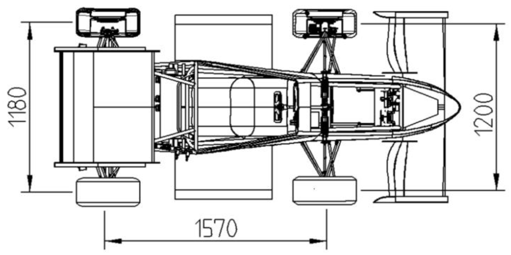
3.1. The Whole Vehicle Parameters of Driverless Electric Formula Racing Car

Table 1. Main parameters of the racing car.

Symbol	Parameters	Value	Units
m	Vehicle mass	260	kg
a	Distance from the center of mass to the front axis	706.5	mm
b	Distance from the center of mass to the rear axis	863.5	mm
L	Wheelbase of vehicle	1570	mm
${\mathrm{r}}_{\mathrm{r}}$	radius of wheel	228.6	mm
${\mathrm{h}}_{\mathrm{g}}$	Height of the center of mass	270	mm
${\mathrm{T}}_{\mathrm{f}}$	Gauge of the front axle	1200	mm
${\mathrm{T}}_{\mathrm{r}}$	Gauge of the rear axle	1180	mm

shows the main parameters of the whole vehicle. A sketch of the vehicle dimensions is shown in Figure 2.

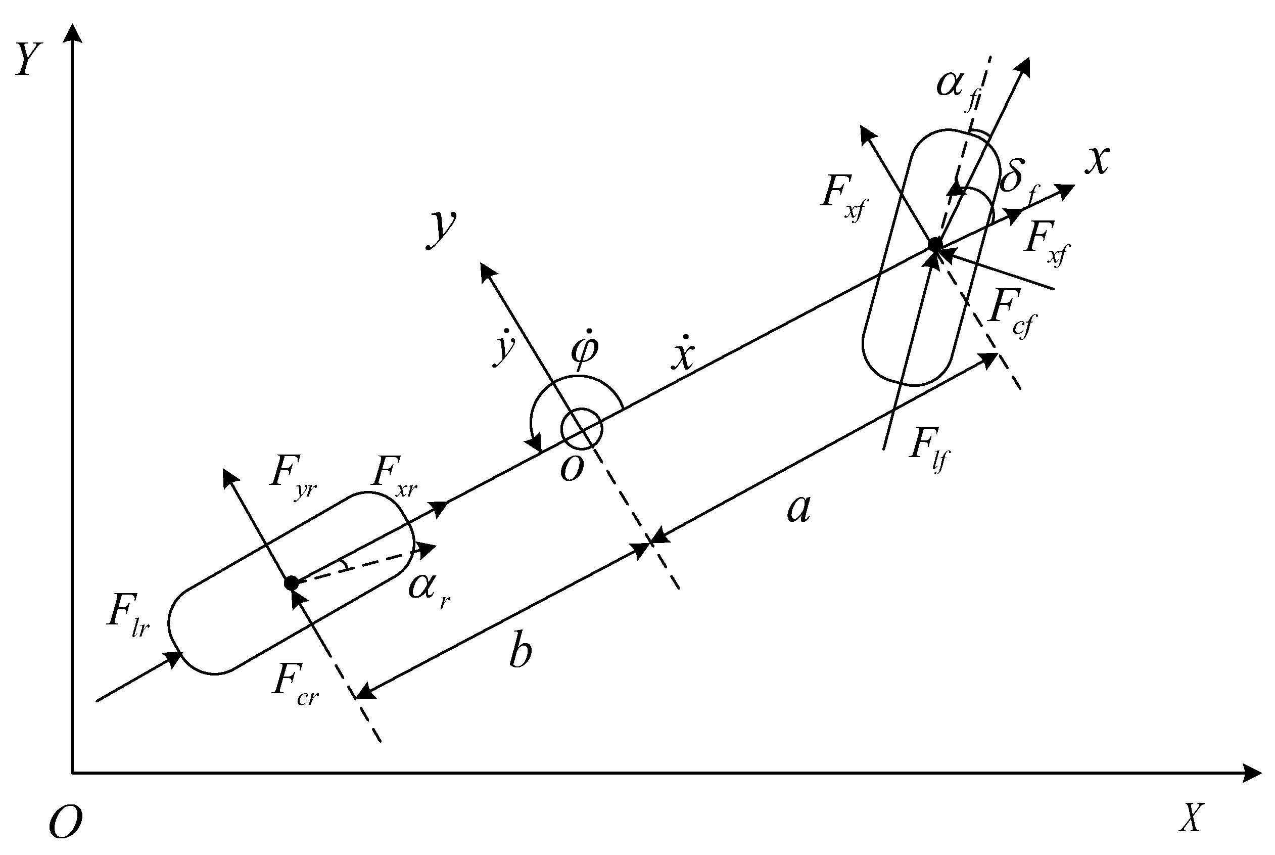
3.2. Vehicle Dynamics Modeling

The suspension system of the driverless electric formula racing car uses an electromechanical ISD suspension system, with reference to the optimal design method of vehicle electromechanical ISD suspension system based on fractional-order grid proposed by Yujie Shen et al. for improving the vibration resistance of the fractional-order ISD suspension [25]. Lithium battery pack reference to Jia Wang et al. Fault diagnosis method of lithium-ion battery pack using improved RBF neural network [26]. The design of permanent magnet motor is referred to the multi-objective optimization design of variable slope permanent magnet motor with driving cycle by Zhou X et al. [27].

Both the prediction model and the reference model of the model prediction controller use a vehicle three-degree-of-freedom dynamics model that considers only the longitudinal, lateral, and yaw motions of the driverless electric formula racing car. Assume that the road surface is smooth; only the front wheels are steered; ignore the drooping motion of the vehicle; ignore the suspension system and aerodynamics of the racing car; ignore the lateral load transfer of the tires; ignore the lateral-longitudinal coupling relationship of the tire forces and other conditions.

As shown in Figure 3, XOY is the inertial reference frame; xoy is the vehicle reference frame; the point O is the center of mass of the vehicle; x is the longitudinal direction of the body; y is the lateral direction of the body; ${\alpha }_f$ and ${\alpha }_r$ are the tire slip angle of the front and rear tire, respectively; ${\delta }_f$ is the steering angle of front wheels; a is the distance from the center of mass to the front axis; b is the distance from the center of mass to the rear axis; $\dot{y}$ and $\dot{x}$ is the speed of the vehicle in the y and x axis directions of the inertial coordinate system, respectively; $\dot{\phi }$ is the vehicle yaw rate; $F_{lf}$ and $F_{lr}$ is the longitudinal force of the front tire and rear tire, respectively; $F_{cf}$ and $F_{cr}$ is the lateral force of the front tire and rear tire, respectively.

According to Newton’s second law for the x-axis and y-axis and the balance of moments around the z-axis, we get Equation (1):

$$\{\begin{array}{l}m\ddot{x}=2F_{xf}+2F_{xr}+m\dot{y}\dot{\phi }\hfill \\ m\ddot{y}=2F_{yf}+2F_{yr}-m\dot{x}\dot{\phi }\hfill \\ I_z\ddot{\phi }=2a{F}_{yf}-2b{F}_{yr}\hfill \end{array}$$

(1)

where $\ddot{x}$ and $\ddot{y}$ are the acceleration of the vehicle in the x and y axis direction, respectively; $I_z$ is the moment of inertia of the vehicle, $I_z=340\mathrm{kg}·{\mathrm{m}}^2$; $\ddot{\phi }$ is the yaw angle acceleration.

3.3. Tire Force Analysis

The simplified “magical tire” formula is chosen to represent the longitudinal force and lateral force of the tire. For the two lateral forces on the tire, taking into account the small angle assumption [28], the lateral deflection force applied to the tire by the ground is linearly related to the lateral deflection angle of the tire, and the tire is subjected to Equation (2):

$$\{\begin{array}{l}{F}_{lf}=C_{lf}{S}_f\hfill \\ F_{lr}=C_{lr}{S}_r\hfill \\ F_{cf}=C_{cf}{\alpha }_f=C_{cf}({\delta }_f-\frac{\dot{y}+a\dot{\phi }}{\dot{x}})\hfill \\ F_{cr}=C_{cr}{\alpha }_r=C_{cr}(\frac{b\dot{\phi }-\dot{y}}{\dot{x}})\hfill \end{array}$$

(2)

where $C_{lf}$ and $C_{lr}$ are the longitudinal stiffness of front and rear tires, respectively, $C_{lf}=C_{lr}=35,000$ N/rad; $S_f$ and $S_r$ are the slip rate of the front and rear tires, respectively, $S_f=S_r=0.2$; $C_{cf}$ and $C_{cr}$ are the lateral stiffness of front and rear tires, respectively, $C_{cf}=C_{cr}=51,000$ N/rad. Finally, by substituting Equation (2) into Equation (1) and transforming between the vehicle reference frame and the inertial reference frame, the dynamic equation of the vehicle is obtained as Equation (3):

$$\{\begin{array}{l}\ddot{x}=\frac{2}{m}[C_{lf}{S}_f-C_{cf}({\delta }_f-\frac{\dot{y}+a\dot{\phi }}{\dot{x}}){\delta }_f+C_{lr}{S}_r]+\dot{y}\dot{\phi }\\ \ddot{y}=\frac{2}{m}[C_{cf}({\delta }_f-\frac{\dot{y}+a\dot{\phi }}{\dot{x}})+C_{cr}(\frac{b\dot{\phi }-\dot{y}}{\dot{x}})]-\dot{x}\dot{\phi }\hfill \\ \ddot{\phi }=\frac{2}{I_z}[a(C_{cf}({\delta }_f-\frac{\dot{y}+a\dot{\phi }}{\dot{x}})-b{C}_{cr}(\frac{b\dot{\phi }-\dot{y}}{\dot{x}})]\hfill \\ \dot{Y}=\dot{x}\sin \phi +\dot{y}\cos \phi \hfill \\ \dot{X}=\dot{x}\cos \phi -\dot{y}\sin \phi \hfill \\ \dot{\phi }=r\end{array}$$

(3)

where $\dot{X}$ and $\dot{Y}$ are the velocities of the vehicle in the X-axis and Y-axis directions of the inertial reference frame; r denotes the angular velocity around the Z-axis.

3.4. Design of Model Predictive Controller

Model predictive control is the use of existing predictive models, the current state of the system, and future control quantities to predict the future output of the system through rolling optimization to solve the problem with constraints to achieve control purposes [29].

Transformation of the vehicle three-degree-of-freedom dynamics model into state space is expressed as Equation (4):

$$\{\begin{array}{l}\dot{\mathit{\xi }}=f(\mathit{\xi },\mathit{u})\hfill \\ \mathit{\lambda }=C·\mathit{\xi }\hfill \end{array}$$

(4)

where $\mathit{\xi }$ is the state quantity, $\mathit{\xi }={\left[\dot{y},\dot{x},\phi ,r,Y,X\right]}^T$; u is a control quantity, $\mathit{u}=\left[{\delta }_f\right]$; $\mathit{\lambda }$ is the output, $\mathit{\lambda }={\left[\phi ,Y\right]}^T$.

Linearization of the vehicle model introduces the first-order Taylor formula and leads to Equation (5):

$$\dot{\xi }=f({\xi }_{r,}{u}_r)+A(t)(\xi -{\xi }_r)+B(t)(u-u_r)$$

(5)

where $f({\xi }_{r,}{u}_r)$ denotes the value of the function $\dot{\xi }$ at the reference point $({\xi }_{r,}{u}_r)$.

Find the Jacobi matrix as Equation (6):

$$A(t)=\frac{\partial f(\xi (t),u(t))}{\partial \xi },B(t)=\frac{\partial f(\xi (t),u(t))}{\partial u}$$

(6)

The system is discretized using the forward Euler method as Equation (7):

$$\dot{\xi }(k)=\frac{\xi (k+1)-\xi (k)}{T}=A(t)\xi (k)+B(t)u(k)$$

(7)

The state space equation is obtained as Equation (8):

$$\xi (k+1)=A_k\xi (k)+B_{k}u(k)$$

(8)

where T denotes the time increment between the moment k + 1 and the moment k. Where $A(k)=I+TA(t)$, $B(k)=TB(t)$.

To ensure smoothness in the control process, select the amount of change in front wheel angle control to limit the control increment, and convert to Equation (9):

$$\{\begin{array}{l}\tilde{\xi }(k+1\mid t)={\tilde{A}}_{k,t}\tilde{\xi }(k\mid t)+{\tilde{B}}_{k,t}\Delta u(k\mid t)\hfill \\ \tilde{\lambda }(k\mid t)={\tilde{C}}_{k,t}\tilde{\xi }(k\mid t)\hfill \end{array}$$

(9)

where ${\tilde{A}}_{k,t}=\left[\begin{array}{cc}{A}_{k,t}& B_{k,t}\\ 0& I\end{array}\right]$, ${\tilde{B}}_{k,t}=\left[\begin{array}{c}{B}_{k,t}\\ I\end{array}\right]$, $\lambda (k\mid t)$ is the output of the system at time k, ${\tilde{C}}_{k,t}=\left[\begin{array}{cc}{C}_{k,t}& 0\end{array}\right]$, $C_{k,t}=\left[\begin{array}{l}\begin{array}{cccccc}0& 0& 1& 0& 0& 0\end{array}\\ \begin{array}{cccccc}0& 0& 0& 0& 1& 0\end{array}\end{array}\right]$, $\tilde{\xi }(k\mid t)=\left[\begin{array}{c}\xi (k\mid t)\\ u(k-1\mid t)\end{array}\right]$, $\Delta u(k\mid t)$ is the control increment at time k of the system, $\Delta u(k\mid t)=u(k\mid t)-u(k-1\mid t)$.

Let the prediction step of the MPC controller be Np and the control step be Nc, then the predicted output is Equation (10):

$$Y(k)={\psi }_k\tilde{\xi }(k|t)+{\Theta }_k\Delta u(k|t)$$

(10)

where $Y(k)=\left[\begin{array}{c}\tilde{\lambda }(k+1|t)\\ \tilde{\lambda }(k+2|t)\\ ⋮\\ \tilde{\lambda }(k+N_p|t)\end{array}\right]$, $\Delta U(k)=\left[\begin{array}{c}\Delta u(k|t)\\ \Delta u(k+1|t)\\ ⋮\\ \Delta u(k+N_c-1|t)\end{array}\right]$, ${\psi }_k=\left[\begin{array}{c}{\tilde{C}}_{k,t}{\tilde{A}}_{k,t}\\ {\tilde{C}}_{k,t}{\tilde{A}}_{k,t}^2\\ ⋮\\ {\tilde{C}}_{k,t}{\tilde{A}}_{k,t}^{N_p}\end{array}\right]$,

$${\Theta }_k=\left[\begin{array}{cccc}{\tilde{C}}_{k,t}{\tilde{B}}_{k,t}& 0& \cdots & 0\\ {\tilde{C}}_{k,t}{\tilde{A}}_{k,t}{\tilde{B}}_{k,t}& {\tilde{C}}_{k,t}{\tilde{B}}_{k,t}& \cdots & 0\\ ⋮& ⋮& ⋮& ⋮\\ {\tilde{C}}_{k,t}{\tilde{A}}_{k,t}{}^{N_c-1}{\tilde{B}}_{k,t}& {\tilde{C}}_{k,t}{\tilde{A}}_{k,t}{}^{N_c-2}{\tilde{B}}_{k,t}& \cdots & {\tilde{C}}_{k,t}{\tilde{B}}_{k,t}\\ {\tilde{C}}_{k,t}{\tilde{A}}_{k,t}{}^{N_c}{\tilde{B}}_{k,t}& {\tilde{C}}_{k,t}{\tilde{A}}_{k,t}{}^{N_c-1}{\tilde{B}}_{k,t}& \cdots & {\tilde{C}}_{k,t}{\tilde{A}}_{k,t}{\tilde{B}}_{k,t}\\ ⋮& ⋮& \ddots & ⋮\\ {\tilde{C}}_{k,t}{\tilde{A}}_{k,t}{}^{N_p-1}{\tilde{B}}_{k,t}& {\tilde{C}}_{k,t}{\tilde{A}}_{k,t}{}^{N_p-2}{\tilde{B}}_{k,t}& \cdots & {\tilde{C}}_{k,t}{\tilde{A}}_{k,t}{}^{N_p-N_c}{\tilde{B}}_{k,t}\end{array}\right]$$

(11)

Therefore, the amount of state at the current moment is known, and the control increment in the control time domain Nc, the amount of system output in the future prediction time domain Np can be predicted.

3.5. The Design Requirements of the Objective Function

1.

The tracking process maintains a small tracking error, and the error can converge to zero quickly and steadily, and remain balanced.

2.

The front wheel angle control input in the tracking process is as small as possible, and the change should be smooth.

Therefore, the objective function is designed as Equation (12):

$$J(\mathit{\xi }(k),\mathit{u}(k-1),\Delta \mathit{U}(k))={\displaystyle \sum _{i=1}^{N_p}||\tilde{\mathit{\lambda }}(k+i|t)-{\mathit{\lambda }}_{ref}(k+i|t)||\begin{array}{c}2\\ \mathit{Q}\end{array}}+{\displaystyle \sum _{i=1}^{N_c-1}||\Delta \mathit{u}(k+i|t)||\begin{array}{c}2\\ \mathit{R}\end{array}}+\rho {\epsilon }^2$$

(12)

where $\tilde{\mathit{\lambda }}(k+i|t)$ is the actual system state; ${\mathit{\lambda }}_{ref}(k+i|t)$ is the referenced system state; Q is the state weight coefficient matrix; R is the control increment weight coefficient matrix; Q and R play a large role in the optimization of the objective function, as will be explained in detail later in this section; $\rho$ is the relaxation factor weight coefficient; $\epsilon$ is the relaxation factor. Thus, the objective function transforms the problem into a quadratic programming solution problem as Equation (13):

$$J(\mathit{\xi }(k),\mathit{u}(k-1),\Delta \mathit{U}(k))=\frac{1}{2}{[\Delta \mathit{U}{(k)}^T,\epsilon ]}^T\mathit{H}[\Delta \mathit{U}{(k)}^T,\epsilon ]+\mathit{G}\left[\Delta \mathit{U}{(k)}^T,\epsilon \right]$$

(13)

where H and G are the coefficient matrices:

$$H=\left[\begin{array}{cc}2({\Theta }_k^{T}Q{\Theta }_K+R)& 0\\ 0& 2\rho \end{array}\right]G=\left[2E^T(k)Q{\Theta }_{k}0\right]$$

Constraints: considering the control amount and control increment of trajectory tracking, and the constraints of front wheel turning angle, the following constraints are to be satisfied in each control time domain are in Equation (14):

$$\{\begin{array}{l}{U}_{\min }⩽U_t⩽U_{\max }\\ \Delta U_{\min }⩽\Delta U_t⩽\Delta U_{\max }\\ y_{\mathrm{hc},}{}_{\min }\le y_{\mathrm{hc}}\le y_{\mathrm{hc},\max }\\ y_{\mathrm{sc},\min }-\epsilon \le y_{\mathrm{sc}}\le y_{\mathrm{sc},\max }+\epsilon \\ \min {\displaystyle \sum _{i=1}^{N_{\mathrm{p}}}{\Vert \mathsf{\eta }(t+i\mid t)-{\mathsf{\eta }}_{\mathrm{Tef}}(t+i\mid t)\Vert }_Q^2}+{\displaystyle \sum _{i=1}^{N_{\mathrm{c}}-1}\Vert \Delta u(}t+i\mid t){\Vert }_R^2+\rho {\epsilon }^2\end{array}$$

(14)

where $U_{\min }$ and $U_{\max }$ are the minimum and maximum values of the control input; $\Delta U_{\max }$ and $\Delta U_{\min }$ are the maximum and minimum values of the control input increment; $y_{\mathrm{hc},}{}_{\min }$ and $y_{\mathrm{hc},\max }$ are the minimum and maximum values of the hard constraint of output; $y_{\mathrm{sc},\min }$ and $y_{\mathrm{sc},\max }$ are the minimum and maximum values of the soft constraint of output. Calculating Equation (13) in each sampling period, the incremental front wheel rotation angle is obtained as Equation (15):

$$\Delta U_t^{*}={\left(\Delta u_t^{*},\Delta u_{t+1}^{*},\cdots ,\Delta u_{t+N_{\mathrm{c}}-1}^{*},\epsilon \right)}^{\mathrm{T}}$$

(15)

where $\Delta u_t^{*}$, $\Delta u_{t+1}^{*}$, $\cdots$, $\Delta u_{t+N_{\mathrm{c}}-1}^{*}$ are the system control inputs for moments $t$, $t+1$, $t+N_c-1$.

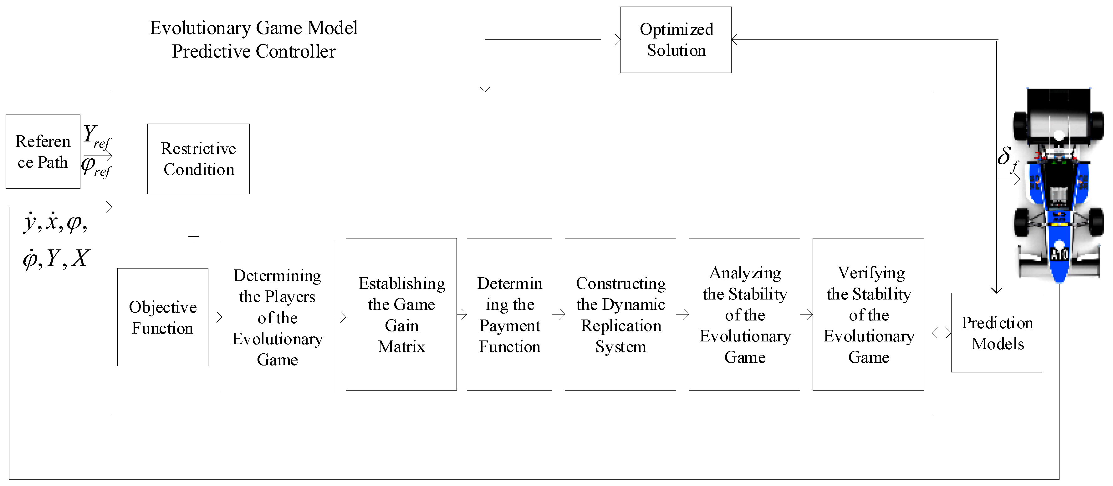
3.6. Evolutionary Game Model Predictive Controller Design

Traditional game: under certain conditions and in compliance with certain rules, one or several people or teams with absolute rational thinking choose and implement the behavior or strategy from which each is allowed to choose, and from which each achieves the corresponding result or gain.

Evolutionary games: instead of modeling the game as a super-rational game, it is believed that humans usually reach the game equilibrium by trial and error (dynamic), and evolutionary game theory does not require the participants to be perfectly rational (finite rationality), nor does it require the condition of complete information. The advantage of evolutionary games is that they can change trends over time and environment.

Equation (12) is a typical multi-objective optimal control problem, the objective function can be simplified to represent the weighting of the cumulative tracking deviation of the tracking process and the cumulative control input, as in Equation (16):

$$J={\displaystyle \sum _{k=1}^N\left(X^{T}QX+u^{T}Ru\right)}$$

(16)

where Q is a semi-positive definite weighting matrix and R is a positive definite control weighting matrix, both of which are diagonal arrays; larger elements of the Q matrix represent the desire for the tracking bias to quickly converge to zero, and the larger elements of the R matrix represent the control input to be as small as possible. In order to study the dynamic process in the trajectory tracking, the interaction between the two plays changes, and based on the adaptability of the strategy change, the “evolutionary stable strategy” (ESS) is adopted. As proposed in [30], in the repeated game, the participants will constantly adjust their interests to the optimal strategy by having incomplete information to reach an equilibrium, and changing the strategy again will not make any party get a better result.

3.6.1. Determining the Players of the Evolutionary Game

The optimization of the objective function of the optimization problem with two game players, in the framework of the evolutionary game, is achieved by designing a suitable payoff function for each player and using the players’ own optimization strategies to achieve the optimal solution of the objective function [31]. It is assumed that the strategy selection and dynamic adjustment of both sides of the evolutionary game follow the rule of finite rationality. The participants of the evolutionary game in this paper are the cumulative path deviation value Q of the tracing process and the loss of control energy R in the tracing process, and the strategy space is $S_1$ = (high precision, low precision), $S_2$ = (low stability, high stability)—see

Table 2. Players of the game.

Player	Q	R
Strategy space	$S_1$ = (High accuracy, Low accuracy)	$S_2$ = (Low stability, High stability)

.

3.6.2. Establishing the Game Gain Matrix

Choose a scale of y for high precision and 1 − y for low precision. The gain for R1 at high precision is A and the gain for R2 at low precision is B, see

Table 3. Gain matrix of the hybrid strategy game with Q and R.

		Tracing Process and the Loss of Control Energy R
		R1 Low stability (1 − x)	R2 High stability (x)
Cumulative path deviation value Q	Q1 Low accuracy (y)	(A,E)	(B,F)
	Q2 High accuracy (1 − y)	(C,G)	(D,H)

.

As shown in Table 3, R1 indicates that participant R takes a low-stability strategy, R2 indicates that participant R takes a high-stability strategy, Q1 indicates that participant Q takes a low-precision strategy, and Q2 indicates that participant Q takes a high-precision strategy. x indicates the probability when participant R takes an R2 strategy, 1 − x is the probability when participant R takes a strategy R1, y indicates the probability when participant Q takes a Q2 strategy, and 1 − y is the probability when participant Q adopts strategy Q1. Therefore, x and y are the strategy-stabilized equilibrium points of the evolutionary game Q and R, and both are between 0 and 1. The values of x and y vary with time.

A denotes the gain of Q1 with a high-precision, low-stability strategy. E denotes the gain of R1 with a high-precision, low-stability strategy. B denotes the gain of Q1 with high accuracy and high stability strategy. F denotes the gain of R2 with high precision and high stability strategy. C denotes the gain of Q2 with a low precision, low stability strategy. G denotes the gain of R1 with a low precision, low stability strategy. D denotes the gain of Q2 with a low precision, high stability strategy. H denotes the gain of R2 when the low-precision, high-stability strategy is adopted.

3.6.3. Determining the Payment Function

When player Q adopts the pure strategy, Q1 and Q2’s payment functions are as Equation (17):

$$E{Q}_1=A(1-x)+Bx,E{Q}_2=C(1-x)+Dx$$

(17)

The average payout for selecting strategies Q1 and Q2 with probabilities of y and 1 − y is Equation (18):

$$EQ=y[A(1-x)+Bx]+(1-y)[C(1-x)+Dx]$$

(18)

when participant R adopts pure strategies R1 and R2. Payment function is Equation (19):

$$E(R_1)=Ey+G(1-y),E(R_2)=Fy+H(1-y)$$

(19)

The average payout for selecting strategies B1 and B2 with probabilities of 1 − x and x is Equation (20):

$$E(R)=x[Fy+H(1-y)]+(1-x)[Ey+G(1-y)]$$

(20)

3.6.4. Constructing the Dynamic Replication System

Statistical results show that when the average payment of a particular strategy is higher than the average payment of a mixed strategy, he will tend to use this strategy more often [32].

Then, the adjustment equations of Q and R for y and x are as Equation (21):

$$\frac{dx}{dt}=x[E(R_2)-E(R)],\frac{dy}{dt}=x[E(Q_1)-E(Q)]$$

(21)

That is, the dynamic replication system for the cumulative path deviation value Q strategy selection is Equation (22):

$$F(x)=\frac{dx}{dt}=x(1-x)[(F-E+G-H)y-(G-H)]$$

(22)

The dynamic replication system chosen for the controlled energy loss R strategy is Equation (23):

$$G(x)=\frac{dy}{dt}=y(1-y)[(A-C)-x(A-B-C+D)]$$

(23)

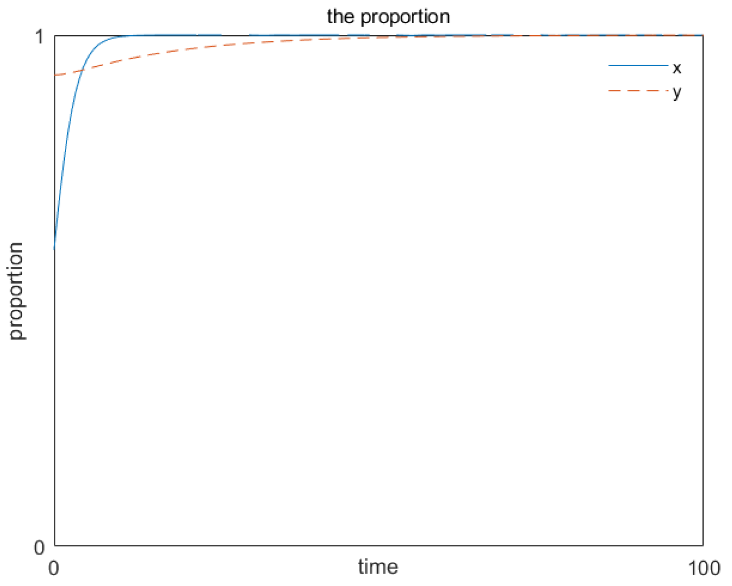
3.6.5. Analyzing the Stability of the Evolutionary Game

For any point $(x,y)\in [0,1]\times [0,1]$, therefore any point $(x,y)$ of the dynamic replication system corresponds to a mixed strategy even $((1-x)\oplus x,y\oplus (1-y))$ of the evolutionary game, and the combination of strategies corresponding to the equilibrium point is said to be an equilibrium of the evolutionary game, called the evolutionary equilibrium [33].

The evolutionary stability of the cumulative path deviation value Q and the control energy loss R are analyzed such that when $F(x)=G(x)=0$, the following five local equilibrium points are obtained: $G_1(0,1)$, $G_2(1,1)$, $G_3(0,0)$, $G_4(1,0)$, $G_5(x*,y*)$. Where $x*=\frac{A-C}{A-B-C+D}$, $y*=\frac{G-H}{F-E+G-H}$, ($0<(x*,y*)<1$). Using the Friedman method, $\det (J*)>0$, $tr(J*)<0$ stability analysis is done for dynamic replicated equilibrium points using Jacobi second-order matrix local stability.

The Jacobi matrix is Equation (24):

$$J*=\left[\begin{array}{l}\frac{\partial F(x)}{\partial x}\frac{\partial F(x)}{\partial y}\\ \frac{\partial G(y)}{\partial x}\frac{\partial G(y)}{\partial y}\end{array}\right]$$

(24)

where $\frac{\partial F(x)}{\partial x}=(1-2x)[(F-E+G-H)y-(G-H)]$, $\frac{\partial F(x)}{\partial \mathrm{y}}=x(1-x)(F-E+G-H)$, $\frac{\partial G(y)}{\partial x}=y(y-1)(A-B-C+D)$, $\frac{\partial G(y)}{\partial y}=(1-2y)[(A-C)-x(A-B-C+D)]$.

The determinant of the matrix $J*$ is Equation (25):

$$\begin{array}{l}\det (J*)=(1-2x)[(F-E+G-H)y-(G-H)](1-2y)[(A-C)-x(A-B-C+D)]\\ +x(1-x)(F-E+G-H)y(1-y)(A-B-C+D)\end{array}$$

(25)

The trace of the matrix is Equation (26):

$$tr(J*)=(1-2x)[(F-E+G-H)y-(G-H)]+(1-2y)[(A-C)-x(A-B-C+D)]$$

(26)

The stability points are brought into the matrix determinant and trace expressions to obtain

Table 4. Equilibrium point analysis.

Equilibrium Point	$\mathit{d}\mathit{e}\mathit{t}(\mathit{J}*)$	$\mathit{t}\mathit{r}(\mathit{J}*)$
$G_1(0,1)$	$(F-E)(C-A)$	$F-E+C-A$
$G_2(1,1)$	$(E-F)(D-B)$	$E-F+D-B$
$G_3(0,0)$	$(H-G)(A-C)$	$H-G+A-C$
$G_4(1,0)$	$(G-H)(B-D)$	$G-H+B-D$
$G_5(x*,y*)$	$\frac{\left(A-C\right)(B-D)(G-H)(F-E)}{(A-B-C+D)(F-E+G-H)}$	0

, respectively.

The following conclusions can be drawn from Table 4:

Satisfying the equilibrium point $G_1(0,1)$, is the evolutionary stabilization strategy of the system, requiring $(F-G)(C-A)>0$, $F-E+C-A<0$, i.e., $F<E,C<A$.

Satisfying the equilibrium point $G_2(1,1)$, is the evolutionary stabilization strategy of the system, requiring $(E-F)(D-B)>0$, $E-F+D-B<0$, i.e., $E<F,D<B$.

Satisfying the equilibrium point $G_3(0,0)$, is the evolutionary stabilization strategy of the system, requiring $(H-G)(A-C)>0$, $H-G+A-C<0$, i.e., $H<G,A<C$.

Satisfying the equilibrium point $G_4(1,0)$, is the evolutionary stabilization strategy of the system, requiring $(G-H)(B-D)>0$, $G-H+B-D<0$, i.e., $G<H,B<D$.

The following specific discussion about $G_5(x*,y*)$ as shown in

Table 5. Asymptotic stability of the equilibrium point of the two-sided game system of Q and R.

Number	Equilibrium Point	Conditions	$\mathbf{det}(\mathit{J}*)$	$\mathit{t}\mathit{r}(\mathit{J}*)$	Stability
1	$G_1(0,1)$	$F<E,C<A$	+	-	ESS
2	$G_2(1,1)$	$E<F,D<B$	-	Uncertain	Unstable
3	$G_3(0,0)$	$H<G,A<C$	-	Uncertain	Unstable
4	$G_4(1,0)$	$G<H,B<D$	+	-	ESS
5	$G_5(x*,y*)$	Saddle point under any condition	Uncertain	0	Saddle point

Where the “+” represents an integer and the “-” represents a negative number.

.

Assume t, assume that $F<E,C<A,B<D,G<H$, the system has four equilibrium points, where $G_1(0,1)$ and $G_4(1,0)$ are stable points, $G_2(1,1)$ and, $G_3(0,0)$ is unstable, and $G_5(x*,y*)$ is a saddle point. It is clear from the actual situation that in the trajectory tracking process, the multi-objective optimization function cannot be missing one, so $G_1(0,1)$, $G_3(0,0)$ and $G_4(1,0)$ are excluded. Therefore, from Table 5, the system reaches the evolutionary stabilization strategy when $y=y*,(0<y*<1)$, there is always $G_y=0$, regardless of the value of y in the domain of definition [33].

3.6.6. Verifying the Stability of the Evolutionary Game

In order to satisfy the above assumptions, to visualize the influence of each parameter in the system on the stability of the system, the values of the whole vehicle parameters are used in the evolutionary game stability verification. Let $\mathrm{F}=228.6$, $E=260$, $C=270$, $A=706.5$, $B=863.5$, $D=1180$, $G=1200$, $H=1570$, solve the weight values (x, y) in front of Q and R at the saddle point position $G_5(0.58,0.922)$ of the evolutionary game, set the initial values x, y = (0.58, 0.922), and the time is 100 s. The stability strategy simulation is shown in Figure 4.

From Figure 3, we can see that the cumulative path deviation values Q and the control energy loss R in front of the ratio converge to 1 when the assumption $F<E,C<A,B<D,G<H$ is met and the initial values x, y = (0.58, 0.922), i.e., the high accuracy probability is 0.58 and the high stability probability is 0.922, i.e., x, y = (1, 1) high accuracy and high stability to the desired evolutionary steady state. This is in accordance with the analytical results of the theory above.

4. Verifying the Stability of the Evolutionary Game

A part of the route with complex curvature was selected as the reference path in the high-speed tracking condition, and the road surface adhesion coefficient was set to 0.85. The longitudinal speed was set to 30 km/h, 60 km/h, and 90 km/h, and the co-simulation verification was performed by MATLAB and CarSim.

Since the Q and R weight coefficients in front of the matrix, the prediction time domain, control time domain, and sampling period of MPC controller are set to constant values, and the MPC controller selects the weight matrix coefficients with better simulation results, and the controller parameters were set as shown in

Table 6. Controller parameter settings.

	MPC Controller	MPC Controller Based on Game Theory
Predicted time domain ${\mathrm{N}}_{\mathrm{p}}$	17	17
Control time domain ${\mathrm{N}}_{\mathrm{c}}$	9	9
Sampling period (s)	0.01	0.01
Weight matrix coefficients	$\left[\begin{array}{cc}3000& 0\\ 0& \mathrm{80,000}\end{array}\right]$	$\left[\begin{array}{cc}3000\times 0.58& 0\\ 0& \mathrm{80,000}\times 0.922\end{array}\right]$

.

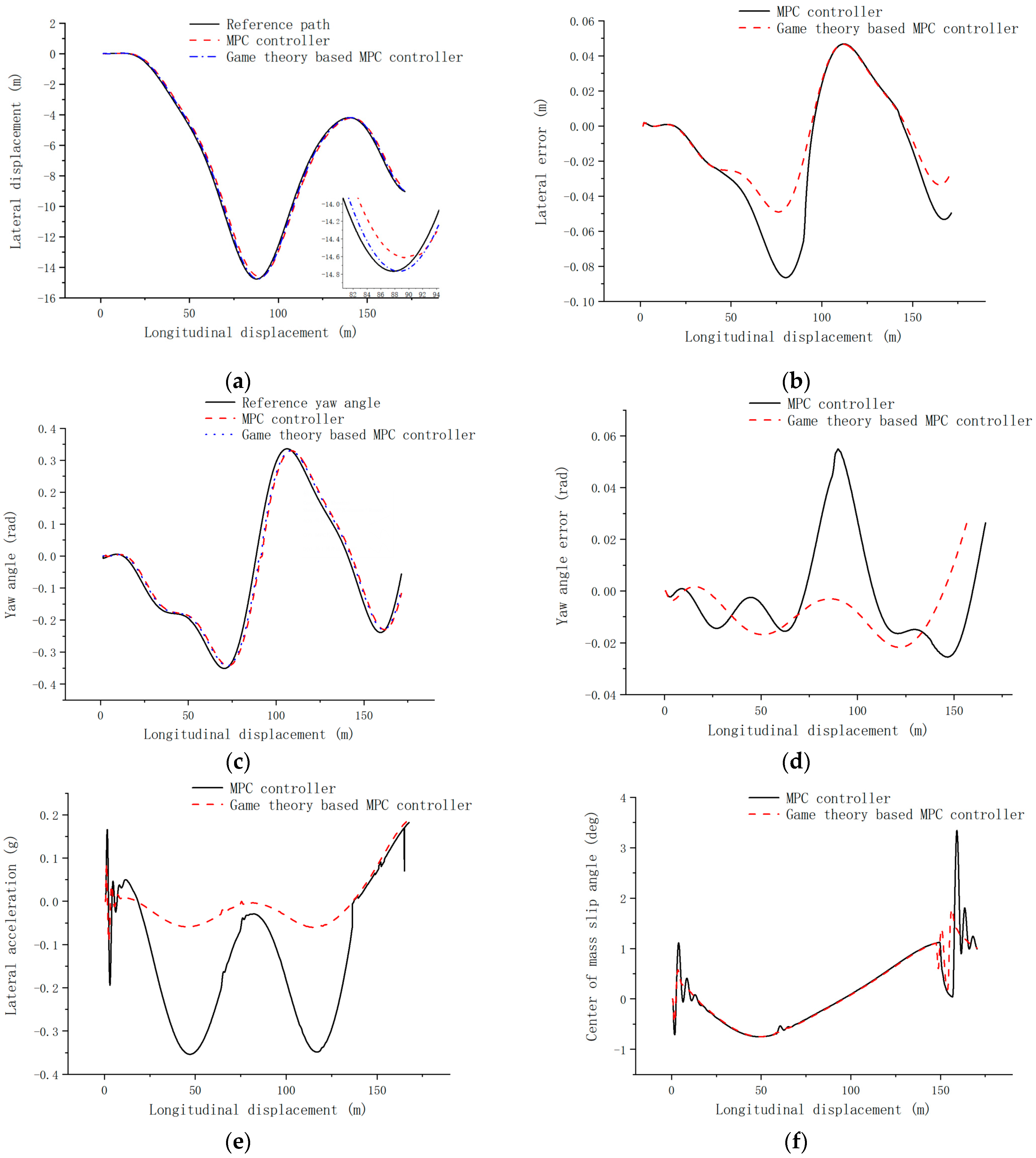
4.1. Low-Speed Road Simulation Verification

Set the reference path of the driverless electric formula racing car in MATLAB under high-speed following conditions, and the longitudinal speed to 30 km/h. A simulation comparison was made with an MPC controller and game theory based MPC controller applied to the driverless electric formula racing car, respectively, and the simulation results are shown in Figure 5.

The simulation results show that at a speed of 30 km/h, Figure 5a,c shows that both the MPC controller and the game theory based MPC controller work well in the whole tracking process. From Figure 5b it can be seen that the maximum lateral error of MPC controller the maximum lateral error is 0.08 m, while the maximum lateral error of the game theory based MPC controller is 0.04 m, which is 50% better than the MPC controller. From Figure 5d, it can be seen that the maximum yaw angle error of MPC controller is at 0.05 rad, while the maximum yaw angle error of the game theory based MPC controller is at 0.02 rad, which is 60% better than MPC controller. Figure 5e shows that the maximum lateral acceleration of the MPC controller is 0.36 g. The maximum lateral acceleration of the game theory based MPC controller is 0.2 g, which is 44% better than the MPC controller. Figure 5f shows that the maximum center of mass slip angle of MPC controller is 3.4 deg, and the maximum center of mass slip angle of game theory based MPC controller is 1.5 deg, which is 55% better than MPC controller, and the control effect of game theory based MPC controller is significantly better than MPC controller.

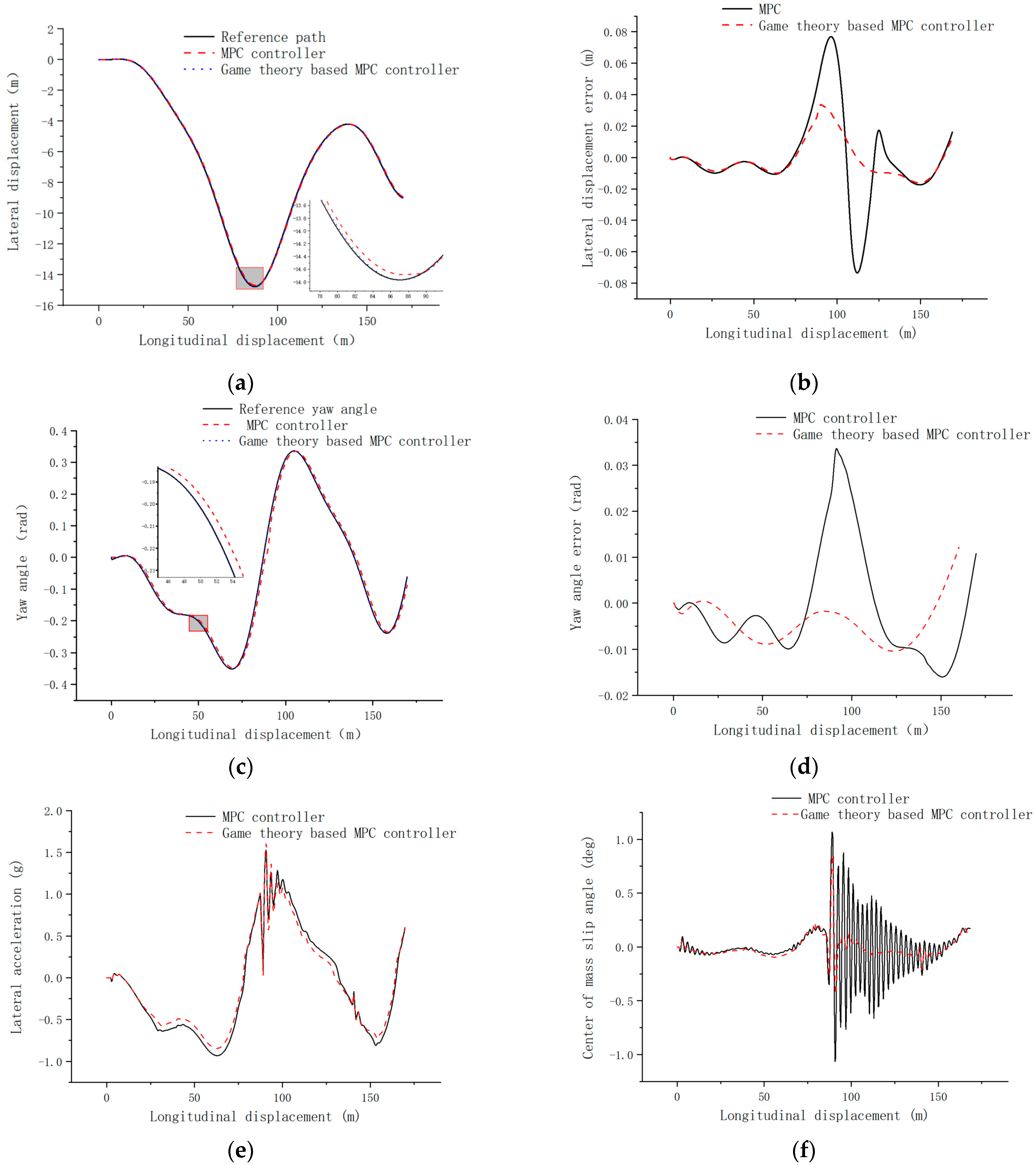
4.2. Medium-Speed Pavement Simulation Verification

Set the reference path of the driverless electric formula racing car in MATLAB under high-speed following conditions, and the longitudinal speed to 60 km/h. A simulation comparison was made with the MPC controller and game theory based MPC controller applied to the driverless formula racing car, respectively, and the simulation results are shown in Figure 6.

The simulation results show that at a speed of 60 km/h, Figure 6a,c shows that both the MPC controller and the game theory based MPC controller work well in the whole tracking process. From Figure 6b it can be seen that the maximum lateral error of MPC controller the maximum lateral error is 0.08 m, while the maximum lateral error of the game theory based MPC controller is 0.03 m, which is 62.5% better than the MPC controller. From Figure 6d, it can be seen that the maximum yaw angle error of MPC controller is at 0.03 rad, while the maximum yaw angle error of the game theory based MPC controller is at 0.012 rad, which is 60% better than MPC controller. Figure 6e shows that the maximum lateral acceleration of the MPC controller is 1.56 g. The maximum lateral acceleration of the game theory based MPC controller is 1.46 g, which is 6.4% better than the MPC controller. Figure 6f shows that the maximum center of mass slip angle of MPC controller is 1.07 deg, and the maximum center of mass slip angle of game theory based MPC controller is 0.83 deg, which is 22.4% better than MPC controller, and the control effect of the game theory based MPC controller is significantly better than MPC controller.

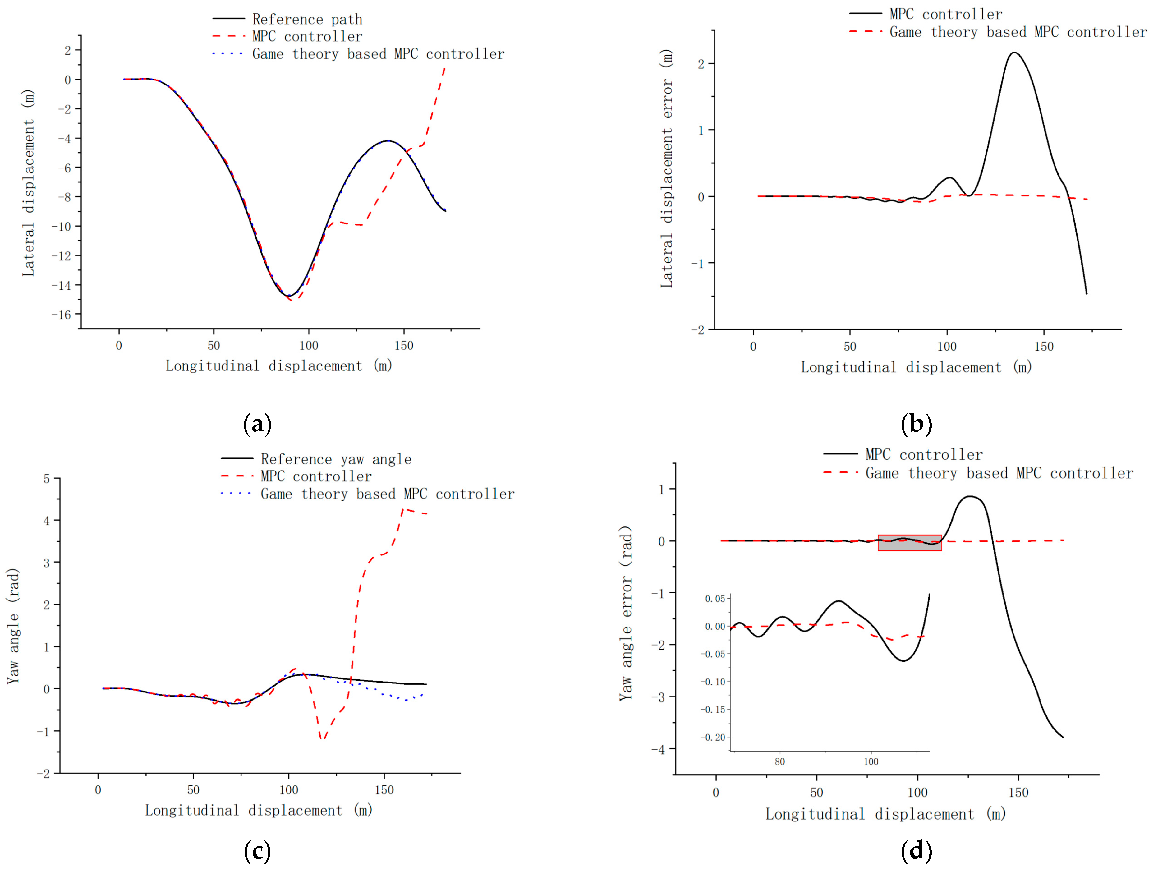
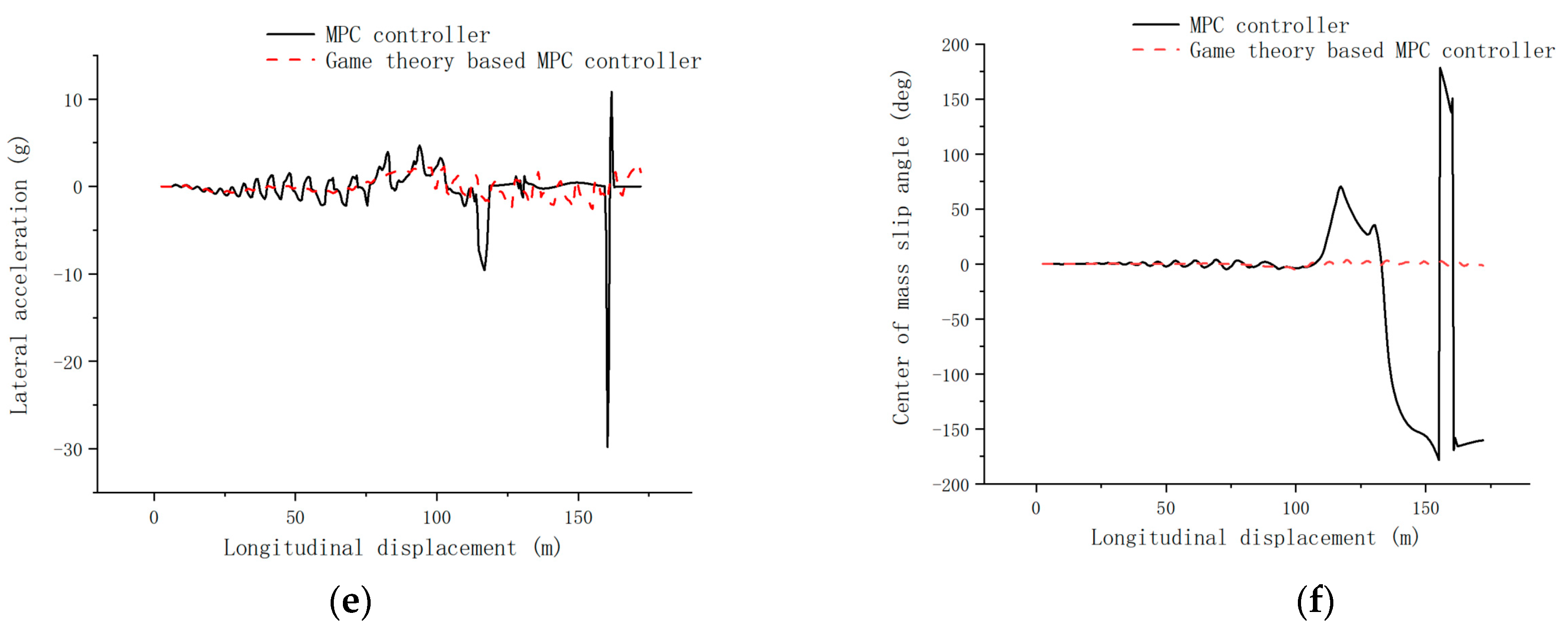
4.3. High-Speed Pavement Simulation Validation

Set the reference path of the driverless electric formula racing car in MATLAB under high-speed following conditions, and the longitudinal speed to 90 km/h. A simulation comparison was made with the MPC controller and the game theory based MPC controller applied to the driverless electric formula racing car, respectively, and the simulation results are shown in Figure 7.

The results show that, at a speed of 90 km/h, it can be seen from Figure 7a,c that during the whole tracking process, the MPC controlled lateral displacement and yaw angle suddenly changed when the longitudinal displacement was at 110 m. and the MPC controller based on game theory can performs well. From Figure 7b, it can be seen that the maximum lateral error of MPC controller is 2.2 m, while the maximum lateral error of the game theory based MPC controller is 0.1 m, which is 95% better than MPC controller. From Figure 7d, it can be seen that the maximum yaw angle error of MPC controller is at 0.85 rad, while the maximum yaw angle error of the game theory based MPC controller is at 0.03 rad, which is 96.4% better than MPC controller. Figure 7e shows that the maximum lateral acceleration of the MPC controller reaches 30 g, which is in a destabilized state, and the maximum lateral acceleration of the game theory based MPC controller is 2.6 g, which is 91.3% better than the MPC controller. Figure 7f shows that the maximum center of mass slip angle of the MPC controller is 179.8 deg, and the maximum center of mass slip angle of the game-theoretic-based MPC controller is 4.9 deg, which is 97.2% better than the MPC controller. The game theory based MPC controller is significantly better than the MPC controller. The MPC controller selects the weight matrix coefficients with better simulation results.

5. Conclusions

With the aim of addressing the dual-objective optimization problem of trajectory tracking accuracy and driving stability of driverless electric formula racing cars, a game theory-based trajectory tracking control study of driverless electric formula racing cars is conducted, and the following conclusions are drawn after theoretical research and experimental verification.

• Our proposed trajectory tracking control strategy based on game theory effectively coordinates the weight coefficients of trajectory tracking accuracy and driving stability, solves the dual-objective optimization problem, and improves the trajectory tracking accuracy and driving stability.
• Combining the model predictive control with game theory, the model predictive controller based on the evolutionary game of both players is designed, the lateral error is controlled within 0.1 m, and the transverse swing angle error is controlled within 0.5 rad under the high-speed tracing condition, which has a smaller change of control increment and better control effect compared with the single model predictive controller.
• The model prediction controller based on the evolutionary game of both sides has good trajectory tracking with strong robustness at high, medium, and low speeds.

References

1. Chen, Q.; Xie, Y.; Guo, S.; Bai, J.; Shu, Q. Sensing system of environmental perception technologies for driverless vehicle: A review of state of the art and challenges. Sens. Actuators Phys. 2021, 319, 112566. [Google Scholar] [CrossRef]
2. Nagai, M.; Mouri, H.; Raksincharoensak, P. Vehicle lane-tracking control with steering torque input. Veh. Syst. Dyn. 2002, 37 (Suppl. 1), 267–278. [Google Scholar] [CrossRef]
3. Fukushima, H.; Kim, T.H.; Sugie, T. Adaptive model predictive control for a class of constrained linear systems based on the comparison model. Automatica 2007, 43, 301–308. [Google Scholar] [CrossRef]
4. Zhao, F.; Wu, W.; Wu, Y.; Chen, Q.; Sun, Y.; Gong, J. Model Predictive Control of Soft Constraints for Autonomous Vehicle Major Lane-Changing Behavior With Time Variable Model. IEEE Access 2021, 9, 89514–89525. [Google Scholar] [CrossRef]
5. Taghavifar, H.; Rakheja, S. Path-tracking of autonomous vehicles using a novel adaptive robust exponential-like-sliding-mode fuzzy type-2 neural network controller. Mech. Syst. Signal Process. 2019, 130, 41–55. [Google Scholar] [CrossRef]
6. Ji, X.; Wang, J.; Zhao, Y.; Liu, Y.; Zang, L.; Li, B. Path Planning and Tracking for Vehicle Parallel Parking Based on Preview BP Neural Network PID Controller; Transactions of Tianjin University: Tianjin, China, 2015; Volume 21, pp. 199–208. [Google Scholar]
7. Kapania, N.R.; Gerdes, J.C. Design of a feedback feedforward steering controller for accurate path tracking and stability at the limits of handling. Veh. Syst. Dyn. 2015, 53, 1687–1704. [Google Scholar] [CrossRef] [Green Version]
8. Rosolia, U.; Bruyne, S.D.; Alleyne, A.G. Autonomous Vehicle Control: A Nonconvex Approach for Obstacle Avoidance. IEEE Trans. Control Syst. Technol. 2016, 25, 469–484. [Google Scholar] [CrossRef]
9. Mata, S.; Zubizarreta, A.; Pinto, C. Robust tube-based model predictive control for lateral path tracking. IEEE Trans. Intell. Veh. 2019, 4, 569–577. [Google Scholar] [CrossRef]
10. Ribeiro, A.M.; Fioravanti, A.R.; Moutinho, A.; de Paiva, E.C. Nonlinear state-feedback design for vehicle lateral control using sum-of-squares programming. Veh. Syst. Dyn. 2020, 60, 743–769. [Google Scholar] [CrossRef]
11. Ji, X.; He, X.; Lv, C.; Liu, Y.; Wu, J. Adaptive-neural-network-based robust lateral motion control for autonomous vehicle at driving limits. Control Eng. Pract. 2018, 76, 41–53. [Google Scholar] [CrossRef]
12. Bai, Y.; Li, G.; Jin, H.; Li, N. Research on Lateral and Longitudinal Coordinated Control of Distributed Driven Driverless Formula Racing Car under High-Speed Tracking Conditions. J. Adv. Transp. 2022, 2022, 7344044. [Google Scholar] [CrossRef]
13. Su, J.; Wu, J.; Cheng, P.; Chen, J. Autonomous Vehicle Control through the Dynamics and Controller Learning. IEEE Trans. Veh. Technol. 2018, 67, 5650–5657. [Google Scholar] [CrossRef]
14. Hu, Z.; Yu, Z.; Yang, Z.; Hu, Z.; Bian, Y. Rendering bounded error in adaptive robust path tracking control for autonomous vehicles. IET Control Theory Appl. 2022, 16, 1259–1270. [Google Scholar] [CrossRef]
15. Sun, Z.; Zou, J.; He, D.; Zhu, W. Path-tracking control for autonomous vehicles using double-hidden-layer output feedback neural network fast nonsingular terminal sliding mode. Neural Comput. Appl. 2022, 34, 5135–5150. [Google Scholar] [CrossRef]
16. Peicheng, S.; Li, L.; Ni, X.; Yang, A. Intelligent Vehicle Path Tracking Control Based on Improved MPC and Hybrid PID. IEEE Access 2022, 10, 94133–94144. [Google Scholar] [CrossRef]
17. Liang, Z.C.; Zhang, H.; Zhao, J.; Wang, Y.F. Trajectory Tracking Control of Unmanned Vehicles Based on Adaptive MPC. J. Northeast. Univ. Nat. Sci. 2020, 41, 835–840. [Google Scholar]
18. Xu, Y.; Tang, W.; Chen, B.; Qiu, L.; Yang, R. A model predictive control with preview-follower theory algorithm for trajectory tracking control in autonomous vehicles. Symmetry 2021, 13, 381. [Google Scholar] [CrossRef]
19. Bai, G.; Meng, Y.; Gu, Q. Path tracking control of vehicles based on variable prediction horizon and velocity. China Mech. Eng. 2020, 31, 1277–1284. [Google Scholar]
20. Zhang, K.; Sun, Q.; Shi, Y. Trajectory tracking control of autonomous ground vehicles using adaptive learning MPC. IEEE Trans. Neural Netw. Learn. Syst. 2021, 32, 5554–5564. [Google Scholar] [CrossRef]
21. Li, G.; Zhang, S.; Liu, L.; Zhang, X.; Yin, Y. Trajectory tracking control in real-time of dual-motor-driven driverless racing car based on optimal control theory and fuzzy logic method. Complexity 2021, 2021, 5549776. [Google Scholar] [CrossRef]
22. Ao, D.; Huang, W.; Wong, P.K.; Li, J. Robust backstepping super-twisting sliding mode control for autonomous vehicle path following. IEEE Access 2021, 9, 123165–123177. [Google Scholar] [CrossRef]
23. Geng, G.; Lu, S.; Duan, C.; Jiang, H.; Xiang, H. Design of autonomous vehicle trajectory tracking controller based on Neural Network Predictive Control. In Institution of Mechanical Engineers, Part D: Journal of Automobile Engineering; Sage: Thousand Oaks, CA, USA, 2023. [Google Scholar]
24. Jiao, H.-Y.; Li, Y.; Yang, L.-Y. An Improved Guide-Weight Method Without the Sensitivity Analysis. IEEE Access 2019, 7, 109208–109215. [Google Scholar] [CrossRef]
25. Shen, Y.; Hua, J.; Fan, W.; Liu, Y.; Yang, X.; Chen, L. Optimal design and dynamic performance analysis of a fractional-order electrical network-based vehicle mechatronic ISD suspension. Mech. Syst. Signal Process. 2023, 184, 109718. [Google Scholar] [CrossRef]
26. Wang, J.; Zhang, S.; Hu, X. A fault diagnosis method for lithium-ion battery packs using improved RBF neural network. Front. Energy Res. 2021, 9, 702139. [Google Scholar] [CrossRef]
27. Zhou, X.; Zhu, X.; Wu, W.; Xiang, Z.; Liu, Y.; Quan, L. Multi-objective Optimization Design of Variable-Saliency-Ratio PM Motor Considering Driving Cycles. IEEE Trans. Ind. Electron. 2021, 68, 6516–6526. [Google Scholar] [CrossRef]
28. Pacejka, H. Tire and Vehicle Dynamics; Elsevier: Oxford, UK, 2005. [Google Scholar]
29. Gong, J.; Jiang, Y.; Xu, W. Model Predictive Control for Self-Driving Vehicles; Beijing Institute of Technology Press: Beijing, China, 2014. [Google Scholar]
30. Zhang, J. Research on Models and Algorithms for Distributed Optimization Based on the Non-Cooperative Games; Zhejiang University: Hangzhou, China, 2014. [Google Scholar]
31. Pae, D.S.; Kim, G.H.; Kang, T.K.; Lim, M.T. Path planning based on obstacle-dependent gaussian model predictive control for autonomous driving. Appl. Sci. 2021, 11, 3703. [Google Scholar] [CrossRef]
32. Thomas, L.C. Games, Theory and Applications; Courier Corporation: North Chelmsford, MA, USA, 2012. [Google Scholar]
33. Sun, Q.W.; Lu, L.; Yan, G.L.; Che, H.A. Asymptotic stability of evolutionary equilibrium under imperfect knowledge. Syst. Eng. Theory Pract. 2003, 7, 11–16. [Google Scholar]
Figure 1. Game theory based on trajectory tracking control strategy.
Wevj 14 00084 g001
Figure 2. Sketch of vehicle dimensions.
Wevj 14 00084 g002
Figure 3. Three-degree-of-freedom dynamics model of vehicle.
Wevj 14 00084 g003
Figure 4. Evolutionary game stability strategy simulation.
Wevj 14 00084 g004
Figure 5. Simulation comparison of the two controllers at a speed of 30 km/h. (a) Comparative diagram of lateral displacement; (b) comparative diagram of lateral error; (c) comparative diagram of yaw; (d) comparative diagram of yaw angle error; (e) comparative diagram of lateral acceleration; (f) comparative diagram of center of mass slip angle.
Wevj 14 00084 g005
Figure 6. Simulation comparison of the two controllers at a speed of 60 km/h. (a) Comparative diagram of lateral displacement; (b) comparative diagram of lateral error; (c) comparative diagram of yaw; (d) comparative diagram of yaw angle error; (e) comparative diagram of lateral acceleration; (f) comparative diagram of center of mass slip angle.
Wevj 14 00084 g006
Figure 7. Simulation comparison of the two controllers at a speed of 90 km/h. (a) Comparative diagram of lateral displacement; (b) comparative diagram of lateral error; (c) comparative diagram of yaw; (d) comparative diagram of yaw angle error; (e) comparative diagram of lateral acceleration; (f) comparative diagram of center of mass slip angle.
Wevj 14 00084 g007aWevj 14 00084 g007b