An Energy Management Strategy for Hybrid Energy Storage System Based on Reinforcement Learning

Abstract

Due to the continuous high traction power impact on the energy storage medium, it is easy to cause many safety risks during the driving process, such as triggering the aging mechanism, causing rapid deterioration of the battery performance during the driving process and even triggering thermal runaway. Hybrid energy storage is an effective way to solve this problem. The ultracapacitor is an energy storage device that has high power density, which can withstand high instantaneous currents and can be charged and discharged quickly. By combining batteries and ultracapacitors in a hybrid energy storage system, energy sources with different characteristics can be combined to take advantage of their respective strengths and increase the efficiency and lifetime of the system. The energy management strategy plays an important role in the performance of hybrid energy storage systems. Traditional optimization algorithms have difficulty improving the flexibility and practicality of applications. In this paper, an energy management strategy based on reinforcement learning is proposed. The results indicate that the proposed reinforcement method can effectively distribute the charging and discharging conditions of the power supply and maintain the SOC of the battery and, at the same time, meet the power demand of working conditions at the cost of less energy loss and effectively realize the goal of optimizing the overall efficiency and effective energy management strategy.

1. Introduction

1.1. Research Background and Motivation

Global transportation is entering a transition to electrification and intelligence, and the transportation industry landscape is being reshaped. The shift from internal combustion engine driven to electric driven marks a major change in the future energy system in transportation. The energy density of the battery has a significant impact on the driving range of electric vehicles. The performance degradation and capacity decay of the battery seriously restrict the power capacity of the battery, and electric vehicles often encounter acceleration, climbing, emergency stops and other operation conditions that require high power charging or discharging of the battery. As a result, battery aging is accelerated, and reducing capacity degradation is a crucial aspect of energy storage technology [1]. There are many ways to extend the life of batteries, such as breakthroughs in materials and improvements in operating conditions. However, this paper mainly focuses on another perspective, which is from the view of system topology and control strategy.

Due to the continuous high traction power impact on the energy storage medium during the driving process, it is easy to trigger the aging mechanism and cause rapid deterioration of the battery performance, even triggering thermal runaway and other safety risks. Hybrid energy storage is an effective way to solve this problem [2]. For instance, a hybrid energy storage system composed of batteries and ultracapacitors can give full advantage of the high specific energy density of the battery and the high specific power density of the ultracapacitor, which not only ensures the power demand of the whole vehicle but also helps to lighten the energy system and comprehensively improves the reliability and economy of the energy storage system [3]. The extension of battery energy efficiency, lifetime health, economic management and optimal control techniques to multi-energy systems is a frontier scientific issue in the field of electrified transport and is of great research importance.

1.2. Literature Review

The power allocation and energy management strategy is the core of the hybrid energy storage system. Only a suitable power allocation and energy management strategy can bring the advantages of hybrid energy storage into full effect and achieve the desired goals. The purpose of designing a hybrid energy storage system control strategy is to improve the power output of the system and reduce the load on the lithium-ion battery, thus increasing the life of the lithium-ion battery and reducing system replacement costs [4]. Existing power allocation and energy management strategies fall into two main categories: rule-based control methods and optimization-based control methods.

Rule-based control methods include finite state machines [5] and logical threshold control [6], which are based on empirical intuition or some rough guidelines. Li et al. obtained a logical threshold control strategy by means of the pseudospectral method, which can obviously reduce the energy loss of the battery [7]. Peng et al. proposed a recalibration method to improve the performance of rule-based energy management through the results calculated by a dynamic programming algorithm. Then, an optimization-based rule development procedure is presented and further validated by hardware-in-loop simulation experiments. The simulation results show that the improved rule-based energy management strategy can reduce fuel consumption by 10.4% [8]. Hofman et al. combined the rule-based and equivalent consumption minimization strategy (RB-ECMS) to realize the energy management strategy of a hybrid energy vehicle. Compared with DP, RB-ECMS requires less calculation time to reach similar DP results within an accuracy of 1% [9]. Wang et al. focused on mode selection from different working conditions and power dividing modes and developed a rule-based control and balancing strategy [10]. Ramadan et al. developed a GPS/rule-based application of Petri nets that can provide energy management services both with and without GPS operation. The application references diverse driving circles and journeys. The results proved that the provided strategy reduces the fuel cost and has a more economic and simple structure [11]. These methods ignore the differences in the modes of the loads in different time slots and only design power allocation rules based on the overall statistical characteristics of the loads. The advantage of these methods is that they are easy and simple to use in real-time management, but the disadvantage is that they are too rigid and inflexible, and their performance cannot be guaranteed when they are in local load intervals that clearly do not match the overall characteristics of the system.

The optimization-based methods are a group of methods that design objective functions and use certain optimization methods to find the optimal values of the objective functions to derive the optimal energy management mode. Representative methods include dynamic programming [12,13], neural networks [14] and model predictive control [15]. Li et al. optimized the parameters through a multi-objective grey wolf optimizer and then used dynamic programming, a random forest algorithm and a support vector machine to realize both offline and online strategies [16]. Zhang et al. proposed a procedure to design an optimized power management strategy. The procedure includes a loss function involving the energy loss and the operation performance, a newly designed analysis method based on dynamic programming and adapting the optimizing frame [17]. Shen et al. described a framework that targets a multi-objective optimizing problem by minimizing the energy system and maximizing the battery circulating life and built an autonomy model. They also used a sample-based searching algorithm to optimize the model [18]. Serrao et al. compared three optimization-based methods, including dynamic programming, the Pontryagin minimum principle and the equivalent consumption minimization strategy. The real-time equivalent consumption minimization strategy achieves the best results with efficient performance [19]. Chen et al. built quadratic equations for the fuel rate and battery power. The problem is solved by using quadratic programming and the simulated annealing method together to find the optimal battery power commands and the engine-on power. In addition, the health of the battery is considered in the solution [20]. The advantage of these methods is that they can be oriented towards a specific load band to find the power allocation method with optimal performance. However, the disadvantage also comes from the fact that as the basis for obtaining the optimal method is a deterministic load segment, their power allocation methods have to be generated offline in advance and cannot be applied in online management situations. The optimality of the power allocation model is also not guaranteed if the load characteristics in actual use are significantly different from the predefined load segments.

1.3. Main Contributions

With the rapid development of artificial intelligence, intelligent strategies are gradually showing the advantages of flexibility and extensiveness, among which reinforcement learning algorithms stand out for their efficiency and lack of model dependency. Therefore, this article presents an energy management strategy based on reinforcement learning. The main contributions of this work are as follows: (1) The topology configuration based on actual working conditions was investigated and adopted. (2) A speed prediction algorithm based on the Markov chain is presented for better real-time energy management. The results indicated that accurate speed prediction can be obtained by the presented algorithm. (3) A power splitting algorithm based on Q-learning is proposed. Compared with the rule-based algorithm, the presented Q-learning has a high degree of robustness which can effectively distribute the charging and discharging conditions of the power supply and maintain the SOC of the battery and, at the same time, meet the power demand of working conditions at the cost of less energy loss and effectively realize the goal of optimizing the overall efficiency and effective energy management strategy.

1.4. Outline of the Article

The outline of the article is as follows: Section 2 provides the system model descriptions, including the structure of the hybrid energy storage system, the model of the vehicle and the models of the energy storage devices. Section 3 introduces the methodology of this work, which includes the speed prediction algorithm based on the Markov chain and the power splitting algorithm based on reinforcement learning. Section 4 presents the experimental results and discussions. Finally, the conclusions are presented in Section 5.

2. System Model Description

2.1. Structure of the Hybrid Energy Storage System

For the topology of the hybrid energy storage system, three kinds of structures are mainly considered: passive parallel topology, semi-active topology and fully active topology. The passive topology is simple and costs less, but the controllability is worse compared with the others, so it is difficult to apply in energy management strategies. Considering the cost and the energy loss of the bidirectional DC/DC converter and the controllability of the system, the semi-active topology was chosen. In the semi-active topology, the batteries and the ultracapacitors are connected by the DC/DC converter. Among the different types of semi-active topology, the battery/ultracapacitor topology designs the ultracapacitor to be connected with the DC bus directly. This kind of structure controls the states of the battery more conveniently, but the current of the DC bus will correspondingly become unstable. The structure adapted here is the battery/ultracapacitor topology, which is shown in Figure 1. In this kind of structure, the ultracapacitors are connected with the DC/DC converter, while the batteries are connected with the DC bus, which connects with the load through the DC/AC controller. The current of the structure tends to be stable for large currents and will influence the active life of the battery.

Once the topology of the system is defined, the structure can be configured according to the worldwide harmonized light vehicle test procedure (WLTP). The parameters of the battery and the ultracapacitor involved are presented in

Table 1. Parameters of the HESS.

Item	Parameter	Symbol	Value
Battery cell	Nominal voltage	UB,cell	3.2 V
	Stored energy	EB,cell	103 Wh
	Nominal capacity		30 Ah
	Nominal charge current		30 A
	Maximum discharge current		200 A
Ultracapacitor cell	Nominal voltage	Uc,cell	2.7 V
	Stored energy	EC,cell	3.04 Wh
	Nominal capacity	CC,cell	3000 F
HESS configuration	Series number of battery cells	NB,s	90
	Parallel number of battery cells	NB,p	2
	Series number of ultracapacitor cells	NC,s	122
	Parallel number of ultracapacitor cells	NC,p	4

. The energy storage should satisfy the nominal range of the vehicle. The energy requested in the nominal range E_range can be calculated as follows:

$$E_{\mathrm{range}}=E_{\mathrm{WLTP}}{S}_{\mathrm{range}}/S_{\mathrm{WLTP}}$$

(1)

where S_range denotes the WLTP nominal range, and S_WLTP denotes the actual range derived in the WLTP condition.

Thus, the total energy storage of the battery module should be no less than E_range. Additionally, the series voltage of the battery module should be no less than the DC link voltage. The following criteria are given:

$$E_{\mathrm{B},\mathrm{s}}{E}_{\mathrm{B},\mathrm{p}}{E}_{\mathrm{B},\mathrm{cell}}-E_{\mathrm{Br},\mathrm{cell}}\ge E_{\mathrm{range}}$$

(2)

$$N_{\mathrm{B},\mathrm{s}}{U}_{\mathrm{B},\mathrm{cell}}\ge U_{\mathrm{B},\mathrm{DC}}$$

(3)

where E_Br,cell denotes the extra energy waste per cell from the mass increase of the battery module. According to our assessment, when the mass of the battery module increases by 72 g (the mass of one battery cell), it will require approximately 0.07 Wh additional energy, which is almost 1% of the energy storage of a battery cell.

The ultracapacitor module should meet the peak power demand first and be large enough to store regenerative energy every time the load power is positive. The maximum energy demand can be calculated as follows:

$$E_{\mathrm{peak}}=\underset{i}{\max }{\displaystyle \underset{t_{\mathrm{p},i}}{\int }\left|P_{\mathrm{WLTP}}\left(t\right)-P_{\mathrm{B},\mathrm{n}}\right|dt}$$

(4)

where P_B,n denotes the nominal power of the battery, and t_p,i denotes the ith continuous period when P_WLTP is larger than P_B,n.

Similarly, the maximum energy demand of the regenerative period is defined as follows:

$$E_{\mathrm{regn}}=\max {\displaystyle \underset{t_{\mathrm{p},i}}{\int }\left|P_{\mathrm{WLTP}}\left(t\right)\right|dt}$$

(5)

where t_r,i denotes the ith continuous period when P_WLTP is positive.

According to the voltage demand of the DC bus, the following criteria are needed:

$$\frac{3}{4}{N}_{\mathrm{C},\mathrm{s}}{N}_{\mathrm{C},\mathrm{p}}{E}_{\mathrm{C},\mathrm{cell}}\ge \underset{}{\max }\left(E_{\mathrm{regn}},E_{\mathrm{peak}}\right)$$

(6)

$$\frac{1}{2}{U}_{\mathrm{C}}<U_{\mathrm{B},\mathrm{s}}{U}_{\mathrm{B},\mathrm{cell}}<U_{\mathrm{C}}$$

(7)

where the voltage of the ultracapacitor should be in the period of (1/2 ultracapacitor, ultracapacitor) to ensure that the DC/DC converter is working in an efficient state.

With the analysis above, we calculated the appropriate configuration of the hybrid energy system. The results are shown in Table 1.

2.2. Model Description

2.2.1. Vehicle Power Model

The real-time power demand is calculated as follows [16]:

$$P_{\mathrm{re}}=\left(\mu Mgcos\theta +Mgsin\theta +0.5\mathrm{A}{\rho }_{\mathrm{air}}{C}_{\mathrm{air}}{v}^2+{\delta }_{\mathrm{c}}Ma\right)v$$

(8)

where μ denotes the rolling resistance coefficient, g denotes the gravitational acceleration, M denotes the vehicle mass, A denotes the vehicle windward area, θ is the longitudinal road gradient, ρ_air denotes the air density, C_air denotes the air resistance coefficient, v is the velocity, a is the acceleration, and δ_c is the rotation mass correction coefficient. The values of the parameters above are listed in

Table 2. Parameters of the vehicle.

Parameter	Symbol	Value
Vehicle mass	M	1360 kg
Rolling resistance coefficient	μ	0.0015
Gravitational acceleration	g	9.8 m/s2
Longitudinal road gradient	θ	0
Air density	ρair	1.202 kg/m3
Vehicle windward area	A	2 m3
Rotation mass correction coefficient	δc	1.04
Air resistance coefficient	Cair	0.3
Power transmission system efficiency	ηs	0.9
WLTP nominal range	Srange	150 km
Battery module voltage	UB,DC	>400 V

. It should be noted that the circumstances of actual driving are complex so it is impossible to consider the influence of the road gradient, so we assume the longitudinal road gradient is zero.

The electric drive power P_e is formulated as Equation (9):

$$P_{\mathrm{e}}=\left\{\begin{array}{c}{P}_{\mathrm{re}}/{\eta }_{\mathrm{s}}, P_{\mathrm{re}}\ge 0\\ {\eta }_{\mathrm{s}}{P}_{\mathrm{re}}, P_{\mathrm{re}}<0\end{array}\right.$$

(9)

where η_s denotes the efficiency of the power transmission system; when P_re is positive, the vehicle is in traction mode, and when P_re is negative, the vehicle is in regenerative braking mode.

2.2.2. Battery Model

A lithium-ion battery is a kind of nonlinear electrochemical device containing a series of complex physical and chemical processes, and it is very difficult to accurately model it. We have considered more accurate model-like nonlinear models in recent research [21], but the accuracy brings complexity. The key point of the paper is the HESS based on RL, so we tend to use more simple models.

Considering the complexity and accuracy requirements of the model, this study uses the Thevenin model to model lithium-ion batteries [22]. Figure 2a is the Thevenin-equivalent circuit model of the battery, which mainly includes an open voltage source, an ohmic internal resistance and a parallel RC network. The open-circuit voltage source can be used to describe the steady-state characteristics of the battery, while the ohmic internal resistance and parallel RC network can be used to describe the transient characteristics of the battery. The model considers the transient and steady characteristics of the battery at the same time, and its accuracy and computational complexity are moderate, so this model is appropriate for simulation.

Based on the Thevenin model of the battery, the following expressions can be obtained:

$$U_b=U_{ocv}-U_o-U_p$$

(10)

$$I_b=-U_o/R_o=-U_p/R_p-C_{p}d{U}_p/dt$$

(11)

where U_b is the terminal voltage of the battery, U_ocv is the open circuit voltage of the circuit, U_o is the voltage drop of the ohmic internal resistance, I_b is the charging current, R_o is the ohmic internal resistance, and R_p and C_p are the polarization internal resistance and polarization capacitance of the battery, respectively.

The open-circuit voltage U_ocv in the formula can be obtained from the curve table of OCV-SOC through experiments and then from the electrochemical model. Taking the combined model as an example, the OCV of the battery can be written as:

$$U_{ocv}=k_0+k_{1}SO{C}^2+k_{2}SOC+k_3/SOC+k_4\log \left(SOC\right)+k_5\log \left(1-SOC\right)$$

(12)

where $k_0$ to $k_5$ are the model coefficients.

2.2.3. Ultracapacitor Model

As shown in Figure 2b, the standard RC model of the ultracapacitor is adopted in this study, which consists of an ideal capacitor C_u and an equivalent series resistance R_u [22]. This model can accurately reflect the external electrical characteristics of the ultracapacitor during charging and discharging. By analyzing this circuit, the following expressions can be obtained:

$$U_u=R_u{I}_u+U_c$$

(13)

$$d{U}_c/dt=I_u/C_u$$

(14)

where U_u is the terminal voltage of the ultracapacitor, U_c is the voltage across the equivalent series resistor, I_u is the charging current, and C_u and R_u are the ideal capacitor and the equivalent series capacitor, respectively.

3. Methodology

3.1. Speed Prediction Based on Markov Chain

To apply the energy management strategy in some real-time calculations, accurate speed prediction is needed. The method employed in the speed prediction in this research is the Markov Chain. According to the operation condition of the WLTP, the velocity and the acceleration were divided into limited states:

$$a\in \left\{a^1,a^2,\dots a^{N_a}\right\}$$

(15)

$$v\in \left\{v^1,v^2,\dots v^{N_v}\right\}$$

(16)

where N_a is the number of acceleration states, and N_v is the number of velocity states. According to the data in the WLTP, the range of the acceleration is −1.5–1.7 $\mathrm{m}/{\mathrm{s}}^2$, and then the acceleration is separated with a gap of 0.1 $\mathrm{m}/{\mathrm{s}}^2$. The range of velocity is 0–36.5 $\mathrm{m}/\mathrm{s}$, and then the velocity is separated with a gap of 0.5 $\mathrm{m}/\mathrm{s}$.

Next, the velocity and acceleration of each moment were reflected into the quantities of states $v^l\mathrm{and}{a}^i$, and then the acceleration during n moments in the future was recorded, which will be reflected into the quantities of states where n denotes the length of prediction. Thus, the state transition probability can be defined:

$$P_{il,j}^n=P_r\{a_{k+n}=a^j|a_k=a^i,v_k=v^l\}$$

(17)

The number of times the acceleration transmits is counted from $a^i$ to $a^j$ in n steps when the velocity is exactly $v^l$, which is supposed to be $m_{il,j}^n$. $m_{il}^n$ denotes the number of times the acceleration transmits from $a^i$ to all acceleration states in n steps when the velocity is $v^l$. We have:

$$P_{il,j}^n=m_{il,j}^n/m_{il}^n$$

(18)

When the velocity is $v^l$, all the transition probabilities in n steps form the state transition probability matrix $P_l^n$:

$$P_l^n=\left[\begin{array}{ccc}{P}_{1l,1}^n& \cdots & P_{1l,N_a}^n\\ ⋮& \ddots & ⋮\\ P_{N_{a}l,1}^n& \cdots & P_{N_{a}l,N_a}^n\end{array}\right]$$

(19)

From the matrix above, the velocities in n steps in the future can be predicted: (1) reflect the actual velocity and acceleration to the state quantity $v^l\mathrm{and}{a}^i$ at the current moment; (2) calculate the expectation of acceleration after n steps based on the state transition probability matrix; and (3) according to the expectation of acceleration above, calculate the acceleration in m steps ($1\le m\le n$).

3.2. Power Splitting Based on Reinforcement Learning

3.2.1. Basic Concepts

In this section, the Q-learning algorithm is adopted to optimize the overall efficiency and obtain an effective energy management strategy for the WLTP. A series of basic concepts of reinforcement learning need to be introduced hierarchically to define the Q-learning algorithm.

Reinforcement learning solves and improves the control performance of Markov decision problems. Its main architecture revolves around a so-called learning agent, which has access to sensing the environment state and taking actions that conversely affect the controlled environment. To improve control performance, a reward signal is defined that can guide the agent to achieve higher cumulative values through a trial-and-error mechanism. Reinforcement learning can be divided into two categories: model-based learning and model-free learning. In model-based learning, considering the multi-step reinforcement learning task, the machine has modeled the environment, which can simulate the same or similar situation with the environment inside the machine. Regarding model-free learning, in a realistic reinforcement learning task, it is often difficult to know the transition probability and reward function of the environment or even how many states there are in the environment. If the learning algorithm does not depend on environment modeling, it is called model-free learning, which is much more difficult than model-based learning.

The biggest advantage of model-based learning is that agents can plan in advance, try possible future choices in advance when they go to each step, and then clearly choose from these candidates. The biggest disadvantage is that agents often cannot get the real model of the environment. If the agent wants to use the model in a scene, it must learn completely from experience, which will bring many challenges. The biggest challenge is that there is an error between the model explored by the agent and the real model, which will cause the agent to perform well in the learning model but not well in the real environment. In order to obtain an energy management strategy that can cope with the real environment well, the model-free learning method is used here. There are two kinds of methods in model-free reinforcement learning: the Monte-Carlo update and temporal-difference update. In actual working conditions, the required power is changing every second. According to this characteristic, Q-learning is selected to explore energy management. At the same time, the rule-based method is used to provide another integrated energy management system and be compared with Q-learning to verify its effectiveness.

3.2.2. Power Splitting Based on Q-Learning

Q-learning was proposed for solving Markov decision problems. As one of the most popular off-policy RL methods, Q-learning is expected to maximize the total reward $\sum R$. Consequently, the optimal value function that guides the decision process of the policy can be defined as the distribution over the given current state S(t) and control action A(t).

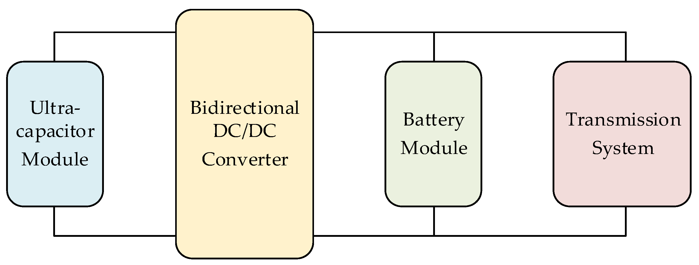
In the integrated energy management system, there are three kinds of changing states: the SOC representing the battery state, state-of-voltage (SOV) representing the capacitor state, and P_dem representing system output. The constraints of the state variable S(t) = {SOC(t), SOV(t), P_dem(t)} can be defined as:

$$\left\{\begin{array}{l}0.4\le SOC\left(t\right)\le 0.9\\ 0.2\le SOV\left(t\right)\le 0.9\\ -40\le P_{dem}\left(t\right)\le 40\end{array}\right.$$

(20)

where P_dem is the required power (unit: kW).

The constraints of the control variable A(t) = {I_c(t), I_v(t)} are defined as:

$$\left\{\begin{array}{l}20\le \left|I_c\left(t\right)\right|\le 40\\ 20\le I_v\left(t\right)\le 40\end{array}\right.$$

(21)

where I_c is the battery current, and I_v is the ultracapacitor current (unit: A).

The reward function is:

$$R=\left\{\eta + \gamma \left|\Delta SOC\right|\right\}$$

(22)

where $\eta$ is a variable; with the size of the total loss value under each second working condition, it is randomly selected in the corresponding interval. When the total loss is less than the required power of 20%,$\gamma$ is 1; otherwise, $\gamma$ is −1.$△SOC$ = $SOC$ − $SO{C}_{pre}$, is used to limit the SOC range of battery packs.

R_t is the reward at a single time step t; for estimating the long-term return, the return G_t is used to represent the cumulative value of reward R_t after time t, and its recursion form is:

$$G(t)={\displaystyle \sum }_{k=0}^{\infty }{\gamma }^{k}R(t+k)=R(t)+\gamma (R(t+1)+\gamma R(t+2)+\dots )=R+\gamma G(t+1)$$

(23)

where γ∈(0,1) is the discount factor.

Strategy b is a mapping from the state to the likelihood of selecting each action. The state value function v_b(s) is defined as the expected return starting from state s and following strategy b, expressed as:

$$v_b=E_b[G(t)|S(t)=s]$$

(24)

where S(t) is the state at time t.

Meanwhile, the action value function q_b(s, a) is also defined as the expected return starting from state s, taking action a and following strategy b:

$$q_t\left(s,a\right)={\mathrm{E}}_{\mathrm{b}}[G(t)|S(t)=s,A(t)=a]$$

(25)

where A(t) is the action at time t. Then, again, the recursive form can be derived:

$$q_t\left(s,a\right)==R(t){\displaystyle \sum _{s(t+1)\in S}p\left(s(t+1)|s(t),a(t)\right)}{\displaystyle \sum _{a(t+1)\in A}b\left(a(t+1)|s(t+1)\right)q_b\left(s(t+1),a(t+1)\right)}$$

(26)

where s(t) and s(t + 1) represent specific states at time t, and t + 1. a(t) and a(t + 1) represent the specific actions at time t and t + 1.

The optimal action value function q*(s, a) is defined as the maximum action value function in all strategies, and its recursive form can be expressed as:

$$q\ast \left(s(t),a(t)\right)=R(t)+{\displaystyle \sum _{s_{t+1}\in \mathrm{S}}p\left(s(t+1)|s(t),a(t)\right){\max }_{a(t+1)}q\ast \left(s(t+1),a(t+1)\right)}$$

(27)

If q*(s, a) is known, the optimal strategy b* can be obtained by maximizing q*(s, a).

As the real value of the optimal action value function is difficult to obtain, the estimated value of q*(S(t), A(t)) − Q(S(t), A(t)) is used. In a sequential difference method including Q-learning, the difference between the estimated value Q(S(t), A(t)) and the better estimated value R(t) + γQ(S(t), A(t)) is used to update Q(S(t), A(t)):

$$Q(S\left(t\right),A\left(t\right))=Q(S\left(t\right),A\left(t\right))+\alpha (R\left(t\right)+\gamma Q(S\left(t+1\right),A\left(t+1\right))-Q(S\left(t\right),A\left(t\right)))$$

(28)

where α is the learning rate.

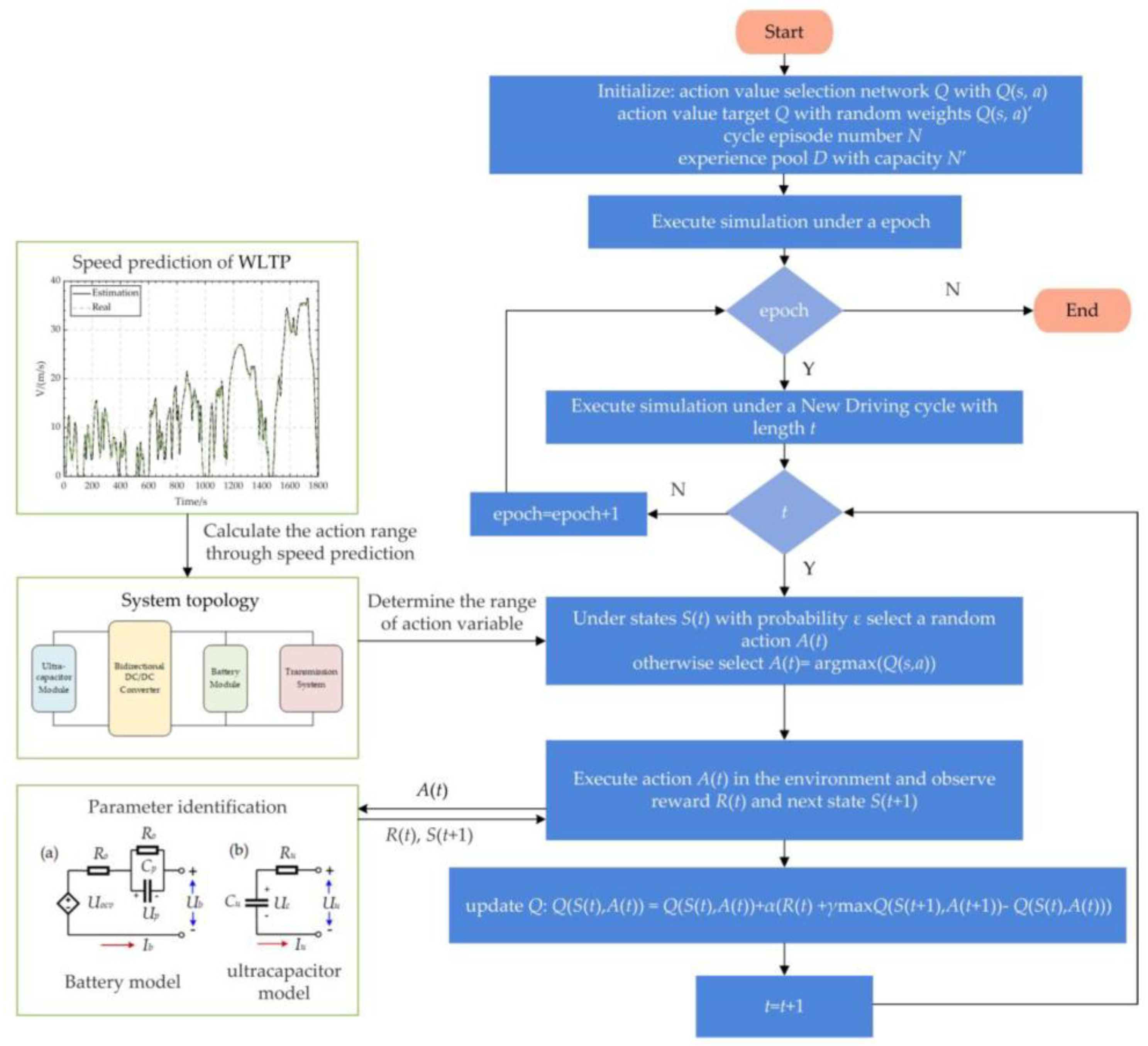
The algorithm block diagram is shown in Figure 3, which demonstrates the basic method of the algorithm, including the usage of previous work. The exact procedures of the QL algorithm in this article are shown in Algorithm 1.

Algorithm 1: Q-Learning

Initialization of Q-learning: Determine algorithm parameter boundary: α∈(0,1), γ∈(0,1), numbers of episodes N, working condition duration T, initialize action value target Q with random weights Q(s, a)’ and experience pool D with capacity N for episode = 1: N do  for t = 1:T do    With probability π select a random action A(t)    Otherwise, select A(t) = arg maxQ(S(t), A(t))     execute action A(t) and observe reward R(t) and next state S(t + 1)     update Q follows: Q(S(t), A(t)) = Q(S(t), A(t)) + α[R(t) + γmaxQ(S(t + 1), a) − Q(S(t), A(t))]     update S(t) and A(t)  end for end for

4. Results and Discussion

4.1. Model Verification

First, at 25 °C, the open-circuit voltage of the battery under different SOCs was measured. After fitting with Equation (12), the lithium-ion battery model can be identified according to the RLS algorithm. The voltage prediction result is shown in Figure 4a, and the error between the voltage prediction result and the actual voltage is shown in Figure 4b. The polynomial fitting values of the ohmic resistance, polarization capacitance and polarization internal resistance with respect to the SOC are shown in

Table 3. Battery parameter fitting.

SOC	${\mathit{R}}_{\mathit{o}}/\Omega$	${\mathit{C}}_{\mathit{p}}$$/\times {10}^4 \mathrm{F}$	${\mathit{R}}_{\mathit{p}}/\Omega$
0.1	0.0014	3.2301	0.0042
0.2	0.0013	3.2723	0.0043
0.3	0.0012	3.4376	0.0045
0.4	0.0013	3.8351	0.0047
0.5	0.0011	3.7726	0.0050
0.6	0.0012	4.2605	0.0053
0.7	0.0011	4.8798	0.0063
0.8	0.0012	5.0248	0.0078
0.9	0.0015	4.9906	0.0109

. Generally, the voltage curve predicted by the recursive least square method is almost consistent with the actual measured curve, and the root mean square error of the voltage is 0.0015 V, which meets the requirements of model accuracy.

In addition, it can be found that the error between the voltage prediction result and the real value is obviously larger at the beginning of the experiment (the SOC is close to 1) and before the end of the working condition (the SOC is close to 0). This is because there are two logarithmic functions in Equation (12) of the combined model. When $soc$ is close to 1 or 0, the logarithmic functions quickly approach infinity, so there is a large error. On the other hand, when the SOC is close to 1 or 0, “overcharge” and “overdischarge” will affect the performance and life of the battery. Considering the large error when the SOC is close to 1 or 0 and the possible problems of “overcharge” and “overdischarge”, we should try our best to make the battery work in SOC∈(0.1, 0.9) when modeling and experimenting.

Through the RLS algorithm, the ultracapacitor model can be identified similarly to the battery model, and the voltage prediction results and errors are shown in Figure 4c,d. As the model of the supercapacitor is simple, the error of voltage prediction of the RLS algorithm after convergence is very small, which meets the modeling requirements. The identification values of C_u and R_u of the ultracapacitor can be regarded as fixed values, as shown in

Table 4. Parameter identification of the ultracapacitor.

Model Parameter	Parameter Identification Result
Ideal capacitance	3053.3 F
Equivalent series resistance	0.0037 Ω

.

4.2. Speed Prediction Results

The speed prediction results and prediction error are plotted in Figure 5a,b, from which we can infer that the speed prediction based on the Markov chain is an accurate approach with WLTP working conditions.

4.3. Power Splitting Results

In this section, to study the effectiveness of the QL method, the results are compared with the rule-based strategy, and standard WLTP working conditions were used for simulation verification.

Figure 6a,b show the power allocation based on the rule strategy and reinforcement learning, respectively. Under WLTP conditions, the power allocation of the two strategies can fully meet the power demand by the battery when the power demand is low and meet the demand by the battery output power with a small amount when the power demand is high. Compared with the traditional pure battery drive, both strategies greatly save battery energy.

Figure 7a shows the comparison of power allocation between the rule-based strategy and reinforcement learning strategy. To protect the battery, according to the specific working conditions, when the outside world needs power from the power supply system, the current output by the battery is limited from 20 to 40 A, and the current input when the battery is charged is limited from −40 to −20 A. This choice can keep the input and output power of the battery in a stable range, making the power output more stable, thus protecting the battery and prolonging the battery life.

Obviously, compared with the rule-based approach, the work points in the learning-based strategy are not only more concentrated but also more located in the low fuel consumption zone, thus achieving a more reasonable distribution. At the same time, in terms of energy management, we can see that compared with the rule-based method, when the power supply system needs to output power, the reinforcement learning method does not always choose the battery output power but appropriately increases the output power of the capacitor according to the size of the output energy required by the power supply system to meet the power demand and charge the battery. This energy management mode breaks through the rule-based charging and discharging modes and provides a brand-new energy management idea.

Figure 7b shows the SOC trajectory comparison between rule-based and reinforcement learning. Compared with the rule-based method, the reinforcement learning method chooses working power. The SOC value in a period of time does not change much compared with the average SOC value, and the final SOC value of reinforcement learning is higher than that of the rule-based method. Compared with the rule-based method, the reinforcement learning method can better maintain the SOC. Compared with the rule-based method, the energy management method obtained by reinforcement learning can make full use of the advantages of ultracapacitors in the composite power supply system when the power demand (e.g., from 600 to 1200 s) is large and changes rapidly and effectively maintain the SOC of the battery while providing the system power demand, thus prolonging the service life of the battery. This result verifies the effectiveness of reinforcement learning in delaying battery use.

Table 5. Efficiency comparison.

Strategy	Comprehensive Efficiency
Reinforcement learning	0.3096
Rule-based	0.2096
Pure cell	0.1016

shows the comparison of comprehensive efficiency. It is calculated by dividing the total energy required under the WLTP condition by the total energy output of the battery. Compared with the rule-based strategy, the strategy based on reinforcement learning can fully meet the power demand and greatly improve the comprehensive efficiency. This result verifies the effectiveness of the energy management strategy of reinforcement learning in energy saving. Combined with the previous results, it can be seen that in facing the complex, nonlinear and dynamic WLTP working condition, the proposed reinforcement method can effectively distribute the charging and discharging conditions of power supply and maintain the SOC of battery and, at the same time, meet the power demand of working conditions at the cost of less energy loss and effectively realize the goal of optimizing the overall efficiency and effective energy management strategy.

5. Conclusions

The energy management strategy is significant for hybrid energy storage systems. Traditional optimization algorithms have difficulty improving the flexibility and practicality of applications. In this paper, an energy management strategy based on reinforcement learning is proposed. Moreover, the speed prediction algorithm based on the Markov chain is employed for better real-time energy management. The results indicated that accurate speed prediction can be obtained by the presented algorithm. The power splitting algorithm based on Q-learning is proposed, and the results showed that the proposed reinforcement method can effectively distribute the charging and discharging conditions of the power supply and maintain the SOC of the battery and, at the same time, meet the power demand of working conditions at the cost of less energy loss and effectively realize the goal of optimizing the overall efficiency and effective energy management strategy. Future work will focus on improving the efficiency and application of reinforcement learning algorithms.