Enhancing IoT Device Security through Network Attack Data Analysis Using Machine Learning Algorithms

Abstract

The Internet of Things (IoT) shares the idea of an autonomous system responsible for transforming physical computational devices into smart ones. Contrarily, storing and operating information and maintaining its confidentiality and security is a concerning issue in the IoT. Throughout the whole operational process, considering transparency in its privacy, data protection, and disaster recovery, it needs state-of-the-art systems and methods to tackle the evolving environment. This research aims to improve the security of IoT devices by investigating the likelihood of network attacks utilizing ordinary device network data and attack network data acquired from similar statistics. To achieve this, IoT devices dedicated to smart healthcare systems were utilized, and botnet attacks were conducted on them for data generation. The collected data were then analyzed using statistical measures, such as the Pearson coefficient and entropy, to extract relevant features. Machine learning algorithms were implemented to categorize normal and attack traffic with data preprocessing techniques to increase accuracy. One of the most popular datasets, known as BoT-IoT, was cross-evaluated with the generated dataset for authentication of the generated dataset. The research provides insight into the architecture of IoT devices, the behavior of normal and attack networks on these devices, and the prospects of machine learning approaches to improve IoT device security. Overall, the study adds to the growing body of knowledge on IoT device security and emphasizes the significance of adopting sophisticated strategies for detecting and mitigating network attacks.

1. Introduction

IoT devices represent a paradigm shift in the way we interact digitally with the physical world, as it enables the connectivity and communication between a vast array of devices and systems through a communication network. These interconnected devices, which can range from simple sensors to complex machinery, are equipped with the ability to gather, process, and transmit data, allowing them to sense and respond to their surroundings in an autonomous manner. The IoT shares the idea of an autonomous system responsible for transforming physical computational devices into smart ones in an activity-generated environment under existing networks through embedded systems. Embedded systems provide the essential combination of hardware and firmware, along with Internet access, to execute respective tasks [1]. The key features of IoT devices comprise their abilities of actuation, processing, connectivity, and data storage. Contrarily, storing and operating information while maintaining its confidentiality and security throughout the whole operation process considering transparency in its privacy, data protection, and disaster recovery, is a concerning issue in the IoT. This talks about the vulnerabilities such as open telnet ports, which are devastating considering conditions such as outdated Linux firmware, communications of data without encryption, etc., being common in the IoT ecosystem, keeping it vulnerable to attacks such as a botnet, etc. [2]. To prevent this situation, research on false network detection respective to the concept of machine learning (ML) for tracking any irregular traffic in the IoT ecosystem needs to be prioritized, as the detection mainly deals with the behavior of those communications from the devices to the routers and switches through the existing network, and any irregular behavior can be traced down and operated on. IoT devices have become increasingly popular in recent years due to their ability to connect to the Internet and facilitate remote communication and control. However, the proliferation of these devices has also led to a rise in security breaches and attacks, particularly through the use of botnets [3]. Botnets are networks of compromised devices that are controlled remotely by a malicious actor. These devices can be utilized to initiate distributed denial of service (DDoS) attacks, send spam emails, or steal sensitive information. IoT devices, which often have weak security measures and are not regularly patched or updated, are particularly vulnerable to compromise and can be easily recruited into a botnet [4]. One example of a significant IoT-based botnet attack was the Mirai botnet, which was first identified in 2016. This botnet was responsible for several high-profile DDoS attacks, including an attack on the Krebs on Security website and an attack on the Dyn DNS provider, which disrupted Internet service for much of the Eastern United States. The Mirai botnet compromised many IoT devices, including routers, security cameras, and digital video recorders, by using a list of default or commonly used passwords to gain access.

Other research has highlighted the security risks associated with IoT device interoperability and the use of third-party libraries. In a paper published in 2019, researchers found that the use of third-party libraries in IoT devices can lead to vulnerabilities that attackers can exploit. Additionally, the lack of standardization and security measures in developing IoT devices can lead to interoperability issues that attackers can exploit [5]. The ability to detect abnormal changes in a system’s information, variables, or subsystems and identify it as a deviation from normal behavior is possible by thoroughly understanding the ecosystem and recognizing such changes based on prior experience. This concept can also be adapted to detecting normal and abnormal network traffic. Data traffic from IoT devices has been found to be distinct; it often exchanges data with fixed sets of endpoints rather than a vast diversity in penetration of its web servers, which helps to track the regular traffic and disobey the attack traffic according to the behavior and penetration change. IoT devices also have distinct states, so the behavior can be conveniently differentiated [6]. Traditional security methods that only react after an attack has been detected may not be sufficient to protect the network. To prevent these attacks from affecting the network’s performance, a system that deploys smart and state-of-the-art security measures is necessary for IoT networks. Using proactive security methods can mitigate potential security weaknesses in the network. These security measures should also not cause any delays in the network, as IoT networks require low latency. To meet these requirements, AI and ML approaches can be used to provide the necessary intelligence to create smart security systems. AI and ML algorithms are able to analyze large amounts of data and identify common patterns that indicate an intrusion. Datasets are important for the effective use of intrusion-based security systems. Without a dataset that resembles the network flows in the IoT, it is difficult to validate the effectiveness of AI-based security measures. As IoT networks become increasingly important, having a dataset that can be used for this purpose will be a valuable contribution. By 2025, it is anticipated that the global market for IoT end-user solutions will reach approximately $1.6 trillion, posing a new growing danger from exposed telnet ports, out-of-date Linux firmware, and numerous other related vulnerabilities [7]. The expansion of these insecure IoT devices opens up wide varieties of new cybersecurity attack factors, most notably IoT Botnet attacks. IoT botnet attacks have been more frequent, with several cases of attacks on distributed networks, even on the most popular and security-concerned devices and networks, such as the likes of GitHub, Twitter, Reddit, Netflix, Airbnb, etc. [8]. In this study, an IoT architecture was implemented to create a network dataset. A botnet attack scenario was simulated on this architecture, which was designed to resemble a real-world environment. This enables the idea of recording and generating datasets that can be utilized to train machine learning models for the detection of normal and attack networks. The idea is to obtain a better understanding of the behavior of botnets in IoT networks for the development of more effective methods to detect and prevent them. The use of a realistic IoT architecture and simulated botnet attack enables the gathering of valuable data that can be used to enhance the security of IoT networks in the future. The major contributions of this study are listed as follows:

• A novel IoT device dataset was introduced, based on a smart health service testbed, that included both attack and normal network traffic. The dataset was preprocessed and feature-engineered using advanced machine-learning techniques, enabling the models to achieve higher accuracy;
• The generated dataset was cross-evaluated with an existing IoT intrusion detection system dataset using various machine learning algorithms. The results demonstrated the competency of the generated dataset in improving the performance of intrusion detection systems and revealed unique features that make it a valuable addition to the field of IoT intrusion detection;
• Nine popular machine learning model classifiers were applied to the dataset to classify attack and normal network traffic. The models utilized advanced approaches to detect anomalies and patterns in the network traffic, resulting in better classification accuracy;
• The study demonstrated the competency of advanced machine learning techniques for detecting and classifying botnet attacks and showed that machine learning models could effectively differentiate between normal and attack traffic. These techniques and insights can be instrumental in the improvement of the security of IoT devices, networks, and systems, thereby serving techniques in preventing botnet attacks.

The structure of this paper follows the following outline: Section 2 offers a comprehensive review of current research on IoT datasets with state-of-the-art explanations of current technology advancements in the field, while Section 3 offers an overview of the testbed architecture utilized for generating and collecting the proposed datasets, which provides a detailed description of the datasets and the methodology used to develop them, along with discussions of normal and attack scenarios. In Section 4, machine learning (ML) methods are introduced to evaluate their effectiveness on the proposed datasets, along with the comparison with relevant datasets, and the experimental results of these evaluations are presented. Section 5 focuses on the results of the machine learning classification of normal and attack networks. The paper concludes with Section 5, which summarizes the results and suggests future research directions.

2. State of the Art

Developing intrusion detection systems is a critical step toward securing IoT devices. To create an effective research environment for this purpose, a labeled dataset plays an indispensable role. The utilization of real-world datasets that accurately reflect IoT applications is crucial in evaluating the competency and efficiency of security methods. However, the unavailability of such datasets poses a significant obstacle to evaluating intrusion detection systems for IoT applications. The lack of labeled datasets restricts researchers from empirically validating and evaluating intrusion detection methods tailored to IoT applications, thereby hindering the development of more sophisticated methods. In essence, access to labeled datasets is essential for researchers to evaluate the effectiveness of intrusion detection methods for IoT devices and create robust security solutions [9]. Buczak and Guven [10] used data mining and machine learning (ML) approaches for intrusion detection systems (IDSs) in their cyber security study. Due to privacy concerns, they determined that the absence of labeled datasets is a key barrier in building anomaly-based intrusion detection methods, as most large corporations do not share their IoT datasets with the academic community [11]. Popular datasets, such as KDDCUP99 and NSL-KDD [12], UNSW-NB15 [13], and ISCX [14], were developed to fill this gap; however, they lack IoT-specific components, such as sensor readings and IoT network traffic. Although several research studies [15,16] utilized these datasets to assess intrusion detection methods, these datasets do not represent the pure attributes because none of them includes any Iot system in their functional prototypes. IoT data for categorizing IoT devices based on network metrics were provided by Sivanathan et al. [15]. The authors created a testbed for smart homes to collect IoT traffic and utilized flow-based traits to identify each IoT device, concluding that each item exhibits recognizable patterns in its traffic flows, such as activity phases and volume changes. As a result of their creation with the goal of device categorization, these datasets do not, however, contain any attack patterns. To address the difficulties raised earlier, numerous researchers, most notably Koroniotis et al. [17] and Hamza et al. [16], have presented IoT network-based IoT datasets that incorporate attack patterns. They created an IoT-based dataset aimed at identifying DoS assaults in an IoT network, in which they gathered several types of normal and DoS attack traffic, including the TCP SYN attack and Ping of Death. To collect data, they mimicked a smart home setting. Kolias et al. [18] have presented the Aegean WiFi Intrusion Dataset (AWID), which was collected from a Small Office/Home Office (SOHO) environment utilizing 802.11 wireless connections. This dataset encompasses various devices, including desktop computers, laptops, smartphones, tablets, and smart TVs. Apparently, this collection only contains MAC layer frame traces without a proper IoT device sensor data infrastructure. On the other hand, Koroniotis et al. [17] developed a BoT-IoT dataset that includes both normal and attack traffic. The dataset contains approximately 72 million records of network activity from a modeled IoT ecosystem, and a mini version with roughly 3.6 million records is available for review. Zolanvari et al. [19] created a network-driven dataset of IIoT systems for cybersecurity assessment. To replicate real-life industrial applications, the dataset was produced by simulating genuine industrial systems, which include several IIoT sensors and actuators, a human–machine interface (HMI), a logger, and an alerting device. The dataset was subjected to different popular machine learning methods. For binary classification, the RF model had the maximum accuracy of 99.99%, while the NB model had the lowest accuracy of 97.48%. The testbed included backdoor, command injection, denial-of-service, and reconnaissance threats. The dataset, however, solely comprises data from an IIoT architecture and does not include any traffic, data, or threats from IoT-based devices. As a result, this dataset is insufficient for assessing IoT-based intrusion detection systems (IDSs) [19]. Al Hawawreh et al. [20] have created a dataset that can be used to assess and train deep learning and machine learning-based intrusion detection systems (IDSs) for IoT systems. The dataset employs the Industrial Internet Reference Architecture (IIRA), which has multiple levels as follows: edge level, platform level, and enterprise level, and deploys different industrial standards, cloud computing, and attack tools. The attack records were created with three separate frameworks: CKC, MALC, and ATTACK, and the dataset contains records from five distinct procedures: MQTT, TCP, Modbus, CoAP, and SMTP. The dataset was analyzed using seven different machine learning algorithms: KNN, DT, NB, SVM, LR, GRU, and DNN. The decision tree (DT) method performed best, with 99.54% performance for binary classification and 99.49% performance for multi-classification. One of the most important research needs noted in this article is the need for more investigation of cyber threats that directly influence the features of PLCs, such as false commands or data. Although the existing X-IIoTID dataset is an essential addition to IIoT security research, it does not include these forms of threats. Another exploratory study is the lack of preset data separated into training and testing datasets, which is required to improve federation capabilities and assist researchers in making fair comparisons. While K-fold cross-validation partially addresses this restriction, an empirical investigation employing several data-splitting strategies is required to select the best one for splitting the dataset. Furthermore, the researchers state that the X-IIoTID dataset contains minority attack types that need assistance with data preprocessing approaches.

Table 1. Comparison of widely utilized IoT datasets.

Dataset	Year	Comprehensive IoT Simulation	Multi Attack Scenarios	Telemetry Data	Label	IoT/IIoT
KDDCUP99/NSL-KDD [12]	1998	No	No	No	Yes	IoT
UNSW NB15[13]	2015	No	Yes	No	Yes	IoT
AWID [18]	2015	Yes	Yes	No	Yes	IoT
ISCX [14]	2017	No	Yes	No	Yes	IoT
UNSW-IoT Trace [15]	2018	Yes	No	No	N/A	IoT
BoT-IoT [17]	2018	Yes	Yes	No	Yes	IoT
UNSW-IoT [16]	2019	Yes	Yes	No	Yes	IoT
WUSTL-IIoT-2021 [19]	2021	Yes	Yes	No	Yes	IIoT

outlines the compilation of prominent IoT datasets that have been extensively utilized for research purposes in recent times.

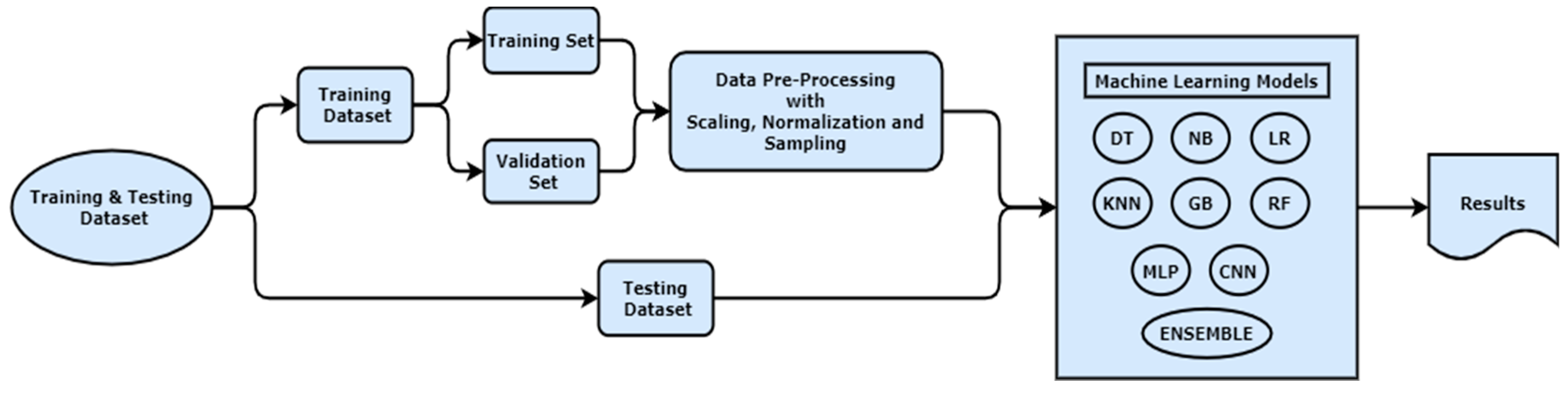
3. Materials and Methods

In terms of a general overview, the testbed environment comprises five integral components of network infrastructure, simulation of IoT devices, extraction of network data and features, tools and techniques required for a botnet attack, and machine learning approach for attack/normal network classification.

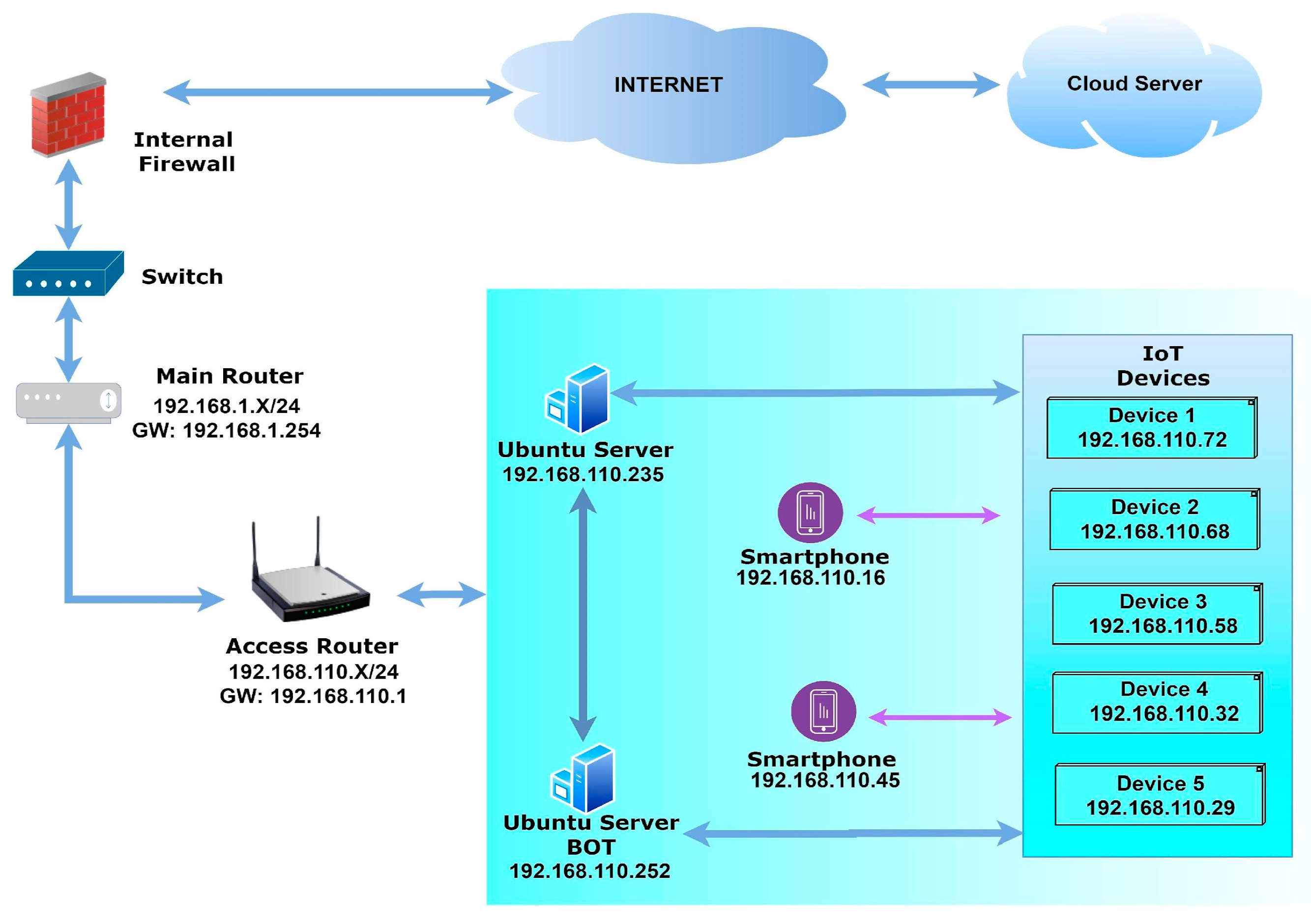
3.1. Details of the Testbed

The network infrastructure in the testbed enables the incorporation of two Linux servers that use Ubuntu version 20.04, also commonly known as Focal Fossa. This helps the inclusion of normal and attack machines with supportive devices such as routers and switches. The server, IoT devices, and smartphones are connected to WAN and LAN interfaces accordingly and are connected to the Internet through a combination of routers and a switch. Figure 1 illustrates the network architecture components of the testbed.

The system follows the Message Queuing Telemetry Transport (MQTT) [21] and HTML protocol while servicing through the gateway API and is programmed accordingly using scripts programmed in Java. A particular Ubuntu Server is under the control of the attacking entity, and its purpose is to execute various types of Botnet-related attacks, such as port scanning, fingerprinting, and volumetric and protocol-based DDoS attacks. The transmission of essential data and information between servers was facilitated by employing the File Transfer Protocol (FTP), a secure method for transferring files over a network that utilizes the Secure File Transfer Protocol (SFTP) operating on port number 22. The comprehensive dataset of both benign and malicious network traffic was meticulously captured using Wireshark [22], a proficient network packet analyzer tool that runs on the Ubuntu operating system. Wireshark captures packet information on demand, ensuring the entire volume of network traffic data is precisely captured. The cloud server utilizes the cloud server platform known as Heroku. In this cloud server, Heroku references the repository of a Java program uploaded to Gitlab (https://about.gitlab.com/ assessed on 1 May 2023). Heroku supports the programming language and can process the system following the Java-based framework, Spring boot. While processing, the Heroku server also manages the internal program data in one popular and cost-effective database platform, PostgreSql (https://www.postgresql.org/ assessed on 1 May 2023). The data generated from the IoT device follow the network communication protocol to transfer and receive files from the Heroku server [23]. The Representational State Transfer Application Programming Interface (RestAPI) integration through java programming helps the IoT device to communicate with its web and android based application to retrieve and transfer the necessary data. Figure 2, illustrating the communication process for IoT network.

The following are the primary microcontroller components utilized for the development of the IoT device: (1) Arduino Uno, (2) SIM808 Module, (3) ESP8266 (NodeMCU), (4) Load Cell Sensor, and (5) HX711 Module.

The IoT device is programmed through Arduino IDE, implementing the C++ programming language for the following functions:

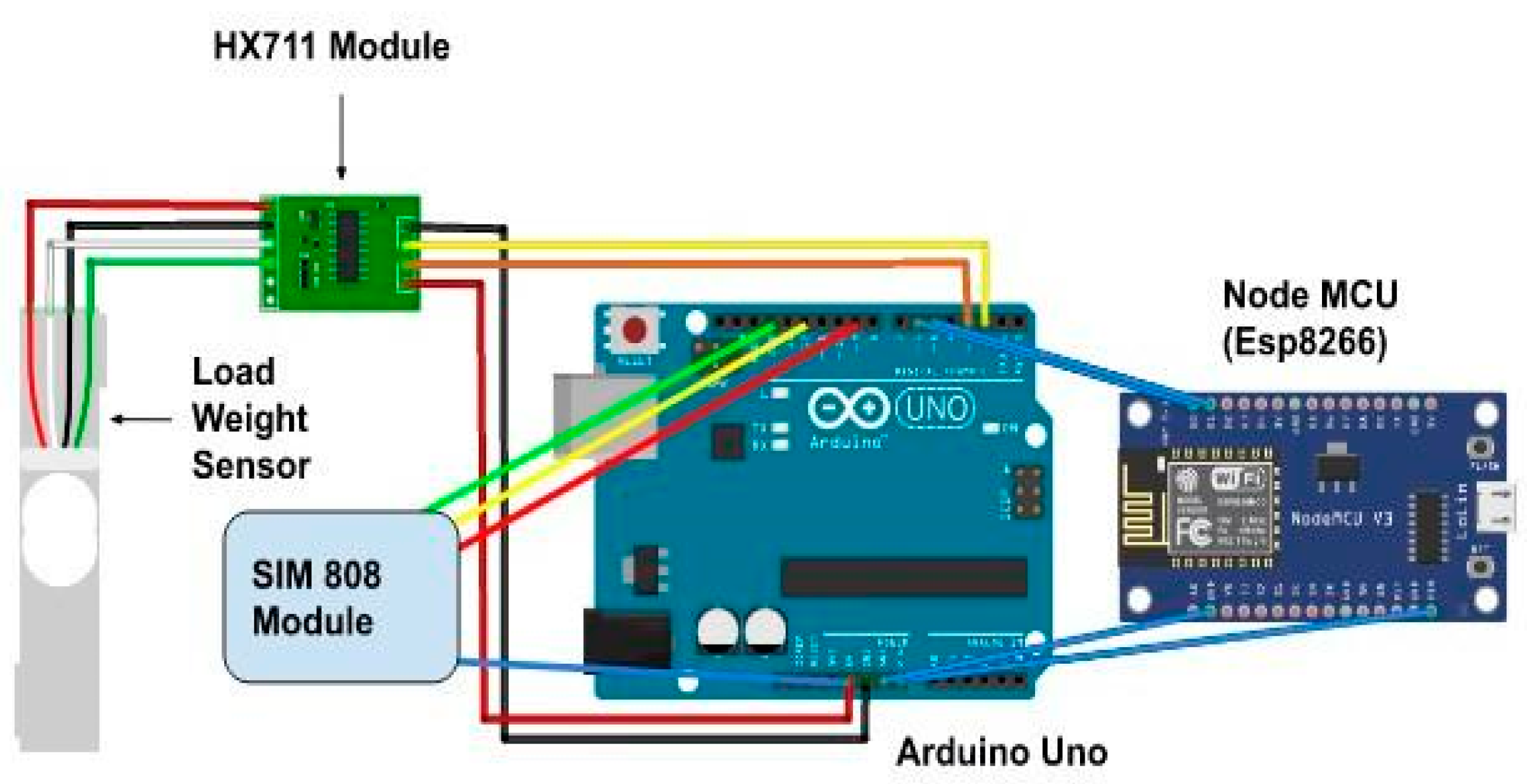
• Arduino Uno’s communication with all four components and supporting accessories;
• Sim808 Module for GPS location-based information retrieval and GSM (Global System for Mobile Communication) utilization for cellular network use;
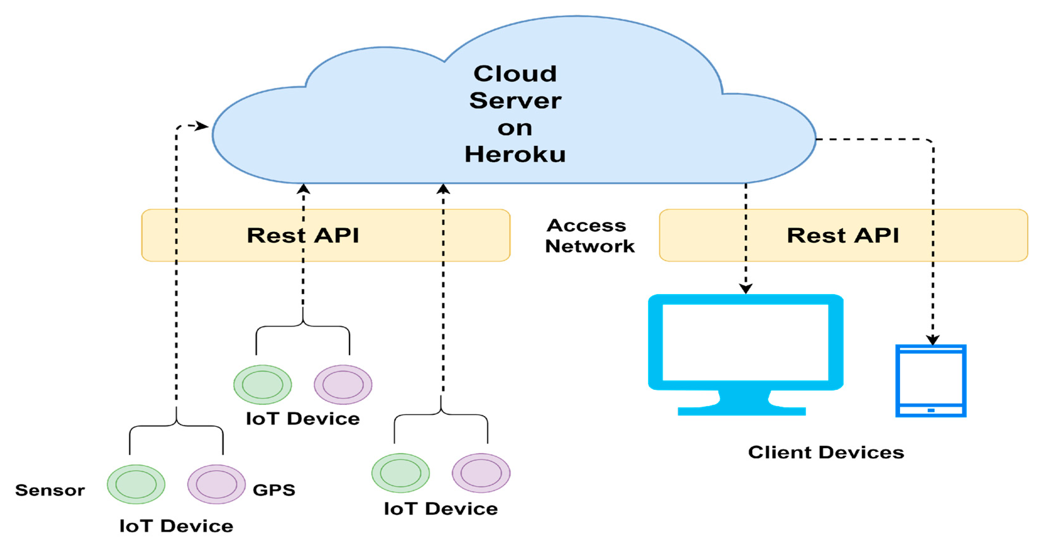
• Esp8266, which helps the WiFi network communication to initialize the communication between the IoT device with the cloud network;
• The Load Cell Sensor and HX711 Module help generate the sensor data based on an object’s weight over the sensor. The HX711 module converts the analog signal from the sensor and amplifies the voltage output from the load sensor so that Arduino Uno can read the output. Algorithm 1 outlines the procedure utilized for the communication of cloud network with developed IoT devices.

Algorithm 1 Transmitting data from SIM808 to cloud network

1: Connect the SIM808 module to the Arduino Uno using the appropriate pins and connectors

2: Configure the SIM808 module with the appropriate settings and credentials for the cloud network

3: Use the Arduino Uno’s serial communication functions to establish a connection with the SIM808 module

4: Use the SIM808 module’s API to obtain the data that you want to transmit

5: Use the Arduino Uno’s networking functions (such as WiFiClient or EthernetClient) to establish a connection with the cloud network

6: Use the Arduino Uno’s HTTP or MQTT libraries to send the data to the cloud network

7: Disconnect from the cloud network and the SIM808 module when the transmission is complete

For simulation, both the weight and GPS sensors are programmed to continuously provide the data to the cloud server, hence helping with the optimal level of data generation and storage.

3.2. Data Generation

Wireshark [22] provides normal and attack network traffic in pcap files. For data integrity, one of the tools that is used is tcpdump, which analyzes packet headers and payloads. However, this approach can be time-consuming and may become a bottleneck in high-speed networks, requiring a high processing throughput to be effective. Figure 3 depicts the block diagram of the connected devices forming an IoT device in operation.

3.2.1. Flow-Based Approach

The flow-based approach looks at high-level descriptions of communication between devices and can be more efficient, reducing the amount of information that needs to be analyzed [24]. In this research, packet-based data from the network were converted into a flow-based format using the Argus tool in order to facilitate machine learning-based approaches at a convenient scale [25].

While IoT devices generally communicate with the required server over the Internet, normal and attack traffic, in particular, need to be executed simultaneously. This requires a particular Wireshark tool to capture raw packet data and store them physically in the Ubuntu Server. As the testbed environment is experimental and it is clear which IP address belongs to the attack traffic, it is more convenient for the job to observe the data once generated.

3.2.2. Packet Conversion

While the continuous volumetric and protocol-based botnet attack is carried out in the system with tools such as the Goldeneye tool [26], assisted by Hping3 [27] and Nmap [28] for port filtering and accessing, the pcap files get captured and are stored. Moving forward, a successive flow-based formatting is required where the Argus tool is used. Conversion of packet data into the Argus file is performed by its keyword,

/argus -r networkData.pcap -w networkArgData.argus

Argus follows the command of -r to read and -w to write into the required files. After Argus provides the network flows in a file format, another command helps with the generation of the csv files. The different fields captured from the net workflow help determine the behavior of the packet, and thus, the results are categorized accordingly through the following command:

/ra -c, -s *Provide the necessary header files for csv* -r filename.argus¿filename.csv

This starts the Argus daemon, and necessary resources are provided to convert the Argus file to a csv file with the required fields. A total of six different CSV files were created with both normal and attack traffic with the required fields, as provided by the Argus Client. Figure 4 demonstrates attacks on the communication channel across different protocols.

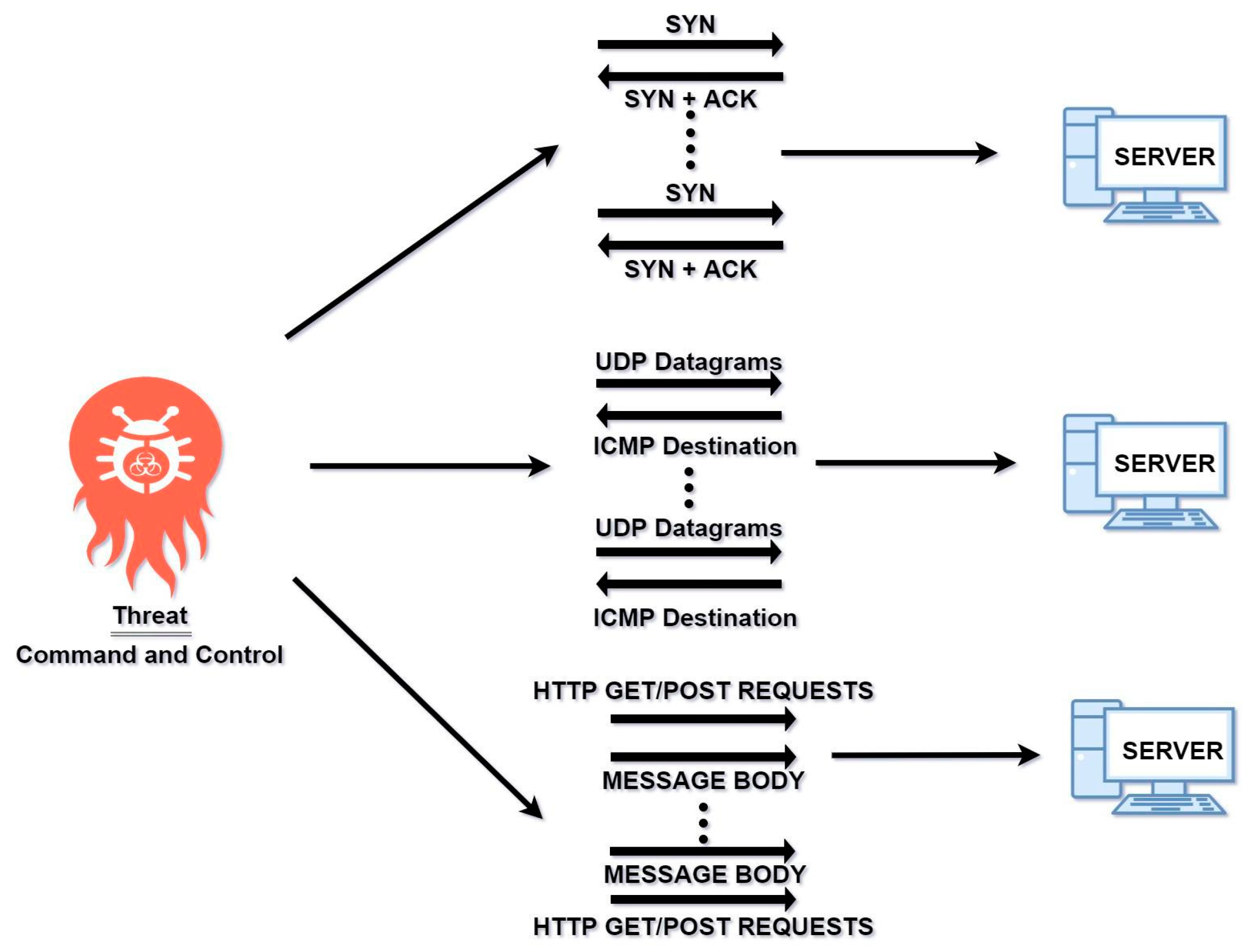
3.3. Initiation of Botnet Attack

The steps taken for the botnet attack in the testbed can be categorized into the following stages:

3.3.1. Denial of Service

In a denial of service (DoS) attack, an attacker attempts to make a network resource or service unavailable to its intended users by overwhelming it with traffic or disrupting its normal functioning. DoS attacks can take many forms, including flooding the targeted server with requests, sending malformed or malicious packets to the server, or exploiting vulnerabilities in the server software to crash the server. DDoS and DoS are inherited for the dataset using TCP, UDP, and HTTP protocols.

The Hping3 tool was utilized for the process of DDoS and DoS attacks on the TCP and UDP protocol using the following command:

hping3 -syn -flood -d 100 -p 80 192.168.110.235, where syn signifies SYN TCP attack, flood signifies the packets’ rapid flow, d is the packet size, and p provides the value of port.

The Goldeneye tool was utilized for the attack on HTTP protocol using the following command:

goldeneye.py http://192.168.11.235:80 -m post -s 75 iw 1 assessed on 25 April 2023, where m provides the information of obtaining a get request or post request, 80 is the port number, s provides the number of sockets information, and w is the simultaneously working mechanism.

3.3.2. Network Discovery/Reconnaissance Attack

A network discovery attack is a type of cyber/Internet attack in which an attacker sends probe packets to a target network or system in order to gather information about the system’s configuration, vulnerabilities, or available services. Network discovery attacks can be used to gather intelligence for more sophisticated attacks, such as DoS attacks or network intrusions [29]. Network discovery attacks can take many forms, including ping sweeps, port scans, and banner grabbing. Network discovery attacks can be challenging to detect as the probe packets may not contain malicious payloads or raise alarms in traditional security systems. Therefore, it is important for organizations to implement a comprehensive security strategy that includes monitoring for probe packets and other indicators of potential network discovery activity [29].

PortScanning: Nmap and Hping3 were utilized for this process, performing the required port scans by using the following commands:

nmap -sT 192.168.110.235, where sT connects to the TCP protocol of the IP address mentioned. Likewise, Hping3 also uses the command nmap -S -scan 1-1000 192.168.110.235, where S signifies SYN scan and provides the range of scan needed.

OS fingerprinting: Here, Nmap and XProbe2 [30] tools were utilized for different levels of OS scans. Nmap tool with Xprobe2 as a functional dependency work to identify the OS of the target as follows:

nmap -sV -T5 -PO -O 192.168.110.235, where sV signifies SYN scan, T5 suggests the scan is possible, PO includes IP protocol ping packets, and O enables the scanning. Tools utilized for the initiation of botnet attacks are tabulated in

Table 2. Tools utilized for botnet attacks.

Reconnaissance	Denial of Service
Service Scanning-nmap, hping3	DDoS-hping3, goldeneye
OS Fingerprinting-nmap, Xprobe2	DoS-hping3, goldeneye

.

3.4. Labeling of Dataset

Ostinato [31] is a network packet and traffic generator and analyzer. It is utilized in the Ubuntu server as a complementary network analyzer for Wireshark, and it can also be installed as an add-on to the application. Ostinato is utilized to create custom packet streams in conjunction with Wireshark and Argus to label datasets. By configuring Ostinato to generate specific types of network traffic, Wireshark to capture the packets, and Argus to record the packet flows, the datasets are labeled. For botnet network data, each traffic generated is recorded according to the attack performed. Ostinato helps mostly in smaller testbeds as the condition of only single entity dataset generation is handled by the dataset generator from Ostinato, which can generate and analyze the dataset accordingly at the same time. The table below provides information on the utilization of Ostinato in the area of botnet attack labeling. Each packet transaction through each type of botnet is labeled according to the timetable of the activation of the botnet attack.

Table 3. Attack and normal network category from labeling.

TrafficCategory	SubCategory
Normal	Normal
DoS	TCP, UDP, and HTTP
DDoS	TCP, UDP, and HTTP
Reconnaissance	ServiceScan and OSFingerprint

labels network traffic categories, subcategorized by the implemented botnet technique, alongside normal network traffic.

3.5. Analyzing the Dataset

As previously noted, the dataset comprises a variety of attack topologies. To understand the dataset’s complexity, an evaluation of simulated traffic hours utilizing all of the gathered characteristics in the various network levels was initiated.

Figure 5 shows the exact trace of how a file named network.pcap on a simulated environment can store packet data over time. Figure 6 provides data percentage statistics of the degree of data characteristics. The Denial of Service (DoS) comprises the highest percentage of the dataset, at 38%, whereas the Reconnaissance attack comprises the least, at 11%, in the generated dataset. The Dos and DDoS records hold the highest value due to the involvement of all three TCP, UDP, and HTTP attacks from the simulated environment. The Reconnaissance attack has the Service Scan and OS Fingerprinting attacks on its sub-categories, while the normal network is the simulated network without any intervention of botnet threats in the simulated environment.

The generated dataset comprises 44 different features, including the category and sub-category of attack network data. For each DDoS and DoS, the sub-categories of UDP, TCP, and HTTP are included, while the Reconnaissance attack carries the OSFingerprinting and ServiceScan. Analysis of the dataset is also inclined to select features of datasets to analyze optimal features and aid in machine learning for the comprehensive identification of cyberattacks. The analysis of datasets using correlation coefficient measures is an important task to measure the strength of the relationship between two or more variables in the dataset. The correlation coefficient is a statistical measure that statistically can range from −1 to 1, indicating the degree of interconnected correlation between variables.

The total dataset features, along with their respective description, is listed in Appendix A.

3.5.1. Pearson Correlation Coefficient

This is a measure of the linear correlation between two variables. It determines the strength and direction of the relationship between two variables. By dividing the covariance of two variables by the sum of their standard deviations, the Pearson correlation coefficient is determined. The scale ranges from −1 to 1, with −1 denoting a strong negative correlation, 0 denoting no association, and 1 denoting a high positive correlation [32]. The Pearson correlation coefficient is commonly used in datasets because it is easy to understand and calculate, and it can be used to identify relationships between continuous variables. It is implemented in the dataset as it provides its advantage in feature selection and dimensionality reduction. The equation for the Pearson correlation coefficient is as follows:

$$r_{XY}=\frac{\sum _{i=1}^n(X_i-\overline{X})(Y_i-\overline{Y})}{\sqrt{\sum _{i=1}^n(X_i-\overline{X}{)}^2}\sqrt{\sum _{i=1}^n(Y_i-\overline{Y}{)}^2}}$$

(1)

where $\overline{x}$ signifies the sample mean of variable x, and $\overline{y}$ signifies the sample mean of variable y. To find the correlation between the features in a dataset, a script in Python to examine the correlation coefficient was created, and the attributes were ranked in a range of −1 to 1. The average correlation for each feature was also computed to identify the features that would introduce less uncertainty in the dataset. When there is a strong relation between two features, one feature from the pair can be eliminated. Hence, if there is a strong relation, the value of the pair comes close to 1, which signifies that X is highly correlated to Y, while a value close to −1 suggests a negative correlation. If there is no correlation, then the correlation coefficient provides the result of 0 [32]. In the dataset, the threshold was set to 0.90, as it helps obtain the highly correlated feature from the set and helps in the feature reduction. One of the pairs with a threshold greater than or equal to 0.90 was eliminated, and also the correlation relation between each of the different variables opposed to the target was also considered in the research. Figure 7 shows the Pearson correlation heatmap for the dataset where every feature pair with a higher or equal to 0.90 correlation is dropped for the machine learning model training.

3.5.2. Entropy

In the context of classification in supervised learning, entropy is often used to measure a group’s impurity. It is used to analyze the relevance of a split in a decision tree, where the goal is to select the split that results in the most homogeneous subgroups (i.e., sub-groups with the lowest entropy) [33]. Overall, the use of entropy in classification helps to identify splits that result in more homogeneous and pure sub-groups, which can improve the accuracy and effectiveness of the model. The choice of the best entropy measure for a particular problem depends on the specific requirements and characteristics of the problem. In the context of classification in supervised learning, Shannon entropy is the most commonly used entropy measure. It is defined as the sum of the probabilities of all possible outcomes multiplied by the log of the probability of each outcome. It provides a simple and intuitive way to quantify the impurity of a group, and is effective in decision tree learning and other classification algorithms [33]. The equation for Shannon entropy is as follows:

$$H\left(X\right)=-\sum _{i=1}^n{p}_{xi}{\log }_2{p}_{xi}$$

(2)

where H(X) represents the Shannon entropy of the random variable X, n is the number of possible outcomes of X, and p(xi) is the probability of the i-th outcome of X. The features obtained are characterized according to the entropy value, where a lower entropy provides the idea of higher information gain. This way, with a Python script, the best features are selected according to the entropy calculated. The best 10 and 20 features from both datasets are shown below in

Table 4. Best 10 and best 20 features of the generated dataset.

Best 10 Features	Remaining 10 Features for Best 20
RecMean	FlowSrcIPRate
RecMin	FlowDstIPRate
RecMax	SrcPortRate
FwdPackets/s	DstPortRate
BwdPackets/s	SrcIpPktsCount
SrcIPFwdConn	DstIpPktsCount
DstIPBwdConn	BwdPktsCount
FlowID	ProtocolNum
FlowState	RecordTime
ArgusSeq	FwdPktsCount

.

This research employs the idea of multiclass classification through cross-evaluation of the proposed dataset with one of the most popular botnet datasets, BoT-IoT [17]. Feature reduction for the BoT-IoT dataset is also crucial for a comprehensive machine learning analysis. The researchers and the team at the University of New South Wales (UNSW) provided detailed information about the dataset and utilized techniques such as correlation coefficient and chi-square tests to identify the best features for their dataset. These methods allowed for the reduction of the dataset to only the most informative and relevant features, facilitating more efficient and accurate analysis. The dataset and feature information, as well as the best features, are accessible through the dataset database, which can be accessed through a web portal provided accordingly by the researchers [17]. The BoT-IoT dataset comprises a total of 46 distinct features. The best 10 and 20 features from the BoT-IoT dataset are presented in

Table 5. Best 10 and 20 features of BoT-IoT dataset [17].

Best 10 Features	Remaining 10 Features for Best 20
seq	AR_P_Proto_P_Dport
stddev	AR_P_Proto_P_DstIP
N_IN_Conn_P_SrcIP	AR_P_Proto_P_Sport
min	AR_P_Proto_P_SrcIP
state number	TnP_PSrcIP
mean	TnP_Per_Dport
N_IN_Conn_P_DstIP	TnP_PDstIP
drate	flgs_number
srate	Pkts_P_State_P_Protocol_P_SrcIP
max	Pkts_P_State_P_Protocol_P_DestIP

accordingly.

The cross-evaluation of data in this study was conducted using a BoT-IoT dataset consisting of 3 gigabytes of data. The 3 GB of the dataset contained 12% normal network traffic and 88% attack traffic. In order to optimize the analysis, the top 10 and top 20 features were utilized in the process. Figure 8 showcases the dataset statistics for 3 GB of dataset from BoT-IoT that has been implemented in the cross evaluation process.

The most frequently occurring attacks in the dataset were DDoS and DoS botnet attacks, which constituted 64% of the attacks, followed by reconnaissance attacks at 24%. This information proved to be helpful in identifying the patterns and similarities present in the generated dataset. The generated dataset contained approximately 5.2 million flows, and the utilization of the DDoS and DoS botnet attacks and reconnaissance attacks enabled a thorough analysis of the similar context of the data.

3.5.3. Data Scaling and Normalization

Scaling and normalization boost data preprocessing, which helps transform the dataset’s features into a standard scale without distorting differences in the range or magnitude of the features. Standard Scaler, a data preprocessing module from the scikit-learn library, was utilized in this study to provide transparency in the mean and unit variance between the features. This also enables the improvement of the algorithm’s performance by ensuring that the input features are on a similar scale and possibly have Gaussian distribution. Scaling also helps reduce the computational burden of training the algorithm, and normalization can make it easier to compare features measured on different scales. It is a technique for scaling the features of a dataset so they have zero mean and unit variance [34]. The formula for z-score normalization is as follows:

$$z_i=\frac{xi-\mu }{\sigma }$$

(3)

where x represents the original data point, µ (mu) is the mean of the sample of the data points, σ (sigma) is the standard deviation, and z is the standardized data point. This formula subtracts the mean of the feature from each value and divides the resulting values by the standard deviation of the feature. This helps to enable the components to be normalized at the same level of scale, transform features with skewed distributions, reduce the influence of outliers on the features, and make a larger dynamic range of distance measurement stable, which reduces the computational burden while training the model.

3.5.4. Sampling of Data

As the system’s goal is to identify unusual events, it is common for these types of datasets to be imbalanced, with a higher chance of a minority of instances being classified as normal networks and the majority being classified as attack activity. Imbalanced datasets can be challenging to work with because the classifier may not have enough examples of the minority class to learn how to classify them accurately. This can lead to poor performance in the minority class and make it difficult to evaluate the classifier’s performance using standard metrics, such as accuracy. Several approaches address imbalanced datasets, including oversampling the minority class, undersampling the majority class, and using specialized algorithms designed to handle imbalanced datasets. Considering a variety of samples, the imbalanced dataset was split into a number of classes with different samples using the idea of oversampling. Random Over Sampler is an oversampling technique the imblearn library provides for balancing imbalanced datasets [35]. It works by generating synthetic samples of the minority class by randomly sampling from the existing minority class samples. This helps create different classes of various samples in the training set. A total of nine different classes were taken for the multiclass problem, where each class belongs to the nature of the attack or normal network from the dataset.

Table 6. Class categorization for multiclass classification.

Classes	Nature
0	DDoS-HTTP
1	DDoS-TCP
2	DDoS-UDP
3	DoS-HTTP
4	DoS-TCP
5	DoS-UDP
6	Normal
7	ServiceScan
8	OSFingerprint

shows the different categorizations of class for multiclass classification that were used for the research.

4. Results

This chapter describes the various techniques utilized to obtain results for binary and multiclass classification for the generated dataset and cross-evaluate the dataset with BoT-IoT [17]. This study suggests the idea of cross-evaluating the generated dataset with one of the most popular datasets, where the results discuss the performance measuring metrics, such as confusion matrix, precision, recall, F1-score, accuracy, ROC, and AUC curve, as well as model parameters, for different machine learning models. The chapter also includes a comparison of binary classification for IoT datasets using the best 10 and 20 features, and a comparison of the performance of different machine learning models in binary classification using a confusion matrix for the best 20 features. It also covers the optimal feature selection for cross-dataset multiclass classification using the best 10 and 20 features. These techniques are used to obtain and analyze the results to conclude the performance of the models.

4.1. Performance Measuring Metrics

A range of performance indicators was commonly utilized to assess the effectiveness of different machine learning models. These indicators provided insight into a model’s capabilities and limitations, and were used to compare the performance of different models. By examining these metrics and concepts, a thorough understanding of a model’s performance helped to gain the insights needed for an informed decision about which model was most suitable for a given task. The metrics are formulated as follows:

$$Precision \left(P\right)=\frac{\mathrm{T}\mathrm{P}}{\mathrm{T}\mathrm{P}+\mathrm{F}\mathrm{P}}$$

(4)

$$Recall \left(R\right)=\frac{\mathrm{T}\mathrm{P}}{\mathrm{T}\mathrm{P}+\mathrm{F}\mathrm{N}}$$

(5)

$$Accuracy \left(A\right)=\frac{\mathrm{T}\mathrm{P}+\mathrm{T}\mathrm{N}}{\mathrm{T}\mathrm{P}+\mathrm{F}\mathrm{N}+\mathrm{T}\mathrm{N}+\mathrm{F}\mathrm{P}}$$

(6)

$$F1 Score \left(F1\right)=\frac{2·PR}{P+R}$$

(7)

where True Positive (TP) is the number of actual attack records that were correctly identified as attacks, True Negative (TN) is the number of actual normal records that were correctly identified as normal, False Negative (FN) is the number of actual attack instances that were not correctly categorized as normal, and False Positive (FP) is the number of actual normal instances that were incorrectly identified as attacks. Furthermore, the training time (i.e., the CPU time to create the model) and prediction time (i.e., the CPU time to test the model) are also examined since they are crucial in evaluating the model’s execution time, particularly in the durational phase of runtime and testing time to report the projected outcomes.

4.2. Model Parameters

The data were effectively processed, and then machine learning algorithms were employed to assess how well they performed on the dataset. These models included decision trees, logistic regression, naive bayes, random forests, k-nearest neighbors, gradient boost, a multi-layer perceptron, and a convolutional neural network. The Python scripts were implemented using the scikit-learn library, and the model parameters were adjusted to achieve the highest accuracy while minimizing training time. The specific model parameters used for each classification model are provided in subsequent sections. Figure 9 demonstrates the processes utilized for the dataset evaluation through machine learning models.

4.2.1. Decision Tree

The model classifier was created using the scikit-learn DecisionTreeClassifier. The model’s maximum depth was set to 2, while all the other parameters were left at their default settings. The test sample was taken to represent 20% of the entire dataset after the data were standardized using the StandardScaler function in the scikit-learn library.

4.2.2. Naive Bayes

Scikit-learn classifier GaussianNB was utilized as the model classifier for the Naive Bayes. All the supporting features were utilized with default values. The data were scaled by StandardScaler and normalized with Z-score normalization from the scikit-learn library, where the test sample was considered to be 20% of the total data.

4.2.3. Logistic Regression

The classifier LogisticRegression was implemented from the linear model library of scikit-learn. In the case of the LogisticRegression function in Python’s scikit learn library, the solver parameter specifies the algorithm to use when fitting the model. The solver was specified with liblinear such that the model would use the LIBLINEAR library to fit the model. LIBLINEAR is a linear classifier that can handle both binary and multiclass classification problems, well suited for cases where the number of features is very large relative to the number of samples. The test sample was taken into account as 20% of the entire dataset after the data were normalized using StandardScaler in the scikit-learn library.

4.2.4. KNN

The KNeighborsClassifier algorithm from the scikit-learn library was utilized under the library of neighbors. The total number of neighbors was set as 30 to attain the best balance between model performance and computational efficiency. The distance metric was determined with default values for the Euclidean distance. The algorithm was set to ‘auto’ such that the most reasonable algorithm based on the circumstances of statistics passed would be supplied in the fitting of the model. Number of test samples was set to 0.20, with Z-Score normalization utilized for the data preprocessing.

4.2.5. Gradient Boost

The XGBClassifier was utilized as the model training classifier from the library of xgboost, and an instance of the class was created with 42 random states. The random state parameter specifies the random seed used to initialize the model. The data were scaled by StandardScaler and normalized with Z-score normalization in the scikit-learn library, and the test sample was considered to be 20% of the total data.

4.2.6. Random Forest

The RandomForestClassifier was utilized from the scikit-learn library to implement the model. The n_estimators were specified to be 10, providing the number of trees in order to obtain the most comprehensive accuracy levels as 10 with entropy as the criterion passed to the model. In a random forest, entropy is used as a criterion for splitting the data at a node. When the entropy of a node is high, it means that the data at that node are not pure and contain a mix of different classes. This indicates that the node can be split further to create more homogeneous sub-nodes. For multiclass classification, the n_estimator utilized is 100. The data were normalized with StandardScaler, and the test sample was collected to be 20% of the total data.

4.2.7. MLP

The MLPClassifier in the neural network class of the scikit-learn library was utilized to train the model. A single hidden layer was specified with 100 neurons, with the alpha being 0.0001, to observe the highest possible accuracy in the data analyzed. The alpha value can help prevent the weights from becoming too large, which can lead to numerical instability during training. For multiclass classification, three hidden layers, with 100 as the first neuron, 100 as the second neuron, and 50 as the third neuron, were utilized for the classification. Additionally, the alpha value for multiclass classification was specified as 0.0001.

4.2.8. CNN

The Tensorflow module was implemented for defining and training the model. The keras module provides a high-level API for building and training neural networks, which is implemented to provide the Sequential class. The MinMaxScaler class was implemented to normalize the input data before feeding it to a neural network model. The test sample was collected to be 20% of the total size. The model consisted of a sequence of seven dense layers followed by six dropout layers. Each dense layer was fully connected and had a specified number of nodes, as well as a specified activation function. The range of dense layers started with 1500 nodes, and the dropout layers were a type of regularization layer that helped to prevent overfitting by randomly setting a fraction of the input units to zero during training. The last layer of the model was a dense layer with a single node and a sigmoid activation function, which was used for binary classification. The model was compiled using the compile method, which specified the loss function, optimization algorithm, and metrics to track during training and evaluation. The research implemented the categorical_crossentropy loss function with epochs of 50 under a very popular adam optimizer. The dense layers were optimized by the regularization technique and fine-tuning. The dropout layers prevent overfitting by adding constraints to the model.

4.2.9. Ensemble Method

The VotingClassifier from the scikit-learn library was implemented to train an ensemble model that utilizes the predictions of multiple classifiers using both hard and soft voting schemes. The VotingClassifier is initialized with a list of estimators (i.e., the individual classifiers) and a voting type. The fit method is used to train the ensemble model on the training data. The score method is used to evaluate the performance of the ensemble model on the test data. The ensemble model is trained using seven different classifiers: model 1 (a decision tree), model 2 (a Naive Bayes classifier), model 3 (a logistic regression classifier), model 4 (a KNN classifier), model 5 (a random forest classifier), model 6 (a gradient boosting classifier), and model mlp (a multi-layer perceptron classifier). The hard voting scheme means that the ensemble model will make a prediction based on the majority vote among the individual classifiers, while the soft voting analyzes the average of class probabilities. Algorithm 2 explains the hybrid voting ensemble technique, which implements both the hard and soft voting techniques from the classifiers involved in the ensemble process.

Algorithm 2 Hybrid Voting Ensemble using Hard and Soft Voting

Require: Training data D = (x1, y1), (x2, y2),…, (xn, yn), test data T = x’1, x’2,…, x’m

Ensure: Ensemble predictions ŷ = ŷ1, ŷ2,…, ŷm

1: Train K models on the training data D: M = M1, M2,…, MK

2: for each test instance x’i do

3: for each model Mj ∈ M do

4:  Make a prediction ŷi,j = Mj(x’i)

5: end for

6: Compute the average of class probabilities avg(y) = (1/K) Σj = 1K pi,j(y), where      pi,j(y) is the probability estimate for class y given by model Mj for instance x’i

7: Compute the majority vote prediction ŷivote = argmaxy Σj = 1K [ŷi,j = y]

8: Compute the average prediction confidence Ciavg = (1/K) * Σj = 1K maxy pi,j(y)

9: Set a threshold α ∈ [0, 1]

10:  if the average prediction confidence Ciavg ≥ α then

11:   Set the ensemble prediction to be the average prediction:       ŷi = arg maxy pˆiavg(y)

12: else

13:  Set the ensemble prediction to be the majority vote prediction: ŷi = ŷvotei

14:  end if

15: end for

16: return ŷ = 0

In this research, while the employment of a machine learning model for binary classification relies solely on the generated dataset, utilizing its top 10 and 20 features, the concept of multiclass classification involves merging the two datasets of the generated dataset with the BoT-IoT dataset, each with a size of 3 gigabytes, for the purpose of conducting the analysis. Cross-evaluation of datasets was utilized with similar sizes of data to avoid biased results and ensure that the model generalizes well to new data. It is important to comprehend that using datasets of equal size can help prevent overfitting to a particular dataset or set of features. The binary and multiclass classification approaches are implemented with distinct sets of parameters, which are enumerated in

Table 7. Parameters employed for binary and multiclass classification.

Classifiers	Binary Parameter	Multiclass Parameter	Approach	Scikit Classifier
Random Forest	n_estimators = 10 criterion = ‘entropy’	n_estimators = 100 criterion = ‘entropy’	Multiclass = ‘OVR’	RandomForestClassifier
KNN	n_neighbors = 30	n_neighbors = 30	Multiclass = ‘OVR’	KNeighborsClassifier
MLP	1 hidden layer and 100 neurons, alpha = 0.0001	3 hidden layers (100, 100, 50), alpha = 0.0001	Multiclass = ‘OVR’	MLPClassifier
Decision Tree	Only Multiclass Classification	max_depth = 2, criterion = ‘gini’	OVR	DecisionTreeClassifier
Gradient Boost	Only Multiclass Classification	random_state = 42	One-vs-Rest approach (OVR)	XGBClassifier
Naive Bayes	Only Multiclass Classification	var_smoothing = 1 × 10−9	OVR	GaussianNB
Logistic Regression	Only Multiclass Classification	solver = ‘liblinear’	OVR	LogisticRegression
CNN	Only Multiclass Classification	7 dense layers, 6 dropout layers, 1500 nodes, epochs: 50, activation function: ‘relu’, loss_function: ‘categorical_crossentropy’ optimizer: ‘adam’	Categorical	Tensorflow-Sequential Model
Ensemble	Only Multiclass Classification	voting = ‘soft’ and ‘hard’, estimators = ‘7’, sklearn.ensemble technique	OVR	VotingClassifier

.

4.3. Binary Classification for Generated Dataset

The primary dataset from the designed IoT device was utilized for this process of binary classification, where further multiclass classification will be analyzed with the help of the BoT-IoT dataset in the next sections. Using the above-mentioned machine learning approaches, binary classification was carried out to determine if a data sample was hostile or not. Using the assessment metrics specified in the following section, the results are tabulated for various numbers of features. The 10 and 20 best features were selected to be evaluated. The top features to help with categorization were those that substantially influenced the decision-making process.

4.3.1. Best 10 Features

Shannon entropy was used to identify features that contained a high level of information about the target variable, while the Pearson coefficient for correlation was used to identify features that were highly interrelated with the target variable. Combining these methods, the best 10 or 20 features were selected for training the machine learning model. The machine learning algorithm was trained on the best features to predict the presence of an intrusion. Using the best 10 or best 20 features helped achieve optimal outcomes for intrusion detection on the dataset. This was because the machine learning algorithm could avoid overfitting to noisy or irrelevant data and focus on the most informative features for intrusion detection.

The specific techniques and parameters used may vary depending on the dataset’s characteristics and the specific application of the machine learning model. Overall, the combination of Shannon entropy and the Pearson coefficient for feature selection and training machine learning algorithms on the best 10 or best 20 features led to accurate predictions of the presence of an intrusion in the dataset.

Table 8. Comparison of binary classification of best 10 features.

Model	0/1	Precision	Recall	F1-Score	Accuracy	Training Time (s)	Prediction Time (s)
Random Forest	0 1	0.5525 0.9999	0.9983 0.9681	0.7135 0.9834	0.974125	825.36	729.16
KNN	0 1	0.9992 0.9998	0.9954 1.0000	0.9973 0.9998	0.999812	996.15	562.12
MLP	0 1	0.9989 0.9998	0.9965 0.9999	0.9976 0.9999	0.999816	1256.21	24.25

presents a comparison of ML models for classification, using best 10 features from generated dataset.

4.3.2. Best 20 Features

These features were selected based on their correlation with attack instances in the dataset. By using these 20 features, machine learning models were trained to identify patterns and detect intrusions with high accuracy. The use of these features provided a more efficient and effective way to detect intrusions compared to using all the available features, as tabulated in the following table. This is because the selected features are highly correlated with attack instances and provide a more focused approach to intrusion detection. Table 5 offers a concise overview of the best 10 and 20 features. In contrast,

Table 9. Comparison of binary classification of best 20 features.

Model	0/1	Precision	Recall	F1-Score	Accuracy	Training Time (s)	Prediction Time (s)
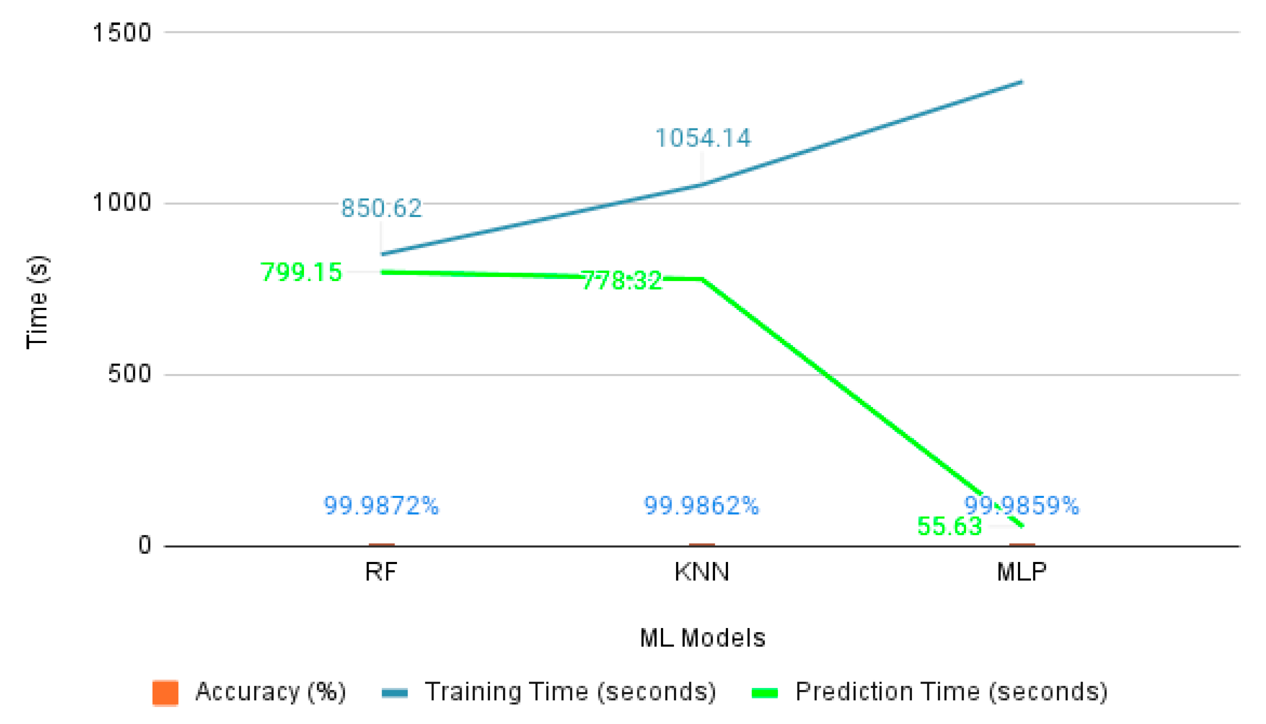
Random Forest	0 1	0.9989 0.9999	0.9976 1.0000	0.9983 0.9999	0.999872	850.62	799.15
KNN	0 1	0.9999 0.9999	0.9966 1.0000	0.9982 0.9999	0.999862	1054.14	778.32
MLP	0 1	0.9998 0.9999	0.9988 1.0000	0.9992 0.9999	0.999859	1356.14	55.63

presents a comparative analysis of machine learning models for classification, utilizing the best 20 features from the generated dataset.

4.3.3. Performance Evaluation Regarding Number of Features

With the increase in the feature set from 10 to 20, a progressive increase in overall accuracy can be observed. With random forest, we can see an exceptional increase in precision with the increase in the feature set. Additionally, the training and prediction time grows when the feature sets are increased to another 10. In KNN and MLP, both classifiers show an increase in the rate of precision and recall, which helped increase the F1-score compared to the decreased feature sets. This comparison shows a higher level of accuracy in both the feature set, where an increase in all the performance metrics can be observed, respectively, with the increasing feature set. The best 20 features observed through the information gain and entropy were utilized, where features were also dropped due to the Pearson coefficient relation. Hence, with the proper increase and a higher level of accuracy in the 20 best features, along with a slight satisfactory increase in time and prediction time measures, the optimal number of features was analyzed to be 20.

4.4. Cross-Dataset MultiClass Classification

This utilizes the cross-dataset selection of both BoT-IoT and the primary dataset that was generated. As explained previously, the BoT-IoT dataset is a very popular and well-managed dataset in the research field of the IoT. A total of 3 Gb of data from each of the datasets were merged together for this process of cross-dataset evaluation. The dataset was tested for similarity to each other, and collectively, both of the dataset features were reduced with the help of data preprocessing techniques, as discussed earlier. Figure 8 provides information about how the machine learning technique is initiated for the process. As mentioned in the classifier section, the training and testing dataset is considered 80 and 20 percent of the total merged datasets. Considering the imbalanced dataset after merging both datasets, the scaling technique was utilized to attain the highest accuracy and computational efficiency. This enables the inclusion of multiclass classification, where the samples are determined according to the attack class they belong to. The ML models were developed using the top 10 and 20 features to determine the most comprehensive list of features for achieving the peak level of accuracy in the ideal supporting time.

Table 10. Comparison of multiclass classification of best 10 features.

Model	Class	Precision	Recall	F1 Score	Accuracy	Training Time (s)	Prediction Time (s)
Decision Tree	0 1 2 3 4 5 6 7 8	0.00 0.39 0.58 0.00 0.00 0.51 0.00 0.00 0.57	0.00 1.00 0.57 0.00 0.00 0.89 0.00 0.00 0.27	0.00 0.56 0.58 0.00 0.00 0.65 0.00 0.00 0.37	0.428093	307.40	102.76
Naive Bayes	0 1 2 3 4 5 6 7 8	0.09 0.66 1.00 0.00 0.99 0.55 0.73 0.51 0.57	0.96 0.52 1.00 0.00 0.67 0.91 0.12 0.89 0.27	0.17 0.58 1.00 0.00 0.80 0.68 0.20 0.65 0.37	0.553320	212.16	55.24
Logistic Regression	0 1 2 3 4 5 6 7 8	0.31 0.20 0.95 1.00 0.99 0.69 0.38 0.55 0.38	0.89 0.06 1.00 1.00 0.67 0.91 0.13 0.91 0.13	0.46 0.09 0.97 1.00 0.80 0.78 0.20 0.68 0.20	0.846680	567.21	268.12
KNN	0 1 2 3 4 5 6 7 8	0.99 0.97 1.00 1.00 0.96 0.91 0.80 0.97 0.99	0.98 0.83 1.00 1.00 0.99 0.90 0.81 0.83 0.98	0.99 0.89 1.00 1.00 0.98 0.91 0.80 0.89 0.99	0.972670	2182.4	1136.56
Gradient Boost	0 1 2 3 4 5 6 7 8	0.58 0.91 1.00 0.72 0.86 1.00 0.62 0.76 1.00	0.57 0.91 1.00 0.45 0.96 1.00 0.64 0.73 1.00	0.58 0.92 1.00 0.56 0.91 1.00 0.63 0.75 1.00	0.873166	1657.5	4400.12
Random Forest	0 1 2 3 4 5 6 7 8	1.00 1.00 1.00 1.00 1.00 1.00 1.00 0.95 0.99	1.00 0.99 1.00 1.00 1.00 1.00 1.00 0.99 0.97	1.00 1.00 1.00 1.00 1.00 1.00 1.00 0.97 0.98	0.994109	2167.15	1354.12
MLP	0 1 2 3 4 5 6 7 8	0.98 0.99 1.00 0.99 0.99 1.00 1.00 0.98 0.91	1.00 0.99 1.00 1.00 1.00 1.00 1.00 0.94 0.96	0.99 0.99 1.00 1.00 1.00 1.00 1.00 0.96 0.94	0.982880	2856.12	1274.12
CNN	0 1 2 3 4 5 6 7 8	1.00 0.97 1.00 1.00 0.96 0.89 0.90 0.99 0.99	0.98 0.83 1.00 1.00 1.00 0.96 0.72 0.67 0.99	0.99 0.99 1.00 1.00 0.99 0.98 0.97 0.99 0.99	0.975160	5815.22	3514.5
Ensemble Approach	0 1 2 3 4 5 6 7 8	1.00 1.00 0.99 1.00 1.00 0.99 1.00 1.00 1.00	1.00 1.00 0.99 1.00 1.00 0.99 1.00 1.00 1.00	1.00 1.00 0.99 1.00 1.00 0.911 1.00 1.00 1.00	0.99967	9232.4	3201.12

provides the comparison of different classifiers utilized for best 10 features from the dataset.

The main motivation for incorporating the best 10 and 20 features from the dataset is the model’s improvement in performance due to less influence of noise and irrelevant information and faster training time. Reduced overfitting and more robust system architecture can also be taken as an inspiration for the process.

Table 11. Comparison of multiclass classification of best 20 features.

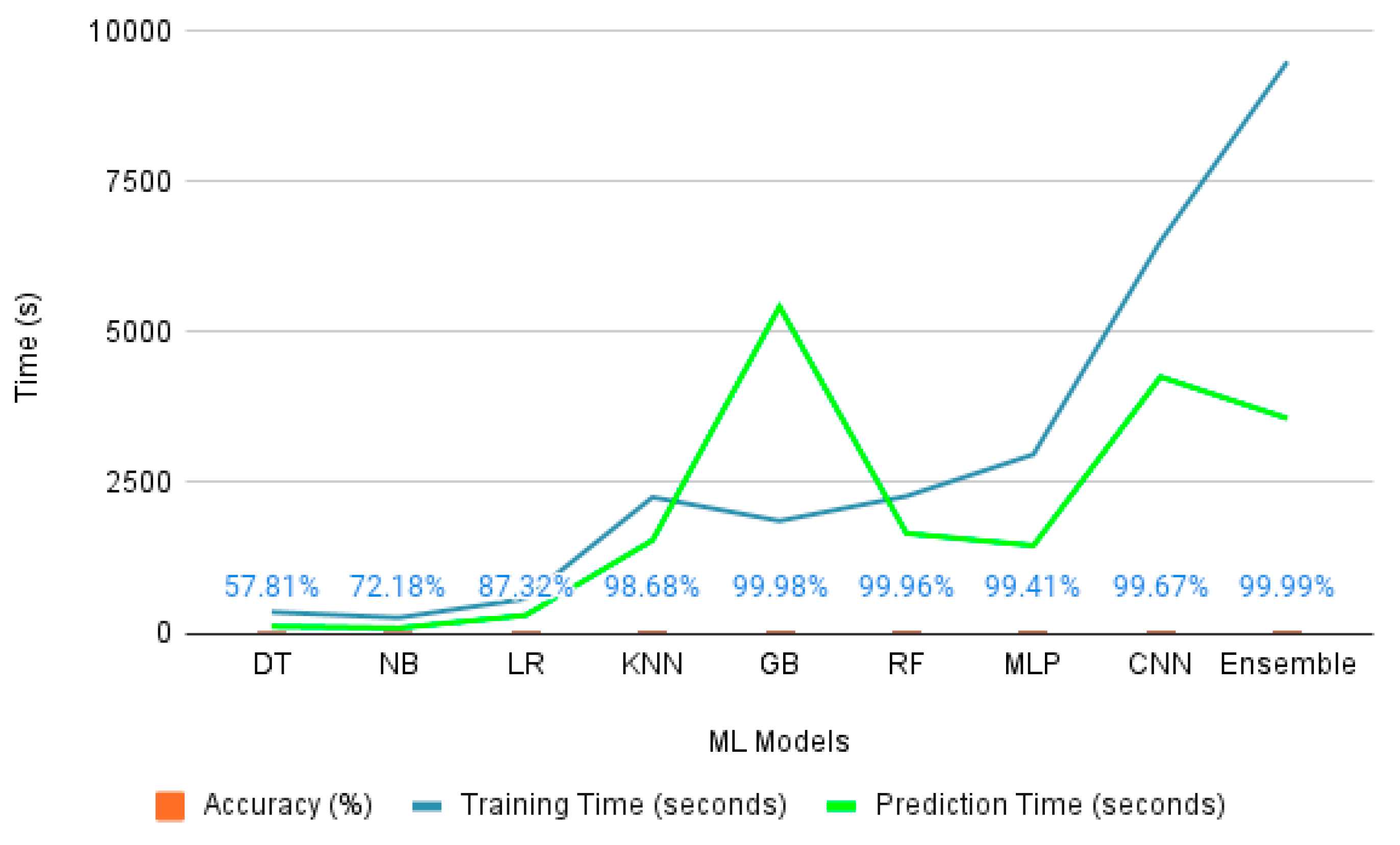
Model	Class	Precision	Recall	F1 Score	Accuracy	Training Time (s)	Prediction Time (s)
Decision Tree	0 1 2 3 4 5 6 7 8	0.00 0.39 0.90 0.00 0.00 0.70 0.00 0.00 0.57	0.00 1.00 0.87 0.00 0.00 0.92 0.00 0.00 0.68	0.00 0.56 0.89 0.00 0.00 0.80 0.00 0.00 0.62	0.578093	350.40	112.76
Naive Bayes	0 1 2 3 4 5 6 7 8	0.34 0.85 0.87 0.73 0.51 1.00 1.00 0.57 0.94	0.96 0.54 1.00 0.52 0.89 0.85 1.00 0.27 0.47	0.50 0.66 0.93 0.61 0.65 0.92 1.00 0.37 0.63	0.721787	257.32	85.67
Logistic Regression	0 1 2 3 4 5 6 7 8	0.58 0.91 1.00 0.72 0.86 1.00 1.00 0.62 0.76	0.57 0.91 1.00 0.45 0.96 1.00 1.00 0.64 0.73	0.58 0.92 1.00 0.56 0.91 1.00 1.00 0.63 0.75	0.873166	569.23	296.55
KNN	0 1 2 3 4 5 6 7 8	0.98 0.99 1.00 0.99 0.99 1.00 1.00 0.91 0.98	1.00 0.99 1.00 1.00 1.00 1.00 1.00 0.96 0.94	0.99 0.99 1.00 1.00 1.00 1.00 1.00 0.94 0.96	0.986780	2256.54	1542.26
Gradient Boost	0 1 2 3 4 5 6 7 8	1.00 1.00 1.00 1.00 1.00 1.00 1.00 1.00 1.00	1.00 1.00 1.00 1.00 1.00 1.00 1.00 1.00 1.00	1.00 1.00 1.00 1.00 1.00 1.00 1.00 1.00 1.00	0.999840	1864.25	5421.87
Random Forest	0 1 2 3 4 5 6 7 8	1.00 1.00 1.00 1.00 1.00 1.00 1.00 1.00 1.00	1.00 1.00 1.00 1.00 1.00 1.00 1.00 1.00 1.00	1.00 1.00 1.00 1.00 1.00 1.00 1.00 1.00 1.00	0.999594	2274.39	1656.34
MLP	0 1 2 3 4 5 6 7 8	1.00 1.00 1.00 1.00 1.00 1.00 1.00 0.95 0.99	1.00 0.99 1.00 1.00 1.00 1.00 1.00 0.99 0.97	1.00 1.00 1.00 1.00 1.00 1.00 1.00 0.97 0.98	0.994109	2967.15	1454.12
CNN	0 1 2 3 4 5 6 7 8	0.99 0.99 1.00 1.00 0.99 0.98 0.98 0.99 0.99	0.99 0.99 1.00 1.00 1.00 0.99 0.96 0.99 0.99	0.99 0.99 1.00 1.00 0.99 0.98 0.97 0.99 0.99	0.996718	6504.15	4254.12
Ensemble Approach	0 1 2 3 4 5 6 7 8	1.00 1.00 1.00 1.00 1.00 1.00 1.00 1.00 1.00	1.00 1.00 1.00 1.00 1.00 1.00 1.00 1.00 1.00	1.00 1.00 1.00 1.00 1.00 1.00 1.00 1.00 1.00	0.999936	9487.25	3565.21

provides the classification result utilizing best 20 features from the dataset.

In this scenario, the increase in the best features resulted in increased accuracy scores, as expected. Given the relationship between training and prediction times and the number of features, adding more features also resulted in longer training and prediction periods. The decision tree algorithm demonstrated an increase in both accuracy and training and prediction times when the features were added from 10 to 20. The decision tree algorithm performed well, with 20 best features across all classes regarding precision, recall, and F1-score. The results were similar for the random forest classifier, which also showed an increase in evaluation metrics when the features were added from 10 to 20. The prediction times for the KNN classifier were typically higher, while the training times were short and constant. The gradient boost classifier and the ensemble approach using the best 20 features also provided significant results. Overall, the findings show that, in terms of scores, training times, and prediction times, utilizing 20 features is the best choice.

5. Discussion

Regarding the binary classification of network data, the best 20 features showed an increase in classification accuracy. Only the dataset generated was utilized in the process of binary classification, where we can see that the ML models are able to identify the normal behaving network and attack network with optimal accuracy. The MLP model here takes the highest training time, but predicts quickly. In KNN, an optimal number of neighbors, as discussed in the earlier section, also enabled the model to perform accurately. Data-preprocessing techniques and Z-score normalization also play a significant role. With the imbalanced dataset, imblearn also aided the model with the best data-preprocessing analysis. On the contrary, with 99.9872%, the random forest outshines the other models and has a better average in time management as well. The classification result analysis for the generated dataset is illustrated in Figure 10.

One-vs-rest (OvR) schemes were utilized to train classifiers in multiclass classification. This involves training multiple binary classifiers to help differentiate a single class. Categorical cross-entropy loss function was utilized for the multiclass neural network classification with soft max activation for the output layer and adam optimizer for the gradient-based optimization algorithm to train multiclass convolutional neural networks. The ensemble approach was utilized as a hybrid of both the hard and soft voting techniques. Hard voting provides the majority voting for the classifier with the highest outcome, and soft voting utilizes the idea of taking the average of predicted probabilities for each class from all the ensembled classifiers. The ensemble algorithm trains different models on training data, then computes the average prediction confidence for each test instance and sets a threshold to determine which should be enacted for the outcome. Figure 11 illustrates the multiclass classification results for the cross evaluated datasets.

Table 10 and Table 11 show the multiclass classification results. The best 20 features provide the optimal results where gradient boost gives an exceptional result, and random forest also provides the optimal results with negligible errors in classifications. MLP (99.41%) and CNN (99.67%) classify the multiclass problem well. Gradient boost with 99.98% accuracy takes double or triple the prediction time when compared to the other classifiers, while random forest provides a good average in every aspect, from accuracy to time utilized. As an ensemble approach, the ensemble technique provides the optimal result accuracy of 99.9936%. Combining multiple models and requirements of time for optimization and operations can be observed in the training time the ensemble approach utilizes (9487.25 s). Whereas,

Table 12. Comparison of widely utilized IoT datasets with proposed dataset.

Dataset	Year	Comprehensive IoT Simulation	Multi Attack Scenarios	Telemetry Data	Label	IoT/IIoT
KDDCUP99/NSL-KDD [12]	1998	No	No	No	Yes	IoT
UNSW NB15 [13]	2015	No	Yes	No	Yes	IoT
AWID [18]	2015	Yes	Yes	No	Yes	IoT
ISCX [14]	2017	No	Yes	No	Yes	IoT
UNSW-IoT Trace [15]	2018	Yes	No	No	N/A	IoT
BoT-IoT [17]	2018	Yes	Yes	No	Yes	IoT
UNSW-IoT [16]	2019	Yes	Yes	No	Yes	IoT
WUSTL-IIoT-2021 [19]	2021	Yes	Yes	No	Yes	IIoT
Proposed Dataset	2022	Yes	Yes	Yes	Yes	IoT

outlines the comparison of most popular datasets with the generated dataset in terms of their components, techniques and labeling.

Telemetry data label the sensor and actuator data for access to the real-time environment in the network. All of the aforementioned factors are crucial in determining the authenticity of a dataset, and the dataset generated in this research demonstrated its ability to meet these standards. The data collection method employed ensured that the dataset was obtained from a real-world IoT environment; the data diversity, volume, quality, relevance, meta-information, availability, diversity and balance, and realism and evaluation were all taken into consideration during the data generation process. This dataset is a true representation of real-world IoT environments, making it highly valuable for training and evaluating machine learning models for IoT security.

6. Conclusions

In this paper, packet and flow-based network datasets derived from simulated IoT devices are analyzed with the objective of generating authentic datasets. The study involves capturing network packets in real-time using packet analyzer tools and network flow tracers from the Layer 2 addresses, tunnel data representation (MPLS, GRE, IPsec, etc.), protocol identifications, SAPs, total hop count, L4 transport detection, RTP detection, and host flow applications aiding in the dataset development. The devices were then subjected to a botnet attack and were able to generate 6,000,000 flows of botnet attack and normal network data. The brute force ability of the tool leveraging techniques such as the HTTP stress toolkit was substantial in the process of obtaining and posting attacks to the HTTP requests in the network, while DNS and TCP scans and resolver stability analysis were utilized for TCP and UDP attacks through advanced probing and fingerprinting. Data preprocessing techniques, such as imblearn, normalization, correlation, and entropy selection, are utilized in the process of scaling the dataset. While binary classification was implemented on the generated dataset using three different machine learning models, the random forest classifier provided the optimal result of 99.9872% to classify the attack and normal network traffic. The boT-IoT dataset, which is one of the most popular datasets in the research field of IoT security, was implemented for cross-evaluation of the generated dataset. Nine different classes respective to the normal and attack network categories were evaluated for multiclass classification with the popular dataset. The implementation of nine different machine learning techniques on the dataset provided optimal results through the detailed analysis of datasets from preprocessing techniques. The ensemble approach was found to be particularly effective in achieving a high accuracy of 99.9936%.

One of the key findings of this research is the successful implementation of a botnet attack subjected to a functional IoT network, enabling the generation of a dataset with both attack and normal network data. Additionally, it highlights the remarkable ability of machine learning models to distinguish between normal network traffic and attack traffic, considering the behavioral characteristics of the network as valuable features and parameters for developing appropriate machine learning models. This underscores the potential of employing machine learning applications, especially for classifying complex and imbalanced datasets, utilizing suitable data preprocessing techniques. The dataset possesses the potential to serve as a valuable resource for further investigations in the area of IoT security. Future endeavors could involve the utilization of cloud interfaces to facilitate interactions with the server, enabling the generation and storage of data on cloud networks. This approach is not limited to static data, but rather encompasses the dynamic generation of data over time.

References

- Nord, J.H.; Koohang, A.; Paliszkiewicz, J. The Internet of Things: Review and theoretical framework. Expert Syst. Appl. 2019, 133, 97–108. [Google Scholar] [CrossRef]
- Kumar, A.; Lim, T.J. EDIMA: Early Detection of IoT Malware Network Activity Using Machine Learning Techniques. In Proceedings of the 2019 IEEE 5th World Forum on Internet of Things (WF-IoT’19), Limerick, Ireland, 15–18 April 2019. [Google Scholar]
- Ali, I.; Ahmed, A.I.A.; Almogren, A.; Raza, M.A.; Shah, S.A.; Khan, A.; Gani, A. Systematic Literature Review on IoT-Based Botnet Attack. IEEE Access 2020, 8, 212220–212232. [Google Scholar] [CrossRef]
- Al-Othman, Z.; Alkasassbeh, M.; Baddar, S.A.-H. A State-of-the-Art Review on IoT botnet Attack Detection (Version 1). arXiv 2019, arXiv:2010.13852. [Google Scholar] [CrossRef]
- Vengatesan, K.; Kumar, A.; Parthibhan, M.; Singhal, A.; Rajesh, R. Analysis of Mirai Botnet Malware Issues and Its Prediction Methods in Internet of Things. In Proceedings of the Lecture Notes on Data Engineering and Communications Technologies, Madurai, India, 19–20 December 2019; Springer International Publishing: Berlin/Heidelberg, Germany, 2019; pp. 120–126. [Google Scholar]
- Awadelkarim Mohamed, A.M.; Abdallah, M.; Hamad, Y. IoT Security: Review and Future Directions for Protection Models. In Proceedings of the 2020 International Conference on Computing and Information Technology (ICCIT-1441), Tabuk, Saudi Arabia, 9–10 September 2020. [Google Scholar] [CrossRef]
- Mukhopadhyay, S.; Suryadevara, N.; Nag, A. Wearable Sensors and Systems in the IoT. Sensors 2021, 21, 7880. [Google Scholar] [CrossRef] [PubMed]
- Trajanovski, T.; Zhang, N. An Automated and Comprehensive Framework for IoT Botnet Detection and Analysis (IoT-BDA). IEEE Access 2021, 9, 124360–124383. [Google Scholar] [CrossRef]
- Al-Hadhrami, Y.; Hussain, F.K. Real time dataset generation framework for intrusion detection systems in IoT. Future Gener. Comput. Syst. 2020, 108, 414–423. [Google Scholar] [CrossRef]
- Buczak, A.L.; Guven, E. A survey of data mining and machine learning methods for cyber security intrusion detection. IEEE Commun. Surv. Tutor. 2016, 18, 1153–1176. [Google Scholar] [CrossRef]
- Mohammadi, M.; Al-Fuqaha, A.; Sorour, S.; Guizani, M. Deep Learning for IoT Big Data and Streaming Analytics: A Survey (Version 2). arXiv 2017, arXiv:1712.04301. [Google Scholar] [CrossRef] [Green Version]
- Tavallaee, M.; Bagheri, E.; Lu, W.; Ghorbani, A.A. A detailed analysis of the KDD CUP 99 data set. In Proceedings of the 2009 IEEE Symposium on Computational Intelligence for Security and Defense Applications (CISDA), Ottawa, ON, Canada, 8–10 July 2009. [Google Scholar] [CrossRef] [Green Version]
- Moustafa, N.; Slay, J. UNSW-NB15: A comprehensive data set for network intrusion detection systems (UNSW-NB15 network data set). In Proceedings of the 2015 Military Communications and Information Systems Conference (MilCIS), Canberra, ACT, Australia, 10–12 November 2015. [Google Scholar] [CrossRef]
- Sharafaldin, I.; Habibi Lashkari, A.; Ghorbani, A.A. Toward Generating a New Intrusion Detection Dataset and Intrusion Traffic Characterization. In Proceedings of the 4th International Conference on Information Systems Security and Privacy, Funchal, Portugal, 22–24 January 2018. [Google Scholar] [CrossRef]
- Sivanathan, A.; Gharakheili, H.H.; Loi, F.; Radford, A.; Wijenayake, C.; Vishwanath, A.; Sivaraman, V. Classifying IoT Devices in Smart Environments Using Network Traffic Characteristics. IEEE Trans. Mob. Comput. 2019, 18, 1745–1759. [Google Scholar] [CrossRef]
- Hamza, A.; Gharakheili, H.H.; Benson, T.A.; Sivaraman, V. Detecting Volumetric Attacks on loT Devices via SDN-Based Monitoring of MUD Activity. In Proceedings of the 2019 ACM Symposium on SDN Research, SOSR ’19: Symposium on SDN Research, San Jose, CA, USA, 3–4 April 2019. [Google Scholar] [CrossRef] [Green Version]
- Koroniotis, N.; Moustafa, N.; Sitnikova, E.; Turnbull, B. Towards the development of realistic botnet dataset in the Internet of Things for network forensic analytics: Bot-IoT dataset. Future Gener. Comput. Syst. 2019, 100, 779–796. [Google Scholar] [CrossRef] [Green Version]
- Kolias, C.; Kambourakis, G.; Stavrou, A.; Gritzalis, S. Intrusion Detection in 802.11 Networks: Empirical Evaluation of Threats and a Public Dataset. IEEE Commun. Surv. Tutor. 2015, 18, 184–208. [Google Scholar] [CrossRef]
- Zolanvari, M.; Teixeira, M.A.; Gupta, L.; Khan, K.M.; Jain, R. Machine Learning-Based Network Vulnerability Analysis of Industrial Internet of Things. IEEE Internet Things J. 2019, 6, 6822–6834. [Google Scholar] [CrossRef] [Green Version]
- Al-Hawawreh, M.; Sitnikova, E.; Aboutorab, N. X-IIoTID: A Connectivity-Agnostic and Device-Agnostic Intrusion Data Set for Industrial Internet of Things. IEEE Internet Things J. 2022, 9, 3962–3977. [Google Scholar] [CrossRef]
- Dinculeană, D.; Cheng, X. Vulnerabilities and Limitations of MQTT Protocol Used between IoT Devices. Appl. Sci. 2019, 9, 848. [Google Scholar] [CrossRef] [Green Version]
- Wireshark Download. Wireshark. Available online: https://wireshark.org/download.html (accessed on 9 March 2023).
- Cloud Application Platform—Heroku. Available online: https://www.heroku.com/ (accessed on 9 March 2023).
- Umer, M.F.; Sher, M.; Bi, Y. Flow-based intrusion detection: Techniques and challenges. Comput. Secur. 2017, 70, 238–254. [Google Scholar] [CrossRef]
- Holman, R.; Stanley, J. The history and technical capabilities of Argus. Coast. Eng. 2007, 54, 477–491. [Google Scholar] [CrossRef]
- Kali Linux Tools’. Kali Linux. Available online: https://www.kali.org/tools/goldeneye/ (accessed on 9 March 2023).
- Kali Linux Tools’. Kali Linux. Available online: https://www.kali.org/tools/hping3/ (accessed on 9 March 2023).
- Nmap: The Network Mapper—Free Security Scanner. Available online: https://nmap.org/ (accessed on 9 March 2023).
- Gvozdenovic, S.; Becker, J.K.; Mikulskis, J.; Starobinski, D. IoT-Scan: Network Reconnaissance for the Internet of Things (Version 1). arXiv 2022, arXiv:2204.02538. [Google Scholar] [CrossRef]
- Kali Linux Tools’. Kali Linux. Available online: https://www.kali.org/tools/xprobe/ (accessed on 9 March 2023).
- Ostinato Traffic Generator for Network Engineers’. Ostinato Traffic Generator for Network Engineers. Available online: https://ostinato.org/ (accessed on 9 March 2023).
- Benesty, J.; Chen, J.; Huang, Y.; Cohen, I. Pearson Correlation Coefficient. In Noise Reduction in Speech Processing; Springer: Berlin/Heidelberg, Germany, 2009; pp. 1–4. [Google Scholar]
- Komazec, T.; Gajin, S. Analysis of flow-based anomaly detection using Shannon’s entropy. In Proceedings of the 2019 27th Telecommunications Forum (TELFOR), Belgrade, Serbia, 26–27 November 2019. [Google Scholar] [CrossRef]
- Patro, S.G.K.; Sahu, K.K. Normalization: A Preprocessing Stage (Version 1). arXiv 2015, arXiv:1503.06462. [Google Scholar] [CrossRef]
- Lemaitre, G. Imbalanced-Learn. Scikit-Learn-Contrib. Available online: https://github.com/scikit-learn-contrib/imbalanced-learn (accessed on 11 February 2021).