Article

Anomaly Detection for Hydraulic Power Units—A Case Study

1
Department of Automatic Control and Robotics, Silesian University of Technology, 44-100 Gliwice, Poland
2
PONAR Wadowice S.A., Św. Jana Pawła II 10, 43-170 Łaziska Górne, Poland
*
Author to whom correspondence should be addressed.
Future Internet 2023, 15(6), 206; https://doi.org/10.3390/fi15060206
Submission received: 14 April 2023 / Revised: 15 May 2023 / Accepted: 31 May 2023 / Published: 2 June 2023
(This article belongs to the Special Issue Edge and Fog Computing for the Internet of Things)

Abstract

:
This article aims to present the real-world implementation of an anomaly detection system of a hydraulic power unit. Implementation involved the Internet of Things approach. A detailed description of the system architecture is provided. The complete path from sensors through PLC and the edge computer to the cloud is presented. Some technical information about hydraulic power units is also given. This article involves the description of several model-at-scale deployment techniques. In addition, the approach to the synthesis of anomaly and novelty detection models was described. Anomaly detection of data acquired from the hydraulic power unit was carried out using two approaches, statistical and black-box, involving the One Class SVM model. The costs of cloud resources and services that were generated in the project are presented. Since the article describes a commercial implementation, the results have been presented as far as the formal and business conditions allow.

1. Introduction

The concept of IoT and Industry 4.0 is an appropriate area for performing research that could be deployed in production and gives potential business value. This article includes a description of a case study of a project that involves a scientific approach to developing real business solutions in the industry.
The scope of the task described in the article was to perform:
  • data acquisition;
  • data analysis;
  • data visualization in MOLOS.CLOUD [1] web SCADA by REDNT S.A.
The described case study focuses on the description of all efforts that were made to implement monitoring and anomaly detection systems for hydraulic power units. The performed data acquisition and analysis processes are described from both architecture and development aspects. The scientific approach within the project is concentrated on developing anomaly detection algorithms for hydraulic power units using methods and approaches described in the scientific literature [2,3,4]. The goal is to deliver a functional, innovative approach that could give business value via a reduction in maintenance costs. More information about the business aspects of a project is presented in Section 1.2. The main challenges that emerged during project implementation such as data acquisition and integration with Microsoft Azure Cloud from the edge computer were described with some practical guidelines.
The fourth industrial revolution (Industry 4.0) is a concept describing a complex process of technological and organizational transformation of enterprises, which includes integration of the value chain, the introduction of new business models, and digitization of products and services. The implementation of these solutions is made possible through the use of new digital technologies, data resources, and the provision of networked communication between machines, devices, and people. The driving factor behind the transformation to Industry 4.0 is the increasingly individualized needs of customers and the growing trend of personalization of products and services [5,6]. Within Industry 4.0, the Cyber-Physical System (CPS) plays a crucial role as an integrator, and its success depends on the smart management of interconnected systems between its physical components and computational capabilities, utilizing state-of-the-art technology in both cyber and physical worlds [7]. The Industrial Internet of Things (IIoT) refers to the application of the Internet of Things IoT in the industrial field. The IIoT integrates the industrial internet, next-generation information technology, and industrial systems. It can effectively reduce production costs without compromising production efficiency. The IIoT is considered the foundation of the future industrial system. Along with the increased productivity, the IIoT generates massive, high-dimensional, and heterogeneous real-time data [8]. This poses challenges associated with the Big Data concept—the enormous volume of data that cannot be managed and processed by conventional data management methods [9]. Processing this enormous volume of data falls into Data Mining. As a definition, it is the analysis of large-sized groups of observed data to search for potentially summarized forms of data that are more understandable and useful to the user. With the aim of extracting or discovering useful and exploitable knowledge from a large collection of data, it helps explore hidden facts, knowledge, and unexpected models [10]. Examples of CPS, IIoT, Big Data, and Data Mining are presented in the article within a commercial use-case regarding anomaly detection systems for hydraulic power units.
The subject of the project was a single hydraulic power unit (HPU). However, the developed methodology could be propagated on more devices of the same kind. Propagation on exactly the same hydraulic power unit model devices would be easy. However, in the case of implementation on different models of hydraulic power units, some actions have to be carried out. This means that to perform anomaly detection tasks properly, data from new models of devices should be acquired and analyzed in the same way as it would be for the hydraulic power units described in this article. This approach is not scalable within the same product line, as the models of HPUs manufactured by PONAR within the same product line differ not only in operating parameters (e.g., power) but also in design, which prevents full scaling of the approach. However, on each HPU manufactured by PONAR Wadowice, it is possible to measure the same variables that are important from the point of view of the created approach to anomaly detection within this use case. Thus, this limitation in order to use a scalable approach can be partially addressed by a unified method of processing data on the cloud side. This means choosing the same input variables for anomaly detection models. However, due to the aforementioned differences within products from the same product line, it is impossible to synthesize a single anomaly detection model that would apply to all HPU models. Rather, the model for each HPU would need to be retrained.
Due to confidentiality, some plots that describe statistical property data from HPU cannot be shared, and a listing of detected anomalies could not be presented. However, this is the only limitation related to confidentiality within the article. Other described parts of the solution, such as hardware and software architecture, algorithms design and implementation, and cyber security aspects, are described without any confidentiality remarks.

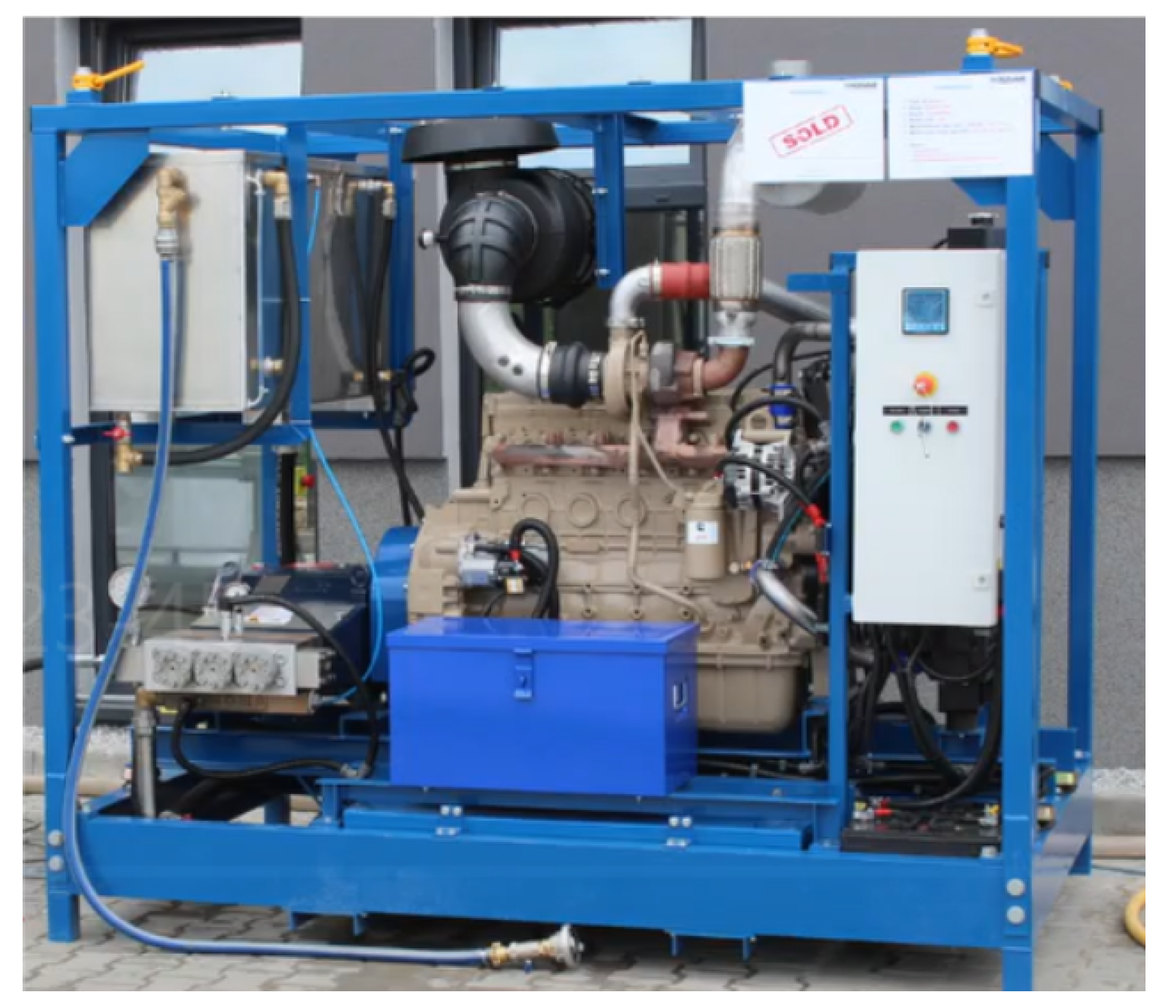
1.1. Hydraulic Power Unit Description

The object of this research was one of the high-pressure units manufactured for several years by PONAR Wadowice—the largest Polish manufacturer of hydraulic components and systems. This type of aggregate with a working pressure exceeding 1500 bar is used for the use of water as a tool, including for cleaning surfaces from rust or paint, cutting hard materials and drilling holes in them, and cleaning underwater surfaces of oil platforms from growths or cleaning tanks or deep wells. Aggregates of this type are equipped with diesel drives, which enable their mobile use in any place. Due to the use of ultra-high components, they work directly with water under this pressure, they are very expensive elements, and their possible failures affect the availability of the entire unit, and thus the entire process [11]. A photo of the hydraulic power unit that is the subject of a project is presented in Figure 1.

1.2. Business Needs

The industry of hydraulic components and systems (including high-pressure water systems) in recent years has experienced a very large development of new products that are currently used on the market. However, it should be mentioned that the dynamic development of hydraulic devices, such as HPU, is not possible indefinitely, as the pressures used today are sufficient for the current industrial applications to carry out most of the planned processes. Being aware of the above, the current portfolio of products and complete applications expands and develops solutions in the field of Industry 4.0, so that PONAR machines and devices are characterized by the highest possible availability, no uncontrolled downtime, and thus, savings and satisfaction on the part of the customer. The remote monitoring and predictive maintenance systems described in this article make the classic solutions in the field of power hydraulics “smart”, and introduce devices to the world of industry 4.0, thus building a competitive advantage. An important aspect to be mentioned is that the anomaly detection system presented in the article is not real-time. Nonetheless, a real-time system was not mandatory for the described project.

1.3. Literature Review

To compare the solutions developed in the article, a literature review is mandatory. The tools, concepts, and techniques that have been applied and described so far in the literature could be useful to point out the advantages and disadvantages of the presented approach. What is more, the examination of the state of the art allows for indicating innovations that this article brings into the domain.
More generally, not only related to hydraulic units, anomaly detection in industry was described in the survey by [12]. According to the categorization presented in that paper, the work within this article could be described as statistical/machine learning—constructive—point—online. In reference to the same survey, this project by application fits into the “machine condition monitoring” category of anomaly detection. An example of a case study involving a statistical anomaly detection method also described within the article is presented in the work [13]. The authors used the interquartile range (IQR) [2] method to determine anomalies for e-coating plants. IQR was considered a better tool than the Isolation Forest and Elliptic Envelope algorithms that were also taken into account. Many anomaly detection algorithms and use cases were mentioned and classified in the context of IoT in the publication [14]. According to the paper, sources of the anomaly could be, among others, errors and noise while collecting data and anomalous events during the operation of the device. The authors proposed grouping anomalies into three groups: point outliers, contextual outliers, and collective outliers.
Regarding the hydraulic domain, in the article [15], an online leakage detection system was developed that was also based on IQR value. The acquired 1-year monitoring datasets contain four gradual leakage events and two burst events. The presented results showed that the proposed method has successfully detected all leakage events with a short detection time and did not generate any false alarms in a year, which showed a promising future for this method.
The second modeling approach used in the paper involves black-box models, which are capable of capturing more complex dependencies in data; however, it is harder than in the case of the statistical approach to precisely describe in detail how output hypotheses were developed by the model. In the literature in an industrial context, HVAC devices were the subject of a research study presented in the publication [16]. The authors used the One Class SVM model with success to detect anomalies by first determining data from a device operating in nominal conditions. Afterwards, they changed the operating point and evaluated the learned model. The approach presented in [17] describes condition monitoring of complex hydraulic systems. The monitored elements were coolers, valves, internal pumps, and hydraulic accumulators. The Deep Neural Network (DNN) model was explained with the use of Deep SHapley Additive exPlanations (DeepSHAP) to determine what the most important factors that influence the final output of a model are. The accuracy metric that describes the quality of fault detection performed within the paper for monitored hydraulic elements were as follows: cooler-99.87%, valve-99.60%, internal pump leakage-99.09%, and stage flag (94.17%), with the exception of the hydraulic accumulator conditions (88.60%). Very good performance in terms of F1-score was achieved by the One Class SVM model presented in the same paper. The F1-score for the hydraulic system that was the subject of the research study was 99.68%. The anomaly detection approach developed for the hydraulic system was presented in the publication [18]. The dataset used within the paper comes from a real-world installation in Singapore. It emerged as a business need for research. In 2018, on a yearly basis, an average of 4.6 leak events per 100 km were reported. A model that is capable of signalizing anomaly 3 days before and localized with near 400 m accuracy with 80% F1-score has been developed. More than 3300 data-driven models were trained for optimizing the model performance to achieve the desired quality of modeling.
An anomaly detection system for HPU specifically was developed and presented in the paper [19]. The authors used several deep learning models such as the autoencoder, one-dimensional convolutional neural network, and long-short-term-memory network. The best model (1DCNN) achieved a distinction between normal data and data including anomalies with 94% accuracy in an industrial dataset enhanced with artificial anomalies.
In the context of the article, the use of expert knowledge for feature engineering is crucial. In the literature so far, the use of expert knowledge was applied successfully in the publication [20] for the spot welding process. In the described use case, the wear count threshold was set by domain experts, and this value determined the workflow of the anomaly detection algorithm. Another example of incorporating domain experts’ knowledge for feature engineering into industry was described in the article [21]. The subject of the article was a bitumen oven. As the authors stated, the description of the operating point and the ranking of the inputs were important for achieving satisfying quality in the models for predicting the surface temperature of the oven. The output of the model was used to enable the optimization of process parameters. However, in the literature, there is no described use of domain experts’ knowledge about hydraulic power units in the context of feature engineering for anomaly detection tasks, which is presented in this article.
The feature selection process, which is also part of the presented anomaly detection solution, was described in the literature using different approaches. One of the simple ones, which involves the Pearson Correlation Coefficient (PCC), was presented in the article [22] for the purpose of feature engineering of sensorized stamping presses. A use case closer to the subject of the herein article is presented in [23], where the authors used PCC to perform feature engineering for hydraulic components anomaly detection. There are also more complicated modern approaches involving neural networks. As an example of usage, autoencoders [24] or convolutional neural networks [25] could be provided. In addition, there is also the possibility of mixing together both PCC and neural networks in the feature engineering process as presented in the publication [26].
In the context of designing IoT solutions, in the publication [27], several trends and guidelines were provided. The authors mentioned that due to limited edge device resources, instead of implementing a whole TCP/IP stack based on the Open Systems Interconnection (OSI) model, a lightweight IP stack is normally implemented. Another important aspect to keep in mind while developing or projecting IoT solutions is the energy consumption of the device because that energy consumption primarily regulates the implementation of suitable protocols and standards in IoT devices. The study reveals that, in the context of security, Kumar et al. [28] proposed a lightweight encryption scheme that enables fast hash-keys-based encryption for IoT modules in the perception layer. The proposed scheme can mitigate security risks by only allowing communication between authenticated IoT devices.
Considering current issues and trends in the domain of anomaly detection for hydraulic power units, some open research problems can be named. Researchers try to explain black-box models so that the influence of input variables on the final output can be measured. The quality of the algorithms developed so far is very good. However, there are many more possibilities to combine existing algorithms, neural networks, and statistical approaches. Therefore, there is a broad area of research to create new algorithms that could obtain even better quality in anomaly detection and machine monitoring generally. Anomaly detection for hydraulic power units specifically is not a common research subject, so it could be explored much deeper. More often, as hydraulic systems, the smart water grid (SWG) is the subject of much research.

2. Materials and Methods

To implement the whole solution properly, a careful design has to be proposed. Within this section, the path from sensors through PLC and the edge computer to the cloud is presented. As the project was implemented in a production environment, aspects that are important from a business point of view, such as the costs of the solution and possible easy further solution propagation, were taken into consideration during development.

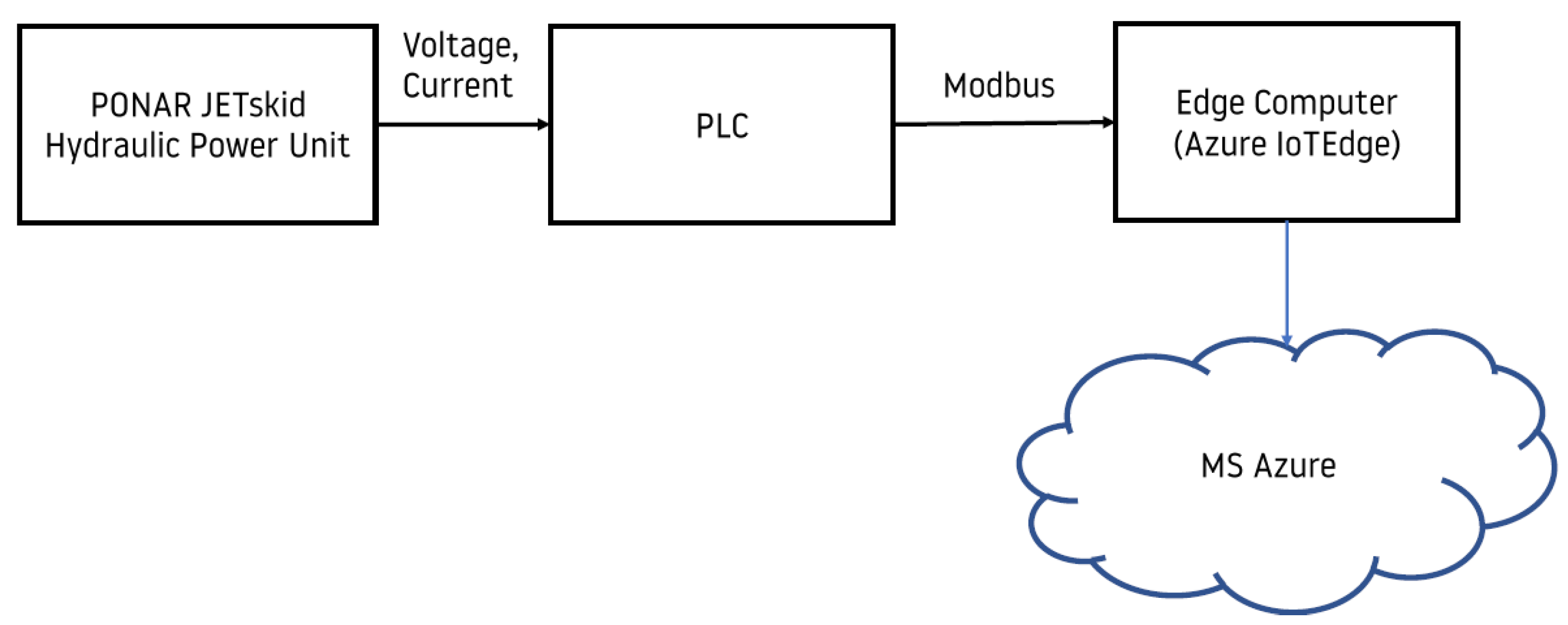
2.1. Data Acquisition and Communication

Good quality data is a fundamental principle to performing mature, useful, and reliable mechanisms for alarming, detecting, and predicting anomalies and failures. For that reason, the process of acquiring data from the very beginning, from the sensors layer, should be carefully designed.

2.1.1. Hardware and Software Architecture

All available measurements were aggregated in Siemens SIMATIC S7-400 [29] Programmable Logic Controller (PLC) acting as Modbus Slave. From proper input registers of the Modbus map, the following measured variables were available:
  • Pressure behind filter, bar;
  • Engine oil pressure, bar;
  • Fuel level, %;
  • Water level in the tank, %;
  • Fuel consumption, L;
  • Engine coolant temperature, °C;
  • Water temperature in the tank, °C;
  • Oil temperature, °C;
  • Power, W;
  • Rotation speed, 1 m i n ;
  • Oil flow, L m i n .
There are more variables available in PLC; however, they are diagnostics and binary quantities such as the presence of a sensor. Eventually, they are control-related variables such as set points. The SIMATIC S7-400 PLC unit can be considered relatively obsolete in comparison with, for example, S7-1200/1500, also manufactured by SIEMENS [30]. However, for practical and business reasons, there is no need to replace the PLC. Required functionalities such as the acquisition of signals from sensors and sharing measurements using the MODBUS protocol are ensured by the SIMATIC S7-400 unit. The replacement of the PLC would generate additional costs, require time for the PLC programmer, and also require taking HPU from the client for a while.
It would be possible to fulfill project requirements such as sending data to the cloud, and the use of anomaly detection algorithms using modern industrial software solutions, even compatible with SIEMENS, such as MindSphere [31]. However, using custom software implemented on the edge computer and in the cloud, rather than the use of out-of-the-box solutions, gives more flexibility in the context of further software and analytics development.
Software written in Python 3.8 was implemented to acquire data on the edge computer MOXA UC8100 [32] and send it to the cloud. Therefore, two functionalities were written:
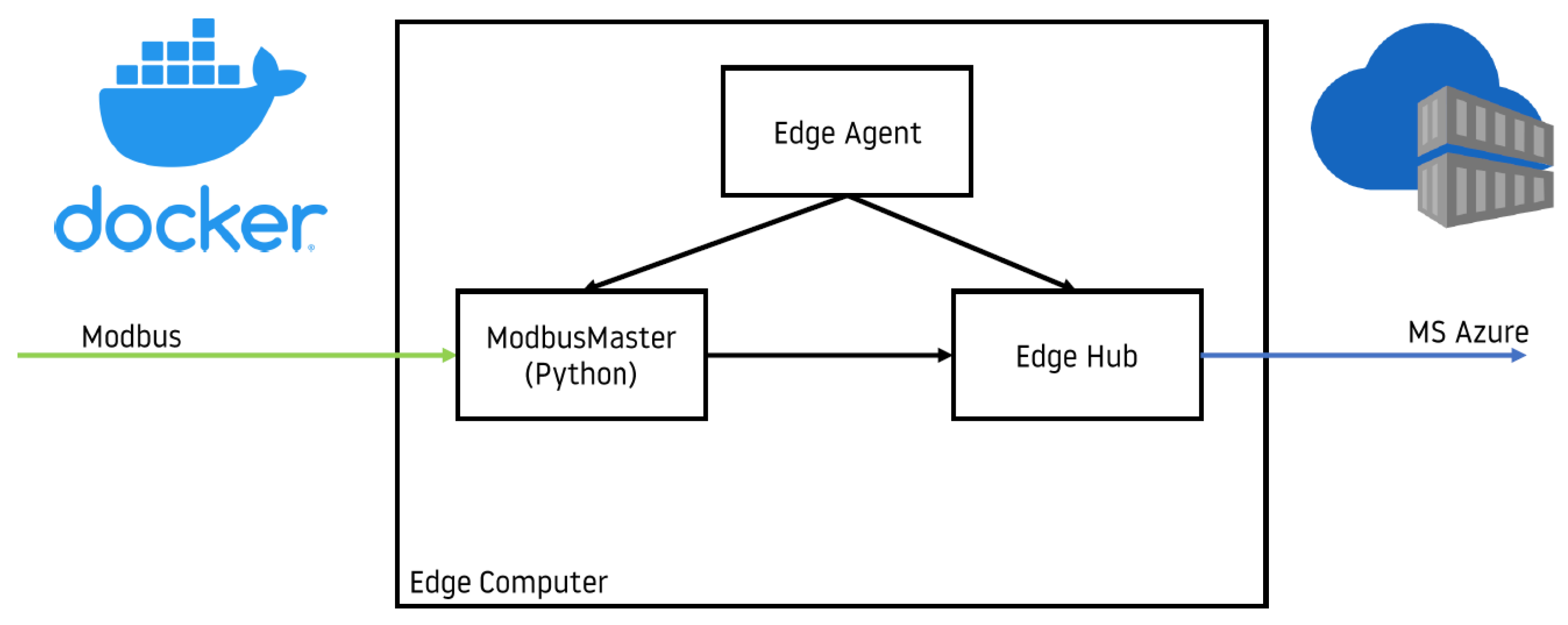
  • Reading data from Modbus (program acting as Modbus Master);
  • Sending data to the cloud in a proper format.
Thanks to software written on PLC, measurements were available through only one protocol—Modbus TCP. Only one program for data acquisition was necessary. The implementation of 1 involved the PyModbus Python package on BSD license [33]. Sending data to the cloud was performed using mechanisms available direct out-of-the-box from Python SDK for Azure IoT Edge [34] in the same program as Modbus Master.
The program fulfilling functionalities from points 1 and 2 has about 200 lines of code in total. The Pseudocode of the program is presented in Algorithm 1. Implementation in the development environment was performed as any other Python script. Deploying the solution into production is a bit more complex. Therefore, a separate paragraph (Section 2.1.2) for describing this process with the whole ecosystem around it is needed.
Algorithm 1 Program for reading measurements from PLC and sending them to the cloud
  • Require:  N = 11                 ▹ Number of measurement variables
  • t 1                              ▹ Time in seconds
  • X t x 1 , x 2 , x N              ▹ Vector of current measurement variables
  • X t 1 0 R N           ▹ Vector of previously read measurement variables
  • while True do
  •     if Connection with PLC is established then
  •         Read measurement variables from PLC and assign it to X t .
  •         if Value of any corresponding variable differs in X t and X t 1  then
  •            Send values of corresponding variables to the cloud.
  •         end if
  •          X t 1 X t
  •     else
  •         Try to establish connection with PLC
  •     end if
  •     Wait a second.
  •      t t + 1
  • end while
Figure 2 schematically shows the high-level solution architecture described above.

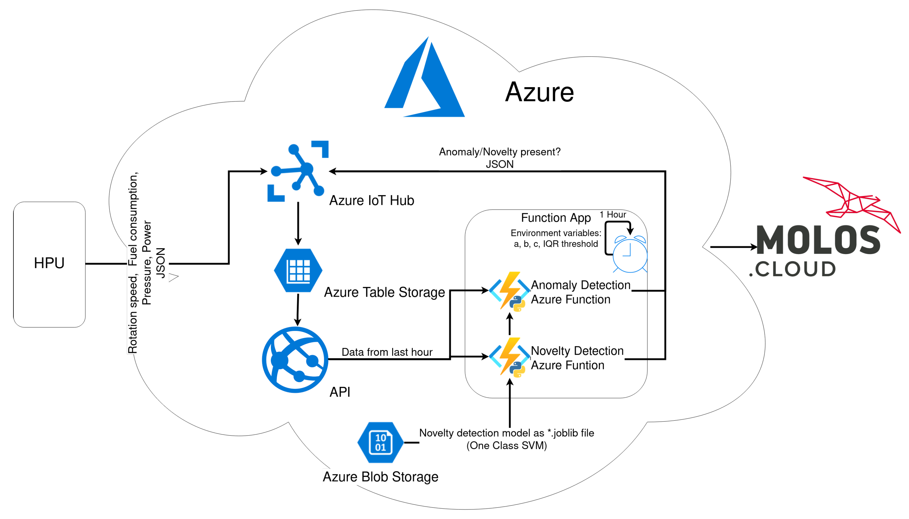
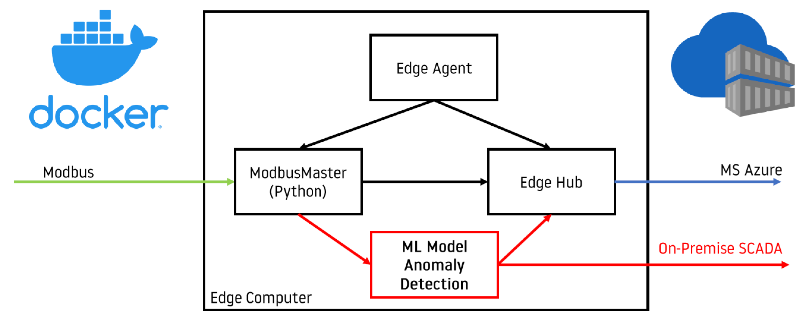
2.1.2. Azure IoT Edge

Azure IoT Edge [35] is a framework for developing and deploying edge solutions using Docker containers [36] that can communicate with each other. The core of IoT Edge architecture consists of two containers: Edge Agent and Edge Hub. The first container is responsible for handling and keeping an eye on all containers belonging to the solution. Whenever some container needs to be started, restarted, stopped, or updated, Edge Agent comes into play. Edge Hub is responsible for handling communication between containers with containers and containers with the cloud. Just like any other Docker container, containers within IoT Edge can fulfill desired functionalities by performing code inside the container. Containers are stored in a cloud container registry where they can be downloaded and uploaded. Deployment at scale is one of the most important features of Azure IoT Edge. Using this feature for purposes of anomaly detection for the HPUs project will be described in Section 5. A full description of Azure IoT Edge is presented on its official website [35].
On the edge computer, the Azure IoT Edge ecosystem was installed. With the dedicated software mentioned above (points 1 and 2), IoTEdge was responsible for acquiring measurements and sending them to Azure Cloud. Functionality is encapsulated in the Docker container.
A container can be thought of as a virtual machine but far more minimalist. It is an environment that provides all that is needed to run a program inside it. In the context of the described project, the Modbus Master container, visible in Figure 3, must have a Python interpreter with the PyModbus package installed and a minimal quasi-Linux operating system that is able to run the Python interpreter. It is important that the same container can be run on edge devices of different kinds, provided that they have the same CPU architecture and Docker environment installed.
The process of deploying containers on edge devices is carried out as follows:
  • Code development, including implementation of data acquisition presented in Algorithm 1;
  • Building Docker container;
  • Pushing Docker container to container registry;
  • Order container download to edge device via Azure CLI [37] or Portal Azure [38].
Programming within step 1 is performed in the same way as for a code that is not intended for containerization. This means that there are no additional techniques to be learned by the developer to provide a code that will also work within the container. The synthesis of the Docker container in step 2 requires a couple of specific Docker commands [39] and configuration files. As a result, a new Docker container appears, which is ready to be uploaded in step 3, for example, to Docker Hub [40] or Azure Container Registry [41]. The last step 4 ends the process of the deployment container on the edge device. Thanks to Edge Agent core-container, the just downloaded custom container starts automatically.

2.2. Algorithms Design

Before deploying algorithms into production, they should be carefully designed. The whole process begins with data preparation. Then, discovering key features that could be extracted from data takes place. Finally, a model that delivers value to the end user is developed.

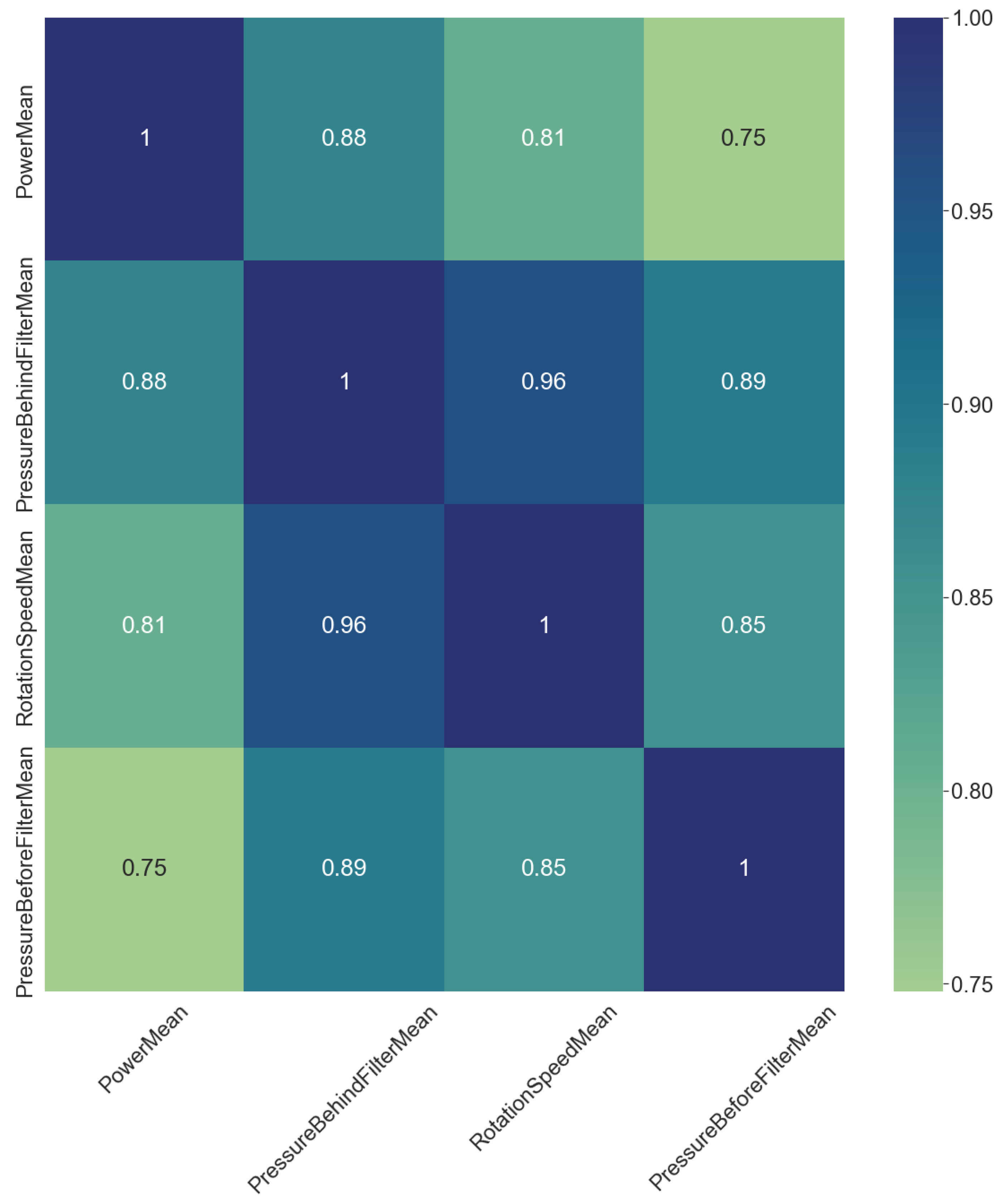
2.2.1. Feature Engineering

Consultations with domain experts (engineers from PONAR S.A.) give two potential features that could be useful:
  • Fuel consumption divided by power;
  • Rotation speed divided by pressure behind the filter.
According to the knowledge of domain experts from PONAR Wadowice S.A., both features are known to be positively correlated. However, consultations with experts did not provide mathematical equations that express both features. Only general insight was given. Therefore, Section 2.2.2 contains a description of the process of designing mathematical formulas that explain the relationship between variables within each of the features mentioned in the list in Section 2.2.1. The first feature is valuable from a business perspective because of the ability to monitor the exploitation process. The second in single value gives information on whether HPU works correctly—this means it gives output with proper quality.
It was decided to analyze only periods of stable work of the monitored device. Output pressure is a variable that determines whether some periods should be labeled as stable. Its course is analyzed to obtain information about stable periods. After labeling some time periods as stable, appropriate features from that period can be extracted. These features are mentioned in list in Section 2.2.1. The procedure of resolving stable periods using the GLR algorithm was described in [42]. There are other methods, such as the Iterative Algorithm for Time Series Decomposition into Trend and Seasonality presented in publication [43] or the Weighted CUSUM Algorithm [42] that are useful to resolve stable periods. Since programming the use of the GLR method was judged as easy during the implementation, we decided to use it in this method.
Such an approach is suited to detect abnormal behavior in the device operating point, where it is crucial to maintain proper and stable exploitation parameters. On the other hand, the approach proposed in the article as a whole is not useful to analyze transitions between operating points or on the hot/cold-start of HPU. The reason for this is that the proposed method of analysis assumes steady states of measured variables. For analysis of behavior during non-steady states, methods based on extreme value theory (EVT) [44] or DeepLSTM [45] are better suited.
Within each stable period, several basic statistics on measured data were calculated. These values are mean, median, standard deviation, 1st, and 3rd quartile. A couple of features were extracted. The next step will be to extract the most useful ones.
To verify the correctness of assumptions in accordance with expert knowledge, the Pearson correlation matrix [46] was constructed. Correlating all values with each other resulted in approximately 200 characteristics. Then, characteristics were filtered to take only several correlations that have the highest absolute value of the Pearson correlation coefficient (PCC). The correlation matrix with the most significant correlation pairs is shown in Figure 4. It is worth mentioning that only positive Pearson correlation coefficients are significant.
Fuel consumption with respect to power has the highest correlation coefficient. Pressure behind the filter due to pressure before the filter has the second highest value. However, according to domain experts’ knowledge, it does not represent any physical phenomena. The third highest PCC value has a rotation speed mean with respect to pressure behind the filter. Therefore, both characteristics proposed by domain experts in the list in Section 2.2.1 are taken into consideration in the next steps of modeling.

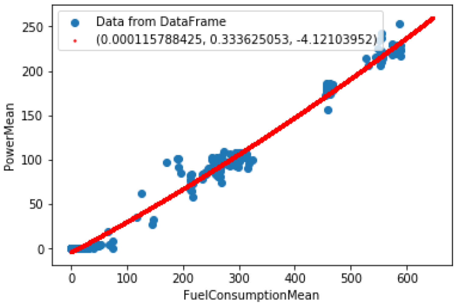
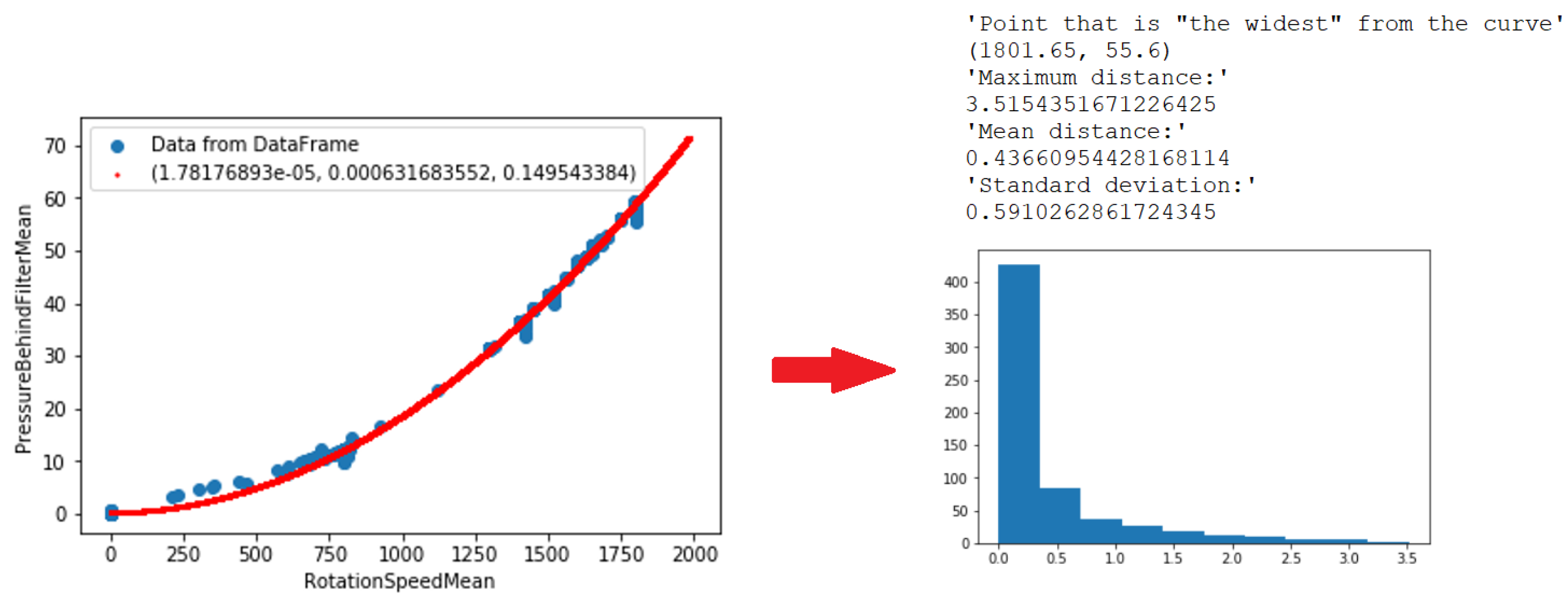
2.2.2. Fitting to Characteristics

The features proposed in Section 2.2.1 should be somehow handled to give value. Plotting them on scatter-plots (Figure 5 and Figure 6) shows that some reference curves can be fit. The shape of characteristics seems to be simple to determine. Then, it was decided to use a simple tool—linear regression from Python NumPy package [47]. An explanation of linear regression principles is beyond the scope of this article but can be found at [48].
Two characteristics were fit:
  • Power mean due to fuel consumption mean;
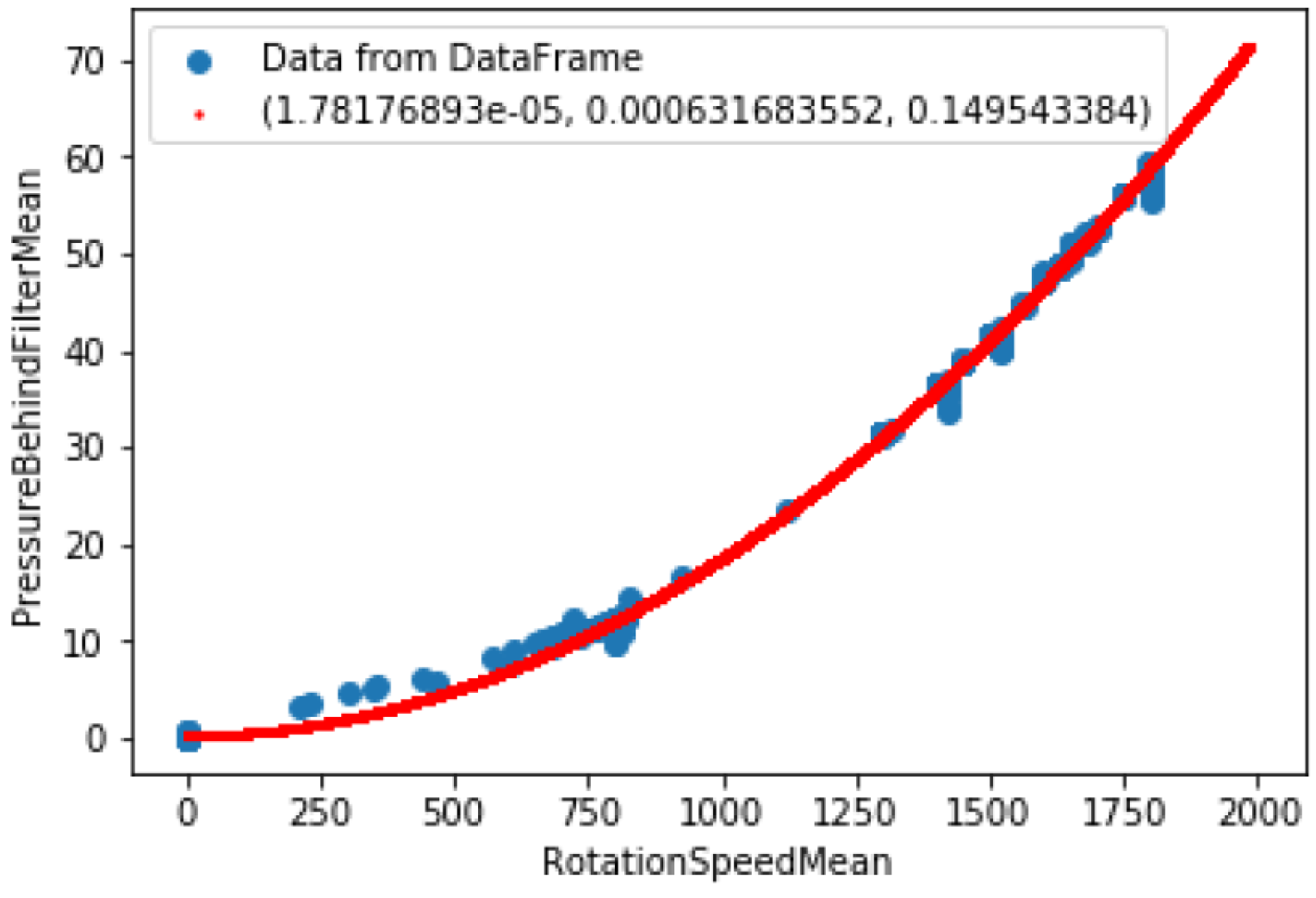
  • Pressure behind filter mean due to rotation speed mean.

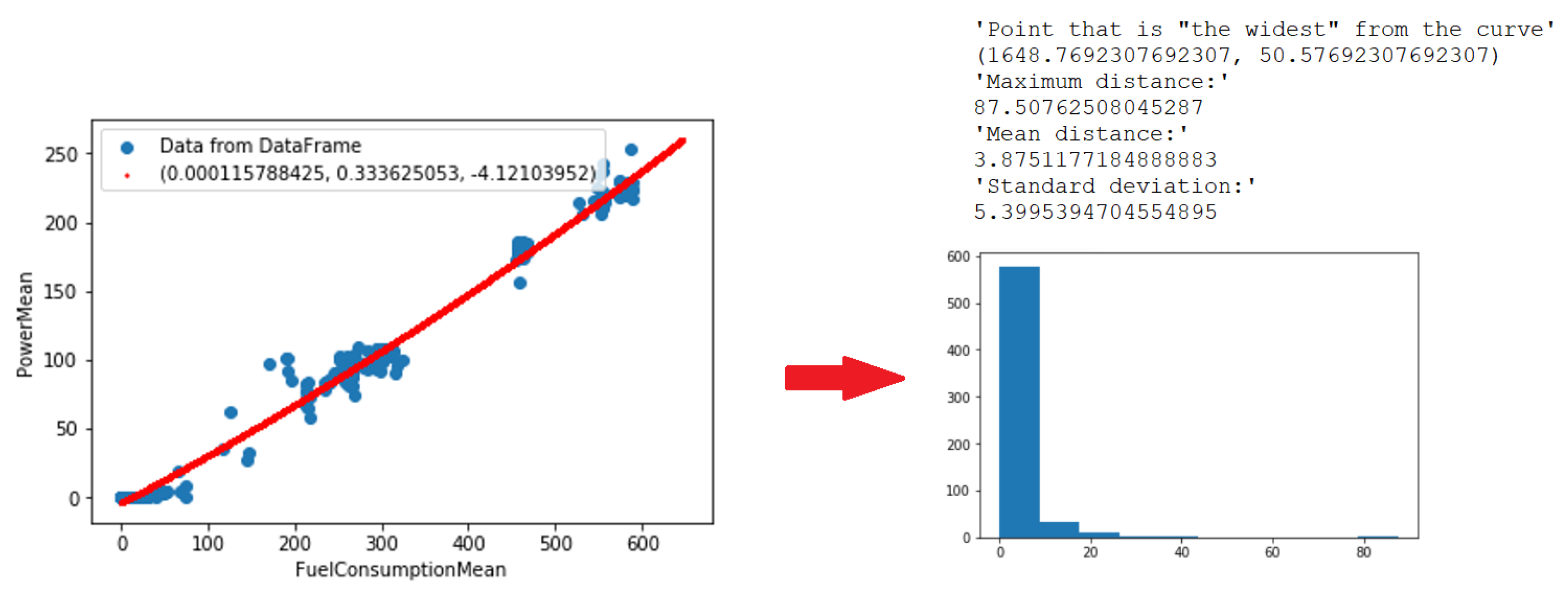
2.2.3. Anomaly Detection

After establishing reference curves, the anomaly detection algorithm comes into play. The chosen approach involves an examination of deviations from reference characteristics. The process of finding the point-to-curve distance (PTCD) is described in [3]. The approach assumes the curve as a closed-form expression, which is the case presented in Section 2.2.2. Firstly, the distance from the curve to new measurements put on characteristics is calculated. Secondly, a histogram of distances from the curve is established. The last step is to identify outliers. To identify them, it was decided to use the Interquartile Range (IQR) Criterion [2].
Concise mathematical use of the IQR Criterion could be presented as follows. Firstly, IQR is calculated as presented in Equation (1).
I Q R = Q 3 Q 1
where Q 3 denotes the third quartile (75th percentile) and Q 1 denotes the first quartile (25th percentile) of all acquired PTCD values for each characteristic separately. For each characteristic separately, any PTCD value denoted as P T C D i that meets the condition presented in Equation (2) is considered as abnormal.
P T C D i > Q 3 + 1.5 I Q R
While using IQR Criterion, values that also meet the condition presented in Equation (3) are considered abnormal. However, for the case analyzed in this study, the wider the point is from the reference curve, the more suspicious it is to be considered as an anomaly. Therefore, to determine if a point on characteristics is considered an anomaly, only the condition from Equation (2) is applied in the article.
P T C D i < Q 1 1.5 I Q R
There are more anomaly detection algorithms available, such as those based on autoencoders [49] or SVM [50]. However, PTCD with IQR Criterion was applied in this study because it was considered as easy enough to interpret by domain experts from PONAR Wadowice. For now, it is not possible to change anomaly detection algorithms because the solution was deployed into production and HPU works with the client.
Variables used within the anomaly detection algorithm were proposed by domain experts from PONAR Wadowice based on their experience. The choice of the variables was also supported by correlation analysis performed in Section 2.2.1. These variables are power, pressure, fuel consumption, and rotation speed. Other variables, such as temperature or fluid level, can help increase the accuracy of anomaly detection; however, other variables were taken into the final algorithm design based on domain experts’ experience. The range of variables that are used by the anomaly detection algorithm could not be performed and implemented because the solution is currently deployed in production. The use of other variables than those chosen so far for the anomaly detection algorithm could be carried out while deploying the algorithm solution on the next HPU.

2.2.4. Novelty Detection

After implementing the approach described in Section 2.2.3, another was proposed and developed. The goal was to analyze data in higher dimensional space. Therefore, some black-box or gray-box algorithms could be used as they are capable of drawing conclusions from high dimensional data much more efficiently than by-hand analysis. The assumption was performed that all data we take into account in this approach are non-anomalies. Then, instead of anomaly detection, the task was novelty detection [51]. It was decided to use One Class SVM (OCSVM) [4] because it is easy to deploy with the scikit-learn Python package [52].
The principles of the OCSVM algorithm are as follows [53]. The training process involved taking only data that come from standard HPU working conditions according to the knowledge of domain experts from PONAR Wadowice. Therefore, we let the dataset of normal samples be:
X = [ x 1 , x 2 , , x n ] T R N x L
and the target decision hyperplane be:
f ( x ) = ω ϕ ( x ) ρ = 0
Afterwards, the optimization problem could be constructed and solved:
min ω F , ξ R N , ρ R 1 2 | | ω | | 2 + 1 N v i = 1 N ξ i ρ
s . t . ω ϕ ( x i ) ρ ξ i , ξ i 0
where:
  • N is the length of the dataset used for training;
  • v is the regularization parameter;
  • ξ i is the slack variable corresponding to each dataset;
  • ω and ρ are the decision planes that can be decided with participation;
  • ϕ denotes the way the data are spatially mapped [54].
The OCSVM model is obtained by introducing Lagrange multipliers α i 0 and β i 0 and solving the Lagrange equations.
L ( ω , ξ . ρ , α , β ) = 1 2 | | ω | | 2 + 1 N v i = 1 N ξ i ρ i = 1 N α i [ ω ϕ ( x i ) ρ + ξ i ] i = 1 N β i ξ i
Partial differentiation of the variables in the above equations gives the pairwise form of the optimization problem [55]:
min α α T H α
s . t . α i 1 N v , i = 1 N α i = 1
where H denotes the kernel matrix, the components of which are H i j , which can be expressed as:
H i j = K ( x i , x j ) = ϕ ( x i ) ϕ ( x j )
where K ( x i , x j ) denotes the kernel function, that for the purpose of the article is the Gaussian kernel function. As for the RBF kernel function, only one parameter, denoted as σ , is to be adjusted. This parameter directly affects the width of the RBF kernel function, and the calculation formula is presented in Equation (12).
K ( x i , x j ) = exp | | x i x j | | 2 2 σ 2
The quadratic problem that is stated above leads to solving α , whereupon ω and ρ can be computed separately as presented in Equations (13) and (14)
ω = i = 1 N α i ϕ ( x i )
ρ = j = 1 N α j K ( x i , x j )
As a result, a decisional hyperplane in the feature space can be found from the solved ω and ϕ .
The decision function that is defined in Equation (15) is established for classifying the test sample z k from the training set Z = [ z 1 , z 2 , , z M ] T R M x L .
F ( z k ) = s i g n [ ω ϕ ( z k ) ρ ]
The sample is classified as a normal sample when the value of the decision function is positive, so when F ( z k ) = + 1 . When the value of the decision function is negative, i.e., when F ( z k ) = 1 , the sample is classified as an abnormal sample because it falls outside the decision hyperplane.
It was decided to take the following variables as input to the algorithm:
  • PressureBehindFilterMean;
  • HighPressureMean;
  • RotationSpeedMean;
  • PressureBeforeFilterMean.
The choice was dictated by the same logic as described in Section 2.2.1. These variables have the highest PCC in all available pairs of variables in the solution. Therefore, they tend to form not-so-dispersed shapes (cloud of points) in high-dimensional space.
Naturally, more variables could be taken into consideration as an input into algorithm. For example, temperature or fluid level. However, the fewer variables the model has, the easier it is usually to interpret. In the described project for domain experts, it was crucial to understand the behavior of HPU as tangible as possible and to make the novelty detection model as easy to interpret as possible for the domain experts from PONAR Wadowice. The possibility of expanding the range of variables could be considered during deploying the presented solution on the next HPU. For now, the solution is deployed in production and there is no possibility of its modification.

2.3. Algorithms Deployment

After developing models that are useful and give value to the end user, it is time to make them work in a production environment. Data are stored in Microsoft Azure Cloud as described in Section 2.1. To provide an ecosystem for models that is maintenance-free and convenient in implementation, it was decided to use Microsoft Azure Cloud. Using such an approach, it is possible to deliver value from models to the end user.
According to Figure 7, the architecture of cloud services does not involve only analytical tools per se. It also contains API that is used for acquiring data from cloud storage. In addition, it contains MOLOS.CLOUD web SCADA by REDNT S.A., where the end user can see measurements and alarms emerging from developed analytical hypotheses.
The core of the system is Azure Functions [56] paired with analytical models. As described in Section 2.2, two approaches have been developed. Each approach has a different method of deployment. However, they are embedded in the cloud in the same way.
Embedding algorithms in the cloud involves Microsoft Azure Functions. This cloud service allows us to run programs and scripts written in JavaScript, C#, F#, Java, PowerShell, Python, and TypeScript in the cloud, i.e., serverless [57]. The code developed within the project was written in Python, so the language was supported by Microsoft Azure Functions. For project purposes, the execution of functions was scheduled. However, it is not the only mechanism to trigger the execution of the Azure Function [58]. Each developed algorithm has its own timer-triggered Azure Function that is executed once an hour. Therefore, two Azure Functions were developed in total.

2.3.1. Anomaly Detection

The goal of deployment is to perform calculations hourly to provide information about anomalies. The developed approach involves a reference curve described by three parameters per characteristic and an error threshold per characteristic. Such a set of parameters enables us to check whether, in the monitored time period, the anomaly has appeared. Such a functionality could be implemented with Azure Functions.
Azure Functions are part of the Azure Function App, which is an environment for Azure Functions execution. This environment has its own environment variables that can be accessed by Azure Functions inside it. The parameters required to work out the anomaly detection hypothesis are:
  • a, b, c—coefficients for Equation (16). Two sets of parameters, because of two fitted characteristics;
  • Interquartile Range (IQR) criterion mentioned in Section 2.2.3. Two parameters, one per each characteristics.
In total, the Function App had to store eight parameters, which is a complete set to run Azure Function for anomaly detection. All these parameters are declared as Function App environment variables.
The parameters of the algorithm could be accessed from other sources such as Azure BLOB Storage or Table Storage. For simplicity of implementation, it was decided to place them inside the Function App. In this way, it is easy to change them on the spot without modification of the Azure Function code, which is important from a long-term maintenance perspective.
Finally, the algorithm should deliver value to the end user. For fulfilling this requirement, after developing hypotheses, feedback to the IoTHub in the form of a JSON message is provided. The message contains information on whether an anomaly has occurred, with specifications on from which characteristics the anomaly has emerged. Moreover, the “intensity” of the anomaly is sent to IoTHub. The message after processing is put with its content into Azure Table Storage. Then, MOLOS.CLOUD web SCADA is able to extract data from Table Storage and show alarms about anomalies if necessary. In the end, the end user is aware of occurring anomalies.

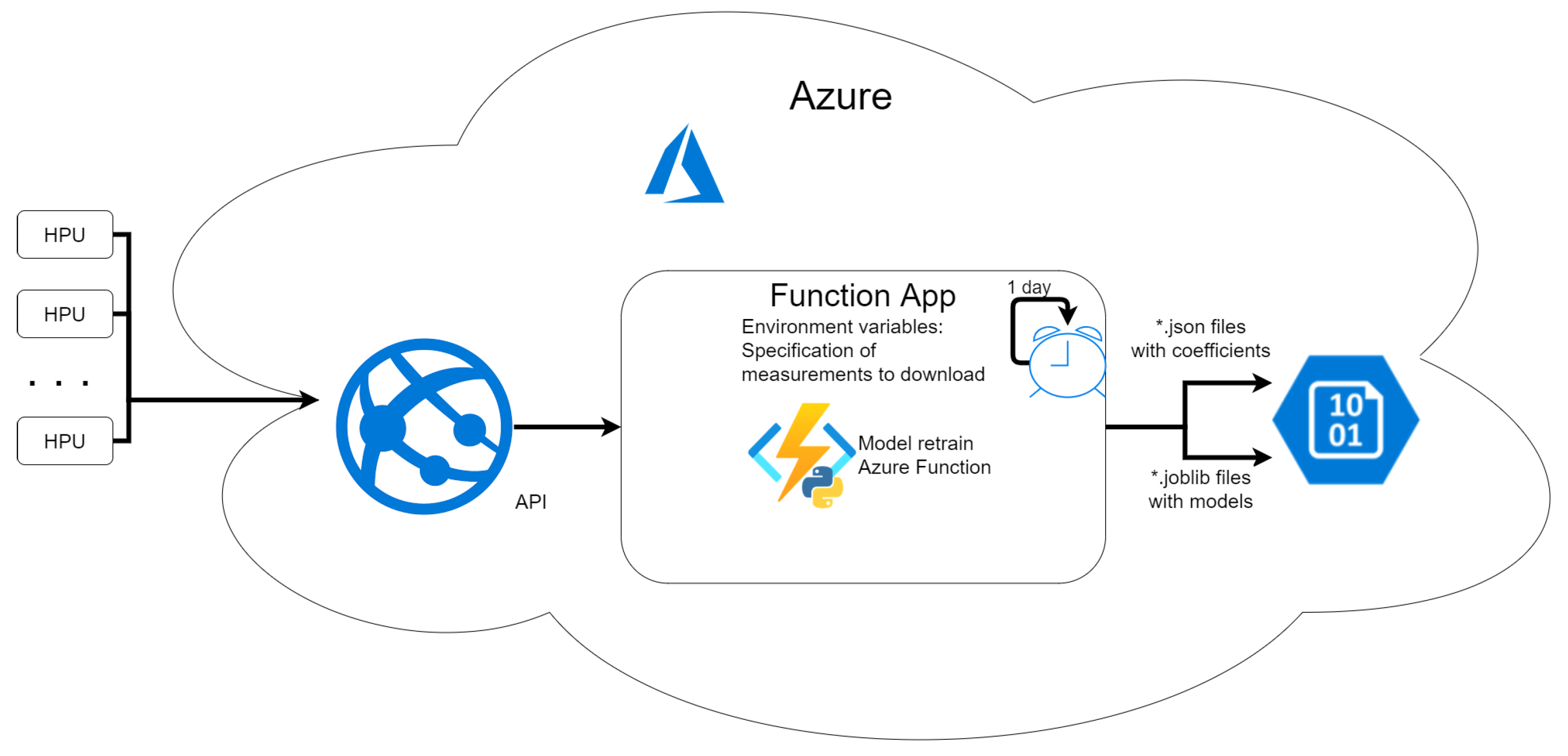
2.3.2. Novelty Detection

The novelty detection algorithm runs once an hour inside the timer-triggered Azure Function. The mechanism that decides whether novelty has been detected is the One Class SVM model trained in Section 2.2.4. After training the model, it is exported as a *.joblib file, and inside the Azure Function model, it is imported and used. This is common practice while dealing with scikit-learn models [59]. Finally, the model tries to find novelty in delivered data.
Similarly to Section 2.3.1, for the novelty detection case, a message to IoTHub is also sent. The message contains information on whether novelty has been detected or not.

2.3.3. Tests Performed before the Solution Was Deployed in Production

Deployment of both code and models were preceded by tests. The testing code was performed on a dedicated experimental measurement station in the REDNT S.A. office. The station included the same model of edge computer (MOXA UC-8100) as on the hydraulic power unit. Due to the lack of SIMATIC S7-400 PLC in the office, Modbus Slave was simulated by Modbus Slave software [60] during tests on a test stand in the office. The register map was simulated according to the map that was implemented on PLC on the hydraulic power unit. Testing the code involved manual tests that were carried out by changing the values of the registers with the same addresses and same variable types as variables stored on destination PLC on HPU. From a functional point of view, it is not a problem that Modbus Slave software was used for tests in the office instead of SIMATIC S7-400 PLC. The communication interface, register map, and register data types were replicated as it was on HPU with PLC. There was no possibility of performing manual testing on destination installation stated in Section 2.1.1 because PONAR Wadowice conducted other activities to prepare the HPU for shipment to the customer. Therefore, a carefully designed testing environment was needed in the office.
The procedure of manual testing of the data acquisition process was designed with consultations with domain experts from PONAR Wadowice S.A. They provided ranges of values that are possible when HPU is in an acceptable working state. The testing experiments consisted of manually changing values of registers that correspond to variables in the Modbus register map within acceptable ranges provided by domain experts.
During testing, it emerged that the register that held the power measurement Section 2.1.1 was 16-bit, but for values of power that were beyond this range it needed a 32-bit register. Therefore, to avoid incorrect measurement values, changes in PLC software in production were required.
After performing manual tests of data acquisition software on the simulated environment and ensuring that data acquisition software is written without bugs, tests on destination installation mentioned in Section 2.1.1 were carried out. The aim of the testing was to change the operating point by decreasing and increasing the value of output pressure. Both changes that are within an acceptable working regime and beyond it were performed. After performing test scenarios on HPU and checking that data were properly acquired, models and algorithms were trained. After training, models were tested using data from test scenarios performed on HPU to ensure that they will not raise anomalies within an acceptable working regime. Testing of the models was carried out by manually putting data from different operating points on the input of the models. These operating points were picked with consultations with domain experts from PONAR Wadowice to help consider whether test input data should be considered as an anomaly. In total, four tests were performed. All tests were carried out during one workday. Each of the tests lasted one hour. Unfortunately, there was no possibility to perform extensive tests because the hydraulic power unit was dedicated to concrete commercial projects, not for research purposes only. Therefore, a limited amount of time and human resources from both REDNT S.A. and PONAR Wadowice S.A. could be provided for the research. The simulation data are not suitable for training because the simulator did not properly reproduce the behavior of the actual HPU. The simulator was created only for the purpose of verifying the data acquisition software and checking the reference ranges and pre-preparing the data processing pipeline for training. It did not cover the relationships between variables, nor did it take into account the dynamics of changes in variables. It only allowed changes in individual variables listed in the list in Section 2.1.1.

2.3.4. Summary of Algorithms Workflow in Production Environment

To summarize Section 2.3.1 and Section 2.3.2, step by step, the deployed algorithm runs as follows:
  • Download required variables time series (power, pressure, fuel consumption, rotation speed) from cloud storage using API from the last hour.
  • Determine stable periods.
  • Calculate mean for each variable for each stable period.
  • Handle anomaly detection:
    (a)
    Calculate point-to-curve distance (PTCD);
    (b)
    Confront PTCD with IQR Criterion.
  • Handle novelty detection:
    (a)
    Download model from BLOB storage;
    (b)
    Use model to predict novelty.
  • Send feedback to IoTHub on whether an anomaly or novelty was detected or not. MOLOS.CLOUD will raise an alarm if necessary.
It is worth mentioning the costs of deployed workflow and ecosystem for analytical solutions. Several components that generate cost could be named:
  • Function App as a consumption plan [61]:
    • Costs are generated per Azure Function run;
    • In described solution it is 2 f u n c t i o n s 24 e x e c u t i o n s d a y f u n c t i o n 30 d a y m o n t h = 1440 e x e c u t i o n s m o n t h .
  • Storage:
    • Costs are generated by read operations—both volume and quantity of reads;
    • Read operations from table storage with time series data for desired variables;
    • Read operations BLOB storage with models for anomaly detection;
    • Read operations BLOB storage with models for novelty detection.
  • API:
    • Fee is charged for working hour.
The approximate cost of Azure cloud resources for data analysis in the described project is about EUR 10 per month. The costs were calculated based on invoices received from Microsoft. Unfortunately, the costs of specific components pointed out in the list in Section 2.3.4 were restricted and could not be provided in the article. In the context of project cloud costs, it is also possible to use the Azure Pricing Calculator; however, it gives only a rough estimate of costs. An accurate cost calculation using only the Azure Pricing Calculator is hard because making assumptions about data of inbound and outbound traffic in the cloud is hard to be carried out accurately and often requires the usage of special traffic monitoring tools [62]. Moreover, the proper interpretation of calculations made using the Azure Pricing Calculator is often hard [63]. Therefore, a common experience is that accurate costs of cloud resources are known only after deploying the solution.
It is important to notice that the solution is not real-time monitoring. Hypotheses are developed once an hour. Assumptions made during the synthesis of Azure Architecture have not involved real-time workflow. Therefore, the used cloud tools are not suited for such a workflow. For a fast and responsive tool for monitoring in Azure, see Azure Stream Analytics [64]. Moreover, to estimate the cost of the whole delivered Azure solution (visualization + analytics) to the above costs, a couple of other components should be added. Nevertheless, it is beyond the scope of this article because the description of visualization details in both a frontend and backend manner is not the purpose of the article.
A concise summary of workflow and tools used while putting algorithms into production is shown in Figure 7.

2.4. Cyber Security

As every software solution requires connecting to the internet and using interfaces to interact and communicate with other devices, the described solution could also be vulnerable to cyber attacks. However, several security tools, concepts, and mechanisms were applied to ensure safety on a high level. First of all, firewall rules on the edge device, MOXA UC-8100, were applied. Whole inbound network traffic was blocked and then gradually opened for appropriate ports and IP addresses. IP addresses of Azure servers are known [65]. The number of ports through which communication with the cloud takes place is also known (8883-MQTT). Therefore, proper firewall rules could be applied. The connection with Azure IoTHub is secured using TLS/SSL. A comprehensive description of communication details related to IoTHub could be found in Microsoft documentation [66]. MOXA UC-8100 also communicates with PLC using the Modbus TCP protocol. The IP addresses of PLC and Modbus TCP port (502) are known, so another suitable firewall rule could be written. Nevertheless, the described actions were taken to improve security and minimize the risk of security incidents.

3. Results

Each of the approaches stated in Section 2.2 delivered results that were part of the final solution. The results will be described and compared with other similar use cases from the literature.

3.1. Anomaly Detection

With the use of the NumPy package, the curve fitting procedure was carried out. Based on the shape of characteristics in Figure 5 and Figure 6, linear, quadratic, and exponential functions were taken into consideration as reference curves. In the results, it arises that the optimal curve that explains both characteristics are quadratic. The standard form of the quadratic function was used to fit the reference curves:
f ( x ) = a x 2 + b x + c
where:
  • a, b, c are functions coefficients that are real numbers.
The values of determined coefficients for each of the considered characteristics are presented in Table 1. The coefficient a for the characteristic from Figure 5 and coefficient b for the characteristic from Figure 6 have low values. They could be eliminated after applying some regularization, for instance, L1 or L2 [67]. However, characteristics are fit using only data from the proper behavior of HPU. Therefore, they were not necessary to eliminate negligible coefficients.
According to the approach described in Section 2.2.3, threshold values that are necessary for deciding whether measurements are anomalous or not were computed. Based on the error distribution that is presented in Figure 8 and Figure 9 and the application of IQR Criterion, threshold values were evaluated. The values are presented in Table 2.
In the current phase of the project, detected anomalies are consulted on an ongoing basis with domain experts from PONAR Wadowice S.A. An assessment of the results and quality of the developed solution in production is in progress.

3.2. Novelty Detection

The One Class SVM algorithm was trained using standard parameters defined in the scikit-learn package [52]. As kernel type, the Radial Basis Function (RBF) was used. The kernel coefficient was set to scale, so it was dependent on the number of features and their variance. The coefficient related to the upper bound on the fraction of training errors and the lower bound of the fraction of support vectors (called nu) was set to 1 because the novelty detection algorithm was trained entirely on only non-anomalous data. Similarly to anomaly detection results presented in Section 3.1, so far, anomalies detected during the project are consulted on an ongoing basis with domain experts from PONAR Wadowice S.A. The solution undergoes evaluation in production.

4. Discussion

4.1. Algorithms

Both anomaly and novelty detection approaches could be useful in the context of determining whether HPU working parameters become anomalous. The results related to anomaly detection presented in Section 3.1 show that the use of selected reference characteristics is justified. PCC values for the characteristics and quality of fitted curves are good enough to make assumptions that are starting points for picking anomaly detection criteria. An industrial example of an anomaly detection system that also selects inputs to the model with the use of PCC values is presented in [68]. The authors claim that the use of PCC to select inputs to the model improved the accuracy of the presented system even if PCC has limitations as it is only sensitive to the linear relationship between variables. The use of the IQR Criterion applied to the distribution of distances from points on characteristics that come from measurements to reference curves results in the determination of clear and understandable threshold values. When the distance of data points from measurements exceeds these values an anomaly is signaled. Such an approach could be presented and explained to a non-expert person from the client side, which is also a plus in the context of the described project. Incorporating IQR Criterion into anomaly detection algorithms on industrial datasets presented in the study [69] shows that fewer false positive alarms are raised in comparison to other techniques used in the paper such as Isolation Forest or Elliptic Envelope. On most of the datasets considered in the study, the precision score of the algorithm with IQR Criterion applied was significantly better (best value 0.6) than for Isolation Forest (best value 0.16) or Elliptic Envelope (best value 0.2). More modern algorithms such as autoencoders in combination with LSTM or CNN networks are effective real-world hydraulic solutions [70]. The presented approach allowed us to detect anomalies 2.5 h before failure occurred. Being aware of method limitations and the possibility of using more modern techniques, after consultations with domain experts from PONAR Wadowice, it was decided to implement PTCD with the IQR Criterion algorithm because of its simplicity accepting that the algorithm could potentially be of a lower quality than the aforementioned.
Novelty detection described in Section 2.2.4 involves a One Class SVM model, which is a kind of black-box. This model is less explainable than the threshold-based approach within the anomaly detection approach. Consulting anomalies detected using this approach with domain experts is therefore harder. Due to the ability of OCSVM to analyze data having more dimensions than the approach involving IQR Criterion, OCSVM is able to potentially capture anomalies of different kinds to anomalies detected by the approach involving IQR Criterion. As a method that is easy to implement in Python using the scikit-learn package, we decided to implement OCSVM. It was presented in the article [71] that, using hyperparameters tuning (manual search, grid search, random search, and Bayesian optimization), the quality of the algorithm could be improved. The worst F1 score equal to 0.55521 was obtained by manual search, and the best F1 equal to 0.6488 was obtained for Bayesian optimization hyperparameter tuning. For the purpose of the presented case study, the OCSVM algorithm has default hyperparameter values, and no tuning was performed. As a recent anomaly detection algorithm with a high F1 score equal to 79%, the Graph and Temporal Neural Network for Multivariate Time Series Anomaly Detection (GTAD) presented in paper [72] could be pointed out. Therefore, when revisiting the solution, investing time in tuning hyperparameters or even changing the algorithm is worth considering.
Use cases of commercially implemented anomaly detection systems for hydraulic systems were described in papers [73,74]. However, they do not involve integration with Microsoft Azure Cloud and IoTEdge technology specifically. Paper [75] describes a framework for data capturing and processing in the cloud but without Azure IoT Edge technology. Therefore, the literature lacks publications that characterize commercial systems for anomaly detection for hydraulic power units with the use of Azure cloud and Azure IoT Edge.
The results obtained in the article are specific to the monitored device. However, as described in paper [76], IQR Criterion is proved to be useful in the context of detecting anomalies in the automotive industry. On the other hand, as presented in paper [77], regression could be useful in the context of outlier detection. Therefore, a fusion of these approaches presented in the article has the potential to give reasonable quality of anomaly detection system. The novelty detection algorithm involving One Class SVM presented in the article was commonly applied in industry as presented in papers [78,79]. Therefore, it is reasonable to pick this algorithm for a system developed during the described project.
The evaluation of algorithms in production is in progress and due to formal business determinants presenting detailed results is not allowed so far.

4.2. Solution Limitations

Potential limitations of the presented solution that are related to connectivity, data quality, and algorithm quality could be discussed. As HPU is the device that is a standalone mobile device, it has many potential locations where it can work. Therefore, some connectivity issues could arise. The most possible one is that no internet access will be available in the place where HPU operates. Hardware, for instance, the network card or antenna in MOXA UC-8100, also could be damaged. Azure IoT Edge, the technology used within the solution, is capable of storing data that should be sent to the cloud when the device has not got internet access. Data are stored on the edge computer hard disc, so in case of problems with the power supply, data will not be lost. As data are stored on a hard disk, its volume is an important aspect to mention. MOXA UC-8100 has 8GB eMMC storage in total. After installing the operating system, software, libraries, and packages that are required for the whole solution to work properly on the edge computer, there is almost 5GB of space left on the device. This is enough to store approximately one month of measurements with selected acquisition parameters and variable range. It is possible to use an SD card as external storage in MOXA UC-8100. However, data stored on a hard disk is safer than stored on an SD card, even if such a card is industrial grade.
Even if the edge computer is capable of storing enough measurements to ensure that lack of internet access is not a problem in a broad time horizon, there could emerge connectivity issues between the edge computer and PLC. For the period when the connection is broken, data are lost. There is a gap in data that cannot be filled. The connection from sensors to the PLC input module also has the possibility of being interrupted. In such a case, there not will be a gap in data, but the quality of acquired measurements is poor. Corner cases that could emerge in such a situation are handled. There are registers in PLC that store information about the presence of the sensors. Input data to anomaly detection algorithms are filtered in a simple way by applying a threshold on data. Justification for such an approach is a known issue related to a range of sensor indications when, in case of its failure, the sensor outputs a minimal or maximal analog value that corresponds to too large or too small indications. Corrupted data from two corner cases described above is therefore not considered for further analysis. However, there is no mechanism implemented that ensures all issues with sensors that could emerge. Therefore, data corruption, however unlikely, is always possible even if measurements do not seem suspicious. To address potential problems with reading from sensors, in the literature in the paper [80], the algorithm related to machine condition monitoring that takes data from malfunctioning sensors into account is presented. Another interesting example was presented in the publication [81], where the authors developed an algorithm called the adjacent information recovery (AIR) filter, which handles incomplete data issues in fault detection systems. The mentioned methods solve a variety of issues with incomplete data; however, the adaptation of the above algorithms into the solution presented in this article will consume time that, at this stage of a project, is not available.
Models tests that were carried out during algorithm development helped to train and tune algorithms in a way that they did not raise useless alarms (false positives) or that algorithms missed alarms (false negatives). The amount of data from tests is not sufficient to cover all possible conditions and working regimes of HPU. For sustainable industry, as stated in the publication [82], both alerting on the most severe anomalies and minimizing false positives are critical. From that point of view, the number of false negatives increases; however, this is a common compromise for anomaly detection tasks in industrial applications [83]. To address this aspect, in the article [82], it was proposed that raising the alarm should occur when the number of consecutive anomalies detected by the algorithm is higher than a specific number determined by the experts. To address this aspect more data should be acquired to be more aware of device operating points, and then after revisiting the solution, suggesting an approach involving raising an alarm after more than one detected anomaly should be considered. For now, it is not possible to present how many false positives or false negatives algorithms raised. Accessing quality of anomaly detection algorithms could be performed after revisiting solutions in a broader time horizon.

4.3. Costs of the Solution

As the presented solution is deployed in production commercially, several aspects related to the costs of the solution should be discussed. HPU without an anomaly detection system also contains PLC and also contains sensors that are useful in the context of an anomaly detection system. HPU enhanced with an anomaly detection system requires an edge computer attached. As mentioned in Section 2.1.1, the edge computer used in the solution is MOXA-UC8100. The cost of this edge computer is about 3000 PLN [84] gross. The approximate cost of Microsoft Azure Cloud resources costs is about EUR 10, as presented in Section 2.3.4. A component of the overall cost of implementing the solution is also the time that developers and analysts spent on the software development and analytical part of the solution. The quantifiable added value, in terms of saved funds, energy, and time, of the implemented anomaly detection system will be able to be estimated over a longer time horizon of production deployment. Due to confidentiality, it is not possible to present detailed calculations (including, for example, spare parts cost or cost of the time spent on software development) that prove that the solution is worth implementation. The presented use case involves not only anomaly detection but also machine monitoring in the context of machine parameters visualization in the cloud. Not quantifiable, but an important business benefit of the project, is the process of building a competitive advantage on the market having described the solution in the portfolio. According to consultations with domain experts from PONAR Wadowice, analyzing both costs and benefits of the solution from a business perspective, it is worth implementing.

4.4. Commercial Applications

In industry, there are many providers of anomaly detection systems. One of the providers is TIBCO, which claims to use many different techniques to solve anomaly detection tasks [85]. Another example of a company that delivers software used for anomaly detection systems is crosses [86]. Both companies offer integration with the cloud, and specific cloud services such as IoTEdge or Azure Storage are named and mentioned in the presented use cases. However, in any of the cases mentioned above, there is no actual description of the used algorithms and no presentation of concrete numbers that are incorporated into algorithms. Hardware and software architecture is unavailable on a level that allows the reader to reproduce even part of the solution. It is common practice in industry to protect know-how. Therefore, there is a lack of commercial industrial implementations of anomaly detection systems that are described in a way that more in-depth analysis could be performed on them.

4.5. Contributions of the Article

The contributions that this article brings into the domain of anomaly detection for hydraulic power units can be shown while discussing two aspects: commercial implementation and incorporation of IoTEdge and Microsoft Azure Cloud. The commercial solutions present on the market do not use, or do not allow, open insight into algorithms and solution architectures that are presented in the manuscript. The presented know-how in aspects such as integration with cloud, software, and hardware architecture and algorithms design and deployment are added value in the context of the paper’s novelty and contribution. The combination of Microsoft IoTEdge and Microsoft Azure Cloud for anomaly detection purposes is a novelty among hydraulic power unit solutions. This article contains a description of the whole path from sensors through PLC, edge computer, cloud, and finally, hypotheses regarding anomaly detection. The on-premise part is described with the IoTEdge framework as the most important part. The cloud part of the solution involves a description of combining cloud services such as Azure Functions, Azure Storage, and Azure IoTHub into a single, working, commercial solution.
The commercial context of the solution implied the need to organize work and develop algorithms in a strict time regime. The chosen approaches should have been easy to implement, easy to understand by experts in the hydraulic power units domain, and as effective as possible. Therefore, the scientific contribution could be defined as a description of the process of creating an anomaly detection solution for a hydraulic power unit that was limited in terms of time and availability of the object under investigation.
Both aspects, commercial implementation and incorporation of IoTEdge and Microsoft Azure Cloud, could be named as scientific contributions to the domain. Both, in the specific context of hydraulic power units, have not been developed and described before.

5. Further Research and Improvement Possibilities

Like any other project, this one also has room for improvement and further research. In the following paragraphs, further actions that could increase the quality and profits of the project will be described. The aspects presented in this section have not been implemented so far. However, the presented concepts contain practical guidelines that enable the implementation of the following ideas for the purpose of the next project. The following described cases are related to situations when connectivity to the internet is limited, the quality of anomaly detection algorithms should be improved, and when a need emerges to implement the solution at scale.

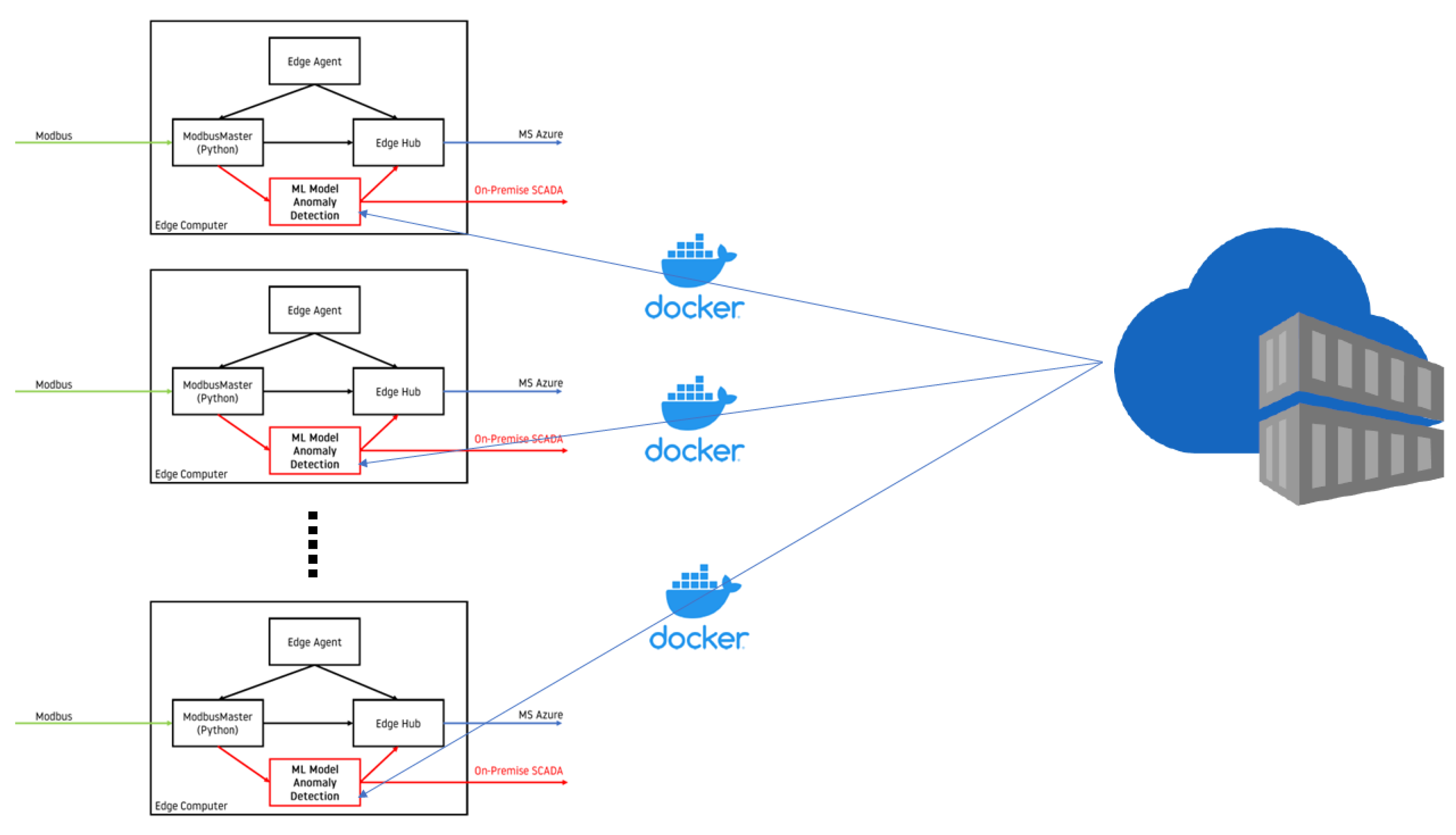
5.1. Make HPU More Independent from Cloud

Using Azure IoTEdge, it is possible to deliver many different kinds of Docker containers on edge devices. The container could contain not just code, there is the possibility to deploy a machine learning model as a *.joblib file within it.
The anomaly detection algorithm described in Section 2.2.3 could be fully deployed as code because it does not contain any black boxes. All that is needed to perform computations are polynomial coefficients and error thresholds. The question is how to provide these values to the edge device. Like the Function App in the cloud, IoTEdge Docker containers on the edge device can have environment variables. Such a mechanism allows us to pass desired parameters to on-premise containers and execute the algorithm flawlessly.
A bit different is the method of deploying the on-premise novelty detection model, the synthesis of which was described in Section 2.2.4. On the grounds that algorithm execution using such a model involves black-box as a scikit-learn *.joblib file. To use this file Docker, the container should be shipped with it. This is possible by performing appropriate actions when building a container.
Deploying algorithms on-premise gives an opportunity to connect to other on-premise components such as SCADA or HMI panels. In such a configuration, HPU operators could be informed on the spot about anomalies without the need to rely on web SCADA. Properly designed algorithms allow diagnostics to be closer to real-time. Expected latency would be related to the period of data taken into consideration. As mentioned in Section 2.3, algorithms so far are designed to be triggered once an hour, so anomalous behavior of HPU could be reported even one hour after the anomaly appears. The time of execution of the Azure Function that performs the calculation is about one second. After one more second, the results computed by Azure Function are visible on MOLOS.CLOUD web SCADA. In total, in the described project, it takes about two seconds from the start of calculations to the presentation of hypotheses when algorithms are embedded in the cloud. When algorithms are embedded on the edge device, the time from the beginning of developing hypotheses using algorithms to the presentation of the results on the on-premise SCADA or HMI panel would be shorter because on-premise calculations would take up less than a second, and the standard on-premise HMI panel refresh rate is less than one second [87].
More frequent analysis in the cloud than assumed so far would result in higher costs of Microsoft Azure Functions service. On-premise, there is no constraint related to monetary cost, so analysis could be performed more frequently and latency could also be reduced according to algorithms triggering frequency.
This way, the edge device can be independent of the cloud computation of analytical hypotheses. However, one crucial aspect should also be mentioned. Applying logic to an edge device implies that the edge device does not have to connect to the internet to detect anomalies. The situation when the range of WiFi or GSM network is unavailable is common when dealing with devices that are working in different places due to their mobility. In turn, the whole solution is more reliable. Access to the internet is important because it could emerge that software inside Docker containers should be updated. However, internet availability all the time is not crucial in this context. The software will be updated if the edge device gets internet connectivity again. Moreover, IoT Edge has the ability to store acquired data on the edge device when the device has no internet access and is able to send the data to the cloud when internet is available again. Data that could be stored is limited due to space on the hard disk on the edge computer. However, in the case of the described project, space on the edge computer is enough to store about a month of measurements. Therefore, the situation when data in the cloud is incomplete is unlikely in the case of mobile HPU which is the subject of the described project.
In conclusion, in the context of making HPU more independent from cloud internet connection is not important for edge devices with IoT Edge when the project is desired to be on-premise. With the use of IoT Edge, on-premise project requirements could be fulfilled because of the ability to store data and compute hypotheses internally. On the other hand, implementing a variant of a project that involves presenting data in the cloud but developing hypotheses on edge devices to make anomaly detection closer to real-time is also possible. In that case, the solution benefits from IoT Edge’s ability to store data internally and send it to the cloud.
A sample architecture of an on-premise IoTEdge solution is presented in Figure 10. Notice that other components of the ecosystem remain untouched. Only an additional Docker container with logic is applied, plus output from Modbus Master is duplicated.
Cost reduction, which is also the profit of making HPU independent from the cloud, is discussed in Section 5.4.

5.2. Algorithms Refinement

In the case of project rollout, many more HPUs will be connected to MOLOS.CLOUD. More devices equals more data. More data equals more reliable hypotheses. For now, reference characteristics were determined based on only one HPU. From a statistical point of view, it is definitely not enough. Nevertheless, industrial practice often does not allow performing innovative projects at scale without proof of concept (PoC).
More data could give fresh insight into data. New dependencies, trends, and features could be extracted. More models could be trained and, as a result, more anomalies could be shown.
Ideally, when new HPUs are plugged in, automatic model retraining should take place. The timer-triggered Azure Function can train models on new data. As a result, new models in the form of *.joblib files and JSON files with polynomial coefficients for each characteristic are uploaded to Azure BLOB storage. There are other methods of iterative model retraining in Azure, but discussion on it is beyond the scope of this article [88].
A summary of the architecture discussed in this paragraph is shown in Figure 11.
Algorithm refinement could also be investigated in the context of used input variables. More variables could be considered as input to anomaly detection algorithms. This includes variables already measured, as well as potential new variables measured from additional sensors. The solution is deployed in production and for that reason, it is not possible to modify algorithms and to change their input variables. However, for future deployments, it is not excluded to expand the solution with additional sensors after detailed consultation with domain experts from PONAR Wadowice. To be coherent with the solution developed so far, potentially new sensors would also be preferably connected to the PLC input module.

5.3. Domain Expertise

Not only could working on raw data deliver profits because of gaining new insights, but consulting hypotheses with domain experts could give some new clues and assumptions.
Furthermore, some kind of active learning [89] could be applied. Circumstances in which detected anomalies and novelties appeared should be carefully analyzed. It would work perfectly if domain experts could give information on whether the detected anomaly was labeled correctly. Such an approach is time-consuming; nevertheless, it could be worth applying in view of the benefits in the future.

5.4. Azure IoTEdge in Deployment at Scale

There is no need to use Docker containers and IoTEdge to fulfill desired project functionalities. It is also possible just to develop pieces of code in Python and run it on an edge device—in this case MOXA UC-8100. Placing data analysis and code inside the Docker container is a bit harder and more time-consuming than developing raw code on the edge device. Especially at the beginning of using such an approach, at a time when Docker and IoTEdge are not well known. However, when it comes to managing more than single-edge devices, it is harder to maintain coherent and stable software and models on all devices.
IoTEdge gives the opportunity to deploy containers at scale. It is possible to order the deployment of the same Docker containers on all edge devices with IoTEdge on board. Receipt for deployment is called deployment manifest [90]. This precisely details which container should be downloaded on devices. Every time some bugfix or feature implementation should be performed, four steps are required to update the software on all edge devices:
  • Perform bugfix, implement feature or refine model/algorithm;
  • Build Docker container;
  • Push container to container repository (ACR or Docker Hub);
  • Deploy it using deployment manifest.
Figure 12 shows schematically the method of deploying and updating containers at scale. Conceptually, it is the same thing as described in Section 5.1. However, this time deployment of containers is made for many devices, not only a single one.
The costs of analytics will scale up approximately linearly while introducing more HPUs into the project. If analytics is placed on-premise, there are no Azure-related costs. Storage for Docker containers (ACR [41] or Docker Hub [40]) is free for purposes and the number of containers provided for the project. Therefore, implementing data analysis on the edge computer is more tempting.

6. Conclusions and Final Thoughts

This article presents a method of combining analytical solutions, edge devices, and SCADA. The subject of the project was a hydraulic power unit (HPU), a high-pressure hydraulic device that fits into the water as a tool concept. Within the project, integration of PLC, edge computer, and Microsoft Azure Cloud was performed. Communication with PLC was performed using the Modbus protocol and communication with Azure IoTHub was established using the MQTT protocol. The code of programs for data acquisition and sending to the cloud was implemented in Python and enclosed within Docker containers with the use of Azure IoTEdge technology. Moreover, developing analytical hypotheses was implemented using Python; however, algorithms that determined whether anomaly occurred or not were executed serverless using Azure Functions and Azure Storage.
Several conclusions could be derived from the work that was carried out in the article. Everything that is presented came from the industrial project and is used in the production of hydraulic power units. The approach to data acquisition, analysis, and presentation could be a reference for other IoT projects. The algorithms described give an insight into what can be important in the context of predictive maintenance and machine monitoring for HPUs. The cost analysis of Azure cloud services and resources used in project implementation was performed, so that the cost of deployment of the project at scale could be more easily estimated.
Innovations that come from the project are algorithms and models designed and developed for a concrete model of HPU. Furthermore, the use of algorithms described in scientific literature distinguishes the project from other commercially implemented solutions. In the literature, there are no presented use cases that involve the IQR statistical measure for hydraulic power units specifically. The use of Microsoft IoTEdge and other components of the Azure Cloud presented in the article was not previously described in the literature in the context of commercial implementation. Furthermore, the method of deploying algorithms, the possibility of rolling out the solution at scale, and the flexibility of the solution to be implemented both in the cloud and on-premise variants are aspects that together are added value that comes from the realization of the described project.
In the current phase of the project, PONAR Wadowice S.A. profits from the ability to monitor and diagnose HPU remotely via web SCADA. Therefore, the goal of the project has been fulfilled. It is important from a business point of view, as a result of the project, that PONAR Wadowice can sell HPU as an innovative product. The business value and effectiveness of the solution are worth inspecting again after gathering more production data.

Author Contributions

Conceptualization, methodology, software, P.F.; writing—original draft preparation, P.F.; writing—review and editing, A.C.; Conceptualization, P.R. All authors have read and agreed to the published version of the manuscript.

Funding

The research is co-financed under the Polish Ministry of Science and Higher Education Program “Doktorat wdrożeniowy”.

Data Availability Statement

Restrictions apply to the availability of these data. Data was obtained from REDNT S.A. and PONAR WADOWICE S.A. and are available from REDNT S.A. and PONAR WADOWICE S.A. with the permission of REDNT S.A. and PONAR WADOWICE S.A.

Acknowledgments

Part of the content of the article was presented on 18 June 2021 at the conference “DSS 2021 ML Edition” (https://ml.dssconf.pl/, accessed on 23 December 2021). Project was implemented in cooperation with PONAR Wadowice S.A. [91] and REDNT S.A. [92].

Conflicts of Interest

The authors declare no conflict of interest.

References

  1. Rednt, S.A. Web-SCADA. Available online: https://molos.cloud/ (accessed on 23 December 2022).
  2. Shevlyakov, G.; Andrea, K.; Choudur, L.; Smirnov, P.; Ulanov, A.; Vassilieva, N. Robust versions of the Tukey boxplot with their application to detection of outliers. In Proceedings of the 2013 IEEE International Conference on Acoustics, Speech and Signal Processing, Vancouver, BC, Canada, 26–31 May 2013; pp. 6506–6510. [Google Scholar] [CrossRef]
  3. Ma, Y.; Hewitt, W.T. Point inversion and projection for NURBS curve and surface: Control polygon approach. Comput. Aided Geom. Des. 2003, 20, 79–99. [Google Scholar] [CrossRef]
  4. Schölkopf, B.; Williamson, R.; Smola, A.; Shawe-Taylor, J.; Platt, J. Support Vector Method for Novelty Detection. In Proceedings of the 12th International Conference on Neural Information Processing Systems, Cambridge, MA, USA, 29 November–4 December 1999; pp. 582–588. [Google Scholar]
  5. Satyro, W.C.; Contador, J.C.; Monken, S.F.D.P.; Lima, A.F.D.; Soares Junior, G.G.; Gomes, J.A.; Neves, J.V.S.; do Nascimento, J.R.; de Araújo, J.L.; Correa, E.D.S.; et al. Industry 4.0 Implementation Projects: The Cleaner Production Strategy—A Literature Review. Sustainability 2023, 15, 2161. [Google Scholar] [CrossRef]
  6. Gomaa, M.; Schade, S.; Bao, D.W.; Xie, Y.M. Automation in rammed earth construction for industry 4.0: Precedent work, current progress and future prospect. J. Clean. Prod. 2023, 398, 136569. [Google Scholar] [CrossRef]
  7. Ryalat, M.; ElMoaqet, H.; AlFaouri, M. Design of a Smart Factory Based on Cyber-Physical Systems and Internet of Things towards Industry 4.0. Appl. Sci. 2023, 13, 2156. [Google Scholar] [CrossRef]
  8. Wang, M.; Xu, C.; Lin, Y.; Lu, Z.; Sun, J.; Gui, G. A Distributed Sensor System Based on Cloud-Edge-End Network for Industrial Internet of Things. Future Internet 2023, 15, 171. [Google Scholar] [CrossRef]
  9. Thayyib, P.V.; Mamilla, R.; Khan, M.; Fatima, H.; Asim, M.; Anwar, I.; Shamsudheen, M.K.; Khan, M.A. State-of-the-Art of Artificial Intelligence and Big Data Analytics Reviews in Five Different Domains: A Bibliometric Summary. Sustainability 2023, 15, 4026. [Google Scholar] [CrossRef]
  10. Alghamdi, A.S.; Rahman, A. Data Mining Approach to Predict Success of Secondary School Students: A Saudi Arabian Case Study. Educ. Sci. 2023, 13, 293. [Google Scholar] [CrossRef]
  11. Jedrzykiewicz, Z.; Stojek, J.; Rosikowski, P. Naped i Sterowanie Hydrostatyczne, Monograph; Vist Sp. z o.o.: Dąbrowa Górnicza, Poland, 2017; p. 557. [Google Scholar]
  12. Chatterjee, A.; Ahmed, B.S. IoT anomaly detection methods and applications: A survey. Internet Things 2022, 19, 100568. [Google Scholar] [CrossRef]
  13. Belichovski, M.; Stavrov, D.; Donchevski, F.; Nadzinski, G. Unsupervised Machine Learning Approach for Anomaly Detection in E-coating Plant. In Proceedings of the 2022 IEEE 17th International Conference on Control &Automation (ICCA), Naples, Italy, 27–30 June 2022; pp. 992–997. [Google Scholar] [CrossRef]
  14. Samara, M.A.; Bennis, I.; Abouaissa, A.; Lorenz, P. A Survey of Outlier Detection Techniques in IoT: Review and Classification. J. Sens. Actuator Netw. 2022, 11, 4. [Google Scholar] [CrossRef]
  15. Wan, X.; Farmani, R.; Keedwell, E. Online leakage detection system based on EWMA-enhanced Tukey method for water distribution systems. J. Hydroinform. 2022, 25, 51–69. [Google Scholar] [CrossRef]
  16. Beghi, A.; Cecchinato, L.; Corazzol, C.; Rampazzo, M.; Simmini, F.; Susto, G. A One-Class SVM Based Tool for Machine Learning Novelty Detection in HVAC Chiller Systems. IFAC Proc. Vol. 2014, 47, 1953–1958. [Google Scholar] [CrossRef] [Green Version]
  17. Keleko, A.T.; Kamsu-Foguem, B.; Ngouna, R.H.; Tongne, A. Health condition monitoring of a complex hydraulic system using Deep Neural Network and DeepSHAP explainable XAI. Adv. Eng. Softw. 2023, 175, 103339. [Google Scholar] [CrossRef]
  18. Wu, Z.Y.; Chew, A.; Meng, X.; Cai, J.; Pok, J.; Kalfarisi, R.; Lai, K.C.; Hew, S.F.; Wong, J.J. High Fidelity Digital Twin-Based Anomaly Detection and Localization for Smart Water Grid Operation Management. Sustain. Cities Soc. 2023, 91, 104446. [Google Scholar] [CrossRef]
  19. Tziolas, T.; Papageorgiou, K.; Theodosiou, T.; Papageorgiou, E.; Mastos, T.; Papadopoulos, A. Autoencoders for Anomaly Detection in an Industrial Multivariate Time Series Dataset. Eng. Proc. 2022, 18, 23. [Google Scholar] [CrossRef]
  20. Zhou, B.; Pychynski, T.; Reischl, M.; Kharlamov, E.; Mikut, R. Machine learning with domain knowledge for predictive quality monitoring in resistance spot welding. J. Intell. Manuf. 2022, 33, 1139–1163. [Google Scholar] [CrossRef]
  21. Voigt, T.; Kohlhase, M.; Nelles, O. Incremental DoE and Modeling Methodology with Gaussian Process Regression: An Industrially Applicable Approach to Incorporate Expert Knowledge. Mathematics 2021, 9, 2479. [Google Scholar] [CrossRef]
  22. Coelho, D.; Costa, D.; Rocha, E.M.; Almeida, D.; Santos, J.P. Predictive maintenance on sensorized stamping presses by time series segmentation, anomaly detection, and classification algorithms. Procedia Comput. Sci. 2022, 200, 1184–1193. [Google Scholar] [CrossRef]
  23. Kim, D.; Heo, T.Y. Anomaly Detection with Feature Extraction Based on Machine Learning Using Hydraulic System IoT Sensor Data. Sensors 2022, 22, 2479. [Google Scholar] [CrossRef]
  24. Maggipinto, M.; Beghi, A.; Susto, G.A. A Deep Convolutional Autoencoder-Based Approach for Anomaly Detection with Industrial, Non-Images, 2-Dimensional Data: A Semiconductor Manufacturing Case Study. IEEE Trans. Autom. Sci. Eng. 2022, 19, 1477–1490. [Google Scholar] [CrossRef]
  25. Chohra, A.; Shirani, P.; Karbab, E.B.; Debbabi, M. Chameleon: Optimized feature selection using particle swarm optimization and ensemble methods for network anomaly detection. Comput. Secur. 2022, 117, 102684. [Google Scholar] [CrossRef]
  26. Gong, X.; Yu, L.; Wang, J.; Zhang, K.; Bai, X.; Pal, N.R. Unsupervised feature selection via adaptive autoencoder with redundancy control. Neural Netw. 2022, 150, 87–101. [Google Scholar] [CrossRef]
  27. Ali, O.; Ishak, M.K.; Bhatti, M.K.L.; Khan, I.; Kim, K.I. A Comprehensive Review of Internet of Things: Technology Stack, Middlewares, and Fog/Edge Computing Interface. Sensors 2022, 22, 995. [Google Scholar] [CrossRef] [PubMed]
  28. Kumar, A.; Saha, R.; Alazab, M.; Kumar, G. A Lightweight Signcryption Method for Perception Layer in Internet-of-Things. J. Inf. Secur. Appl. 2020, 55, 102662. [Google Scholar] [CrossRef]
  29. SIMATIC S7-400 Documentation. Available online: https://new.siemens.com/global/en/products/automation/systems/industrial/plc/simatic-s7-400.html (accessed on 13 May 2023).
  30. SIEMENS S7 Comparison. Available online: https://cache.industry.siemens.com/dl/files/648/109797648/att_1067421/v1/s71500_compare_table_en.pdf (accessed on 14 May 2023).
  31. SIEMENS MindSphere. Available online: https://www.plm.automation.siemens.com/global/pl/products/mindsphere/ (accessed on 14 May 2023).
  32. MOXA Industrial Linux. Available online: https://www.moxa.com/en/products/industrial-computing/system-software/moxa-industrial-linux (accessed on 11 May 2022).
  33. Python Package for Modbus Handling. Version: 2.5.3. Available online: https://pymodbus.readthedocs.io/en/latest/index.html (accessed on 4 December 2022).
  34. Azure IoT-SDK-Python. Available online: https://github.com/Azure/azure-iot-sdk-python (accessed on 16 March 2022).
  35. Docker-Based Ecosystem for Deploying Software on Edge Devices. Available online: https://azure.microsoft.com/en-us/services/iot-edge/ (accessed on 4 December 2022).
  36. Docker Official Website. Available online: https://docker.com/ (accessed on 22 December 2022).
  37. Azure-CLI. Available online: https://docs.microsoft.com/en-us/cli/azure/ (accessed on 22 December 2022).
  38. Portal Azure. Available online: https://portal.azure.com/ (accessed on 22 December 2022).
  39. Docker CLI. Available online: https://docs.docker.com/engine/reference/commandline/cli/ (accessed on 16 December 2022).
  40. Docker Hub. Available online: https://hub.docker.com/_/registry (accessed on 22 December 2022).
  41. Azure Container Registry. Available online: https://azure.microsoft.com/en-us/services/container-registry/ (accessed on 22 December 2022).
  42. Basseville, M.; Nikiforov, I.V. Detection of abrupt changes: Theory and application. Technometrics 1993, 36, 550. [Google Scholar]
  43. Deshcherevskii, A.V.; Sidorin, A.Y. Iterative algorithm for time series decomposition into trend and seasonality: Testing using the example of CO2 concentrations in the atmosphere. Izv. Atmos. Ocean. Phys. 2021, 57, 813–836. [Google Scholar] [CrossRef]
  44. Talagala, P.; Hyndman, R.; Smith-Miles, K.; Kandanaarachchi, S.; Muñoz, M. Anomaly detection in streaming nonstationary temporal data. J. Comput. Graph. Stat. 2020, 29, 13–27. [Google Scholar] [CrossRef]
  45. Schmidl, S.; Wenig, P.; Papenbrock, T. Anomaly Detection in Time Series: A Comprehensive Evaluation. Proc. VLDB Endow. PVLDB 2022, 15, 1779–1797. [Google Scholar] [CrossRef]
  46. Akoglu, H. User’s guide to correlation coefficients. Turk. J. Emerg. Med. 2018, 18, 91–93. [Google Scholar] [CrossRef]
  47. Harris, C.R.; Millman, K.J.; van der Walt, S.J.; Gommers, R.; Virtanen, P.; Cournapeau, D.; Wieser, E.; Taylor, J.; Berg, S.; Smith, N.J.; et al. Array programming with NumPy. Nature 2020, 585, 357–362. [Google Scholar] [CrossRef]
  48. Linear Regression Explanation. Available online: http://www.stat.yale.edu/Courses/1997-98/101/linreg.htm (accessed on 16 March 2022).
  49. Torabi, H.; Mirtaheri, S.L.; Greco, S. Practical autoencoder based anomaly detection by using vector reconstruction error. Cybersecurity 2023, 6, 1. [Google Scholar] [CrossRef]
  50. Hosseinzadeh, M.; Rahmani, A.M.; Vo, B.; Bidaki, M.; Masdari, M.; Zangakani, M. Improving security using SVM-based anomaly detection: Issues and challenges. Soft Comput. 2021, 25, 3195–3223. [Google Scholar] [CrossRef]
  51. Miljkovic, D. Review of novelty detection methods. In Proceedings of the 33rd International Convention MIPRO, Opatija, Croatia, 24–28 May 2010; pp. 593–598. [Google Scholar]
  52. One Class SVM in Scikit-Learn Python Package. Available online: https://scikit-learn.org/stable/modules/generated/sklearn.svm.OneClassSVM.html (accessed on 16 April 2022).
  53. Huang, G.; Chen, J.; Liu, L. One-Class SVM Model-Based Tunnel Personnel Safety Detection Technology. Appl. Sci. 2023, 13, 1734. [Google Scholar] [CrossRef]
  54. Chen, L.; Buhong, W.; Jiwei, T.; Rongxiao, G. Anomaly detection method for UAV sensor data based on LSTM-OCSVM. J. Chin. Comput. Syst. 2021, 42, 700–705. [Google Scholar]
  55. Peng, T.; Li, C.; Zhou, X. Application of machine learning to laboratory safety management assessment. Saf. Sci. 2019, 120, 263–267. [Google Scholar] [CrossRef]
  56. Azure Functions Description. Available online: https://azure.microsoft.com/en-us/services/functions/ (accessed on 22 December 2022).
  57. Hassan, H.B.; Barakat, S.A.; Sarhan, Q.I. Survey on serverless computing. J. Cloud Comput. Adv. Syst. Appl. 2021, 10, 39. [Google Scholar] [CrossRef]
  58. Ways of Triggering Azure Functions. Available online: https://docs.microsoft.com/en-us/learn/modules/execute-azure-function-with-triggers/ (accessed on 22 December 2022).
  59. Exporting and Importing Model as *.joblib File. Available online: https://scikit-learn.org/stable/model_persistence.html (accessed on 12 April 2022).
  60. Documentation of ModbusSlave Software. Version: 9. Available online: https://www.modbustools.com/modbus_slave.html (accessed on 15 March 2023).
  61. Description of Azure Function App as Consumpion Plan. Available online: https://docs.microsoft.com/en-us/azure/azure-functions/consumption-planl (accessed on 22 December 2022).
  62. Available online: https://learn.microsoft.com/en-us/azure/network-watcher/traffic-analytics (accessed on 15 May 2023).
  63. Available online: https://stackoverflow.com/questions/70501366/azure-pricing-calculator-for-hours-in-cloud-service (accessed on 15 May 2023).
  64. Azure-Stream-Analytics. Available online: https://azure.microsoft.com/en-us/services/stream-analytics/ (accessed on 16 December 2022).
  65. Available online: https://www.microsoft.com/en-us/download/details.aspx?id=56519 (accessed on 15 May 2023).
  66. Available online: https://learn.microsoft.com/en-us/azure/iot-hub/iot-hub-mqtt-support (accessed on 15 May 2023).
  67. Goodfellow, I.; Bengio, Y.; Courville, A. Deep Learning; MIT Press: Cambridge, MA, USA, 2016; p. 117. Available online: http://www.deeplearningbook.org (accessed on 29 December 2022).
  68. Sun, C.; He, Z.; Lin, H.; Cai, L.; Cai, H.; Gao, M. Anomaly detection of power battery pack using gated recurrent units based variational autoencoder. Appl. Soft Comput. 2023, 132, 109903. [Google Scholar] [CrossRef]
  69. Saha, S.; Sarkar, J.; Dhavala, S.; Sarkar, S.; Mota, P. Quantile LSTM: A Robust LSTM for Anomaly Detection In Time Series Data. arXiv 2023, arXiv:2302.08712. [Google Scholar]
  70. Park, M.H.; Chakraborty, S.; Vuong, Q.D.; Noh, D.H.; Lee, J.W.; Lee, J.U.; Choi, J.H.; Lee, W.J. Anomaly Detection Based on Time Series Data of Hydraulic Accumulator. Sensors 2022, 22, 9428. [Google Scholar] [CrossRef]
  71. Kang, H.S.; Choi, Y.S.; Yu, J.S.; Jin, S.W.; Lee, J.M.; Kim, Y.J. Hyperparameter Tuning of OC-SVM for Industrial Gas Turbine Anomaly Detection. Energies 2022, 15, 8757. [Google Scholar] [CrossRef]
  72. Guan, S.; Zhao, B.; Dong, Z.; Gao, M.; He, Z. GTAD: Graph and Temporal Neural Network for Multivariate Time Series Anomaly Detection. Entropy 2022, 24, 759. [Google Scholar] [CrossRef]
  73. Perez-Padillo, J.; García Morillo, J.; Ramirez-Faz, J.; Torres Roldán, M.; Montesinos, P. Design and Implementation of a Pressure Monitoring System Based on IoT for Water Supply Networks. Sensors 2020, 20, 4247. [Google Scholar] [CrossRef]
  74. Anton, A.A.; Cococeanu, A.; Muntean, S. Software for Monitoring the In-Service Efficiency of Hydraulic Pumps. Appl. Sci. 2022, 12, 11450. [Google Scholar] [CrossRef]
  75. Robyns, S.; Helsen, S.; Weckx, S.; Bhoi, S.K.; Baghdadi, M.E.; Hegazy, O.; De Smet, J. An intelligent data capturing framework to improve condition monitoring and anomaly detection for industrial machines. Procedia Comput. Sci. 2023, 217, 709–719. [Google Scholar] [CrossRef]
  76. Derse, C.; El Baghdadi, M.; Hegazy, O.; Sensoz, U.; Gezer, H.N.; Nil, M. An Anomaly Detection Study on Automotive Sensor Data Time Series for Vehicle Applications. In Proceedings of the 2021 Sixteenth International Conference on Ecological Vehicles and Renewable Energies (EVER), Monte-Carlo, Monaco, 5–7 May 2021; pp. 1–5. [Google Scholar] [CrossRef]
  77. Motulsky, H.J.; Brown, R.E. Detecting outliers when fitting data with nonlinear regression—A new method based on robust nonlinear regression and the false discovery rate. BMC Bioinform. 2006, 7, 123. [Google Scholar] [CrossRef] [Green Version]
  78. Pang, J.; Pu, X.; Li, C. A Hybrid Algorithm Incorporating Vector Quantization and One-Class Support Vector Machine for Industrial Anomaly Detection. IEEE Trans. Ind. Inform. 2022, 18, 8786–8796. [Google Scholar] [CrossRef]
  79. Arunthavanathan, R.; Khan, F.; Ahmed, S.; Imtiaz, S. Autonomous Fault Diagnosis and Root Cause Analysis for the Processing System Using One-Class SVM and NN Permutation Algorithm. Ind. Eng. Chem. Res. 2022, 61, 1408–1422. [Google Scholar] [CrossRef]
  80. Li, X.; Xu, Y.; Li, N.; Yang, B.; Lei, Y. Remaining Useful Life Prediction With Partial Sensor Malfunctions Using Deep Adversarial Networks. IEEE/CAA J. Autom. Sin. 2023, 10, 121–134. [Google Scholar] [CrossRef]
  81. Li, D.; Zhou, Y.; Hu, G.; Spanos, C.J. Handling Incomplete Sensor Measurements in Fault Detection and Diagnosis for Building HVAC Systems. IEEE Trans. Autom. Sci. Eng. 2020, 17, 833–846. [Google Scholar] [CrossRef]
  82. Perales Gómez, Á.L.; Maimó, L.F.; Celdrán, A.H.; Clemente, F.J.G. SUSAN: A Deep Learning based anomaly detection framework for sustainable industry. Sustain. Comput. Inform. Syst. 2023, 37, 100842. [Google Scholar] [CrossRef]
  83. Peco Chacón, A.M.; Segovia Ramirez, I.; García Márquez, F.P. False alarm detection in wind turbine by classification models. Adv. Eng. Softw. 2023, 177, 103409. [Google Scholar] [CrossRef]
  84. ELMARK MOXA. Available online: https://www.elmark.com.pl/sklep/moxa/uc-8100-me-t (accessed on 14 May 2023).
  85. TIBCO. Available online: https://community.tibco.com/s/article/anomaly-detection-and-root-cause-analysis-using-tibco-analytics-and-microsoft-cognitive (accessed on 14 May 2023).
  86. Crosser. Available online: https://crosser.io/resources/webinars-and-videos/webinars/iot/anomaly-detection-with-crossers-low-code-platform/?gclid=CjwKCAjwjYKjBhB5EiwAiFdSfircXqSPDMpjlZqzmzRIQ5DWH3if7I1KbGS236n9Bmf2jmSHuLuffxoCuwYQAvD_BwE (accessed on 14 May 2023).
  87. Bowen, C.L.; Buennemeyer, T.; Thomas, R. Next generation SCADA security: Best practices and client puzzles. In Proceedings of the Sixth Annual IEEE SMC Information Assurance Workshop, West Point, NY, USA, 15–17 June 2005; pp. 426–427. [Google Scholar]
  88. Available online: https://docs.microsoft.com/en-us/azure/machine-learning/\v1/how-to-deploy-azure-container-instance (accessed on 22 December 2022).
  89. Holzinger, A. Interactive machine learning for health informatics: When do we need the human-in-the-loop? Brain Inform. 2016, 3, 119–131. [Google Scholar] [CrossRef] [PubMed] [Green Version]
  90. Way of Deploying IoTEdge Containers at Scale. Available online: https://docs.microsoft.com/en-us/azure/iot-edge/module-deployment-monitoring?view=iotedge-2020-11 (accessed on 11 May 2022).
  91. PONAR Wadowice S.A. Webpage. Available online: https://www.ponar-wadowice.pl/ (accessed on 4 December 2022).
  92. REDNT S.A. Webpage. Available online: https://rednt.eu (accessed on 21 December 2022).
Figure 1. Photo of the hydraulic power unit that is the subject of the project.
Futureinternet 15 00206 g001
Figure 2. Communication scheme.
Futureinternet 15 00206 g002
Figure 3. IoTEdge ecosystem deployed on edge device.
Futureinternet 15 00206 g003
Figure 4. Correlation matrix with several most correlated variables.
Futureinternet 15 00206 g004
Figure 5. Scatter plot with fitted curve—power due to fuel consumption.
Futureinternet 15 00206 g005
Figure 6. Scatter plot with fitted curve—pressure due to rotation.
Futureinternet 15 00206 g006
Figure 7. Cloud ecosystem for deploying algorithms into production.
Futureinternet 15 00206 g007
Figure 8. Deviations power vs. fuel.
Futureinternet 15 00206 g008
Figure 9. Deviations pressure vs. rotation.
Futureinternet 15 00206 g009
Figure 10. IoTEdge ecosystem enriched in ML model deployed as Docker container.
Futureinternet 15 00206 g010
Figure 11. Refinement pipeline for algorithms proposal.
Futureinternet 15 00206 g011
Figure 12. IoTEdge ecosystem enriched in ML model deployed as Docker container at scale.
Futureinternet 15 00206 g012
Table 1. Values of quadratic function coefficients for fitted curves rounded to two significant digits.
Characteristicsabc
Power mean vs. fuel consumption mean 1.5 × 10 ( 4 ) 3.3 × 10 ( 1 ) −4.1
Pressure behind filter vs. rotation speed mean1.8 6.3 × 10 ( 4 ) 1.5 × 10 ( 1 )
Table 2. Error thresholds calculated using IQR Criterion.
CharacteristicsError Threshold
Power mean vs. fuel consumption mean10.4
Pressure behind filter vs. rotation speed mean0.998
Disclaimer/Publisher’s Note: The statements, opinions and data contained in all publications are solely those of the individual author(s) and contributor(s) and not of MDPI and/or the editor(s). MDPI and/or the editor(s) disclaim responsibility for any injury to people or property resulting from any ideas, methods, instructions or products referred to in the content.

