Synchronizing Many Filesystems in Near Linear Time

Abstract

Finding a provably correct subquadratic synchronization algorithm for many filesystem replicas is one of the main theoretical problems in operational transformation (OT) and conflict-free replicated data types (CRDT) frameworks. Based on the algebraic theory of filesystems, which incorporates non-commutative filesystem commands natively, we developed and built a proof-of-concept implementation of an algorithm suite which synchronizes an arbitrary number of replicas. The result is provably correct, and the synchronized system is created in linear space and time after an initial sorting phase. It works by identifying conflicting command pairs and requesting one of the commands to be removed. The method can be guided to reach any of the theoretically possible synchronized states. The algorithm also allows asynchronous usage. After the client sends a synchronization request, the local replica remains available for further modifications. When the synchronization instructions arrive, they can be merged with the changes made since the synchronization request. The suite also works on filesystems with a directed acyclic graph-based path structure in place of the traditional tree-like arrangement. Consequently, our algorithms apply to filesystems with hard or soft links as long as the links create no loops.

1. Introduction and Related Works

Synchronizing diverged copies of some data stored on a variety of devices and/or at different locations is an ubiquitous task. The last two decades saw a proliferation of practical and theoretical works addressing this problem. According to [1], “file synchronization is a feature usually included with backup software in order to make is easier to manage and recover data as and when required”. File synchronization is usually delivered through cloud services. Dedicated file synchronizing solutions frequently come with additional tools not just for managing the saved data but also to allow for file sharing and collaboration with stored files and documents.

These cloud storage services are easily accessible for the end user because the service front ends are very well integrated into web clients as well as desktop and mobile environments. Simple user interfaces hide the complex and sophisticated service back ends [2]. Collaboration services are frequently integrated into the “cloud storage” environment. For example, Google Docs is an application layer integrated into Google Drive storage, Office 365 is integrated with One Drive storage and Dropbox Paper service is an extension of Dropbox storage.

To address the emerging challenges in the more specific fields of distributed data storage and collaborative editors, two competing theoretical frameworks emerged: operational transformation (OT) and conflict-free (or commutative) replicated data types (CRDT). OT appeared in the seminal work of [3] and was refined later, among others, in [4,5,6]. The main applications are collaborative editors, the most notable example being Google Docs [7]. CRDT emerged as an alternative with a stronger theoretical background, see [8,9]. Both OT and CRDT have been applied successfully in a variety of synchronization tasks, including file synchronizers [6,10,11]. Finding a provably correct, subquadratic synchronization algorithm, however, has remained one of the main open problems both in OT and CRDT [12].

The algebraic theory of filesystems [13,14] introduced algebraic manipulations of filesystem commands, and provided the foundations for automated checking of certain filesystem properties. It is reminiscent of both OT [6] and CRDT inasmuch as, instead of pure traditional filesystem commands, it uses operations enriched with contextual information. While these operations are not fully commutative—as would be requested by CRDT [15]—the non-commutative parts can be isolated systematically and handled separately. In [14], this framework is used successfully to create a provably correct theoretical filesystem synchronizer for two replicas together with a complete analysis of all possible synchronized states. The present work extends [14] significantly by the following:

–

Providing the theoretical foundation for synchronizing an arbitrary number of replicas;

–

Developing, for the first time, a provably correct synchronization algorithm which works in linear time after an initial sort, and thus in subquadratic total running time;

–

Allowing asynchronous usage, namely, after requesting synchronization, the local replicas need not be locked;

–

Allowing for late comers when a replica can be upgraded to the synchronized state without providing the local changes;

–

Generalizing the traditional tree-like filesystem skeleton to arbitrary acyclic graphs, thus extending the applicability of the synchronization algorithm.

In this paper, we will use the term near linear to mean “linear up to a logarithmic factor”. Thus, sorting requires near linear time [16], and the total time required by the above synchronization algorithm is also near linear.

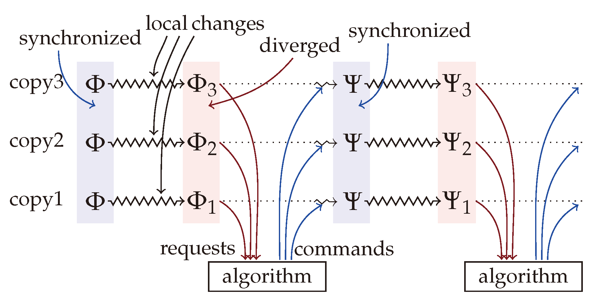
This paper follows the traditional paradigm of filesystem synchronization described in, for example, [17] and illustrated in Figure 1. The starting point is a set of identical copies of the same filesystem, possibly stored at different locations, on different hardware and architectures (cloud servers, mobile devices, laptop and desktop computers with various operating systems) or using different software implementations (e.g., ext4, btrfs, ZFS, NTFS, APFS, or database file systems). Each of these replicas is edited (modified) locally. At a certain time, the diverged copies call for synchronization by sending a description of the diverged state to a central server. After receiving the requests, the server computes filesystem commands, which transform each replica into a common synchronized state, and send them back to the replicas. The replicas execute the received commands on their local copy, transforming all diverged copies into a new identical synchronized state. At that point, the synchronization cycle can start again.

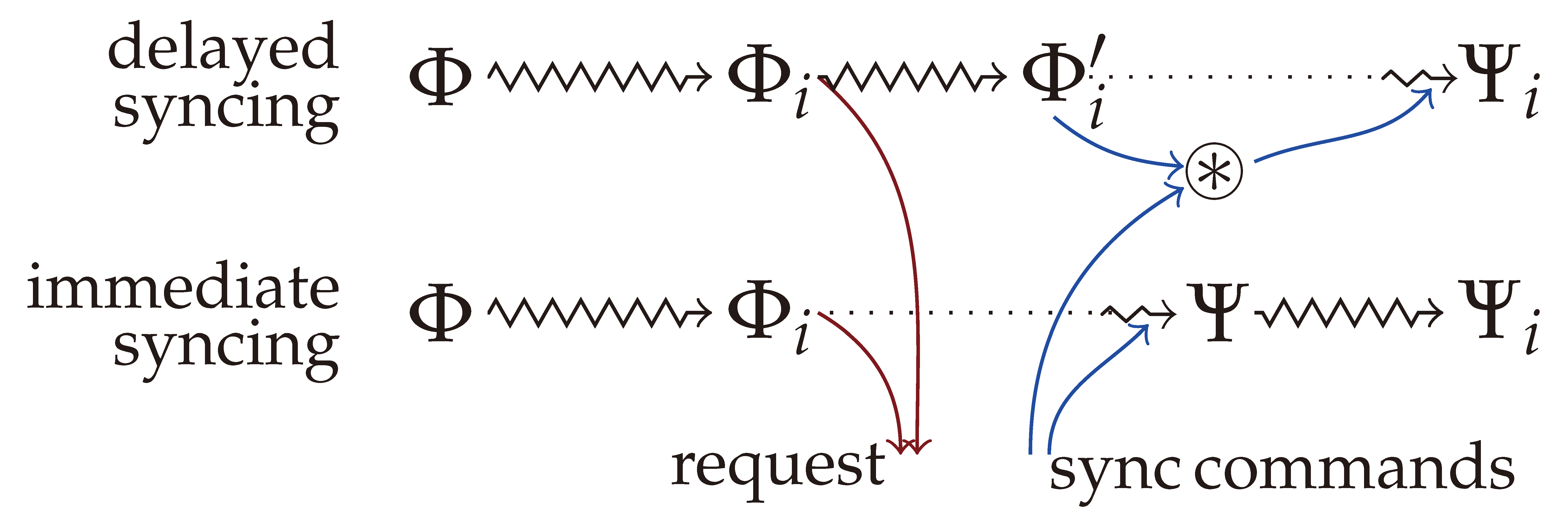
Synchronizers typically require locking the replicas during the whole synchronization process, meaning that no modifications are allowed after the synchronization request is sent (the locked time period is indicated by the dotted lines on Figure 1). Asynchronous, or optimistic synchronization allows additional local modifications after the synchronization request is sent as depicted on the top of Figure 2. When the synchronization commands arrive from the server, those commands are modified to reflect the additional changes, and then applied to the replica. The result should be the same as when performing synchronization without the additional changes, and then applying them to the synchronized filesystem afterwards—as indicated at the bottom of the figure.

The main focus of this paper is filesystem synchronization, or the synchronization of data stored in the nodes of a tree or directed acyclic graph. The stored data are considered to be an indivisible unit, and the task of consolidating different versions of the same data is not considered. It should be solved by other methods specifically tailored to this task.

Some practical aspects of data synchronization are not touched and are out of the scope of this paper. Managing user access and permissions, when and how to allow file sharing and collaboration are especially important due to security considerations [1]. Additionally, file synchronization should use very strict security protocols to ensure that data are safely protected and secured at all times and to make data leaks and malicious access less likely.

Synchronizers should also minimize network traffic. Unlike the popular Rsync utility [18] available for comparing and synchronizing files, there is currently no such “middleware” utility for general datasets [19]. Hopefully our work is a small step in that direction.

The rest of this paper is organized as follows. Section 2 recalls the building blocks of the algebraic theory of filesystems, including the filesystem model, the augmented filesystem commands and their basic properties. This section does not contain new results, and its purpose is to give the reader a comprehensive summary of the topic, on which the rest of the paper relies. For more intuition, explanation and examples, please consult [14]. Section 3 is a high-level overview of how filesystem synchronization can be handled in the algebraic framework. This section defines what constitutes a synchronized state of several diverged replicas, rather than providing a method of creating it. The definition automatically guarantees many desired and required properties of the merged filesystem, an indication of the strength and adequacy of the algebraic framework. It is discussed how all synchronized states can be achieved by conflict resolution, paving the way towards the near linear synchronization algorithm discussed in Section 4 and Section 6. Asynchronous (optimistic) synchronization is discussed at the end of Section 3.

The base algorithms of the synchronization suite are discussed in Section 4, including the one which generates the command sequence (called merger), which produces the merged state in subquadratic time. Supporting theoretical results are collected and proved in Section 5. Section 6 discusses how all possible synchronized states can be generated by a nondeterministic algorithm running in linear time. Section 7 presents some empirical results justifying the claims about the running time of the algorithms. Finally, Section 8 concludes the paper with some extensions and open problems. Most notably, our algorithms, with some modification, work not only on the tree-like filesystem skeletons as stipulated by the algebraic theory but also on filesystems based on directed acyclic graphs.

This work focuses mainly on algorithmic aspects, so many theoretical justifications are deliberately phrased in general terms. Rigorous proofs would require substantially more space and, in our opinion, would not provide additional insight. A proof-of-concept implementation of the algorithms presented in this paper in Python can be found at https://github.com/csirmaz/algebraic-reconciler (accessed on 10 May 2023).

2. Definitions

This section recalls the notions and basic results of the algebraic theory of filesystems [13], with some illustration of the concepts. The main component is a highly symmetric set of filesystem commands, which are enriched with contextual information. Devising such a command set which is amenable to algebraic manipulation was one of the main contributions of [13]. For more intuition and explanation on this, see [14].

2.1. Filesystems

The filesystem model reflects the most important high-level aspects of real-world filesystems. It is a mixture of identity- and path-based models [10,12]. The contents of the filesystem are stored at nodes, which are identified, or labeled, by a set of fixed and predetermined paths. The collection of all (virtually) available nodes is fixed in advance (while in a real-world filesystem, only a restricted subset of those paths is present). No path operations are considered; in particular, our model does not support the creation or deletion of links. In the basic case, no links are allowed at all; thus, the namespace—the set of available nodes or paths—forms a collection of rooted trees. An actual filesystem populates this fixed namespace with values. If $\mathsf{\Phi }$ is a filesystem, the value stored at node n is denoted by $\mathsf{\Phi }\left(n\right)$. Valid filesystems are required to have the tree property all the time, meaning that along any branch starting from a root node, there must be zero or more directories, zero or one file, followed by empty nodes only. If $\mathsf{\Phi }$ does not have the tree property, then we say that $\mathsf{\Phi }$ is broken.

Formally, the paths form a forest-like namespace: a set $\mathbb{N}$ endowed with the partial function $\uparrow :\mathbb{N}\to \mathbb{N}$ returning the parent of every non-root node, while this function is not defined on roots. If $n=\uparrow m$ then n is the parent of m, and m is a child of n. For two nodes $n,m\in \mathbb{N}$, we say that n is above m, or n is an ancestor of m, and write $n\prec m$, if $n={\uparrow }^{i}m$ for some $i\ge 1$. As usual, $n\preccurlyeq m$ denotes $n\prec m$ or $n=m$. As the parent function ↑ induces a tree-like structure on $\mathbb{N}$, the relation ≼ is a partial order. Two nodes $n,m\in \mathbb{N}$ are comparable if either $n\preccurlyeq m$ or $m\preccurlyeq n$, and they are incomparable or independent otherwise.

In practice, nodes of the filesystem are labeled by complete paths, where directory names are separated by the slash character. Thus, the root has the label $/$; nodes $/\mathsf{a}$, $/\mathsf{x}\mathsf{x}\mathsf{x}$ are on the first level just under the root; and $/\mathsf{a}/\mathsf{b}/\mathsf{c}\mathsf{c}/\mathsf{d}$ is (the label of) a node on level four, whose ancestors are $/\mathsf{a}/\mathsf{b}/\mathsf{c}\mathsf{c}$, $/\mathsf{a}/\mathsf{b}$, $/\mathsf{a}$, and $/$. The implementation of the algorithms also follows this convention.

As indicated above, the value stored by a filesystem at a node can be a directory, can be empty or can be a file. The type of this value is denoted by $\mathbb{D}$, $\mathbb{O}$ and $\mathbb{F}$, respectively, corresponding to these possibilities. Regarding notation, we also use $\mathbb{D}$ for the directory value, and $\mathbb{O}$ for the empty value (where $\mathbb{O}$ means “no value”, not to be confused with a file which has no content). When the node value is a file, then the node stores the complete file content (including the possibility that this content is empty). While this filesystem model allows only one directory value and only one empty value (see the discussion in Section 8 on relaxing this limitation), there are many different possible file values of type $\mathbb{F}$ representing different file contents. The value types are ordered, with $\mathbb{O}$ being the lowest, and $\mathbb{D}$ being the highest, written as $\mathbb{O}<\mathbb{F}<\mathbb{D}$. The type of the filesystem value x is denoted by $\mathrm{tp}\left(x\right)$.

2.2. Filesystem Commands

Real-life filesystems are usually manipulated by commands such as creating or deleting files and directories, modifying (editing, appending to) a file, or moving an existing file or directory to another location. Our model contains similar commands but with some modifications, the first of which is that we only consider commands which affect the filesystem at a single node. Thus, a move command should be represented as a sequence of delete and create.

Second, commands in our model include the complete new value to be stored in the filesystem. Even if file contents are just partially modified or are appended to, the full new value must be supplied. This allows our model to use a unified representation of all single-node commands, as they can be fully specified by the node (path), at which the command acts, and the new value (including a directory and empty value) to be stored there.

Third, as was observed in [13], enriching filesystem commands with additional contextual information—in this case, the previous content at the affected node—makes them amenable to algebraic manipulation.

Definition 1 

(Filesystem commands). A filesystem command is a triplet $\sigma =\langle n,x,y\rangle$, where $n\in \mathbb{N}$ is the node on which σ acts, x is the content at node n before σ is executed (the contextual information, precondition), and y is the new content.

It is clear that every real-life filesystem command acting on a single node can be easily (and automatically) transformed into this internal representation (Definition 1). For example, rmdir$\left(n\right)$ corresponds to $\langle n,\mathbb{D},\mathbb{O}\rangle$, which replaces the directory value at n by the empty value. The command $\langle n,\mathbb{O},\mathbb{D}\rangle$ creates a directory at n but only if the node n has no content, that is, there is no directory or file at n (a usual requirement when creating a directory). This command reflects the usual behavior or mkdir. For files f₁ and f₂ $\in \mathbb{F}$, the command $\langle n,{\mathsf{f}}_1,{\mathsf{f}}_2\rangle$ replaces 1 stored at n by the new content f₂. This latter command can be considered an equivalent of edit$(n,{\mathsf{f}}_2)$.

As an example, creating a copy of the file $/\mathsf{h}\mathsf{o}\mathsf{m}\mathsf{e}/\mathsf{u}\mathsf{s}\mathsf{e}\mathsf{r}/\mathsf{t}\mathsf{e}\mathsf{x}\mathsf{t}$ in the same directory under the name “$\mathsf{c}\mathsf{o}\mathsf{p}\mathsf{y}$” and then deleting the original file is represented by the following sequence of commands:

$$\langle /\mathsf{h}\mathsf{o}\mathsf{m}\mathsf{e}/\mathsf{u}\mathsf{s}\mathsf{e}\mathsf{r}/\mathsf{c}\mathsf{o}\mathsf{p}\mathsf{y},\mathbb{O},{\mathsf{f}}_o\rangle \mathrm{and}\langle /\mathsf{h}\mathsf{o}\mathsf{m}\mathsf{e}/\mathsf{u}\mathsf{s}\mathsf{e}\mathsf{r}/\mathsf{t}\mathsf{e}\mathsf{x}\mathsf{t},{\mathsf{f}}_o,\mathbb{O}\rangle ,$$

where f_o is the file content at the “$\mathsf{t}\mathsf{e}\mathsf{x}\mathsf{t}$” node.

Applying the command $\sigma$ to a filesystem $\mathsf{\Phi }$ is written as the left action $\sigma \mathsf{\Phi }$. The command $\sigma =\langle n,x,y\rangle$ is applicable to $\mathsf{\Phi }$ if $\mathsf{\Phi }$ contains x at node n, that is, $\mathsf{\Phi }\left(n\right)=x$ (the precondition holds), and after changing the content at n to y, the filesystem still has the tree property. If $\sigma$ is not applicable to $\mathsf{\Phi }$, then we say that $\sigma$ breaks the filesystem. If $\sigma$ does not break $\mathsf{\Phi }$, then $\sigma$ is applicable to $\mathsf{\Phi }$, and its execution changes $\mathsf{\Phi }$ at node n only.

Command sequences are applied from left to right; thus, $\left(\sigma \alpha \right)\mathsf{\Phi }=\alpha \left(\sigma \mathsf{\Phi }\right)$, where $\alpha$ is a command sequence. The composition of sequences is written as the concatenation $\alpha \beta$, but occasionally we write $\alpha \circ \beta$ to emphasize that $\beta$ is to be executed after $\alpha$. A sequence breaks a filesystem if one of its commands breaks the filesystem when it is to be applied. The sequence $\alpha$ is non-breaking if there is at least one filesystem $\alpha$ that does not break; otherwise, it is breaking.

Sequences $\alpha$ and $\beta$ are semantically equivalent, written as $\alpha \equiv \beta$, if they have the same effect on all filesystems, that is, $\alpha \mathsf{\Phi }=\beta \mathsf{\Phi }$ for all $\mathsf{\Phi }$. We write $\alpha ⊑\beta$ to denote that $\beta$ semantically extends $\alpha$, that is, $\alpha \mathsf{\Phi }=\beta \mathsf{\Phi }$ for all filesystems such that $\alpha$ does not break.

For example, the sequence which creates a file at some node n and then changes this file to a directory is equivalent to the single command which creates the directory directly:

$$\langle n,\mathbb{O},\mathsf{f}\rangle \circ \langle n,\mathsf{f},\mathbb{D}\rangle \equiv \langle n,\mathbb{O},\mathbb{D}\rangle ,$$

while creating the file and deleting it immediately is semantically strictly weaker than applying the “null” command $\langle n,\mathbb{O},\mathbb{O}\rangle$, and thus we only have

$$\langle n,\mathbb{O},\mathsf{f}\rangle \circ \langle n,\mathsf{f},\mathbb{O}\rangle ⊑\langle n,\mathbb{O},\mathbb{O}\rangle .$$

This is because the right-hand side is applicable when the parent of n contains a file, while the left-hand side would break such a filesystem.

The inverse of $\sigma =\langle n,x,y\rangle$ is ${\sigma }^{-1}=\langle n,y,x\rangle$. For a sequence $\alpha$, its inverse ${\alpha }^{-1}$ consists of the inverses of the commands in $\alpha$ in reverse order. The inverse has the expected property: if $\alpha$ does not break $\mathsf{\Phi }$, then $\left({\alpha }^{-1}\alpha \right)\mathsf{\Phi }=\mathsf{\Phi }$, that is, ${\alpha }^{-1}$ rolls back the effects of $\alpha$. Observe that $\alpha$ is non-breaking if and only if it is ${\alpha }^{-1}$.

2.3. Command Types, Execution Order

The input and output values of $\sigma =\langle n,x,y\rangle$ are x and y, respectively, while the input and output types are $\mathrm{tp}\left(x\right)$ and $\mathrm{tp}\left(y\right)$. Commands are classified by their input and output types using patterns. The command $\langle n,x,y\rangle$ matches the pattern $\langle n,{\mathcal{P}}_x,{\mathcal{P}}_y\rangle$ if $\mathrm{tp}\left(x\right)$ is listed in ${\mathcal{P}}_x$, and $\mathrm{tp}\left(y\right)$ is listed in ${\mathcal{P}}_y$. In a pattern, the symbol • matches any value. As an example, every command matches $\langle •,\mathbb{O}\mathbb{F}\mathbb{D},\mathbb{D}\mathbb{F}\mathbb{O}\rangle$.

Commands with identical input and output values are null commands. Null commands do not change the filesystem (but can break it if the precondition does not hold). Structural commands change the type of stored data. Structural commands are further split into constructors and destructors. A constructor increases the type of the stored value, while a destructor decreases it. Thus, a constructor matches either $\langle •,\mathbb{O},\mathbb{F}\mathbb{D}\rangle$ or $\langle •,\mathbb{F},\mathbb{D}\rangle$, and a destructor matches either $\langle •,\mathbb{D}\mathbb{F},\mathbb{O}\rangle$ or $\langle •,\mathbb{D},\mathbb{F}\rangle$. Observe that $\sigma$ is a constructor if and only if ${\sigma }^{-1}$ is a destructor. Finally, non-null commands matching $\langle •,\mathbb{F},\mathbb{F}\rangle$ are edits.

The binary relation $\sigma \ll \tau$ between commands on parent–child nodes captures the notion that $\sigma$ must precede $\tau$ in the execution order.

Definition 2 

(≪ relation, ≪-chain). The relation $\sigma \ll \tau$ holds if the pair matches either $\langle n,\mathbb{D}\mathbb{F},\mathbb{O}\rangle \ll (\uparrow n,\mathbb{D},\mathbb{F}\mathbb{O})$, or matches $\langle \uparrow n,\mathbb{O}\mathbb{F},\mathbb{D}\rangle \ll \langle n,\mathbb{O},\mathbb{F}\mathbb{D}\rangle$. An ≪-chain is a sequence of ≪-related commands connecting its first and last element.

The first case in Definition 2 corresponds to the requirement that before deleting a directory, its descendants should be deleted. The second case says that a file or directory can only be created under an existing directory. Observe that $\sigma \ll \tau$ if and only if ${\tau }^{-1}\ll {\sigma }^{-1}$, and in this case, either $\sigma$ and $\tau$ are both constructors, or both are destructors.

2.4. Canonical Sets and Sequences

Commutativity is a core concept in command-based synchronization [17], where, in fact, the task is to determine in what order (and which) modifications made to other replicas can be applied to a particular replica. If two modifications or commands commute, that is, their result does not depend on the order in which they are applied, then they do not represent conflicting updates to the data, as they can be seen as independent. Unsurprisingly, then, commutativity plays a central role in CRDT (see [8,9]), where basic data types with special operators are devised so that executing the operators in different orders yields the same results.

While not all filesystem commands commute, non-commutative pairs can be isolated systematically. If $\sigma$ and $\tau$ are on different nodes which are not in parent–child relation, then they commute ($\sigma \tau$ and $\tau \sigma$ are semantically equivalent). An example of this is creating a file in some directory and editing another existing file. The affected nodes where the changes are made are independent. If $\sigma$ and $\tau$ are non-null commands on parent–child nodes, then either $\sigma \tau$ breaks every filesystem, or, necessarily, $\sigma \ll \tau$. If a command $\sigma$ on node $/\mathsf{a}/\mathsf{b}/\mathsf{c}$ is followed immediately by another command $\tau$ on the node $/\mathsf{a}/\mathsf{b}/\mathsf{c}/\mathsf{d}$ successfully, then $\sigma$ must create a directory at $/\mathsf{a}/\mathsf{b}/\mathsf{c}$ (whose location previously was either empty, or contained a file); thus $/\mathsf{a}/\mathsf{b}/\mathsf{c}/\mathsf{d}$ is empty, so $\tau$ must create either a file or a directory there. Consequently, we have $\sigma \ll \tau$ by Definition 2. Consecutive commands on the same node either break every filesystem (if the second command requires a different value than the output of the first command), or can be replaced by a single command (while extending the semantics). These easy facts imply some strong and intricate structural properties of non-breaking command sequences. Exploring and using these properties made possible the complete and thorough investigation of the synchronization process of two diverged replicas in [14], as well as devising the first provably correct subquadratic synchronization algorithm in this paper.

Intuitively, a canonical sequence is just the “clean” version of a non-breaking command sequence. An important property of canonical sequences is that their semantics is determined uniquely by the set of commands they contain, see Theorem 1. Command sets that can be arranged into canonical sequences are also called canonical. For the formal definitions, we need two more notions. A command sequence $\alpha$ honors ≪, if for any two commands $\sigma ,\tau \in \alpha$, $\sigma$ precedes $\tau$ in the sequence whenever $\sigma \ll \tau$. The command set A is ≪-connected if for any two commands $\sigma ,\tau \in A$; if $\sigma$ and $\tau$ are on different comparable nodes, then they are connected by an ≪-chain (Definition 2) consisting of commands in A. In particular, if A is ≪-connected and $\sigma ,\tau \in A$ are on the comparable nodes n and m, then A has commands on each node between n and m.

Definition 3 

(Canonical sets and sequences). The command set A is canonical if the following three conditions hold:

• A does not contain null commands;
• A contains at most one command on each node;
• A is ≪-connected.

The command sequence α is canonical if the commands in α form a canonical set and, additionally, α honors ≪.

For example, the set consisting of the three commands $\langle /\mathsf{a}/\mathsf{b},\mathbb{D},{\mathsf{f}}_5\rangle$, $\langle /\mathsf{a}/\mathsf{c},{\mathsf{f}}_o,\mathbb{O}\rangle$, and $\langle /\mathsf{a}/\mathsf{c},{\mathsf{f}}_5,{\mathsf{f}}_5\rangle$ is not canonical for two reasons: the third command is a null command, and the second and the third commands are on the same node. The following command set is also not canonical:

$$\{\langle /\mathsf{a}/\mathsf{b}/\mathsf{c}/\mathsf{d},{\mathsf{f}}_s,\mathbb{O}\rangle ,\langle /\mathsf{a},\mathbb{D},{\mathsf{f}}_s\rangle ,\langle /\mathsf{a}/\mathsf{b},\mathbb{D},\mathbb{O}\rangle \}$$

as its first and last elements are not ≪-connected (the second and third elements are ≪-connected). Adding the command $\langle /\mathsf{a}/\mathsf{b}/\mathsf{c},\mathbb{D},\mathbb{O}\rangle$ to this set makes it canonical.

Theorem 1 

(E.P. Csirmaz, [13]).

(a) 

If two canonical sequences share the same command set, then they are semantically equivalent. Actually, they can be transformed into each other using commutativity rules.

(b) 

Canonical sequences are non-breaking.

(c) 

Every non-breaking sequence α can be transformed into a canonical sequence $\alpha *⊒\alpha$ (that is, α and $\alpha *$ have the same effect on filesystems that α does not break, but $\alpha *$ might work on more filesystems).

(d) 

Canonical sets can be ordered to honor ≪, that is, to become canonical sequences. □

As an example, the only order honoring the ≪ relation of the canonical set

$$E=\left\{\langle /\mathsf{a}/\mathsf{b}/\mathsf{c}/\mathsf{d},{\mathsf{f}}_s,\mathbb{O}\rangle ,\langle /\mathsf{a},\mathbb{D},{\mathsf{f}}_s\rangle ,\langle /\mathsf{a}/\mathsf{b},\mathbb{D},\mathbb{O}\rangle ,\langle /\mathsf{a}/\mathsf{b}/\mathsf{c},\mathbb{D},\mathbb{O}\rangle \right\}$$

(1)

is the one which executes them “bottom up” starting with the command on $/\mathsf{a}/\mathsf{b}/\mathsf{c}/\mathsf{d}$ and ending with the command on node $/\mathsf{a}$.

Using Algorithm 1 as an auxiliary tool, Algorithm 2 in Section 4 checks, in near linear time, whether a command set A is canonical. Algorithm 3 arranges a canonical set into a canonical sequence.

By virtue of Theorem 1 (a) and (d), the semantics of canonical sequences is determined by the unordered set of their commands, even if their order cannot be recovered uniquely (this happens when the set contains commands on incomparable nodes). Thus, when only the semantics is concerned, a canonical sequence can, and will, be replaced by the set of its commands. For example, when we write $A\mathsf{\Phi }$, where A is a canonical command set, we mean that commands in the set A should be applied in some (or any) ≪-honoring order to the filesystem $\mathsf{\Phi }$. Similarly, $A\circ B$ means that, first, the commands in A are applied in some ≪-honoring order, followed by the commands in B, again in some ≪-honoring order.

The property that commands in a canonical set can be executed in different orders while preserving their semantics is a variant of the commutativity principle of CRDT [20]. Definition 4 below discusses a special case of the reordering when a subset of the commands is to be moved to the beginning of the execution line.

Definition 4 

(Initial segment). For a canonical set A, we write $B⋐A$ and say that B is an  initial segment of A to indicate that B is not only a subset of A but can also be moved to the beginning of an ordering of A while keeping the semantics. In other words, $A\equiv B\circ (A\setminus B)$.

We remark that if B is an initial segment of A, then both B and $A\setminus B$ are canonical (see Proposition 5 in [14]). For example, the canonical set E in Equation (1) has three proper initial segments:

• $\{\langle /\mathsf{a}/\mathsf{b}/\mathsf{c}/\mathsf{d},{\mathsf{f}}_s,\mathbb{O}\rangle ,\langle /\mathsf{a}/\mathsf{b},\mathbb{D},\mathbb{O}\rangle ,\langle /\mathsf{a}/\mathsf{b}/\mathsf{c},\mathbb{D},\mathbb{O}\rangle \}$,
• $\left\{\langle /\mathsf{a}/\mathsf{b}/\mathsf{c}/\mathsf{d},{\mathsf{f}}_s,\mathbb{O}\rangle ,\langle /\mathsf{a}/\mathsf{b}/\mathsf{c},\mathbb{D},\mathbb{O}\rangle \right\}$, and
• $\left\{\langle /\mathsf{a}/\mathsf{b}/\mathsf{c}/\mathsf{d},{\mathsf{f}}_s,\mathbb{O}\rangle \right\}$

and, of course, all of them are canonical.

2.5. Refluent Sets

Following the terminology of [14], canonical sets A and B are called refluent if there is at least one filesystem on which both of them work (neither of them breaks). In general, the canonical sets $A_1,\dots ,A_k$ are jointly refluent if there is a single filesystem on which all of them work. It is clear that if k canonical sets are jointly refluent, then they are pairwise refluent as well. The converse statement, that if the canonical sets $A_i$ are pairwise refluent, then they are also jointly refluent, is stated and proved as Proposition 1 in Section 5. The concept of refluence arises naturally in file synchronization. Command sequences representing changes to the replicas are refluent, as they are applied to identical copies of the same filesystem.

3. Filesystem Synchronization

The synchronization paradigm used in this paper follows the traditional one described in, for example, [17] and depicted in Figure 1. At the beginning of the synchronization cycle, each replica stores an identical copy of the same filesystem $\mathsf{\Phi }$. Due to local modifications, the replicas diverge, and after some time, the filesystem in the i-th replica changes to ${\mathsf{\Phi }}_i$. At a certain moment, the replicas call for synchronization by sending information extracted by the update detector (run locally) to a central server, which hosts the reconciliation algorithm. After the server has received all update information, it determines what the common synchronized filesystem $\mathsf{\Psi }$ will be. Then, it sends instructions to the replicas separately telling them how to transform their local filesystem to the synchronized one. Finally, each replica executes the received instructions, which transforms their local copy to the synchronized state $\mathsf{\Psi }$, optionally informing the user about some (or all) of the conflicts and how they have been resolved.

3.1. Update Detector

Depending on the data communicated by the replicas, synchronizers are categorized as either state-based or operation-based [9,12]. In state-based synchronization, replicas send the current state of their filesystems, or merely the differences between their current state and the last known synchronized state [21]. Frequently, the local copy does not have access to the original synchronized state because of its limited resources, and transmitting the whole current state is prohibitively expensive. It is an active research area to devise efficient transmission algorithms which transmit the differences only [18,22,23,24]. Operation-based synchronizers transmit the complete log (or trace) of all operations performed by the user [25]. It has been observed that in practice these logs are poorly maintained and are not always reliable [26,27].

Theorem 1 suggests that the updated information that the replicas send to the central server (or, rather, the data on which the synchronizer algorithm works) can be a canonical command set which transforms the original synchronized filesystem to the current replica. By Theorem 2 below, this set is not only a succinct representation of the differences but can also be generated in time proportional to the size of the filesystems (by traversing the original $\mathsf{\Phi }$ and the modified filesystem ${\mathsf{\Phi }}_i$ simultaneously).

Theorem 2

(Theorem 19 in [14])). Let Φ and Ψ be two filesystems. The command set

$$A_{\mathsf{\Phi }\to \mathsf{\Psi }}=\{\langle n,\mathsf{\Phi }\left(n\right),\mathsf{\Psi }\left(n\right)\rangle :n\in \mathbb{N} and \mathsf{\Phi }\left(n\right)\ne \mathsf{\Psi }\left(n\right)\}$$

is canonical, and $A_{\mathsf{\Phi }\to \mathsf{\Psi }}\mathsf{\Phi }=\mathsf{\Psi }$.

If the replica has a complete log of the commands executed by the user (as in an operation-based update detector), that is, if the updates are collected in a command sequence ${\alpha }_i$ which transforms $\mathsf{\Phi }$ to ${\mathsf{\Phi }}_i$, then ${\alpha }_i$ can be transformed into the requested canonical set as claimed by Theorem 1 (c). As detailed in Algorithm 4 in Section 4, this transformation can be performed in near linear time in the size of ${\alpha }_i$, which can be much faster than traversing the whole filesystem.

3.2. Synchronization

The central server, having received the canonical sets from the replicas describing the local changes, must resolve all conflicts between the updates and generate a common, synchronized filesystem. Conflict resolution should be intuitively correct; thus, discarding all changes made by the replicas is not a viable alternative. While the majority of practical and theoretical synchronizers do not present any rationale to explain their specific conflict resolution approach [12], two notable exceptions [6,10] describe high-level consistency philosophies. In Ref. [10], the main principles are no lost update (preserve all updates on all replicas because these updates are equally valid) and no side effects (do not allow objects to unexpectedly disappear). While these principles make intuitive sense, neither can possibly be upheld for every conflict. In Ref. [6], the relevant consistency requirements are intention-confined effect (operations applied to the replicas by the synchronizer must be based on operations generated by the end user), and aggressive effect preservation (the effect of compatible operations should be preserved fully, and the effect of conflicting operations should be preserved as much as possible). These requirements are, in fact, variations of the OT consistency model [4]. Note that the other two OT principles—convergence and causality preservation—do not apply to filesystem synchronizers.

In keeping with the prescriptive nature of the above principles, we proceed by defining what a synchronized state is, rather than creating it by some ad hoc method. Suppose that the original filesystem is $\mathsf{\Phi }$, and the modified filesystem at the $i^{\mathrm{th}}$ replica is ${\mathsf{\Phi }}_i=A_i\mathsf{\Phi }$, where $A_i$ is the canonical set submitted as input to the reconciler. The synchronized or merged state $\mathsf{\Psi }$ is determined by the canonical set M called the merger such that $\mathsf{\Psi }=M\mathsf{\Phi }$, where M satisfies the following two conditions:

(1)

Every command in M is submitted by one of the replicas;

(2)

The canonical set M is maximal with respect to the first condition.

The first condition ensures that the synchronization satisfies the intention-confined effect: there are no surprise changes in the merged filesystem. The aggressive effect preservation is guaranteed by the second condition. As M is maximal, it preserves as much of the intention of the users as possible. In general, there can be many different mergers satisfying these conditions. The reconciler must choose one of them either automatically using some heuristics, or manually as instructed by the user.

Observe that the canonical sets $A_i$ describing the local changes are jointly refluent (see Section 2.5), as all of them can be (and were) applied to the original filesystem $\mathsf{\Phi }$. The formal definition of a merger is as follows.

Definition 5 

(Merger). The merger of the jointly refluent canonical sets $A_1,\dots ,A_k$ is a maximal canonical set $M\subseteq {\bigcup }_i{A}_i$. The corresponding synchronized state of the replicas $A_1\mathsf{\Phi },\dots ,A_k\mathsf{\Phi }$ is $M\mathsf{\Phi }$.

This definition requires the absolute minimum. Due to its simplicity, it is clear, intuitively appealing, and captures the desired properties of a synchronized state. It remains to be seen whether it is also sufficient or an oversimplification. Surprisingly, this definition is indeed sufficient. Mergers provided by Definition 5 satisfy many additional desirable properties without any further requirements. Some of these properties are discussed in the next subsections. For the rest of this section, we fix the canonical set $A_i$ and the original filesystem $\mathsf{\Phi }$ so that the current state of replica i is the valid filesystem ${\mathsf{\Phi }}_i=A_i\mathsf{\Phi }$. Consequently, none of the sets $A_i$ breaks $\mathsf{\Phi }$, and therefore the command sets $A_i$ are jointly refluent.

As an example, suppose that $\mathsf{\Phi }$ contains directories at $/\mathsf{a}$, $/\mathsf{a}/\mathsf{b}$, and single file at $/\mathsf{a}/\mathsf{b}/\mathsf{c}$. The first replica deletes the file and all directories above it. The second replica creates a file below $/\mathsf{a}/\mathsf{b}$. The third replica creates the same file but with different content, and also creates a copy of that file below $/\mathsf{a}$. The canonical sequences describing these changes are

• $A_1=\{{\sigma }_1,{\sigma }_2,{\sigma }_3\}$, where ${\sigma }_1=\langle /\mathsf{a}/\mathsf{b}/\mathsf{c},{\mathsf{f}}_o,\mathbb{O}\rangle$, ${\sigma }_2=\langle /\mathsf{a}/\mathsf{b},\mathbb{D},\mathbb{O}\rangle$, ${\sigma }_3=\langle /\mathsf{a},\mathbb{D},\mathbb{O}\rangle$;
• $A_2=\left\{\tau \right\}$, where $\tau =\langle /\mathsf{a}/\mathsf{b}/\mathsf{z},\mathbb{O},{\mathsf{f}}_z\rangle$;
• $A_3=\{{\rho }_1,{\rho }_2\}$, where ${\rho }_1=\langle /\mathsf{a}/\mathsf{z},\mathbb{O},{\mathsf{f}}_u\rangle$, and ${\rho }_2=\langle /\mathsf{a}/\mathsf{b}/\mathsf{z},\mathbb{O},{\mathsf{f}}_u\rangle$.

It is clear that ${\sigma }_3$ is in conflict with all commands in $A_2$ and $A_3$; ${\sigma }_2$ is in conflict with $\tau$ and ${\rho }_2$. Commands $\tau$ and ${\rho }_2$ are also in conflict; and a merger containing ${\sigma }_3$ must also contain ${\sigma }_2$. ${\sigma }_1$ is compatible with all other commands, and thus it will be in each possible mergers. If ${\sigma }_3$ is in the merger, then it can contain no commands from either $A_2$ or $A_3$. If ${\sigma }_2$ is not present, then only the conflict $\tau$ vs. ${\rho }_2$ remains. Thus, there are four mergers, namely

$$M_1=\{{\sigma }_1,{\sigma }_2,{\sigma }_3\},M_2=\{{\sigma }_1,{\sigma }_2,{\rho }_1\},M_3=\{{\sigma }_1,\tau ,{\rho }_1\},and{M}_4=\{{\sigma }_1,{\rho }_1,{\rho }_2\}.$$

Each merger describes a possible synchronized state, and each one can be the desired one under the right circumstances.

3.3. Mergers Are Applicable to the Filesystem

While Definition 5 does not require M to work on the original filesystem $\mathsf{\Phi }$, it never breaks it as proved in Proposition 3 in Section 5. Every merger creates a meaningful synchronized state and never breaks the original filesystem.

3.4. Mergers Can Be Created in Near Linear Time

Mergers can be created by a simple greedy algorithm. Proposition 4 in Section 5 states that a non-maximal canonical subset of ${\bigcup }_i{A}_i$ can always be extended by some command from ${\bigcup }_i{A}_i$ so that it remains canonical. Consequently, starting from the empty set and adding commands from ${\bigcup }_i{A}_i$ one by one while keeping the set canonical produces a merger. In particular, any canonical subset of ${\bigcup }_i{A}_i$ can be extended to a merger. Since checking whether a command set is canonical takes linear time (Algorithm 2), this naïve approach requires cubic time. Algorithm 5 creates a merger in near linear time. To generate all mergers in nondeterministic linear time, we need a more sophisticated algorithm as discussed in Section 6.

3.5. Mergers Have an Operational Characterization

The synchronized state defined by the merger M as $\mathsf{\Psi }=M\mathsf{\Phi }$ has a clear operational characterization. The local replica ${\mathsf{\Phi }}_i$ can be transformed into the merged state by first rolling back some of the local operations executed on that replica, then applying additional commands executed on other replicas. By Proposition 3, $M\cap A_i$ is an initial segment of both $A_i$ and M, and thus,

$$A_i\equiv (M\cap A_i)\circ (A_i\setminus M).$$

Rolling back the commands in $A_i\setminus M$, that is, executing the canonical set ${(A_i\setminus M)}^{-1}$ on ${\mathsf{\Phi }}_i$, gives $(M\cap A_i)\mathsf{\Phi }$. Then, applying the canonical set $M\setminus A_i$ yields the filesystem

$$(M\cap A_i)\circ (M\setminus A_i)\mathsf{\Phi }=M\mathsf{\Phi }=\mathsf{\Psi }.$$

In summary, the i-th replica should execute the command set

$${(A_i\setminus M)}^{-1}\circ (M\setminus A_i)$$

on its local copy ${\mathsf{\Phi }}_i$ to transform it into the synchronized state $\mathsf{\Psi }$. The rolled back commands in $A_i\setminus M$ give a clear indication of the local changes that are discarded. This command set could be presented to the user to decide whether some of them should be reintroduced.

Choosing the merger $M_3=\{{\sigma }_1,\tau ,{\rho }_1\}$ in the example above, the first replica should roll back ${\sigma }_2$ and ${\sigma }_3$ by executing $\{{\sigma }_2^{-1},{\sigma }_3^{-1}\}$. These commands restore the directories at $/\mathsf{a}$ and $/\mathsf{a}/\mathsf{b}$. They are followed by executing $\{\tau ,{\rho }_1\}$ which adds the two files. To reach the same synchronized state, the second replica need not roll back any of its commands. Executing $\{{\sigma }_1,{\rho }_1\}$ directly deletes the file at $/\mathsf{a}/\mathsf{b}/\mathsf{c}$ and creates the new file at $/\mathsf{a}/\mathsf{z}$. Finally, the third replica should roll back ${\rho }_2$ (after this, the precondition in $\tau$ holds, so $\tau$ will not break the filesystem when executed), and then execute the commands $\tau$ and ${\sigma }_1$ in any order.

Observe that after synchronization, none of the rolled-back commands is applicable anymore. ${\sigma }_2$ and ${\sigma }_3$ would delete directories which are not empty, while ${\rho }_2$ would create a file which already exists. This is true in general. The maximality of the merger set M implies that none of the rolled-back commands can be executed directly on the synchronized state $\mathsf{\Psi }$. Either its input condition would fail (modification by some other replica on that node took precedence), or the command would destroy the tree property (deleting a non-empty directory, or creating a file under a non-existent directory). Therefore, the changes represented by the rolled-back commands can only be reintroduced in a different form.

3.6. Mergers Can Be Created via Conflict Resolution

Synchronizers typically work by identifying and resolving conflicts until no conflicts remain. While Definition 5 specifies the synchronized state directly, clearly two commands are in conflict if they cannot occur together in the same canonical set. In our case, however, a weaker notion of conflict also works.

Definition 6. 

The commands $\sigma ,\tau \in {\bigcup }_i{A}_i$ are in conflict if either of the following is true:

(a) 

They are different commands on the same node.

(b) 

The node of σ is above the node of τ, σ creates a non-directory and τ creates non-empty content.

Commands $\tau =\langle /\mathsf{a}/\mathsf{b}/\mathsf{z},\mathbb{O},{\mathsf{f}}_z\rangle$ and ${\rho }_2=\langle /\mathsf{a}/\mathsf{b}/\mathsf{z},\mathbb{O},{\mathsf{f}}_u\rangle$ from the example above are in conflict, as they are different commands on the same node. Command ${\sigma }_3=\langle /\mathsf{a},\mathbb{D},\mathbb{O}\rangle$ creates a non-directory; thus, it is in conflict with every command below it, which creates a file—that is, all commands in $A_2$ and $A_3$—but it is not in conflict with ${\sigma }_1=\langle /\mathsf{a}/\mathsf{b}/\mathsf{c},{\mathsf{f}}_o,\mathbb{O}\rangle$ and ${\sigma }_2=\langle /\mathsf{a}/\mathsf{b},\mathbb{D},\mathbb{O}\rangle$, which create empty content.

By Proposition 2, canonical sets (and thus mergers) do not have conflicts at all, while Theorem 4 claims that a maximal command set of ${\bigcup }_i{A}_i$ without conflicts is a merger. The synchronizer, having received the command sets $A_i$, can create a conflict graph, whose vertices are the commands in ${\bigcup }_i{A}_i$ and edges connect conflicting commands. Mergers correspond to the maximal independent vertex sets of this graph. Creating a merger via conflict resolution can therefore be performed using the following procedure: pick an edge of the graph representing a conflict between, say, $\sigma$ and $\tau$. Choose either $\sigma$ or $\tau$ as the winner, and delete all vertices connected to the winner (i.e., those vertices which cannot be in the same merger as the winner). When there are no more edges, the remaining vertices form a maximal independent set, a merger.

Using this conflict graph, the synchronizer can make smart decisions, a feature which is painfully missing in commercial and other theoretical synchronizers. When choosing the conflict to be resolved and the winner of the conflict, the decision can take into account not only local information (the conflicting command pair) but also the effect of the decision on other conflicts.

Creating and manipulating the conflict graph can be done in quadratic time [28]. As this graph has a very special structure and not too many edges, the actual running time could be better. As our main interest in this paper was developing subquadratic algorithms, we did not pursue this line of research further. Using the conflict resolution strategy, Algorithm 5 in Section 4 creates a merger in near linear time. Unfortunately, this algorithm, as explained later, cannot generate all mergers in nondeterministic linear time. For that task, we need further ideas explored in Section 6.

3.7. Mergers Support Asynchronous and Offline Synchronization

As usual, let the filesystem at the i-th replica be ${\mathsf{\Phi }}_i=A_i\mathsf{\Phi }$, with the replica sending the canonical command set $A_i$ to the server for synchronization. Section 3.5 discusses that when the server returns the merger M, the replica should execute

$${\left(A_i\setminus M\right)}^{-1}\circ \left(M\setminus A_i\right)$$

on the local copy to transform it to the synchronized state $\mathsf{\Psi }=M\mathsf{\Phi }$. Optionally, the replica could present the conflicting command set $A_i\setminus M$ to the user for inspection.

Suppose the replica ${\mathsf{\Phi }}_i$ has not been locked, and by the time the reply M arrives from the server, it has changed to ${\mathsf{\Phi }}_i^{\prime }=A_i^{\prime }\mathsf{\Phi }$, where $A_i^{\prime }$ is a new canonical set describing the differences between the current state ${\mathsf{\Phi }}_i^{\prime }$ and the original common state $\mathsf{\Phi }$; see Figure 2. In this case, the local machine should transform the replica to the synchronized state $\mathsf{\Psi }$ and carry over those extra changes that are still executable. To this end, it invokes the synchronization algorithm for the canonical sets $A_i^{\prime }$ and M, making sure that the returned merger $M*$ contains M (this can be achieved, for example, by constructing the merger via conflict resolution and making sure that each conflict is resolved in favor of a command in M). By Claim 3, M will be an initial segment of $M*$, and thus, $M*=M\circ M^{\prime }$, where $M^{\prime }$ is the canonical set $M^{\prime }=M*\setminus M$. Apply the commands

$$C_i^{\prime }={(A_i^{\prime }\setminus M*)}^{-1}\circ \left(M*\setminus A_i^{\prime }\right)$$

to the filesystem ${\mathsf{\Phi }}_i^{\prime }$ and return $A_i^{\prime }\setminus M*$ as the conflicting command set. At this moment, the local filesystem is

$$C_i^{\prime }{\mathsf{\Phi }}_i^{\prime }=C_i^{\prime }\left(A_i^{\prime }\mathsf{\Phi }\right)=M*\mathsf{\Phi }=M^{\prime }\left(M\mathsf{\Phi }\right)=M^{\prime }\mathsf{\Psi },$$

which is exactly the synchronized filesystem $\mathsf{\Psi }$, to which the command set $M^{\prime }$ has been applied. The commands in $M^{\prime }$ can be incorporated easily into the next round of synchronization.

In fact, the same method works, even if the replica does not take part in the process of determining the merger M. Thus, latecomers or offline replicas, who did not participate in determining the merged state, can still upgrade to it without losing their ability to take part in subsequent synchronization rounds.

4. Algorithms

Let us begin with some of the properties, assumptions and decisions that the algorithms rely on. In our model, a filesystem command has three components: the node it operates on, and the input and output values. Each component is stored in some constant space (using pointers, if necessary). Commands can be sorted using any lexicographic order on the nodes, which is consistent with the “parent” function. In the standard example, a node (path) name is a sequence of identifiers separated by the slash character. With the assumption that comparing two path strings lexicographically takes constant time, sorting n filesystem commands can be done deterministically in $O(nlogn)$ time [16]. We also assume that other path-manipulating algorithms, such as returning the parent of a node, or deciding whether a node is above another one, also take constant time. Similarly, we presuppose that operations on filesystem values (determining their type, checking their equality or comparing them for sorting) can also be done in constant time.

Almost all algorithms assume that the input commands are in a doubly linked list sorted lexicographically by the nodes of the commands. The time and space complexity estimates of the algorithms typically exclude this sorting time. A proof-of-concept implementation of the algorithms presented in this paper in Python can be found at https://github.com/csirmaz/algebraic-reconciler (accessed on 10 May 2023).

4.1. The up Structure

Our first algorithm will be used many times, frequently tacitly, as an auxiliary tool. It enhances a set of nodes by adding an extra up pointer between the nodes. This pointer at node n is ⊥ if no other node in the set is above n; otherwise, it points to the node in the set, which is its lowest ancestor. In particular, if the parent of n is also in the set, then $\mathrm{up}\left(n\right)$ is the parent of n.

Algorithm 1 

(Adding up pointers, Code 1). Sort the nodes lexicographically, and check them in increasing order. Suppose we have finished processing node n, and the next node in the list is m. Find the first node in the sequence n, up(n) up(up(n)), etc., which is above m. If found, set up(m) to this node. If none of them is above m or m is the first node, then set up(m) to ⊥.

Code 1. Given a lexicographically sorted sequence of commands, add the up pointers.

For correctness, observe that in the namespace, the sequence n, $\mathrm{up}\left(n\right)$, $\mathrm{up}\left(\mathrm{up}\right(n\left)\right)$, etc., defines the right boundary of the nodes processed up to n. Since the next node m is to the right of the earlier nodes, its ancestors in the given set must be in this list. After sorting, the running time is linear, as each up link is compared and discarded at most once, and each up link is filled exactly once. We are grateful to Gábor Tardos for devising this algorithm; it is used here with his permission.

4.2. Checking and Ordering Canonical Sets

This algorithm checks whether the command set A is canonical, assuming that it is sorted lexicographically according to the nodes of the commands. It checks the first two conditions of Definition 3, directly. Instead of the third condition (A is ≪-connected), the following clearly equivalent conditions are verified:

• If A contains a command on the node n and also on an ancestor of n, then it contains a command on the parent of n;
• If $\sigma ,\tau \in A$ are on parent–child nodes, then either $\sigma \ll \tau$ or $\tau \ll \sigma$.

Algorithm 2 

(Determining if A is canonical, Code 2). Start with all commands in A arranged in a doubly linked list according to a lexicographic order of the command nodes. Loop through the commands and check that there is one command on each node, and none of the commands is a null-command. Run Algorithm 1 to define the up pointers. Loop through the commands. If the up pointer is not ⊥, then it must point to the parent node; moreover, the current command and the command at the parent must be ≪-related.

Code 2. Check whether a set of commands is canonical.

A canonical set A can always be ordered to honor ≪. Perhaps the simplest way to obtain such an ordering is to make two passes through the lexicographically sorted set A, as done by Algorithm 3.

Algorithm 3 

(Ordering a canonical set, Code 3). Sort commands in a canonical set lexicographically. First, scan the commands forward (top–down), extracting the constructor commands, and place them at the beginning of the output sequence. Second, place the remaining commands on the output sequence in reverse lexicographical order (bottom–up). This includes destructors and edit commands matching $\langle •,\mathbb{F},\mathbb{F}\rangle$. It is clear that this sequence order honors the ≪ relation.

Code 3. Order a canonical command set and return a canonical sequence.

Both Algorithm 2 and Algorithm 3 of this section clearly run in near linear time.

4.3. Transforming a Sequence to a Canonical Set

Given a non-breaking command sequence $\alpha$, Algorithm 4 creates a canonical set A, which semantically extends $\alpha$ in near linear running time.

Algorithm 4 

(Command sequence to canonical set, Code 4). Sort the commands in $\alpha$ in a lexicographic order by their nodes, retaining the original order where they are on the same node. Process them from left to right. For any consecutive sequence of commands that are on the same node (including one-element sequences), define a replacement command that has the input value of the first command and the output value from the last. If the two values are different, add the replacement command to the result set.

If $\alpha$ may be breaking, it is easy to check that the output and input values of neighboring commands on the same node are equal, or if the resulting set is indeed canonical. The failure of these checks implies that $\alpha$ is breaking, though the algorithm may also successfully convert a breaking sequence to a non-breaking canonical set.

Code 4. Return the canonical command set that is the semantic extension of this sequence.

4.4. Generating a Merger in Near Linear Time

Theorem 4 characterizes a merger of the jointly refluent command sets $A_i$ as a maximal subset of ${\bigcup }_i{A}_i$ without conflicts. This characterization can be turned into a greedy algorithm which generates a merger in near linear time. Actually, the algorithm finds a maximal independent vertex set of the conflict graph (discussed in Section 3.6) exploiting some special properties of this graph.

According to Definition 6, commands $\sigma$ and $\tau$ are in conflict if either they are acting on the same node; or if their nodes are comparable, the upper command creates a non-directory, and the lower command creates a non-empty value. Loop through the commands in ${\bigcup }_i{A}_i$ in a top–down order. At command $\sigma$, if $\sigma$ is marked as being in conflict with some earlier command, then skip it. Otherwise, keep $\sigma$ and mark commands which are in conflict with $\sigma$ as conflicting. It follows that if $\sigma$ is not skipped, it is not in conflict with commands preceding it, and so conflicting commands are either on the same node, or below the node of $\sigma$. To achieve the desired speed, instead of scanning all subsequent commands immediately, we use lazy bookkeeping. In essence, if $\sigma$ is selected, we flag its node to remember to delete conflicting commands on descendant nodes. At each subsequent node, we check whether its parent has this flag. If yes, we flag that node as well and process any conflicts accordingly. By Theorem 3, the node set of jointly refluent canonical sets is connected; thus, this flag percolates properly to the descendants.

Algorithm 5 

(Generating a merger, Code 5). The inputs are the jointly refluent canonical sets $A_i$; the output is a merger M. Sort the commands in ${\bigcup }_i{A}_i$ lexicographically and then use Algorithm 1 to create the up pointers. Add a “delete conflicts down” flag to the node of each command, initially unset.

Loop through the commands of ${\bigcup }_i{A}_i$ in lexicographic order. At command $\sigma$ at node n, check if the node of the command up points to having the “delete conflicts down” flag set. If yes, then set this flag at n as well. If, additionally, $\sigma$ creates some non-empty content (it is in conflict with a final command above it), then delete $\sigma$. If $\sigma$ is not deleted, then mark it as “final” and delete all subsequent commands on the same node n. If $\sigma$ is marked “final” and it creates a non-directory value, set the “delete conflicts down” flag at n.

Commands marked as “final” form a maximal command set without conflicts; thus, they form a merger.

Code 5. Given a set of jointly refluent canonical command sets, generate a merger.

Unfortunately, this algorithm cannot generate all possible mergers. The only non-deterministic choice it can make is picking the winner among commands on the same node, which are not in conflict with previous commands. (Algorithm 5 chooses the first such command). Otherwise, when the algorithm encounters a command for the first time, it puts it into the final list, even if there might be mergers which do not contain this command. The more sophisticated Algorithm 7 generates all mergers in nondeterministic near linear time.

The second step in asynchronous synchronization discussed in Section 3.7 requires not only a merger, but a merger which extends a given canonical subset C of ${\bigcup }_i{A}_i$. With some tweaks, Algorithm 5 can be used for this task as well. The idea is that commands in ${\bigcup }_i{A}_i$ are scanned twice. First, all commands are deleted, which are in conflict with some command in C. Second, use the remaining commands only and proceed as in Algorithm 5. The first scan requires, however, not only a “conflicts down” flag, but also a “conflicts up” flag. To ensure that the algorithm spends linear time handling the upward conflicts, it should check whether this flag is set first, and if yes, quit the upward processing. Otherwise, it should set the flag, process the node, and continue processing at the parent node. We leave it to the interested reader to work out the details.

5. Theory

This section contains supporting theoretical results from the algebraic theory of filesystems. Some of the results were used to justify the correctness of algorithms presented in Section 4. Algorithm 6, that checks whether some canonical sets are refluent is presented in this section as it uses the specific characterization given in Theorem 3. First, we look at conditions which guarantee that a canonical set is applicable to a filesystem. Then, these conditions will be used to characterize refluent canonical sets.

Claim 1. 

The canonical set A is applicable to the filesystem Φ if and only if the following conditions hold for every command $\sigma =\langle n,x,y\rangle \in A$:

(a) 

$\mathsf{\Phi }\left(n\right)=x$;

(b) 

If σ is a destructor, then $\mathsf{\Phi }\left(n^{\prime }\right)=\mathbb{O}$ at every node $n^{\prime }$ below n not mentioned in A;

(c) 

If σ is a constructor, then $\mathsf{\Phi }\left(n^{\prime }\right)=\mathbb{D}$ at every node $n^{\prime }$ above n not mentioned in A.

Proof. 

The conditions are necessary. Condition (a) is clear. For (b) and (c), note that no command in A changes the filesystem value at $n^{\prime }$, and after executing $\sigma$, the value at $n^{\prime }$ must be empty (or directory in case c), respectively. To show that the conditions are sufficient, let $\sigma \in A$, for which there is no $\tau \in A$ where $\tau \ll \sigma$. Then $\sigma$ can be executed on $\mathsf{\Phi }$ as $\mathsf{\Phi }\left(n\right)=x$ by condition (a), and because if $\sigma$ is a constructor, then no commands on nodes above n are in A, and thus the values at those nodes are $\mathbb{D}$; if $\sigma$ is a destructor, no command below n is in A, and thus all nodes there contain the empty value. Furthermore, conditions (a)–(c) are clearly inherited in the filesystem $\alpha \mathsf{\Phi }$ and the command set $A\setminus \alpha$. □

5.1. Characterizing Refluent Sets

Claim 2. 

The canonical sets A and B are refluent if and only if the following conditions hold:

(a) 

If $\sigma \in A$ and $\tau \in B$ are on the same node, then their input values are the same.

(b) 

If $\sigma ,\tau \in A\cup B$ are on comparable nodes, then for each node $n^{\prime }$ between them, there is a command in $A\cup B$ on $n^{\prime }$.

(c) 

Suppose $\sigma ,\tau \in A\cup B$ are on nodes $\uparrow n$ and n, respectively. If one of the sets mentions n but not $\uparrow n$, then the input of σ is $\mathbb{D}$; if one of the sets mentions $\uparrow n$ but not n, then the input of τ is $\mathbb{O}$.

Proof. 

The conditions are necessary. It is clear for (a). For the other two conditions, suppose A can be applied to $\mathsf{\Phi }$. Observe that according to Claim 1, if A has a command on node n but not on nodes above n, then on nodes above n, the filesystem must contain directories; if there are no commands in A below n, then all nodes below n must be empty.

For the other direction, we use Claim 1, too. Set the content at each node mentioned in $A\cup B$ to the common input value. Additionally, set the content to directory at each node above a non-empty node and set the content to empty below every non-directory node. Furthermore, for each constructor command in $A\cup B$ on node n, set every node above n not mentioned in $A\cup B$ to a directory. Similarly, for each destructor command in $A\cup B$ on node m, set every node below m not mentioned in $A\cup B$ to empty. Observe that values at nodes in $A\cup B$ do not change due to (b) and (c). These assignments produce a valid filesystem which satisfies the conditions of Claim 1. □

Proposition 1. 

If the canonical sets $A_i:i\le k$ are pairwise refluent, then they are jointly refluent.

Proof. 

Mimicking the proof of Claim 2, construct the filesystem $\mathsf{\Phi }$ as follows. Start with all empty nodes. For each command in $A_i$, set the value at the node of the command to its input value. Each node obtains the same value, as the sets $A_i$ are pairwise refluent. For the same reason, if a node obtains a non-empty value, then all nodes above it can be set to be a directory. Next, if $\sigma \in A_i$ is a destructor and $n^{\prime }$ below n is not mentioned in $A_i$ but $n^{\prime }$ is not empty, then it is set by some $A_j$, and then $A_i$ and $A_j$ are not refluent. Finally, if $\sigma \in A_i$ is a constructor, and $n^{\prime }$ is above n, not mentioned in $A_i$, then $n^{\prime }$ should be set to a directory. If it cannot be done because either $\mathsf{\Phi }\left(n^{\prime }\right)$ has been set to a different value, or some node above $n^{\prime }$ has been set to a non-directory, then again we obtain $A_j$ such that $A_i$ and $A_j$ are not refluent. □

Claim 3. 

Suppose the canonical sets A and B are refluent. Then $A\cap B$ is an initial segment of A. In particular, $A\equiv (A\cap B)\circ \left(A\setminus B\right)$.

Proof. 

Suppose $A\cap B$ is not empty and let $\sigma$ be one of the common commands. By Claim 2, if $\tau \in A$ and $\tau \ll \sigma$, then $\tau$ must be in B as well. Thus, $A\cap B$ contains a command, which is an initial segment both in A and in B. Delete this command from A and B and apply this claim recursively to the remaining commands. □

Algorithm 6 below checks whether the collection $\{A_i:i\le k\}$ of canonical sets is jointly refluent using the characterization proved in Theorem 3. For stating the theorem, define, for any node $n\in \mathbb{N}$ and for $i\le k$, the index set $I_n$ as

$$I_n=\{i:\mathrm{there} \mathrm{is} a \mathrm{command} \mathrm{in} A_i \mathrm{on} \mathrm{node} n\}.$$

Assuming further that all commands in ${\bigcup }_i{A}_i$ on node n have the same input value, this common value is denoted by $x\left(n\right)$.

Theorem 3. 

The canonical sets $A_i$ are jointly refluent if and only if the following conditions hold:

(a) 

All commands on node n have the same input value;

(b) 

If m is above n and neither $I_n$ nor $I_m$ are empty, then $I_{\uparrow n}$ is non-empty as well;

(c) 

If $x(\uparrow n)\ne \mathbb{D}$, then $I_n\subseteq I_{\uparrow n}$;

(d) 

If $x\left(n\right)\ne \mathbb{O}$, then $I_{\uparrow n}\subseteq I_n$.

Proof. 

Let us remark that condition (b) is equivalent to requesting that if n and m are comparable, neither $I_m$ nor $I_n$ are empty, then $I_{n^{\prime }}$ is not empty for nodes between n and m.

To check that the conditions are necessary, let $\mathsf{\Phi }$ be a filesystem, on which all $A_i$ work. Then, $\mathsf{\Phi }\left(n\right)=x\left(n\right)$ for all nodes mentioned in ${\bigcup }_i{A}_i$, given condition (a). Condition (b) follows from part (b) of Claim 2 applied to the refluent sets $A_i$ and $A_j$, where $i\in I_n$ and $j\in I_m$. To check (c), assume $x(\uparrow n)\ne D$. Then, $\mathsf{\Phi }\left(n\right)=\mathbb{O}$, and so if $A_i$ has a command on n (that is, $i\in I_n$), then $A_i$ changes $\mathsf{\Phi }\left(n\right)$ to a non-empty value, and thus, at the end, the filesystem must have a directory at $\uparrow n$. As $A_i$ does not break $\mathsf{\Phi }$ and $\mathsf{\Phi }(\uparrow n)$ is not a directory, it must contain a command on $\uparrow n$, and thus $i\in I_{\uparrow n}$, as required by (c). Similarly, if $x\left(n\right)\ne \mathbb{O}$ (in which case $\mathsf{\Phi }(\uparrow n)=\mathbb{D}$) and $A_i$ has a command on $\uparrow n$ (that is, $A_i$ sets $\mathsf{\Phi }(\uparrow n)$ to be a non-directory), then $A_i$ must also set $\mathsf{\Phi }\left(n\right)$ to be empty, and thus $i\in I_n$, as required by (d).

For the reverse implication, it suffices to show that Claim 2 is true for every pair $A_i$ and $A_j$, and then apply Proposition 1. Condition (a) of Claim 2 is immediate from (a). For the rest, we first remark that if m is the parent of n and none of $I_m$ and $I_n$ are empty, then $\mathrm{tp}x\left(m\right)\ge \mathrm{tp}x\left(n\right)$. Indeed, if $x\left(m\right)\ne \mathbb{D}$, then $I_n\subseteq I_m$ by (c), and thus, there is a canonical $A_k$, which has commands on both n and m, consequently, we must have $x\left(n\right)=\mathbb{O}$. Similarly, if $x\left(n\right)\ne \mathbb{O}$ then $I_m\subseteq I_n$, which implies similarly that $x\left(m\right)=\mathbb{D}$.

Returning to checking conditions in Claim 2 for sets $A_i$ and $A_j$, suppose $i\in I_m$ and $j\in I_n$ and m is above n. Consider the path between m and n. By condition (b), there are commands on every node between m and n, and by the previous paragraph, the input types on these nodes are non-increasing. If the next node below m on the $m$—$n$ path is not $\mathbb{O}$, then (d) gives that $A_i$ also has a command on that node, too. Similarly, if the node immediately above n is not $\mathbb{D}$, then by (c), $A_j$ has a command on that node. Consequently, either there is a node between m and n on which both $A_i$ and $A_j$ have a command, or otherwise there is a command from $A_i$ and a command from $A_j$ on parent–child nodes such that the former has input value $\mathbb{D}$ (as it is not in $A_j$), and the latter has input value $\mathbb{O}$ (as it is not in $A_i$). In all cases, conditions (b) and (c) of Claim 2 hold, as required. □

Based on this characterization, the following algorithm checks, in near linear time, whether the canonical command sets $A_i$ for $i\le k$ are refluent. The algorithm assumes that the sets $A_i$ are canonical.

Algorithm 6 

(Checking if canonical sets are refluent, Code 6). Create a lexicographically sorted list of the commands in ${\bigcup }_i{A}_i$. Using Algorithm 1, add up pointers both for the commands and nodes, meaning that the up pointer of command $\sigma \in A_i$ points to the command in $A_i$, which is directly above $\sigma$ (if there is such a command in $A_i$), while the up pointer at node n points to the parent of n if there is any node above n in the node set of ${\bigcup }_i{A}_i$. Fill in the bitmaps $I_n$ stored at node n, the sets of which the commands belong to.

All four conditions of Theorem 3 can be checked by looping through the commands in lexicographic order. For condition (b), note that the precondition implies that the up pointer is filled in at n, and it is enough to check that it points to $\uparrow n$. Condition (c) does not need to be checked where no up pointer points to $\uparrow n$, as then, all index sets below it are empty.

The total processing time after sorting is clearly linear if bitmap operations can be implemented in constant time. Otherwise, $I_n\subseteq I_{\uparrow n}$ can be checked in time proportional to $|I_n|$ (which still gives a linear total time) by following the command up links at node n. Checking $I_{\uparrow n}\subseteq I_n$ can be performed by counting the number of command up links at node n and comparing it to the total number of elements in $I_{\uparrow n}$.

Code 6. Given a set of canonical command sets, determine if they are jointly refluent.

5.2. Mergers by Conflict Resolution

This section presents a proof of the claim that the mergers are exactly the maximal conflict-free subsets. Recall from Definition 6 that two different commands in ${\bigcup }_i{A}_i$ are in conflict if either (a) they are on the same node, or (b) they are on comparable nodes, the node on the higher node creates a non-directory and the command on the lower node creates a non-empty content.

Proposition 2. 

There are no conflicts in a canonical set.

Proof. 

A canonical set contains at most one command on each node, so assume $\sigma$ and $\tau$ are on comparable nodes. Then, there is an ≪-chain between them (see Definition 3); thus, either $\sigma \ll \cdots \ll \tau$, or $\tau \ll \cdots \ll \sigma$. In both cases, either the command on the higher node creates a directory, or the command on the lower node creates an empty content. □

Theorem 4. 

Suppose the command sets $A_i$ are jointly refluent. $M\subseteq {\bigcup }_i{A}_i$ is a merger if and only if M is maximal without conflicts.

Proof. 

By Proposition 2, a merger does not contain conflicts; thus, it suffices to show that a maximal conflict-free set M is canonical. M contains, at most, one command on each node by condition (a) of Definition 6. Let $\sigma$, $\tau \in M$ be on nodes n and m, respectively, such that n is above m. Moreover, let $\sigma \in A_i$ and $\tau \in A_j$. We want to show that there is a ≪-chain in M between $\sigma$ and $\tau$. We know that $\sigma$ and $\tau$ are not in conflict.

Consider first the case when $\sigma$ creates a directory, that is, it matches $\langle n,\mathbb{O}\mathbb{F},\mathbb{D}\rangle$. As $A_i$ and $A_j$ are refluent, let $\mathsf{\Phi }$ be any filesystem on which both $A_i$ and $A_j$ work. Since $\mathsf{\Phi }\left(n\right)$ is not a directory, all nodes in $\mathsf{\Phi }$ below n are empty, in particular, $\tau$ matches $\langle m,\mathbb{O},\mathbb{F}\mathbb{D}\rangle$. As the canonical $A_j$ does not break $\mathsf{\Phi }$, $A_j$ must contain commands on all nodes between n and m, including m. If n is a parent of m, then $\tau \ll \sigma$, and we are done. If n is strictly above m, then we may assume that there are no commands in M on nodes between n and m, and thus no command on $\uparrow m$ either. However, $A_j$ contains a command ${\tau }^{\prime }=\langle \uparrow m,\mathbb{O},\mathbb{D}\rangle$ (as $A_j$ does not break $\mathsf{\Phi })$, and $M\cup \left\{{\tau }^{\prime }\right\}$ is conflict-free, contradicting the maximality of M.

The second case is when $\tau$ creates an empty node, that is, it matches $\langle m,\mathbb{D}\mathbb{F},\mathbb{O}\rangle$. Similarly to the above, $\sigma$ matches $\langle n,\mathbb{D},\mathbb{F}\mathbb{O}\rangle$, and then either $\tau \ll \sigma$, or otherwise, $A_i$ contains the command ${\tau }^{\prime }=\langle \uparrow m,\mathbb{D},\mathbb{O}\rangle$, which can be added to M. □

Proposition 3. 

Let $A_i$ be canonical sets and $M\subseteq {\bigcup }_i{A}_i$ be a merger. If none of $A_i$ breaks Φ, then neither does M.

Proof. 

We use the conditions in Claim 1 to show that M does not break $\mathsf{\Phi }$. To this end, let $\sigma =\langle n,x,y\rangle \in M$ so that $\sigma \in A_i$. Since $A_i$ does not break $\mathsf{\Phi }$, condition (a) follows. To check (b), suppose $\sigma$ is a destructor command, $n^{\prime }$ is below n, and it is not mentioned in M. If $n^{\prime }$ is not mentioned in $A_i$ either, then condition (b) holds, as $A_i$ is applicable to $\mathsf{\Phi }$. So suppose ${\tau }^{\prime }\in A_i$ is on the node $n^{\prime }$. As ${\tau }^{\prime }\notin M$, there must be a command $\tau \in M$ on node m, which is in conflict with ${\tau }^{\prime }$. Since M has no command on $n^{\prime }$ (but has a command above $n^{\prime }$), m must be above $n^{\prime }$. By Definition 6, ${\tau }^{\prime }$ creates a non-empty content. Since $\sigma$ and ${\tau }^{\prime }$ are not in conflict (both are in the canonical set $A_i$), $\sigma$ must create a directory. However, this contradicts the assumption that $\sigma$ is a destructor.

The case when $\sigma$ is a constructor and $n^{\prime }$ is above n is similar. □

Proposition 4. 

Let $A_i$ be refluent canonical sets, and $C\subseteq {\bigcup }_i{A}_i$ be canonical. There is a merger extending C.

Proof. 

As commands in C are not in conflict by Proposition 2, C can be extended to be a maximal conflict-free subset of ${\bigcup }_i{A}_i$. However, this set is a merger by Theorem 4. □

6. Generating All Mergers

Algorithm 5 in Section 4.4 cannot generate all possible mergers in nondeterministic linear time. The modified algorithm, which creates a merger extending a given canonical subset C, can, however, be used for this purpose as follows. Pick a random subset C of the commands in ${\bigcup }_i{A}_i$ and check if C is canonical using Algorithm 2. If yes, use the modified version of Algorithm 5 to create a merger extending C; otherwise, use the original version to create a merger.

While this algorithm clearly generates all mergers in nondeterministic linear time, it is not satisfactory, as it blindly guesses the final merger. In this section, we develop a more appealing approach by further exploiting the structure of refluent canonical sets. Let us fix the jointly refluent canonical sets $\{A_i:i\le k\}$, and consider all nodes mentioned in the command set ${\bigcup }_i{A}_i$. Since the $A_i$ canonical sets are refluent, we know that the input values of the commands on the same nodes are equal.

Observe that if there are any conflicts among the commands, then there is a conflict of one or more of the following special types:

(1)

Multiple different commands on the same node with a file input value;

(2)

A pair of commands matching $\langle \uparrow n,\mathbb{D},\mathbb{O}\mathbb{F}\rangle$ and $\langle n,\mathbb{O},\mathbb{F}\mathbb{D}\rangle$;

(3)

Multiple different commands with an empty input value on the same node;

(4)

Multiple different commands with a directory input value on the same node.

We eliminate these conflicts in this order. First, we consider conflicts of type (1). They are necessarily on incomparable nodes, as in any filesystem, file nodes are on such nodes. Of the commands on the same node, we choose a winner. If the winner is a destructor or an edit (matching $\langle n,\mathbb{F},\mathbb{O}\mathbb{F}\rangle$), we delete all commands below n which create non-empty content. If the winner is a constructor or an edit (matching $\langle n,\mathbb{F},\mathbb{F}\mathbb{D}\rangle$), we delete all destructor commands above n. Since these conflicts are on incomparable nodes, deletions triggered by one do not affect the conflicts on another. Additionally, since all deleted commands are in conflict with the winner, an element of the merger, we know that the merger will be maximal.

Next, we consider conflicts of type (2). We mark all parent nodes with a directory value that have a destructor command and which have a constructor on an empty node on one of their children. We consider such parent nodes in bottom–up order, and either keep the destructor command(s) on the parent, or all the constructor commands on the children, without choosing a winner yet. If the destructors are kept, we delete all commands below $\uparrow n$, which create non-empty content. If the constructors are kept, we delete all destructors on and above $\uparrow n$. Since the empty child nodes in these conflicts are on incomparable nodes, the deletions there are independent. The deletions of commands creating non-empty content on other children can only affect commands matching $\langle n,\mathbb{D},\mathbb{F}\rangle$, which may be part of conflicts of this type that are already resolved. However, since there is a destructor on $\uparrow n$, there must be a $\langle n,\mathbb{D},\mathbb{O}\rangle$ command on such children, so the resolution of earlier conflicts are not affected by these deletions.

The deletions of destructors upwards are not independent, but as we proceed in bottom–up order, they may resolve yet unresolved conflicts of type (2) but will never interfere with conflicts already processed. We note that the subsequent steps in the algorithm always choose a destructor or a constructor command as the winner on a node if, at this stage, it has at least one. This means that all commands deleted here are in conflict with a command that will be part of the merger, ensuring its maximality.

Conflicts of type (3) are considered in a top–down order. We choose a single winner command on each node. If the winner matches $\langle n,\mathbb{O},\mathbb{F}\rangle$, then we delete all constructor commands below n. As the deletions are downwards, and we proceed top–down, they may resolve yet unresolved conflicts of type (3) but will not interfere with the winners already chosen. Additionally, deleted commands are clearly in conflict with the winner.

Finally, conflicts of type (4) are processed in bottom–up order. We again choose a single winner on each node. If it matches $\langle n,\mathbb{D},\mathbb{F}\rangle$, then we delete all destructors above n. It is again true that the deletions do not affect winners already chosen, and that the maximality of the merger is guaranteed.

Since we know that any conflict entails a conflict of one of the above types, and as we removed all such conflicts, we also know that the merger constructed is not only maximal but also conflict-free.

The algorithm sketched below realizes this idea, and thus generates all mergers in randomized near linear time. It assumes that the input command sets $A_i$ are canonical and refluent.

Algorithm 7 

(Generating all mergers). Arrange the commands in ${\bigcup }_i{A}_i$ lexicographically and add the up pointers as in Algorithm 6. Make several passes over the commands dealing with conflicts (1)–(4) as indicated above. Each pass handles commands either in top–down order of their nodes, or in the reverse bottom–up order. Handling the command at node n (which is the parent of another node in case (2)) may result in deleting those commands at node n which satisfy a certain property, deleting all commands above n which satisfy some other property, and deleting all commands below n satisfying a third property, or some combination of these possibilities. The algorithm assumes that those deletions are performed before proceeding to the next node.

In summary, make four passes through the commands, alternating top–down and bottom–up orders, and handle cases (1) to (4) in each pass. Return the set of the final, non-deleted commands as the merger. The correctness and that the algorithm can actually create all mergers by making appropriate choices that follow from the discussion above.

The running time is linear if each pass can finish processing in linear time. To ensure this, we keep additional flags at each node noting either that required upward deletions are performed at and above this node, or that downward deletions should be performed as necessary. Upward deletions are performed immediately following the up pointers, but they abort upon encountering a node, in which the relevant flag is already set. This ensures that each node is visited at most once for this purpose, keeping the running time linear.

Flags for downward deletions are checked whenever visiting a node in a top–down pass. If the flag is set on the parent, set the flag on the current node, and delete the necessary commands there. This ensures that the latest deletions are applied just in time. During bottom–up passes, downward deletions are not performed immediately, as descendant nodes are not processed again, but rather they are delayed until the next top–down pass or an additional pass is executed for this purpose. As each flag is set at most once, the running time is guaranteed to be linear. An easily accessible implementation of this algorithm in Python can be found at https://github.com/csirmaz/algebraic-reconciler (accessed on 10 May 2023).

7. Empirical Results

The performance of the algorithms was tested on several synthetic data sets. These sets consist of the collection of the canonical command sequences the replicas executed on a common filesystem. This initial filesystem is determined by two integer parameters S and T. It has non-empty nodes on the topmost three levels only. These nodes are labeled by the paths $/\mathsf{i}$, $/\mathsf{i}/\mathsf{j}$ and $/\mathsf{i}/\mathsf{j}/\mathsf{k}$, where $\mathsf{i}$, $\mathsf{j}$ and $\mathsf{k}$ are numbers between 0 and $S-1$ such that ($\mathsf{i}$, $\mathsf{j}$) and ($\mathsf{j}$, $\mathsf{k}$) are not farther from each other modulo S than T. The filesystem contains different files at the non-empty nodes /i/j/k, and contains directories at all other non-empty nodes. Typical parameter values are $T=2$ and $S=10$.

The set of command sequences to be synchronized also depends on the number of users (replicas), which varies between 2 and $S-1$. User $\mathsf{u}$ for $0\le \mathsf{u}\le S-1$ makes the following extensive changes on the filesystem:

(1)

Deletes all existing files at $/\mathsf{i}/\mathsf{u}/\mathsf{k}$ for all $\mathsf{i}$ and $\mathsf{k}$;

(2)

Removes (the now empty) directories at $/\mathsf{i}/\mathsf{u}$ for all $\mathsf{i}$;

(3)

For each $\mathsf{x}$ in $(\mathsf{u}-1,\mathsf{u},\mathsf{u}+1)$ modulo S and for all $\mathsf{i}$ and for all $\mathsf{j}\ne \mathsf{u}$ changes the file at $/\mathsf{i}/\mathsf{j}/\mathsf{x}$ (if exists) to a directory;

(4)

Under each newly created directory creates S new files with unique content. These files are placed at the nodes with paths $/\mathsf{i}/\mathsf{j}/\mathsf{x}/\mathsf{l}$, where $0\le \mathsf{l}<S$.

Depending on the parameter values S and T, the number of necessary filesystem commands achieving these changes varies between 100 and 8000 per user. The instructions were chosen so that there are both a large number of conflicts and also a large number of non-conflicting command pairs, forcing any conflict-based synchronizer to spend quadratic time, even to check the existence of conflicts. The command sequences have many symmetries to ensure that the order in which the commands or command pairs are processed has little or no effect on the running time.

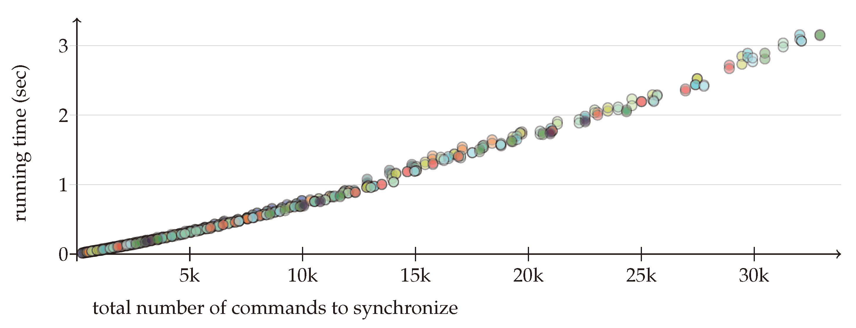
In the experiments, we tried 20 different filesystems with the parameter S running from 5 to 14 (inclusive), T running from 1 to $\left[\right(S-1)/2]$, and the number of users running from 2 to $S-1$, inclusive. The general synchronization Algorithm 7 from Section 6 was called on the resulting collection of sequences to generate the first and the first three possible synchronized states. Each run was repeated 10 times to smooth out the effects of other programs running on the same server. Figure 3 depicts the average time used to generate a single synchronizing command set. The input size on the x axis is the total number of different commands in the sequences to be synchronized. The average running time on the y axis is in seconds. The non-optimized Python program was running on a desktop machine with an Intel(R) Core(TM) i5-8250U CPU @ 1.60 GHz processor and 8 G memory. The different colors represent the number of replicas. The results confirm that the running time is subquadratic in the total input size and does not depend on the number of replicas.

8. Conclusions

This paper presented a provably correct synchronization algorithm running in subquadratic time, which can synchronize an arbitrary number of replicas. The existence of such an algorithm was a long-standing open problem [12] in the fields of operation transformation (OT) [5] and conflict-free replicated data types (CRDT) [9]. Our work is based on the algebraic theory of filesystems (ATF) [14], which, in many respects, resembles both OT and CRDT. Instead of traditional filesystem commands, ATF uses operations enriched with contextual information similarly to OT and CRDT. It also favors commutativity, but instead of requesting all operations to be commutative, their non-commutative part can be isolated systematically and handled separately. As a consequence, similarly to OT and CRDT, ATF can deal with command sets instead of sequences, where the execution order is not specified, but the semantics of executing the commands in some order is defined unambiguously.

The underlying filesystem model, while arguably simplistic, retains the most important high-level and platform-independent properties of real-life filesystems; see Section 2.1 for a more detailed discussion. The two most prominent omissions of this model are the lack of directory attributes (the model handles all directories as equal), and links breaking the regular tree-like structure of filesystem paths. Both of these shortcomings, and how to circumvent them, are discussed below.

Filesystem synchronization starts with update detection run locally, which extracts information encoding the state of the modified replica as discussed in Section 3.1. In the ATF framework, this information is a canonical command set describing how to construct the replica from the original filesystem.

The task of the synchronizer is to create a common, merged filesystem after considering what changes have been applied to the replicas. In the ATF framework, this task amounts to creating another canonical command set, the merger, which transforms the original filesystem into the merged filesystem. What this merger can be is described by two simple and intuitively appealing principles: the intention-confined effect, where operations in the merger should come from those supplied by the replicas, and aggressive effect preservation, where the merger should contain as many of those commands as possible. Definition 5 formalizes this idea and defines what a synchronized state is. Section 3.3 and Section 3.5 discuss that this goal-driven definition automatically implies many operational properties such that a merger command set always defines a valid synchronized state; synchronization can be achieved from the local copy by rolling back some of the local commands and executing additional ones originating from other replicas. Section 3.7 shows that with minimal effort the synchronization paradigm can be extended to tolerate replicas which do not lock their filesystem—allowing for asynchronous or optimistic synchronization [9]. Even replicas missing a synchronization cycle can later upgrade to the synchronized state.

Algorithms described in Section 4 give a high-level description of a proof-of-concept implementation at https://github.com/csirmaz/algebraic-reconciler (accessed on 10 May 2023). Algorithm 5 creates a merger in linear time after sorting the canonical sets sent by the replicas. While this algorithm can make some nondeterministic decisions, it cannot generate all possible mergers. Two nondeterministic algorithms which can do so are sketched in Section 6; both of them run in near linear time. The first algorithm uses the fact that Algorithm 5 can recognize mergers. It first creates a random subset of the supplied commands blindly, and then checks if it is a merger. The second one, described as Algorithm 7, is more elaborate. It exploits the structure of refluent command sets, and can assist in the synchronization process by highlighting the consequences of different conflict resolutions.

8.1. Node Attributes

The important task of consolidating different versions of the same document (file value) was not considered, as processing the internal structure of file contents is outside the scope of filesystem synchronization. Files different in content are considered to be different, and the synchronization algorithm forces the choosing of one or the other. There is, however, an easy way of incorporating third-party content-merging applications. This can be done by pretending that there is only one possible file content, and using the ATF framework to synchronize the structure of the filesystems. When it becomes clear which nodes contain file values, check for the commands which modified the actual content there, and use the external application to determine the final file content. A similar approach can handle node attributes by considering the changes made by the replicas at some node and consolidating them. This approach, however, should be followed carefully. To illustrate the problem, consider a directory at node n, which originally had the “private” attribute. Replica A changes this attribute to “public”, while replica B, under the impression that the directory is private, creates a file under it. When merging the attributes, the change at node n is carried over, making the directory publicly available. This, however, is clearly unacceptable. It is an interesting open problem to incorporate node attributes into the ATF synchronization paradigm.

8.2. Filesystems on Directed Acyclic Graphs

From the user’s perspective, a (hard or soft) link between the nodes n and $n^{\prime }$ is a promise, or a commitment, that the filesystem at and below n is exactly the same at and below $n^{\prime }$. In other words, the filesystem acts as if the nodes n and $n^{\prime }$ in the filesystem skeleton are glued together.

If the filesystem has many links and the links do not form loops, then after this gluing, the skeleton becomes a directed acyclic graph (DAG) with many sources (the roots in the original skeleton). The gluing works in the other direction, too: given any DAG with one or more sources, it can be “unfolded” into a forest. The paths of a tree-like filesystem can be identified with the directed paths starting from a source, and two nodes are “linked” if the directed paths in the DAG lead to the same vertex. A DAG vertex v represents the collection of all nodes in the unfolded filesystem, which are determined by the directed paths in the DAG, which lead to v. Two nodes of this unfolded filesystem are equivalent, written as $n_1\simeq n_2$ if the corresponding directed DAG paths lead to the same vertex. It is clear that ≃ is an equivalence relation, and factoring the filesystem by ≃ yields the DAG. If every vertex in the DAG has a finite indegree, then the equivalence classes are also finite.

Operations on a DAG-based filesystem can be mimicked on the unfolded filesystem by simply requesting that an operation performed on the DAG vertex v be done on all nodes represented by v. Similarly, a command set A on the unfolded filesystem corresponds to the command set $A/\simeq$ on the DAG-based filesystem if with every command $\sigma \in A$ all commands ≃-equivalent to $\sigma$ are also in A. We call these command sets ≃-invariant. Requesting all command sets to be ≃-invariant, the claims, propositions and theorems in this paper remain true (remark that in this case, the definition of a merger should require M to be ≃-invariant). Similarly, all algorithms continue to work, but they must handle not commands but sets of ≃-equivalent commands. Consequently, time estimates are no longer valid. In summary, our results and algorithms remain valid on filesystems based on arbitrary DAGs. It is an open question as to whether the algorithms can be implemented in linear time in the general case.

References

- Athow, D.; Turner, B. Best File Syncing Solutions of 2023. 2023. Available online: https://www.techradar.com/best/best-file-syncing-solution (accessed on 10 May 2023).
- Mościcki, J.T.; Mascetti, L. Cloud storage services for file synchronization and sharing in science, education and research. Future Gener. Comput. Syst. 2018, 78, 1052–1054. [Google Scholar] [CrossRef]
- Sun, C.; Jia, X.; Zhang, Y.; Yang, Y.; Chen, D. Achieving Convergence, Causality Preservation, and Intention Preservation in Real-Time Cooperative Editing Systems. ACM Trans. Comput. Hum. Interact. 1998, 5, 63–108. [Google Scholar] [CrossRef]
- Sun, C.; Ellis, C.A. Operational Transformation in Real-Time Group Editors: Issues, Algorithms, and Achievements. In Proceedings of the ACM 1998 Conference on Computer Supported Cooperative Work, Seattle, WA, USA, 14–18 November 1998; Poltrock, S.E., Grudin, J., Eds.; ACM: New York, NY, USA, 1998; pp. 59–68. [Google Scholar] [CrossRef]
- Shao, B.; Li, D.; Lu, T.; Gu, N. An Operational Transformation Based Synchronization Protocol for Web 2.0 Applications. In Proceedings of the ACM 2011 Conference on Computer Supported Cooperative Work, Hangzhou, China, 19–23 March 2011; CSCW ’11. Association for Computing Machinery: New York, NY, USA, 2011; pp. 563–572. [Google Scholar] [CrossRef]
- Ng, A.; Sun, C. Operational Transformation for Real-time Synchronization of Shared Workspace in Cloud Storage. In Proceedings of the 19th International Conference on Supporting Group Work, Sanibel Island, FL, USA, 13–16 November 2016; Lukosch, S.G., Sarcevic, A., Lewkowicz, M., Muller, M.J., Eds.; ACM: New York, NY, USA, 2016; pp. 61–70. [Google Scholar] [CrossRef]
- Day-Richter, J. What’s Different about the New Google Docs: Making Collaboration Fast. 2010. Available online: https://drive.googleblog.com/2010/09/whats-different-about-new-google-docs.html (accessed on 12 January 2023).
- Shapiro, M.; Preguiça, N.M.; Baquero, C.; Zawirski, M. Conflict-Free Replicated Data Types. In Proceedings of the Stabilization, Safety, and Security of Distributed Systems-13th International Symposium, SSS 2011, Grenoble, France, 10–12 October 2011; Défago, X., Petit, F., Villain, V., Eds.; Springer: Berlin/Heidelberg, Germany, 2011; Volume 6976, pp. 386–400. [Google Scholar] [CrossRef]
- Preguiça, N.M. Conflict-free Replicated Data Types: An Overview. arXiv 2018, arXiv:1806.10254. [Google Scholar]
- Tao, V.; Shapiro, M.; Rancurel, V. Merging semantics for conflict updates in geo-distributed file systems. In Proceedings of the 8th ACM International Systems and Storage Conference, SYSTOR 2015, Haifa, Israel, 26–28 May 2015; Naor, D., Heiser, G., Keidar, I., Eds.; ACM: New York, NY, USA, 2015; pp. 1–12. [Google Scholar] [CrossRef]
- Liu, E. A CRDT-Based File Synchronization System. Master’s Thesis, Norwegian University of Science and Technology, Trondheim, Norway, 2021. [Google Scholar]
- Shekow, M. Syncpal: A Simple and Iterative Reconciliation Algorithm for File Synchronizers. Ph.D. Thesis, RWTH Aachen University, Aachen, Germany, 2019. [Google Scholar]
- Csirmaz, E.P. Algebraic File Synchronization: Adequacy and Completeness. arXiv 2016, arXiv:1601.01736. [Google Scholar]
- Csirmaz, E.P.; Csirmaz, L. Data Synchronization: A Complete Theoretical Solution for Filesystems. Future Internet 2022, 14, 344. [Google Scholar] [CrossRef]
- Shapiro, M.; Preguiça, N.; Baquero, C.; Zawirski, M. A Comprehensive Study of Convergent and Commutative Replicated Data Types; Technical Report 7506; INRIA, Inria-Centre Paris-Rocquencourt: Le Chesnay-Rocquencourt, France, 2011. [Google Scholar]
- Knuth, D.E. The Art of Computer Programming, Vol. 1: Fundamental Algorithms, 3rd ed.; Addison-Wesley: Boston, MA, USA, 1997. [Google Scholar]
- Balasubramaniam, S.; Pierce, B.C. What is a File Synchronizer? In Proceedings of the MOBICOM ’98, The Fourth Annual ACM/IEEE International Conference on Mobile Computing and Networking, Dallas, TX, USA, 25–30 October 1998; Osborne, W.P., Moghe, D.B., Eds.; ACM: New York, NY, USA, 1998; pp. 98–108. [Google Scholar] [CrossRef]
- Tridgell, A.; Mackerras, P. The Rsync Algorithm; Australian National University: Canberra, Australia, 1996. [Google Scholar]
- Boškov, N.; Trachtenberg, A.; Starobinski, D. Enabling Cost-Benefit Analysis of Data Sync Protocols. arXiv 2023, arXiv:2303.17530. [Google Scholar]
- Preguiça, N.; Marques, J.M.; Shapiro, M.; Letia, M. A Commutative Replicated Data Type for Cooperative Editing. In Proceedings of the 2009 29th IEEE International Conference on Distributed Computing Systems, Montreal, QC, Canada, 22–26 June 2009; ICDCS ’09. IEEE Computer Society: Washington, DC, USA, 2009; pp. 395–403. [Google Scholar] [CrossRef]
- Antkiewicz, M.; Czarnecki, K. Design Space of Heterogeneous Synchronization. In Proceedings of the Generative and Transformational Techniques in Software Engineering II: International Summer School, GTTSE 2007, Braga, Portugal, 2–7 July 2007; Revised Papers. Lämmel, R., Visser, J., Saraiva, J., Eds.; Springer: Berlin, Heidelberg, 2008; pp. 3–46. [Google Scholar] [CrossRef]
- Li, Z.; Wilson, C.; Jiang, Z.; Liu, Y.; Zhao, B.Y.; Jin, C.; Zhang, Z.L.; Dai, Y. Efficient Batched Synchronization in Dropbox-Like Cloud Storage Services. In Proceedings of the Middleware 2013, Beijing, China, 9–13 December 2013; Eyers, D., Schwan, K., Eds.; Springer: Berlin, Heidelberg, 2013; pp. 307–327. [Google Scholar]
- Petroni, A.; Cuomo, F.; Schepis, L.; Biagi, M.; Listanti, M.; Scarano, G. Adaptive Data Synchronization Algorithm for IoT-Oriented Low-Power Wide-Area Networks. Sensors 2018, 18, 4053. [Google Scholar] [CrossRef] [PubMed]
- Feng, J.; Qiao, X.; Li, Y. The research of synchronization and consistency of data in mobile environment. In Proceedings of the 2012 IEEE 2nd International Conference on Cloud Computing and Intelligence Systems, Hangzhou, China, 30 October–1 November 2012; Volume 2, pp. 869–874. [Google Scholar] [CrossRef]
- Klophaus, R. Riak Core: Building Distributed Applications without Shared State. In Proceedings of the ACM SIGPLAN Commercial Users of Functional Programming, Baltimore, MD, USA, 1–2 October 2010; CUFP ’10. Association for Computing Machinery: New York, NY, USA, 2010. [Google Scholar] [CrossRef]
- Qian, Y. Data Synchronization and Browsing for Home Environments. Ph.D. Thesis, Technische Universiteit Eindhoven, Eindhoven, The Netherlands, 2004. [Google Scholar] [CrossRef]
- Zhang, Y.; Dragga, C.; Arpaci-Dusseau, A.; Arpaci-Dusseau, R. *-Box: Towards Reliability and Consistency in Dropbox-like File Synchronization Services. In Proceedings of the 5th USENIX Conference on Hot Topics in Storage and File Systems, Renton, WA, USA, 8–9 July 2019; HotStorage’13. USENIX Association: Berkeley, CA, USA, 2013; p. 2. [Google Scholar]
- Even, S. Graph Algorithms, 2nd ed.; Cambridge University Press: Cambridge, UK, 2011. [Google Scholar] [CrossRef]
Figure 1.
The synchronization cycle. Identical copies of the same filesystem are edited independently. Each replica sends the locally created update information to the synchronizer, which returns the commands to be executed on the local copy to update it to a common synchronized state.
Figure 2.
Asynchronous synchronization. Top line: after the synchronization request has been sent, additional local modifications are made to the filesystem. When receiving the synchronization commands, they are modified using the current state of the local filesystem. Bottom line: the end result should be the same as applying the synchronization commands immediately and then making the local modifications afterwards.
Figure 3.
Running time for generating the synchronized state on several synthetic data sets. The running time depends only on the total number of filesystem commands (x axis), and not on the number of replicas (color).
Disclaimer/Publisher’s Note: The statements, opinions and data contained in all publications are solely those of the individual author(s) and contributor(s) and not of MDPI and/or the editor(s). MDPI and/or the editor(s) disclaim responsibility for any injury to people or property resulting from any ideas, methods, instructions or products referred to in the content. |
© 2023 by the authors. Licensee MDPI, Basel, Switzerland. This article is an open access article distributed under the terms and conditions of the Creative Commons Attribution (CC BY) license (https://creativecommons.org/licenses/by/4.0/).
Share and Cite
MDPI and ACS Style
Csirmaz, E.P.; Csirmaz, L. Synchronizing Many Filesystems in Near Linear Time. Future Internet 2023, 15, 198. https://doi.org/10.3390/fi15060198
AMA Style
Csirmaz EP, Csirmaz L. Synchronizing Many Filesystems in Near Linear Time. Future Internet. 2023; 15(6):198. https://doi.org/10.3390/fi15060198
Chicago/Turabian StyleCsirmaz, Elod P., and Laszlo Csirmaz. 2023. "Synchronizing Many Filesystems in Near Linear Time" Future Internet 15, no. 6: 198. https://doi.org/10.3390/fi15060198
Note that from the first issue of 2016, this journal uses article numbers instead of page numbers. See further details here.