Data Protection and Multi-Database Data-Driven Models

Abstract

Anonymization and data masking have effects on data-driven models. Different anonymization methods have been developed to provide a good trade-off between privacy guarantees and data utility. Nevertheless, the effects of data protection (e.g., data microaggregation and noise addition) on data integration and on data-driven models (e.g., machine learning models) built from these data are not known. In this paper, we study how data protection affects data integration, and the corresponding effects on the results of machine learning models built from the outcome of the data integration process. The experimental results show that the levels of protection that prevent proper database integration do not affect machine learning models that learn from the integrated database to the same degree. Concretely, our preliminary analysis and experiments show that data protection techniques have a lower level of impact on data integration than on machine learning models.

1. Introduction

When personal data are used, we need to take into account privacy requirements. Current national and international regulations require companies to take privacy requirements seriously; see, e.g., GDPR, under which companies can be fined when disclosure of sensitive data takes place. Data cannot be shared freely with third parties when there is sensitive information. Nevertheless, it is not only the data that needs to satisfy privacy requirements, but also data-driven models built from these sensitive data. Privacy-by-design [1] states that privacy is not an add-on to systems processing data, but that privacy needs to be taken into account as a fundamental requirement of all the processes.

Privacy technologies [2,3,4] have been developed to provide solutions that permit the sharing of data as well as building data-driven models that are compliant with our privacy requirements. There exist several privacy models, computational definitions of privacy, and alternative data protection mechanisms to implement the privacy models. Masking methods are tools that allow the data to be protected so that they can be shared with third parties without compromising sensitive data. Masking methods modify the original data, providing a sanitized version of a file or database, so that these sensitive data are not disclosed, and disclosure risk is minimized. As masking methods modify the original data, data utility is a major concern. Masking methods are typically parametric so that we can control the privacy level, or at least the perturbation level.

The effects of masking methods on machine learning and statistics have been extensively studied [5,6,7]. A typical analysis consists of evaluating how different privacy levels affect the performance of data-driven models. This includes discovering which range of parameters results in an acceptable performance (e.g., accuracy or error) and which range of parameters causes the model to show unacceptable performance. Additionally, masking methods [8] have been compared in terms of performance for similar protection. Most of these comparisons are computational, testing the performance of the methods for particular data sets and particular machine learning algorithms.

There is an increasing need to build more complex data-driven models. There is a need to use data from multiple databases, and once these data are integrated, data-driven models are built from the resulting databases. The effects of masking methods on data when these data are to be integrated is not known. In this paper, we study this problem. More specifically, we want to know

• to what extent data integration is possible when data have been masked, and
• even if data integration cannot overcome the errors caused by masking methods and produces faulty databases, we want to know whether these databases are of high enough quality for data-driven models to be built.

To achieve this goal, we conduct a series of controlled experiments. More precisely, given a database, we produce two different partial databases, which are protected separately and later integrated. Then, data-driven models are built from the integrated database. The results of the process are analyzed. We study the effects of different masking methods on different databases. We also consider the performance of alternative machine learning models. This paper is an extended version of a conference paper [9]. The paper is completely rewritten and we extend the experiments with additional databases, masking methods, parameterizations, and machine learning models. In fact, the software used for preparing this paper is also new, as previous experiments were performed in R and these ones were carried out in Python. A description of the software and a link to it are included below.

The structure of the paper is as follows. In Section 2, we describe the main concepts we need in our paper. In Section 3 we present the methodology used. We formalize the process applied to a given database. We also describe the masking methods applied, the machine learning algorithms considered, and the databases used in the experiments. In Section 4, we present our main results and our analysis. The paper finishes with conclusions and research directions.

2. Preliminaries

Data protection mechanisms are used when we need to share data with third parties. There are three main types of mechanisms [3,4]: perturbative methods, non-perturbative methods, and synthetic data generators.

Perturbative methods build a copy of the database in which the original data have been modified by introducing some kind of error. There are several algorithms with this goal. Examples include microaggregation, noise addition and multiplication, rank swapping, PRAM (Post RAndomisation Method), and transformation-based methods. In this paper, we use this type of method for protecting data. Different methods provide different guarantees and protection. For example, microaggregation is useful for providing k-anonymity [10,11,12]. In contrast, noise addition using Laplacian noise is useful for providing local differential privacy [13,14,15]. All methods are useful for providing privacy against reidentification [16] attacks.

Non-perturbative methods build a copy of the database in which the original data are replaced by data of lower quality. Here, data are not erroneous but may lack detail. E.g., values can be replaced by intervals, or simply suppressed. Different methods may provide different privacy guarantees (e.g., k-anonymity). Nevertheless, as the type of data after protection is different to the type of data before protection, perturbative methods are easier to use. For example, the original data may be numerical but protected data may correspond to intervals. Therefore, we need to use machine learning algorithms that are able to deal with intervals (or alternatively post-process the data to replace intervals with values). For this reason, we have not used these methods here.

Synthetic data generators [17] are based on building models of the data, and then data are replaced by artificial data generated by these models. Different methods exist, typically based on different machine learning models (e.g., generative adversarial networks, decision trees, support vector machines). We have not considered these approaches here, and we leave the analysis of this type of method for future work.

3. Methodology

As we have stated in the introduction, our main goal is to evaluate to what extent masking methods affect data-driven models built after data integration. Here, we understand data-driven models as models that have learnt from data using machine learning algorithms. In our analysis, we take two aspects into account. One is about the data integration process itself. That is, we want to analyze whether masking affects the integration process itself. The second aspect relates to data-driven models built from integrated data. That is, we want to analyze the quality of data-driven models built from data after the integration process.

In order to assess both the data integration process and the data-driven model, we have used the following methodology. This methodology is based on the one described in our previous paper [9]. As we explain in the next section, in this paper we have a deeper analysis as we compare more masking methods, more machine learning algorithms, and more data sets.

This work is based on existing techniques in data protection, data integration and machine learning models. In particular, we analyze data protection strategies on data integration and their corresponding impacts passed on to machine learning models. A detailed step-by-step description of the methodology is given below. We begin with a single database, which we denote $D{B}_0$. A fraction of the records of this database are vertically partitioned into two different databases. These two databases are not disjoint, but they share some attributes. The purpose of this is to allow us to consider database integration and enable us to analyze the effects of masking methods on database integration.

In addition to the database $D{B}_0$, the methodology also requires a masking method $\rho$, a machine learning algorithm m, and a database integration method $\mathit{integrate}$. We will denote by y the dependent attribute in the database, and $y\left(x\right)$ is the value of this attribute for record x in the database (without the attribute y itself).

Our methodology is as follows:

• Partition $D{B}_0$ horizontally into two parts, one for testing and the other for training. We call the training part $DB$ and the testing part $D{B}_t$.
• Take $DB$ and partition it vertically into two databases, $D{B}_1$ and $D{B}_2$. These two databases will share some attributes. We denote by $nC$ the number of attributes that are shared by both databases.
• Let $\rho$ be a masking method. Independently mask the two databases $D{B}_1$ and $D{B}_2$. In this way, we produce two masked databases as follows: $D{B}_1^{\prime }=\rho \left(D{B}_1\right)$ and $D{B}_2^{\prime }=\rho \left(D{B}_2\right)$.
• Integrate $D{B}_1^{\prime }$ and $D{B}_2^{\prime }$ using the $nC$ common attributes of these databases. We denote by $D{B}^{\prime }$ the resulting database. That is, $D{B}^{\prime }=\mathit{integrate}(D{B}_1^{\prime },D{B}_2^{\prime })$ where $\mathit{integrate}$ is an integration mechanism for databases.
• Let m denote a machine learning algorithm. Compute a data-driven model for $DB$ and another data-driven model for $D{B}^{\prime }$ using the same machine learning algorithm. We denote by $m\left(DB\right)$ and $m\left(D{B}^{\prime }\right)$ these two different data-driven models. We use $m\left(DB\right)\left(x\right)$ to denote the application of this model to a record x from $DB$ (not including the attribute y).
• Evaluate the integration of the two databases (that is, the resulting database $D{B}^{\prime }$) using $DB$.
• Evaluate the performance of the models $m\left(DB\right)$ and $m\left(D{B}^{\prime }\right)$ using the test database $D{B}_t$.

In order to make this process concrete, some steps need further clarification. We will describe them below.

First, the database integration process: for this purpose we have used distance-based record linkage [18,19]. This is one of the most effective algorithms, and at the same time, it is simple to apply. Given a record $r_1$ in $D{B}_1^{\prime }$, we compute its distance to each record $r_2$ in $D{B}_2^{\prime }$. Then, we select the most similar one $r^{\prime }\left(r_1\right)$ to $r_1$. Formally, this corresponds to $r^{\prime }\left(r_1\right)=arg{min}_{r_2\in D{B}_2^{\prime }}d(r_1,r_2)$. Distance-based record linkage needs a distance function d. We have used the Euclidean distance, which uses and compares the common attributes in both databases $D{B}_1^{\prime }$ and $D{B}_2^{\prime }$. So, $d(r_1,r_2)$ uses only the common attributes of records $r_1$ and $r_2$ (i.e., $nC$ attributes). It is important to note that for the database integration process, we know how $D{B}_1^{\prime }$ and $D{B}_2^{\prime }$ have been generated, and we know which attributes in one database correspond to which attributes in the other database. Therefore, in our case, the database integration process does not need to take into account attribute alignment nor schema matching. More complex situations can be envisioned in the context of data privacy, in line with the above mentioned references and with [4] (Appendix A).

We have considered two different types of evaluations for the database integration process. One relates to the result of the integration process itself. Note that both databases, $D{B}_1^{\prime }$ and $D{B}_2^{\prime }$, are generated from a single database $DB$ through its partition and the subsequent process of masking the two parts. Because of this, we can evaluate to what extent the database $D{B}^{\prime }=\mathit{integrate}(D{B}_1^{\prime },D{B}_2^{\prime })$ is correctly integrated by means of considering whether the record linkage aligns the records $r_1$ and $r_2$ correctly. To do so, we count how many times $r^{\prime }\left(r_1\right)$ is the correct link in $D{B}_2^{\prime }$ for $r_1$. As we will discuss in Section 4, the number of correct links drops very quickly with respect to the data protection level. In other words, most of the links we compute using distance-based record linkage are incorrect.

The other evaluation is related to the models built from the databases. Even if the databases are not correctly integrated, we can consider whether the model we build is good enough (or similar enough in terms of performance) compared with the model we build using the original data; that is, a comparison between $m\left(DB\right)$ for a record x (i.e., $m\left(DB\right)\left(x\right)$) and $y\left(x\right)$. As we solely use numerical data, we use for this evaluation the prediction of the models for the records in the testing database (i.e., $D{B}_t$). We compute the sum of squared errors of both $m\left(DB\right)$ and $m\left(D{B}^{\prime }\right)$ and compare them. Formally, our evaluation of both models uses the following expression, which is about zero when the error is similar for both types of models. Note that we keep the sign in the difference (no squared numerator, no absolute value in the numerator). Therefore, if the model built from the masked data performs worse than the model built from the original data, the evaluation is positive. This is what we would expect, and what we see in the experiments. Nevertheless, if the performance of the model built from the masked data is better than the model built from the original database, then the evaluation would be negative. We have observed this situation only a few times in our experiments, which is consistent with other results in the literature. For example, it has been observed when masking single databases (see, e.g., the work by Sakuma and Osame [20] and by Aggarwal and Yu [21]). Because of this, we consider that it is better to define the expression by keeping the sign. That is,

$$ev(D{B}_t,D{B}^{\prime })=\frac{{\sum }_{x\in D{B}_t}{\left(m\left(DB\right)\left(x\right)-y\left(x\right)\right)}^2-{\left(m\left(D{B}^{\prime }\right)\left(x\right)-y\left(x\right)\right)}^2}{|D{B}_t|}$$

(1)

If we consider the process as a whole, we also need to describe the masking methods and the algorithms used to compute the machine learning model. We have used several masking methods and several machine learning algorithms, which are described below.

3.1. Masking Methods

We have considered methods for microaggregation (MDAV and Mondrian algorithms), noise addition (both Gaussian and Laplacian noise), two methods based on dimensionality reduction (SVD and PCA), and another method based on non-negative matrix factorization. We briefly describe the methods below. These masking methods are described in detail in books on data privacy [3,4].

• Microaggregation: in order to protect a set of records, small clusters are built and records are replaced by a cluster representative. In order to guarantee privacy, each cluster needs to have at least k records. Thus, k is a parameter of the method. The larger the k, the larger the privacy level, and the lower the utility of the data. Optimal microaggregation is often defined in terms of the error between the cluster representatives and the original records. Optimal microaggregation is an NP-hard problem for multivariate data (see e.g., [22]). Because of this, several alternative heuristic algorithms have been developed. We have used two alternative algorithms: MDAV [23,24], and Mondrian [25]. The difference is related to the method of building the clusters. We use the mean of the records in a cluster as the cluster representative. Microaggregation provides k-anonymity by definition, as each record in the protected data set is indistinguishable from at least $k-1$ other records.
• Noise addition: in order to protect a record, noise is added to it. In other words, the original numerical value x is replaced by $x+ϵ$, where $ϵ$ follows a given distribution. We use two different alternative distributions for protection. They are a normal distribution with mean zero and standard deviation $\sqrt{(}\mathit{variance}*k)$, and a Laplace distribution with mean zero and standard deviation as above. Naturally, k corresponds to the parameter of the method. As in the case of microaggregation, the larger the k, the larger the distortion. Therefore, the larger the k, the larger the protection and the smaller the utility of the resulting protected data. Noise addition using Laplacian noise is the standard approach to implementing differential privacy. In the case of publishing a database, as we do here, this corresponds to local differential privacy.
• Transform-based protection: these methods reduce the quality of the data by transforming the data into another space in which we can remove details. We have considered the use of singular value decomposition (SVD), principal component analysis (PCA), and non-negative matrix factorization (NMF) for this purpose. In the case of SVD and PCA, we apply the decomposition, select the principal components, and then we rebuild the matrix with only these selected components. The parameter of the method is the number of components selected. We denote this k. In this case, the larger the k, the better the reconstruction of the original data. Therefore, the smaller the k, the larger the protection, and at the same time, the smaller the utility of the resulting protected data. This approach is similar to non-negative matrix factorization. For NMF, as above, the smaller the number of components k, the larger the protection and the smaller the utility. While SVD and PCA can be applied to matrices with arbitrary real numbers, NMF can only be applied to positive data. Because of this, data are scaled into the [0,1] interval before the application of the NMF protection. The data are re-scaled back after the NMF protection.

3.2. Machine Learning Algorithms

We have restricted our study to numerical data. Therefore, we used regression algorithms. We used four regression algorithms among the ones supplied by the Python package sklearn. We selected these methods because we consider them to be quite representative regression methods, and we had already used them in a previous work of ours [26] (on the effects of masking in some explainability tools). All methods were applied using their default parameters. The methods considered are the following:

• linear_model.LinearRegression (linear regression): a linear approach to modeling the relationship between a dependent variable and one or more independent variables.
• sklearn.linear_model.SGDRegressor (SGD regression): a linear regression model fitted by minimizing a regularized empirical loss with stochastic gradient descent.
• sklearn.kernel_ridge.KernelRidge (kernel ridge regression): a regression model combining ridge regression (imposing a penalty with l2 regularization) with the kernel trick. It can model linear and nonlinear relationships between a dependent variable and one or more independent variables.
• sklearn.svm.SVR (epsilon-support vector regression): a regression model using the same principles (e.g., maximal margin) as the SVM for classification. One difference is that a margin of tolerance (epsilon) is set.

3.3. Implementation

We implemented our methodology in Python. We used our own implementations of masking methods and of database integration (i.e., a distance-based record linkage algorithm). These implementations are publicly available [27]. Machine learning algorithms were selected from the ones available in sklearn.

3.4. Databases

We considered the following databases. Two of them are provided by the sdcMicro [28] package in R, which provides tools for database protection. Among the tools, there are masking methods and data sets that have been used to compare the performance of masking methods with respect to disclosure risk and utility.

• CASC: this data set has been used in several papers on data privacy, and it is provided by the sdcMicro package in R (it is called CASCrefmicrodata in the package). The data set was created in the EU project CASC. See, e.g., Hundepool et al. [3] and the sdcMicro package description for detailed information on this data set. The data set consists of 1080 records and 13 numerical attributes.
• Tarragona: this data set is also provided by the sdcMicro package in R. There are 834 records described in terms of 13 numerical attributes.
• Concrete Compressive Strength: this data set is described by Yeh [29,30] and has been used in several works related to regression models. It is provided by the UCI repository. The data set consists of 1030 records and 9 numerical attributes. We have selected this file because the data are numerical and because it has been used for regression.

3.5. Parameters

The data sets were partitioned into test and training sets. Our partition randomly assigns 80% of the records for training and the remaining 20% of the records for testing.

Next, we vertically partitioned training data into two databases. This corresponds to building the two databases $D{B}_1$ and $D{B}_2$, which will share a set of attributes. The selection of the attributes depends on the database. They are as follows:

• CASC: The number of common attributes for $D{B}_1$ and $D{B}_2$ considered is $nC=1,2,3,4,5,6$. That is, we considered six different pairs of databases. These databases were built as follows. For the first pair, $D{B}_1$ includes attributes 0–5, and $D{B}_2$ includes attributes 5–11 (0–5 and 5–11 correspond to columns in the database, with the first column denoted by zero). Databases $D{B}_1$ for $nC=2,\dots ,6$ are defined in terms of attributes 0–6, 0–6, 0–7, 0–7, and 0–7. Databases $D{B}_2$ for $nC=2,\dots ,6$ are defined with attributes 5–11, 4–11, 4–11, 3–11, and 2–11.
• Tarragona: The number of common attributes is the same as for the CASC data set, and the databases were also constructed following the same pattern.
• Concrete: In this case, we also have $nC=1,\dots ,6$. For $nC=1$, we have $D{B}_1$ with attributes 0–5 and $D{B}_2$ with attributes 5–7. For $nC=2$, we have $D{B}_1$ with attributes 0–6 and $D{B}_2$ with attributes 5–7. For larger $nC$, we have $D{B}_1$ with attributes 0–6, 0–7, 0–7, and 0–7, and $D{B}_2$ with attributes 4–7, 4–7, 3–7, and 2–7.

Masking methods were applied considering different parameterizations. The following parameterizations have been considered.

• Microaggregation (MDAV and Mondrian). The following values of k were considered: $k=\{2,3,4,5,6,7,8,9,10,12,14,15,16,18,20\}$. For some experiments, we used larger values. In that case, we used $k=\{2,4,6,8,10,15$, 20, 25, 30, 40, 50, 60, 70, 100, 200, 300, 400, $500\}$.
• Noise addition (Gaussian and Laplacian noise). We used noise with parameters in the set $\{0.2,0.3,0.4,0.5,0.6,0.7,0.8,0.9,1.0,1.2,1.4,1.5\}$.
• SVD and NMF. In this case, we used parameters equal to $\{2,3,4,5,6,7,8\}$.
• PCA. We used one, two, and three principal components.

Machine learning algorithms were used with their standard parameters. No tuning was applied. As explained above, we used the sklearn Python package. Regression models were used because all data were numerical. The dependent attribute for each database is discussed above.

4. Experiment and Analysis

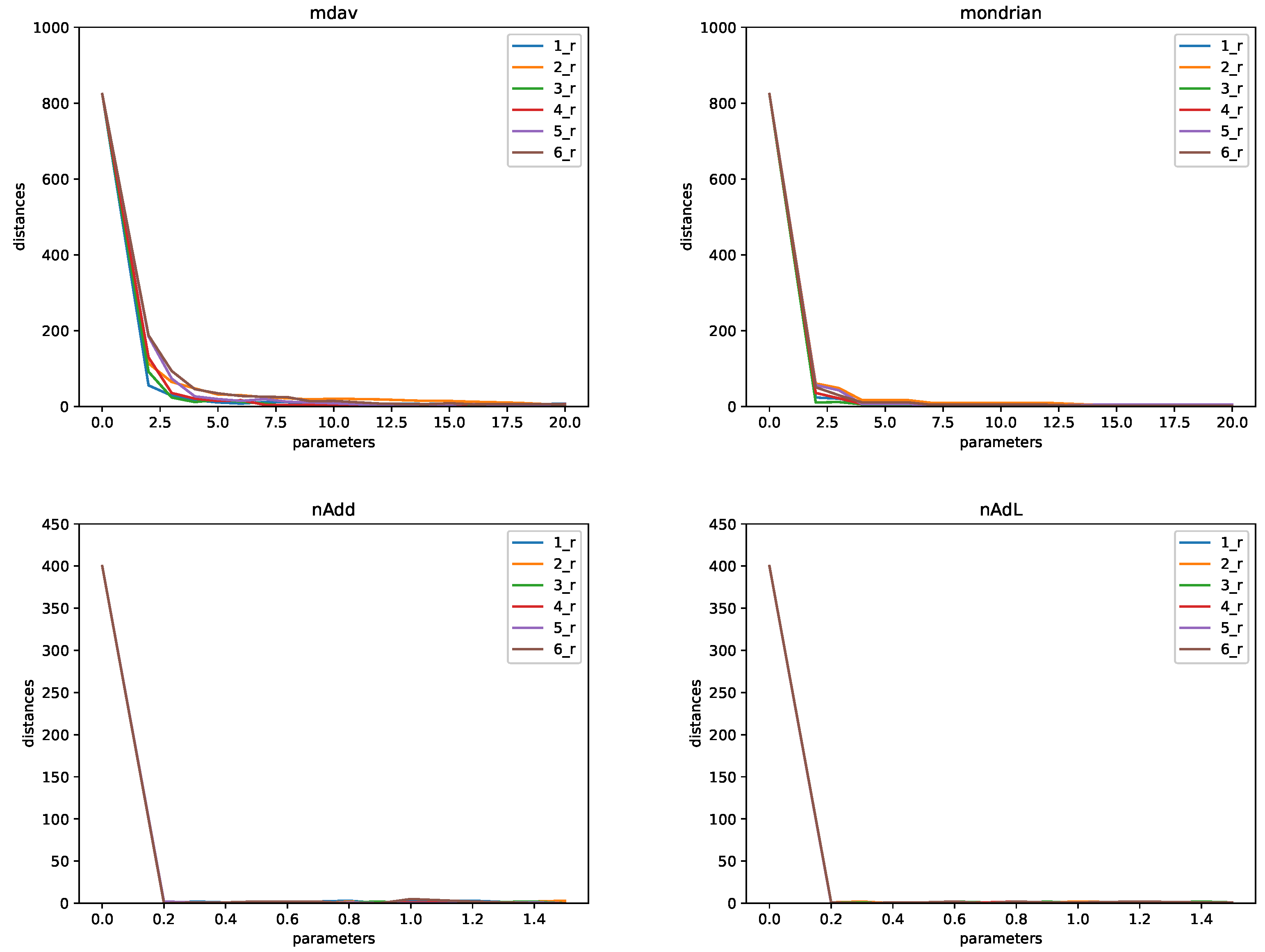
The experiments show that when we integrate two masked protected files, the number of correct reidentifications degrades very quickly for most masking methods. That is, the number of records that are correctly linked (i.e., one record in one file is associated with the right record in the other file) is very small, even for parameters providing very low protection. This holds for most masking methods except for the ones based on SVD and NMF, which have, in general, quite large reconstruction rates when the number of singular values is high and when the number of components is high.

Figure 1 illustrates the case of microaggregation (MDAV, Mondrian), and noise addition (Gaussian and Laplacian noise). When their parameters are equal to zero, there is no protection. Here, we see that even with six common attributes, the number of reidentifications decreases very rapidly.

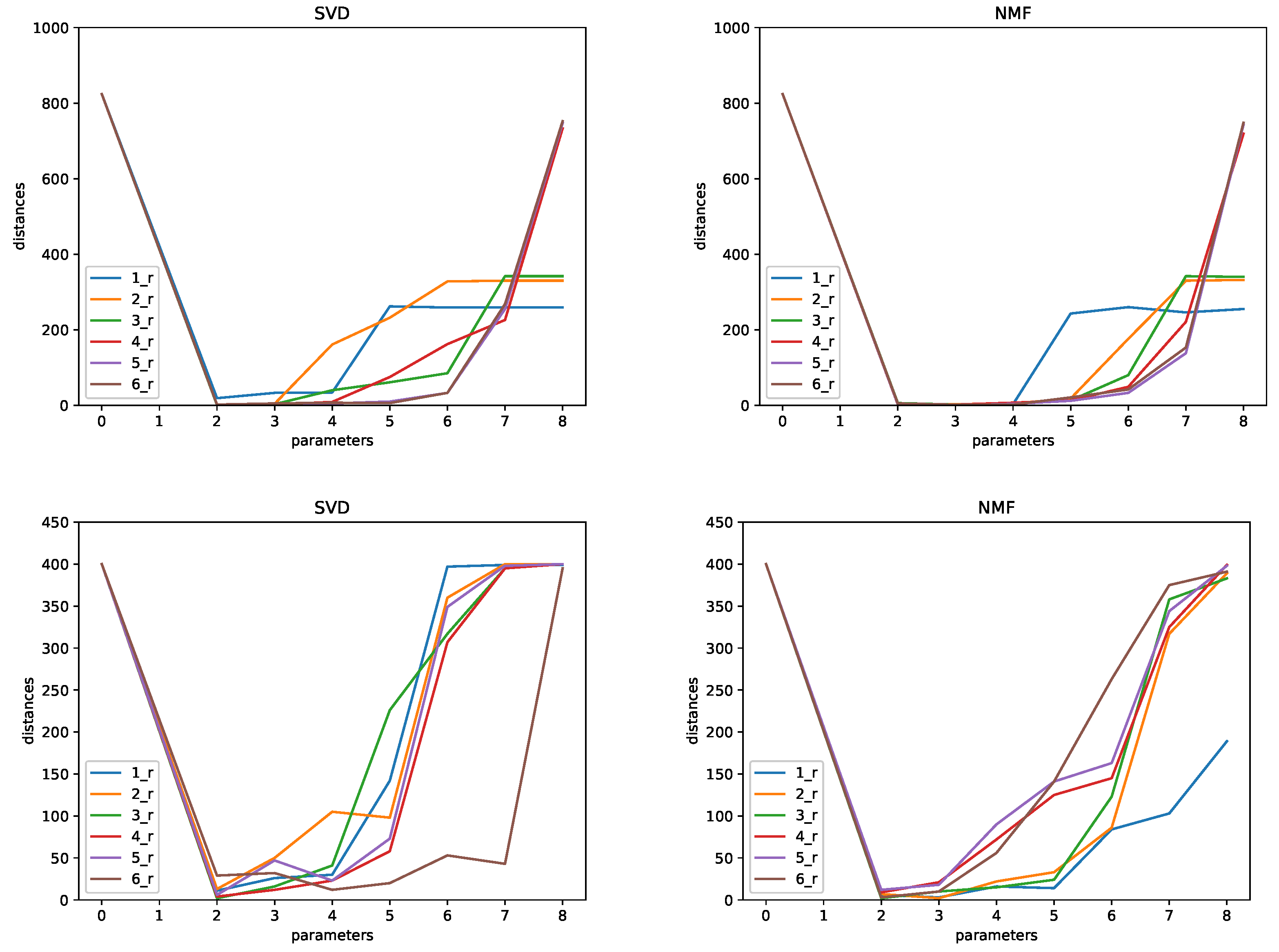
Figure 2 represents the number of correct reidentifications for SVD and NMF-based protection. We can see that there is a drop in the number of reidentifications in this case as well. This drop is not so fast as it is for microaggregation. The figures also show that using more attributes for integration does not mean that the database integration is better. In the case of the Concrete data set, observe that for SVD, one and two attributes lead to better reidentification levels than more attributes (for a number of singular values between three and six). The same pattern appears in the Tarragona data set, and, to some extent, also for NMF-based protection. In contrast, the experiments show that even when we have a low number of correct reidentifications, the machine learning model produced from the integrated database can have similar performance to the one obtained with the original database. We have these results for a significant number of protection levels.

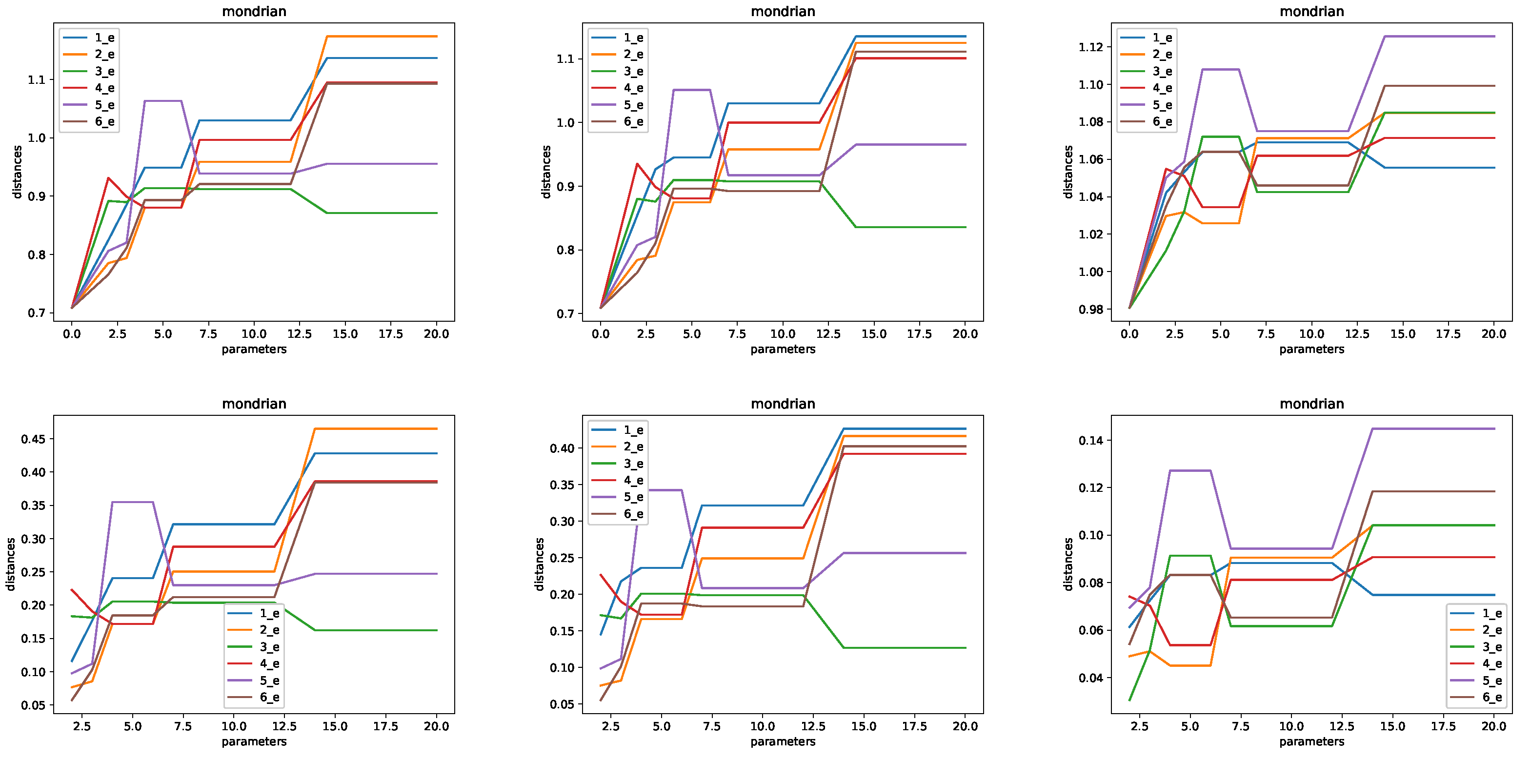
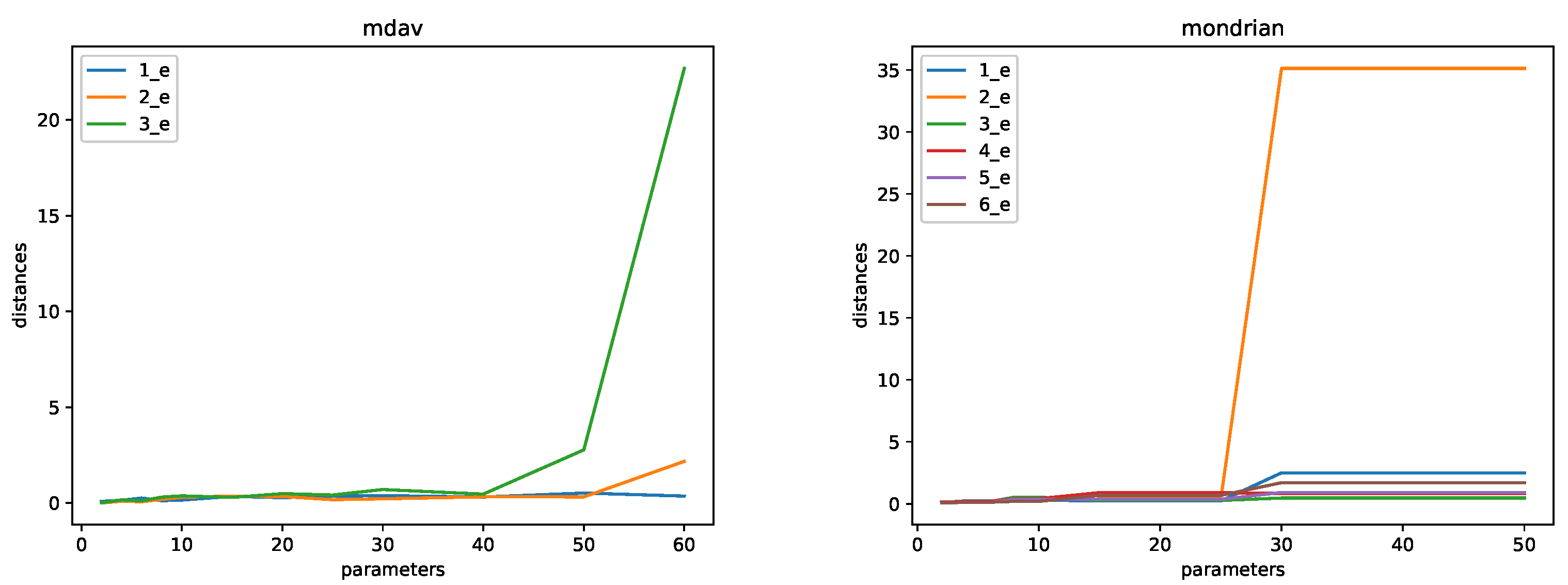
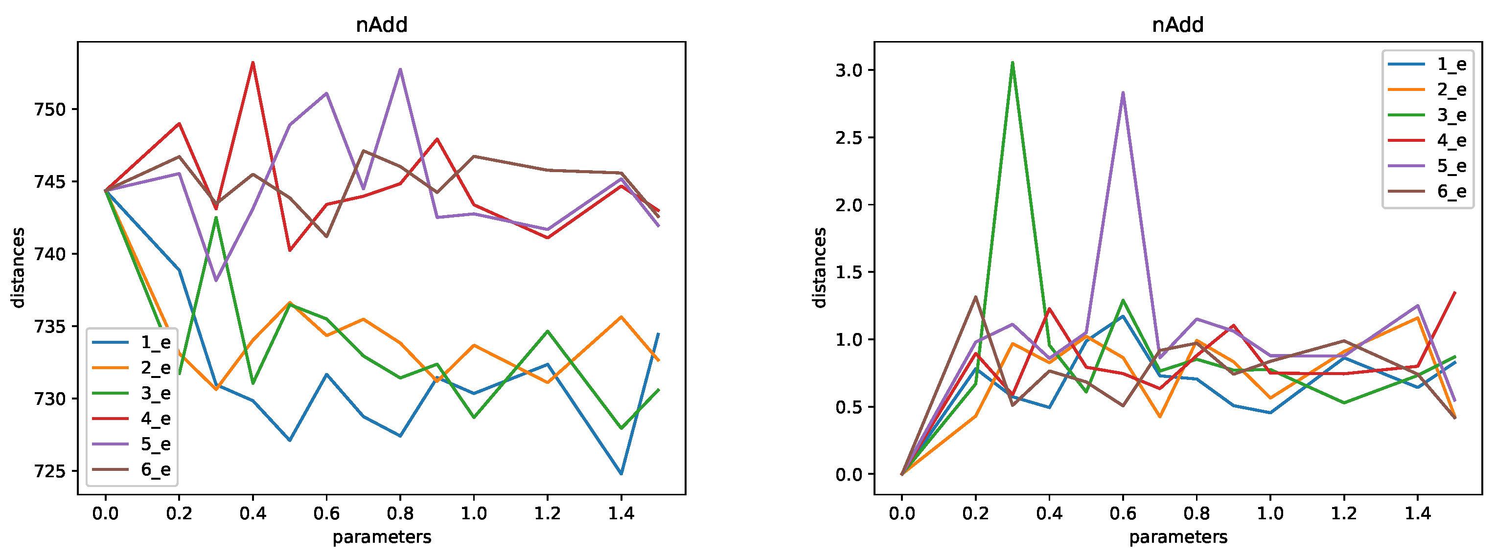
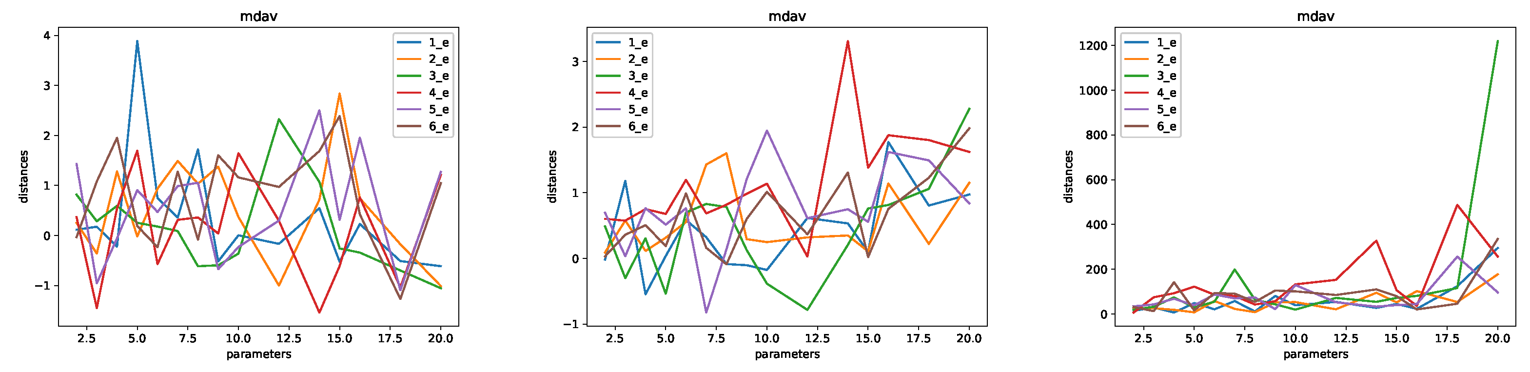
Figure 3 top displays the error obtained for machine learning models extracted from the Concrete data set when these data are protected using Mondrian. In the figures, we have a value of k up to 20, which accounts for significant protection. Note that in the experiments, we use a training set of 824 records, which means that for $k=20$, the k-anonymous file has only 824/20 = 41 different records. Figure 3 bottom shows the difference between the error when we apply the masking method and the error when we do not apply the masking method (i.e., the mean error of the model trained with the original data set). Naturally, larger values of k will result in more distortion of the protected file (fewer different records) and produce a protected database that has low accuracy. In particular, for k equal to or larger than 50 the error becomes extremely large. To illustrate this latter case, we provide in Figure 4 the error for larger values of k. Results are also given for the Concrete database protected using both MDAV (left) and Mondrian (right). In this case, the results correspond to those obtained using a linear regression model. The figures provide the results of different numbers of common attributes.

Figure 3 shows that the error is about 1.1 with significant protection ($k=20$ for microaggregation using MDAV). For comparison and analysis, note that the range between the maximum and minimum values of the output variable in the training set of this figure (Concrete data set) is 80.27, and therefore, a maximum error of 1.5 represents the 1.8% of the prediction output, and a maximum error of 1.0 represents the 1.2% of the prediction output. For $k>60$, the error becomes significantly large. As we have explained above, Figure 4 shows the results for MDAV and Mondrian with values of k up to $k=50$ and $k=60$. Larger values of k produce results with still larger errors. In the case of the Tarragona data set, we show that the range of outputs for the training set is 920,992.0, and then an error of 840 represents 0.91 % of the prediction output. The results of SGD are not displayed; this regression algorithm behaves very badly returning large errors.

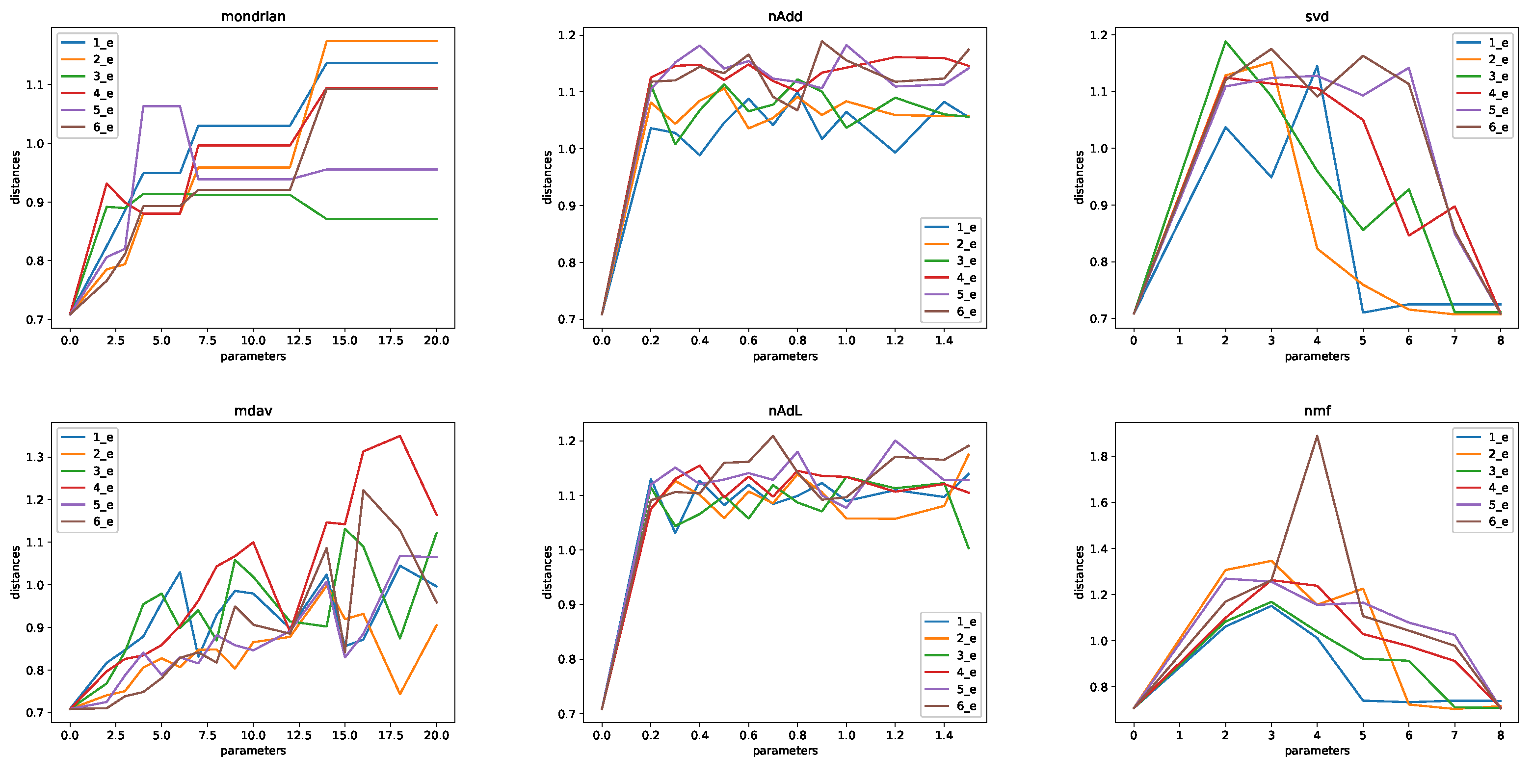
Figure 5 provides similar results (to Figure 3) for linear regression for different masking methods, and different parameters for the same database, the Concrete data set. Errors in the range [0, 2] are shown.

Figure 6 represents the mean and variance for ten executions of the error of the model when data are protected using noise addition. The results correspond to those of the Tarragona data set. Here, the 10 executions are computed on the same training set, but masking noise is applied independently in the 10 runs. A noise parameter equal to zero means no protection. Therefore, for the parameter equal to zero, the 10 executions produce the same model. That is why the standard deviation is zero. This is not the case for non-zero noise. We can see that other parameters have similar variances in the error.

In most of the results described in this work, we have not considered multiple partitions of a database into different training and testing data sets, and the effects of this process. This was considered for two masking methods (microaggregation and rank swapping, using five and ten executions) in our previous work [9], and for microaggregation (using 20 executions) for the CASC data set in Figure 7. We have not considered here multiple executions for all the experiments with all the parameterizations, as this is computationally costly, and we preferred to consider instead more masking methods and more parameters. The results reported here using single executions are consistent with those with multiple executions (in both our previous work and in Figure 7).

5. Conclusions and Future Work

This paper investigated how data masking methods impact the performance of data integration and of machine-learning-based data-driven models. The experimental results show that most of the masking methods we implemented provide good protection even when two individually masked databases are integrated. As the protection increases, the performance of data-driven models decreases. A trade-off of protection and data utility can be achieved through parameterization. A limitation of this study, and of most studies on the effects of masking methods, is that the level of protection depends on both the concrete database and the user requirements. That is, there is no universal solution. In any case, a take-away message of our research is that we can protect data so that correct database integration is avoided while data-driven models can be built successfully, to a certain extent, from the integrated data.

Based on the explorations in this work, there will be several directions for future research. Firstly, in data integration, we can also consider the impact of reidentification from the point of view of the importance of common attributes, in addition to the number of common attributes. Secondly, more fine-tuning of machine learning algorithms can be conducted for better data utility, given the same protection level. Third, we have considered supervised machine learning for numerical data. Extensions for non-numerical (e.g., categorical) data and for unsupervised machine learning (e.g., clustering) are also of relevance. Another line of work is to consider over-representation of individuals [31] and other biases, such as temporal bias [32] and spatial bias [33], applied to the data and see if they affect the results; for example, whether over-representation of some types of users affects the quality of database integration. Finally, our focus was on numerical data. The extension of this work to masking methods for non-numerical data, as well as to protection by means of synthetic data, is another research direction.

References

- Cavoukian, A. Privacy by Design. The 7 Foundational Principles in Privacy by Design. Strong Privacy Protection—Now, and Well Into the Future. 2011. Available online: https://www.ipc.on.ca/wp-content/uploads/Resources/7foundationalprinciples.pdf (accessed on 5 February 2023).
- Duncan, G.T.; Elliot, M.; Salazar, J.J. Statistical Confidentiality; Springer: Berlin/Heidelberg, Germany, 2011. [Google Scholar]
- Hundepool, A.; Domingo-Ferrer, J.; Franconi, L.; Giessing, S.; Nordholt, E.S.; Spicer, K.; de Wolf, P.-P. Statistical Disclosure Control; Wiley: Hoboken, NJ, USA, 2012. [Google Scholar]
- Torra, V. A Guide to Data Privacy; Springer: Berlin/Heidelberg, Germany, 2022. [Google Scholar]
- Herranz, J.; Matwin, S.; Nin, J.; Torra, V. Classifying data from protected statistical datasets. Comput. Secur. 2010, 29, 875–890. [Google Scholar] [CrossRef] [Green Version]
- Mitra, R.; Blanchard, S.; Dove, I.; Tudor, C.; Spicer, K. Confidentiality challenges in releasing longitudinally linked data. Trans. Data Priv. 2020, 13, 151–170. [Google Scholar]
- Wang, H.; He, J.; Zhu, N. Improving Data Utilization of K-anonymity through Clustering Optimization. Trans. Data Priv. 2022, 15, 177–192. [Google Scholar]
- Liu, F. Statistical Properties of Sanitized Results from Differentially Private Laplace Mechanism with Univariate Bounding Constraints. Trans. Data Priv. 2019, 12, 169–195. [Google Scholar]
- Jiang, L.; Torra, V. On the Effects of Data Protection on Multi-database Data-Driven Models. In Integrated Uncertainty in Knowledge Modelling and Decision Making, Proceedings of the 9th International Symposium, IUKM 2022, Ishikawa, Japan, 18–19 March 2022; Springer: Cham, Switzerland, 2022; pp. 226–238. [Google Scholar]
- De Capitani di Vimercati, S.; Foresti, S.; Livraga, G.; Samarati, P. Data Privacy: Definitions and Techniques. Int. J. Unc. Fuzz. Knowl. Based Syst. 2012, 20, 793–817. [Google Scholar] [CrossRef] [Green Version]
- Samarati, P. Protecting Respondents’ Identities in Microdata Release. IEEE Trans. Knowl. Data Eng. 2001, 13, 1010–1027. [Google Scholar] [CrossRef] [Green Version]
- Samarati, P.; Sweeney, L. Protecting privacy when disclosing information: k-anonymity and its enforcement through generalization and suppression. SRI Intl. Tech. Rep. 1998. Available online: https://dataprivacylab.org/dataprivacy/projects/kanonymity/paper3.pdf (accessed on 5 February 2023).
- Dwork, C. Differential privacy. In Automata, Languages and Programming, Proceedings of the 33rd International Colloquium, ICALP 2006, Venice, Italy, 10–14 July 2006; Springer: Berlin, Germany, 2006; Volume 4052, pp. 1–12. [Google Scholar]
- Dwork, C. Differential privacy: A survey of results. In Theory and Applications of Models of Computation, Proceedings of the 5th International Conference, TAMC 2008, Xi’an, China, 25–29 April 2008; Springer: Berlin, Germany, 2008; Volume 4978, pp. 1–19. [Google Scholar]
- Evfimievski, A.; Gehrke, J.; Srikant, R. Limiting privacy breaches in privacy preserving data mining. In Proceedings of the Twenty-Second ACM SIGMOD-SIGACT-SIGART Symposium on Principles of Database Systems, San Diego, CA, USA, 9–12 June 2003. [Google Scholar]
- Winkler, W.E. Re-identification methods for masked microdata. In Privacy in Statistical Databases, Proceedings of the CASC Project International Workshop, PSD 2004, Barcelona, Spain, 9–11 June 2004; Springer: Berlin, Germany, 2004; Volume 3050, pp. 216–230. [Google Scholar]
- Drechsler, J. Synthetic Datasets for Statistical Disclosure Control: Theory and Implementation; Springer: Berlin/Heidelberg, Germany, 2011. [Google Scholar]
- Christen, P.; Ranbaduge, T.; Schnell, R. Linking Sensitive Data: Methods and Techniques for Practical Privacy-Preserving Information Sharing; Springer: Berlin/Heidelberg, Germany, 2020. [Google Scholar]
- Herzog, T.N.; Scheuren, F.J.; Winkler, W.E. Data Quality and Record Linkage Techniques; Springer: Berlin/Heidelberg, Germany, 2007. [Google Scholar]
- Sakuma, J.; Osame, T. Recommendation based on k-anonymized ratings. Trans. Data Priv. 2017, 11, 47–60. [Google Scholar]
- Aggarwal, C.C.; Yu, P.S. A Condensation Approach to Privacy Preserving Data Mining. In Advances in Database Technology—EDBT 2004, Proceedings of the 9th International Conference on Extending Database Technology, Heraklion, Crete, Greece, 14–18 March 2004; Springer: Berlin/Heidelberg, Germany, 2004; pp. 183–199. [Google Scholar]
- Oganian, A.; Domingo-Ferrer, J. On the Complexity of Optimal Microaggregation for Statistical Disclosure Control. Stat. United Nations Econ. Comm. Eur. 2000, 18, 345–354. [Google Scholar] [CrossRef]
- Domingo-Ferrer, J.; Mateo-Sanz, J.M. Practical data-oriented microaggregation for statistical disclosure control. IEEE Trans. Knowl. Data Eng. 2002, 14, 189–201. [Google Scholar] [CrossRef] [PubMed] [Green Version]
- Domingo-Ferrer, J.; Martinez-Balleste, A.; Mateo-Sanz, J.M.; Sebe, F. Efficient Multivariate Data-Oriented Microaggregation. Int. J. Very Large Databases 2006, 15, 355–369. [Google Scholar] [CrossRef]
- LeFevre, K.; DeWitt, D.J.; Ramakrishnan, R. Multidimensional k-Anonymity; Technical Report 1521; University of Wisconsin: Madison, WI, USA, 2005; Available online: https://minds.wisconsin.edu/bitstream/handle/1793/60428/TR1521.pdf?sequence=1 (accessed on 5 February 2023).
- Bozorgpanah, A.; Torra, V.; Aliahmadipour, L. Privacy and explainability: The effects of data protection on Shapley values. Technologies 2022, 10, 125. [Google Scholar] [CrossRef]
- Code Python. Available online: www.mdai.cat/code (accessed on 5 February 2023).
- Templ, M. Statistical Disclosure Control for Microdata Using the R-Package sdcMicro. Trans. Data Priv. 2008, 1, 67–85. [Google Scholar]
- Yeh, I.-C. Modeling of strength of high performance concrete using artificial neural networks. Cem. Concr. Res. 1998, 28, 1797–1808. [Google Scholar] [CrossRef]
- Yeh, I.-C. Analysis of strength of concrete using design of experiments and neural networks. J. Mater. Civ. Eng. 2006, 18, 597–604. [Google Scholar] [CrossRef]
- Wojcik, S.; Adam, H. Sizing up Twitter users. Pew Res. Cent. 2019, 24, 1–23. [Google Scholar]
- Padilla, J.J.; Kavak, H.; Lynch, C.J.; Gore, R.J.; Diallo, S.Y. Temporal and spatiotemporal investigation of tourist attraction visit sentiment on Twitter. PLoS ONE 2018, 13, e0198857. [Google Scholar] [CrossRef] [PubMed] [Green Version]
- Gore, R.J.; Diallo, S.; Padilla, J. You are what you tweet: Connecting the geographic variation in America’s obesity rate to twitter content. PLoS ONE 2015, 10, e0133505. [Google Scholar] [CrossRef] [PubMed] [Green Version]
Figure 1.
Number of correct links for the Concrete data set (top) and the Tarragona data set (bottom) when data are protected using MDAV (top left), Mondrian (top right), noise addition using Gaussian distribution (bottom left), and noise addition using Laplacian distribution (bottom right). Each figure includes curves for different numbers of common attributes (from 1 to 6).
Figure 2.
Number of correct links for the Concrete data set (top) and the Tarragona data set (bottom). Data are protected using SVD and NMF-based protection. The number of correct links decreases when protection is increased (i.e., singular values in SVD and components in NMF). Different curves correspond to different numbers of attributes in the reidentification.
Figure 3.
Output model error (top) for the Concrete data set when data are protected using Mondrian. Output model error difference (bottom) for the Concrete data set when data are protected using Mondrian and when data are not protected. Three different models are considered: linear regression (left), kernel ridge (middle), and support vector regression (right). Figures represent different protection levels and different numbers of attributes in the database integration process.
Figure 4.
Output model error for the Concrete data set when data are protected using MDAV (left) and Mondrian (right). Figures represent different protection levels and different numbers of attributes in the database integration process. A larger discrepancy is shown in the figure for 3 common attributes in MDAV and for 2 common attributes in Mondrian.
Figure 5.
Output model error for the Concrete data set when data are protected using microaggregation (left—MDAV and Mondrian), noise addition (middle—Gaussian noise and Laplacian noise), and dimensionality reduction (right—NMF and SVD-based). Figures represent different protection levels and different numbers of attributes in the database integration process. Figures correspond to linear regression.
Figure 6.
Mean output model error (left) and its variance (right), for 10 executions, for the Tarragona data set when data are protected using noise addition. The machine learning model considered is linear regression. Figures represent different protection levels and different numbers of attributes in the database integration process.
Figure 7.
Results for the CASC data set masked using MDAV and for linear regression, comparison for . Result of a single execution (left), mean results of 20 executions (middle), and variance of 20 executions (right).
Disclaimer/Publisher’s Note: The statements, opinions and data contained in all publications are solely those of the individual author(s) and contributor(s) and not of MDPI and/or the editor(s). MDPI and/or the editor(s) disclaim responsibility for any injury to people or property resulting from any ideas, methods, instructions or products referred to in the content. |
© 2023 by the authors. Licensee MDPI, Basel, Switzerland. This article is an open access article distributed under the terms and conditions of the Creative Commons Attribution (CC BY) license (https://creativecommons.org/licenses/by/4.0/).
Share and Cite
MDPI and ACS Style
Jiang, L.; Torra, V. Data Protection and Multi-Database Data-Driven Models. Future Internet 2023, 15, 93. https://doi.org/10.3390/fi15030093
AMA Style
Jiang L, Torra V. Data Protection and Multi-Database Data-Driven Models. Future Internet. 2023; 15(3):93. https://doi.org/10.3390/fi15030093
Chicago/Turabian StyleJiang, Lili, and Vicenç Torra. 2023. "Data Protection and Multi-Database Data-Driven Models" Future Internet 15, no. 3: 93. https://doi.org/10.3390/fi15030093
Note that from the first issue of 2016, this journal uses article numbers instead of page numbers. See further details here.