
Artificial-Intelligence-Based Charger Deployment in Wireless Rechargeable Sensor Networks


1
Department of Computer Science and Information Engineering, National Ilan University, Yilan 260, Taiwan
2
Department of Computer Science and Information Engineering, National Dong Hwa University, Hualien 974, Taiwan
3
Department of Computer Science and Information Engineering, National Cheng Kung University, Tainan 701, Taiwan
4
Department of Electrical Engineering, National Dong Hwa University, Hualien 974, Taiwan
5
Institute of Computer Science and Innovation, UCSI University, Kuala Lumpur 5600, Malaysia
*
Author to whom correspondence should be addressed.
Future Internet 2023, 15(3), 117; https://doi.org/10.3390/fi15030117
Submission received: 20 December 2022
/
Revised: 8 March 2023
/
Accepted: 13 March 2023
/
Published: 22 March 2023
(This article belongs to the Special Issue Distributing Computing in the Internet of Things: Cloud, Fog and Edge Computing)
Abstract
:To extend a network’s lifetime, wireless rechargeable sensor networks are promising solutions. Chargers can be deployed to replenish energy for the sensors. However, deployment cost will increase when the number of chargers increases. Many metrics may affect the final policy for charger deployment, such as distance, the power requirement of the sensors and transmission radius, which makes the charger deployment problem very complex and difficult to solve. In this paper, we propose an efficient method for determining the field of interest (FoI) in which to find suitable candidate positions of chargers with lower computational costs. In addition, we designed four metaheuristic algorithms to address the local optima problem. Since we know that metaheuristic algorithms always require more computational costs for escaping local optima, we designed a new framework to reduce the searching space effectively. The simulation results show that the proposed method can achieve the best price–performance ratio.
1. Introduction
Recently, wireless sensor networks (WSNs) [1,2,3] have been among the most widely used techniques due to people wanting to easily collect more and more information about everything. For example, people want take care of their elderly family and enhance the quality of their family life. They use various sensors to collect heartbeat, blood pressure and sleep quality of the elderly or ill [4,5], so that family members can instantly handle any status. As another example, a wrong command may cause soldiers’ deaths in a war, so the army needs to use WSNs to get useful data to ensure correct commands. Furthermore, some dangerous environments may need to be investigated, such as volcanoes and underwater environments [6,7,8]. In these cases, sensors can serve as the competent technology to sense anything in a variety of harsh environments. Obviously, WSNs are gradually affecting our lives more and more.
However, WSNs still have some intrinsic problems. A WSN is composed of wireless sensors and some relay nodes. Each sensor node will sense various kinds of information and then transfer it to the relay nodes. All of these actions will consume power, but a sensor’s power is limited by battery capacity so that its power will be exhausted. Many sensors collect multimedia data, and their power consumption will be more obvious. Note that these sensors may be placed in the dangerous places we just mentioned, so that we cannot immediately replace the batteries; therefore, the WSN will be paralyzed if the relay node dies. In view of this, researchers have proposed some methods to solve the network lifetime problem [9,10,11,12]. Some scholars think that all of the sensors should not work at the same time because it will cause power to be wasted unnecessarily. Scheduling sensor working time can make efficient use of the power of sensors. However, the lifetime of the WSN still depends on the upper bound of a battery’s capacity 12; this is a fact which cannot be changed.
In order to solve the power problem, the development of wireless charging technology has been proposed for wireless rechargeable sensor networks (WRSNs) [13,14,15,16]. A WRSN is composed of charger, sensor and relay node; the charger is the main power source in such an environment. Each WRSN has its own suitable environment so that the user is able to choose specialized charging equipment according to his requirements. Of course, different charger equipment has different wireless charging methods. For example, wireless charging technology of mobile phone uses electromagnetic induction.
WRSNs can be roughly divided into two types: those that operate in indoor environments, and those that operate in outdoor environments. The deployment strategy of the chargers needs to consider various impacts from those different environments. Most studies discuss outdoor scenarios; too few studies consider indoor scenarios. Actually, wireless sensor networks are very helpful indoors as well [17,18]; for example, they can help factories control production for better quality and provide disaster prevention and relief. Life will become more convenient if sensors never run out of power. This is one of the main reasons why the wireless rechargeable sensor network is increasingly popular. In this paper, the deployment scenario is the indoor environment; it entails a complex problem because the charger deployment strategy will be affected by the sensors’ positions, RF interference and the charger’s efficiency, since those metrics have very frequent trade-off relationships. We have to balance each factor and then make sure the resultant deployment strategy can provide more charging efficiency. In previous work, we proposed the moveable-charger-based algorithm (MCBA) [19] to achieve a good charger deployment strategy. First, find the candidate nodes for charger deployment through mapping. Calculate the number of sensors that each candidate node can cover. Then, select candidate nodes in order from large to small by sorting until all sensors are covered. However, MCBA still has some defects, such as the MCBA being a greedy-based algorithm, so it has more of an opportunity to fall into the local optimum. The charger deployment has been proven to be an NP-hard problem. Since charger deployment has been proven to be an NP-hard problem, it is inefficient to solve this problem by using brute-force algorithms [17]. In order to solve this problem and to reduce deployment costs as much as possible to achieve optimization, we used a metaheuristic algorithm to design a charger-deployment algorithm.
Although metaheuristic algorithms are potential methods to find better solutions [20,21], the optimal solution can only be found through a large number of iterations, thereby costing more computational time to converge. Therefore, excluding non-essential solutions is a necessary step. This paper makes two major contributions: (1) we used four metaheuristic algorithms to design the strategy for charger deployment; (2) we proposed a layoff algorithm to improve these metaheuristic algorithms and analyzed each algorithm to determine in which scenario it is suitable for the application.
The sections of this study are as follows. In Section 2, the background knowledge of wireless rechargeable sensor networks and related research papers are briefly described, analyzed and discussed. In Section 3, problem definition is introduced. The proposed schemes are presented in Section 4. The simulation results are shown in Section 5. Finally, the conclusions are discussed and future developments are proposed.
2. Related Works
To clearly present this paper, we introduce the backgrounds of WRSN, previous works and some metaheuristic algorithm as follows.
2.1. Wireless Rechargeable Sensor Network
Wireless charging technologies can be divided into two categories according to their power sources. The first category involves using the power of nature, such as wind power and solar power. The power of nature will be changed to alternating current to power equipment. However, it will be limited in the environment; the sensor will die if the natural power is gone because it is not always sunny or windy. The second category involves power which is less influenced by the environment. The common charging techniques are as follows: (1) magnetic induction [22], (2) magnetic resonance [23], (3) laser light sensor [24] and (4) micro-wave conversion [25].
2.2. Wireless Charging Planning
Some scholars mapped the charging problem as a Hamilton cycle and let the whole environment be divided into multiple clusters. They also proposed a greedy-based 26 algorithm to find a shortest path for charging. However, this method did not consider that some sensors have too little energy so that they will run out of energy before charging vehicles arrive [26]. In [27], the authors took Washington as an example. They tried to detect the number of pedestrians from infrared images and then figured out which area of pedestrians is the most intensive. The major goal of this work was to improve the survival rate of terminal devices. However, statistics-based methods usually do not have good environmental adaptability. In [28], the authors used unmanned aerial vehicles (UAVs) for charging. They can be used in the extremely rough terrain which cannot be traversed by self-propelled vehicles. The authors also divided the sensors into multiple clusters. The data of sensors were transmitted when the UAV was arriving for charging. Their proposed one-side matching algorithm considers the remaining power and distance of UAV flight to calculate the optimal charge-priority order. In addition, some scholars considered the collision avoidance [29], minimum number of disjoint shortest trees [30] and multiple self-propelled vehicles [31] to design a better charging plan. Most works adopted intermittent charging. This means that the charging process only begins when the self-propelled vehicle has arrived, and then it will stay in there until the termination condition is met. However, sensors will sense current as long as the self-propelled vehicle passes by them. In [32], the authors proposed a real-time charging method to extend network lifetime. The authors proposed a spatial-temporal discretization method in which each time block is independently assigned based on travel speed and the distance from the sensors. In other words, this method can optimize where to go to charge the sensors. For the indoor scenario, the authors of [19] proposed a greedy-based method to quickly deploy chargers. In [33], the authors adopted the concept of a center of gravity to find the best charging position and proposed a charging-schedule algorithm to increase the remaining-use durations of sensor nodes. In [34], the authors proposed a particle swarm charger-deployment algorithm that utilizes the local optimal result and the global optimal result to adjust locations and antenna orientations of chargers.
2.3. Movable-Charger-Based Algorithm
Most studies on WRSNs involve an outdoor scenario planning the path for charging a car or airplane, so it is necessary to further charging technology, including the indoor scenario. In our previous work, we proposed the minimum-charging-based algorithm (MCBA) to deploy charging in an indoor scenario and a novel means of reducing the deployment cost. They have the advantages of centralized power and a large charging area.
The MCBA step can be divided into two parts. The first is finding a candidate charger. The IoT is located by aGPS. We then map the transmission range of the sensor nodes to the ceiling. This means that the sensor will be charged if the charger is deployed there. The second is finding the optimal position where the charger will be finally deployed. The increased overlapping area means that the charger can cover more sensors. We used this point to find the better solution.
3. Problem Definition
The WRSN scenarios can be simply divided into indoor and outdoor scenarios. Different environments will affect the problem definition and the code of the solutions. In this paper, we focus on the deployment problem in an indoor scenario. The network model and wireless charger model will be presented in the next part.
3.1. Network Model
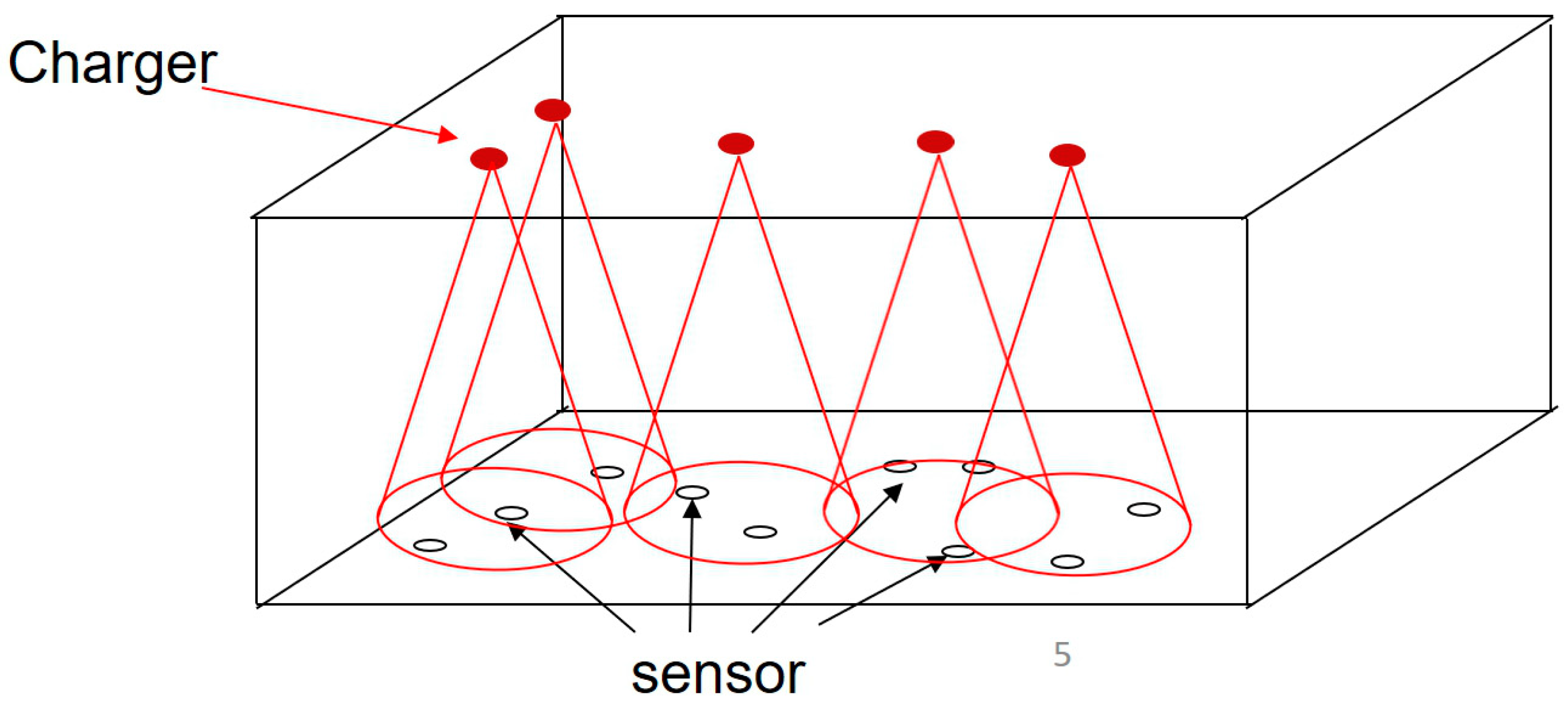
A wireless rechargeable sensor network model is as follows, where is a subset of candidate chargers in the network, is a set of subset of sensor nodes in the network and is a subset of the final positions of deployed chargers. Sensor nodes are deployed randomly in 3-dimension space. Each sensor node can receive power from the chargers. To reduce the impacts of interference and obstacles, the chargers were deployed on the ceiling that is shown in Figure 1. The chargers emitted a radio wave down to cover the sensors. Each charger has its own effective charging distance (ECD) so that each sensor can enjoy better charging efficiency when the distance from sensor to charger is closer, and vice versa. To ensure that each sensor can be charged effectively, we assume that the height of the indoor scenario must be less than the ECD, which is defined in Equation (2). In this paper, we followed the method of positioning the candidate charger from our previous method, MCBA.
3.2. Wireless Charging Model
The most important deployment problem is that the power consumption of each sensor node differs because each sensor has its own sensing function and power consumption. Therefore, we must calculate the received power of each sensor:
where represents that the sensor’s power received from the charger; represents power transferred from the charger to the sensor; is a value of antenna gains of the chargers; represents a value of antenna gains of sensor nodes; is a value of rectifier efficiency; is polarization loss; is the wavelength of RF; is a unique adjustable parameter in an indoor environment. To ensure each sensor can be charged, the first step is to find the amount of power which the most power-hungry sensor needs. If the provided power can meet the requirements of the most power-hungry sensor, all of the sensors can receive enough power in this scenario. In view of this, we further define the ECD, as shown in Equation (2)
where R is ECD; is the maximum power consumption of all sensors; N is the number of chargers needed for the most power-hungry sensor. We assume ; it represents that the most power-hungry sensor will run out of power received from the chargers. In other words, all of sensors will receive enough power when the distance of sensor to charger is between R. According this assumption, R is also equal to . We can deduce Equation (1) by Equation (2).
We assume that all of chargers will provide the same power to have better fairness. The charging efficiency is better when the effective charging distance is less than R, and vice versa.
3.3. Linear Programing Model
In this paper, we follow the method of finding the position of a candidate charger by our previously proposed method, MCBA. In order to decrease the deployment cost and reduce the chance of falling into the local optimum, we use a metaheuristic algorithm to solve this problem. According to the above-mentioned expected goal, we define a linear programing model for this problem:
The main goal of this paper is to minimize the number of chargers, , and make sure that each sensor can continue working. A lot of chargers will lead to a higher deployment cost. Conversely, fewer chargers will lead the power of sensor nodes to become exhausted more quickly. Therefore, the most important thing is to balance these two metrics to make sure that sensor nodes can continue working. We defined some restrictions to make this paper closer to a real scenario. The first restriction represents that sensor nodes’ total collected power must be larger or equal to the power consumption. According to the energy conservation law, the chargers’ power needs to be greater than the power received by the sensor nodes because power will be lost during the process of power transfer, as described in the second restriction. To guarantee that the sensor nodes will be charged exactly, the third restriction is to restrict the efficient charging distance. This means that the distance between the charger and sensor must less than E. For deployment results, the energy efficiency must be greater than zero as the fourth restriction. Energy efficiency means the sum of the energy received by all sensors divided by the number of chargers.
4. Proposed Scheme
The subset of a candidate charger was calculated by our previous work. How to find the best solution from among a lot of candidate chargers is an NP-hard problem. The exhaustion method is a complete solution for optimization finding, but it will entail more computational costs and time. Therefore, we used the concept of metaheuristic algorithms to design our method. Although a metaheuristic algorithm cannot guarantee that the best solution can always be found, it still finds an acceptable solution in time. In order to speed up the time to find the best solution, we use the simulated annealing algorithm (SA), tabu search algorithm (TS), genetic algorithm (GA) and ant colony optimization (ACO); and we propose a layoff algorithm (LA) to enhance it in this study.
4.1. Metaheuristic Algorithm
Different coding methods can affect the final results. In order to compare all of algorithms fairly, we used the same coding method for them. Each candidate charger position has two statuses. The Boolean value of one represents a charger to be deployed, and vice versa. In order to judge the quality of the solution, we define the fitness function as follows:
4.2. SA-Based Charging Algorithm
The concept of SA is that some worse solutions have the chance to be accepted [35]. In other words, this method can reduce the chance of falling into a local optimum. Thus, we used the SA concept to design a deployment method that is called the SA-based charging algorithm (SABC). With SABC, candidate chargers will be randomly chosen in the beginning. The status of candidate chargers will be changed at every iteration. This means that this method will compare various possibilities for making a decision as to whether or not to deploy the charger according to f(x). The SA predetermined temperature will continue to decrease. When the temperature is still high, it has a high probability of accepting poor solutions. The temperature needs to be lowered because convergence that is too fast will lead to the solution quickly falling into the local optimum. The probability that a poor solution can be accepted declines when the temperature decreases. The reason is simple: the final solution may become a set of low-quality solutions if poor solutions are always accepted in each iteration.
The first step is that SABC creates a number of bits; the values of the bits are represented by 1s or 0s randomly. A value of 1 means that the candidate charger can be deployed in this position, whereas 0 means that the charger is not deployed. We set the experimental group and control group fairly. However, in copying the L neighbor solution, L is a value which can be freely adjusted by the user. The next step is to randomly change the status of bits and calculate f(x). If the solution meets the threshold of acceptance, the experimental group will be replaced; this process is repeated until the termination criterion is met.
In this section, we show the pseudocode of the algorithm. In the first step, we set an initial temperature by the annealing schedule and randomly created an initial solution , as shown in lines 1–2 of Algorithm 1. To compare the quality of solutions, f(x) will be calculated for any just found solution, as shown in line 3. The next step is randomly choosing from each solution and changing the status shown in line 5. Line 6 shows that the original solution and new solution will calculate their f(x). We can replace the original solution if the new solution is better, and the temperature, as shown in lines 7–9, is also adopted. The last step is to update the temperature according to the SA rule. This process is repeated until the termination criterion is met.
| Algorithm 1 SA-based charging algorithm (SABC) |
| SA-Based Charging Algorithm (SABC) |
| Input: Outpus:
|
|
|
|
|
|
|
|
|
4.3. TS-Based Charging Algorithm
The concept of the TS is that the best solution will be recorded in the tabu list [36]. Therefore, the solution will be better than those before each iteration. The tabu list can avoid some solutions which were found repeatedly. In other words, the main principle of TS using the tabu list is to record the best solution of each iteration. However, we can find better solutions via a comparison with all the previous experiences. We used this concept to design the charger deployment algorithm called the TS-based charging algorithm (TSBC). In the beginning of TSBC, candidate chargers are chosen randomly. The deployed status of candidate chargers will be changed in each iteration. The solution can be evaluated by f(x). We can find the current best solution and record it in the tabu list. Note that if the currently found solution is the same as the solution recorded in the tabu list, we cannot accept it, even if it is better. This is like human memory; information will be stored in the memory for a long time. The size of the tabu list will affect the quality of solutions and the computational cost, as too much storage will increase the time spent on checking the TS list, thereby increasing the computational time. With too little storage, past experience cannot be completely recorded. In view of this, the storage of the tabu list should be changed according to environmental factors. This is an important parameter in TS.
The first step creates bits; the value of each bit will be randomly set as 1 or 0. A value of 1 means that the candidate charger is able to deploy in this specified position, and a value of 0 represents that the charger cannot be deployed in this position. To ensure the fairness in comparing algorithms, we set up the experimental group and control group. We copied the L neighbor solution as the experimental group. Then, was chosen randomly, and the status of was reversed. The next step was calculating the f(x) of the solution. If the solution was better than before and was not the same as a solution on the tabu list, the experimental group was replaced; this process was repeated until the termination criterion was met.
In the first step, we randomly create the initial solution and empty the tabu list, as shown in lines 1–2 of Algorithm 2. To compare the quality of the experimental group and control group, f(x), as shown in line 3, is calculated. The next step is to randomly choose , change the status of and compare their f(x), as shown in lines 5–6. We can replace the solution if another one’s f(x) is better and the solution is not the same as a solution on the tabu list, as shown in lines 7–9. The last step is to update the tabu list. If the size of the tabu list is exceeded, we use first-in first-out (FIFO) as the main process to record the next solution. Finally, this algorithm will repeat until the termination criterion is met.
| Algorithm 2 TS-based charging algorithm (TSBC) |
| TS-Based Charging Algorithm |
| Input: Output:
|
|
|
|
|
|
|
|
|
|
4.4. GA-Based Charging Algorithm
The concept of the GA [37,38], as mentioned above, originated from the theory of evolution. The GA-based charging algorithm (GABC) based on this concept was used to design the deployment problem. In this paper, the chromosome represents the solution. The gene represents the candidate position and whether or not it will be deployed. GABC is composed of three steps. The first step is selection. We can choose a better solution according to f(x). This is an important mechanism for convergence. The better solution will be selected, and the worse one will be eliminated. The second step is crossover. Chromosomes can exchange genes with each other. In this way, the solution will be better because the better chromosomes will be chosen in the selection. The third step is mutation. The gene has an opportunity to change the status of genes in each chromosome so that the solution will have the ability to avoid fall into a local optimum through mutation. The GA’s greatest difference from SA and TS is that they are single-solution methods, whereas the GA is a multi-solution method. This means that the GA has a large solution space to expand and find the best solution, although it will require more computational time.
The first step is to create L chromosomes. A difference from SA and TS is that the GA needs different chromosomes to evolve, so genes of the chromosomes have different statuses. In the second step, we need to calculate fitness function f(x). The third step is selection, which can choose a better solution by f(x). The fourth step is crossover. The fifth step is mutation. All of the above steps will repeat until the termination criterion is met.
This part shows the GABC algorithm by its pseudocode. The first step is to randomly create the initial chromosomes whose length is shown in line 1 of Algorithm 3. Note that each status of the gene will be created randomly, ensuring biological diversity. Each chromosome will then calculate the f(x), as shown in line 3. The next step is selection: randomly choosing two chromosomes to compare them with f(x) and then saving the better one, as shown in line 4. The following step is crossover: randomly choosing two chromosomes and then exchanging the genes randomly, as shown in line 5. The next step is mutation: randomly choosing genes to exchange their statuses. For example, a candidate charger will change its status from “to be deployed” to “not to be deployed”, as shown in line 6. This process is repeated until the termination criterion is met so that the best chromosome will be found.
| Algorithm 3 GA-based charging algorithm |
| GA-Based Charging Algorithm |
| Input: Output:
|
|
|
|
|
|
|
|
|
|
4.5. ACO-Based Charging Algorithm
The concept of ACO originated from the behavior of ants seeking food [39]. Ants will follow the pheromone on the road where other ants have walked. The other ants can find the better solution according to the pheromone. We used this concept to design the deployment algorithm that is called the ACO-based charging algorithm (ACOBC). In this method, ants will walk to the position of the candidate charger. If this position is a better solution, the ant pheromone will remain, and vice versa; that is called online updating. At the end of each run, the pheromone will be updated offline regarding the best road in this run. Offline updating is a method by which to follow the best previous experience. The other important factor of ACOBC is overlapping areas. The solution will be better if the overlapping area is small. The directions of ant searches will be decided according to both above-mentioned factors. To make the solution converge, the pheromone will evaporate if ants have not walked there. In the beginning, the direction of ants searching will be decided by the factor of overlapping. As the values of the pheromones are the same, the solution will avoid falling into the local optimum through randomly choosing nodes at the beginning and updating pheromones. Ants will choose the candidate charger according to , which is calculated as follows:
where is the pheromone; is the value of overlapping; and are the values of weights and can be adjusted in different environments. Ants will walk to each position of candidate chargers only once and ensure that the solution will not fall into an infinite loop. At the outset, ACOBC does not choose any candidate charger. Ants will choose the direction of the solution according to . When an ant arrives at a new node, ACOBC will evaluate the deployment status and whether or not to deploy by f(x). The position which ants have arrived at will be recorded on the checklist to ensure that the ants has arrived only once at each position. The position of the candidate charger will be deployed and updated on the online pheromone if the value of f(x) is better than that. If the value of f(x) is worse, the checklist is updated but not the online pheromone, as shown in case 2. The pheromone which ants retained as the best solution will be updated offline in the end. We present the ACOBC algorithm by its pseudocode. The first step initiates the values of and , while setting the solution value as zero and calculating the f(x), as shown in lines 1–3 of Algorithm 4. The number of ants is . Each ant will choose the position by and update the checklist; the f(x) will be calculated at the same time, as shown in lines 7–8. If ants arrived at new positions and the f(x) will be better, pheromone will be added and the online pheromone updated, as shown in lines 9–11. The covered sensor will be recorded in . If the value of is equal to the value of , the ant is finished finding positions in this run. In other words, all the sensors will be covered by the candidate charger shown in lines 12–13. In the end, the best solution is found to update the online pheromones, as shown in lines 16–17.
| Algorithm 4 ACO-based charging algorithm (ACOBC) |
| ACO-based charging algorithm (ACOBC) |
| Input: Output:
|
|
|
|
|
|
|
|
|
|
|
|
|
|
|
|
|
|
|
|
4.6. Layoff Algorithm
Although metaheuristic algorithms can find the better solutions, they still have some defects. For example, they will require a lot of computational time to converge. As metaheuristic algorithms will continue to repeatedly match all of the solutions to find the best solution, this process will waste computation. The solution has a chance of falling into a local optimum when using a metaheuristic algorithm. As the deployment problem is a continuity problem, the candidate chargers which are deployed in the beginning can cover a greater area and have fewer overlapping areas. The coverage area will be smaller when the candidate charger continues to be deployed. This phenomenon will apparently occur when the sensor nodes are increased in number, so we propose using the layoff algorithm (LA) to solve it.
The concept of the LA has two parts. The first part involves removing useless candidate chargers to reduce the computational time. The second part is to ensure that the sensor nodes will be covered in each iteration. According to this concept, not only can the quality of the solution be promised, but it can also ensure that the lost-covered-sensor problem will not happen. We define fitness function as follows:
In the LA, the first step is randomly firing the candidate chargers and updating the CCL. If the CCL complies with the standard, the calculated. If the CCL does not comply with the standard, it will randomly choose new . The next step is to calculate . It can evaluate the quality of the solution.
In the layoff algorithm, all the sensor nodes will be covered in each iteration. The value of can be simplified to 1 to decrease the computational time. All the candidate chargers will be deployed in the beginning. We can lay off the useless positions of candidate chargers in each iteration. Notice that the layoff algorithm is just a screening scheme for the selection and deletion of candidate chargers. It cannot work alone but can be combined with any metaheuristic algorithm. We used pseudocode to represent the layoff algorithm. The first step is to create the initial solution and the CCL, and then calculate the initial fitness function, as shown in lines 1–2 of Algorithm 5. In the next step, the position of the candidate charger is randomly laid off. If the solution is better, will be laid off, and vice versa, shown in lines 4–7 of Algorithm 5. The detailed method of design is presented in the next part.
| Algorithm 5 Layoff algorithm |
| Layoff Algorithm |
| Input: Output:
|
|
|
|
|
|
|
|
|
5. Simulation Results
5.1. Simulation Settings
In this study, we adopted Matlab (Version 7.11, R201b) as the simulation tool. The scenario of our paper was a 30 25 3 indoor environment. The number of sensor nodes was set as 50 to 400, and they were randomly deployed. The effectual charger distance was 5 m. The details of simulation parameters are shown in Table 1.
5.2. Deployment of Chargers
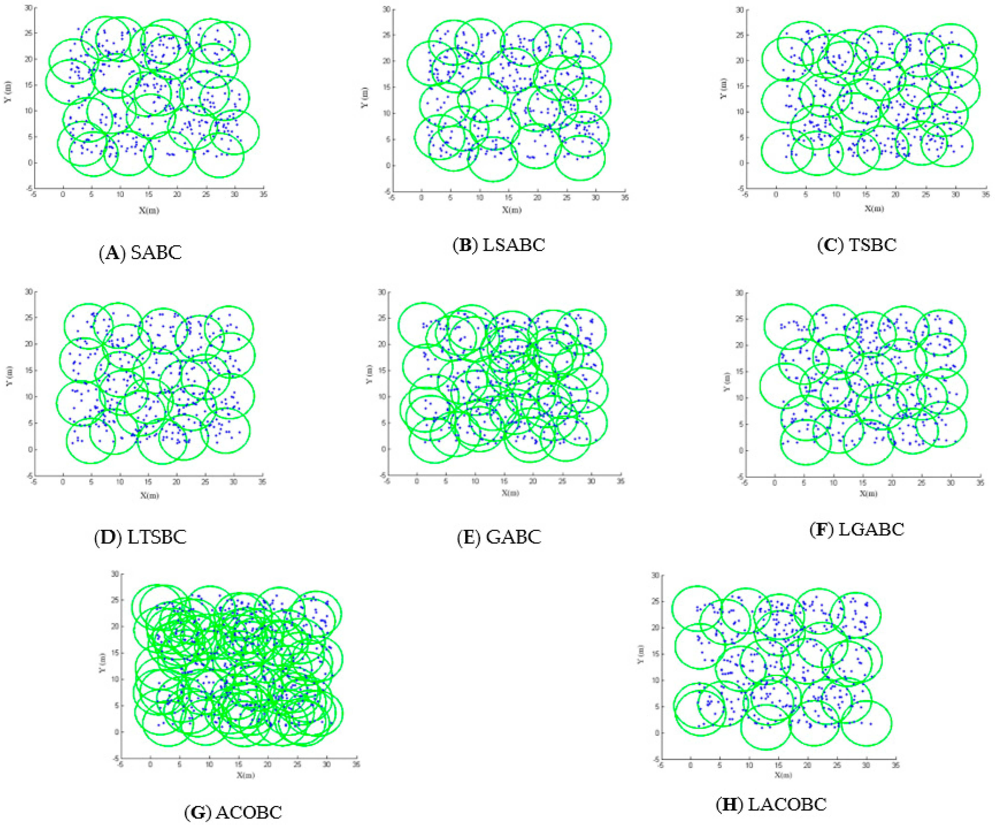
Figure 2A,B show the deployment of SABC and LSABC; the blue points are sensor nodes. Green circles are charger areas. There were 400 sensor nodes randomly deployed. The simulation shows that SABC can cover most of sensor nodes, but the sensor node in the upper left corner is ignored. Conversely, LSABC can cover all of the sensor nodes. This means that SABC still cannot completely avoid falling into a local optimum.
Figure 2C,D show the area covered by TSBC and LTSBC. The sensor nodes in the upper left corner were not covered by TSBC. In other words, TSBC still cannot completely break through the local optimum problem.
Obviously, the GABC cannot choose suitable candidate chargers to cover all the sensor nodes. In Figure 2E, there are many overlapping areas. In other words, many unnecessary candidate chargers are deployed by GABC. The charger which had not been deployed has a chance to be deployed in the mutation of GABC. That is the season why GABC cannot converge, as shown in Figure 2E,F.
The deployment of both ACOBC and LACOBC is shown in Figure 2G,H. The concepts of ACOBC and LACOBC completely differ. Ants will choose the best candidate charger in the ACOBC. In the LACOBC, ants will choose which candidate charger should be laid off. There was a problem when all of sensor nodes were covered: the ant would stop seeking the next node in GABC. In each iteration, the ants could not find all of nodes; this led to a worse solution.
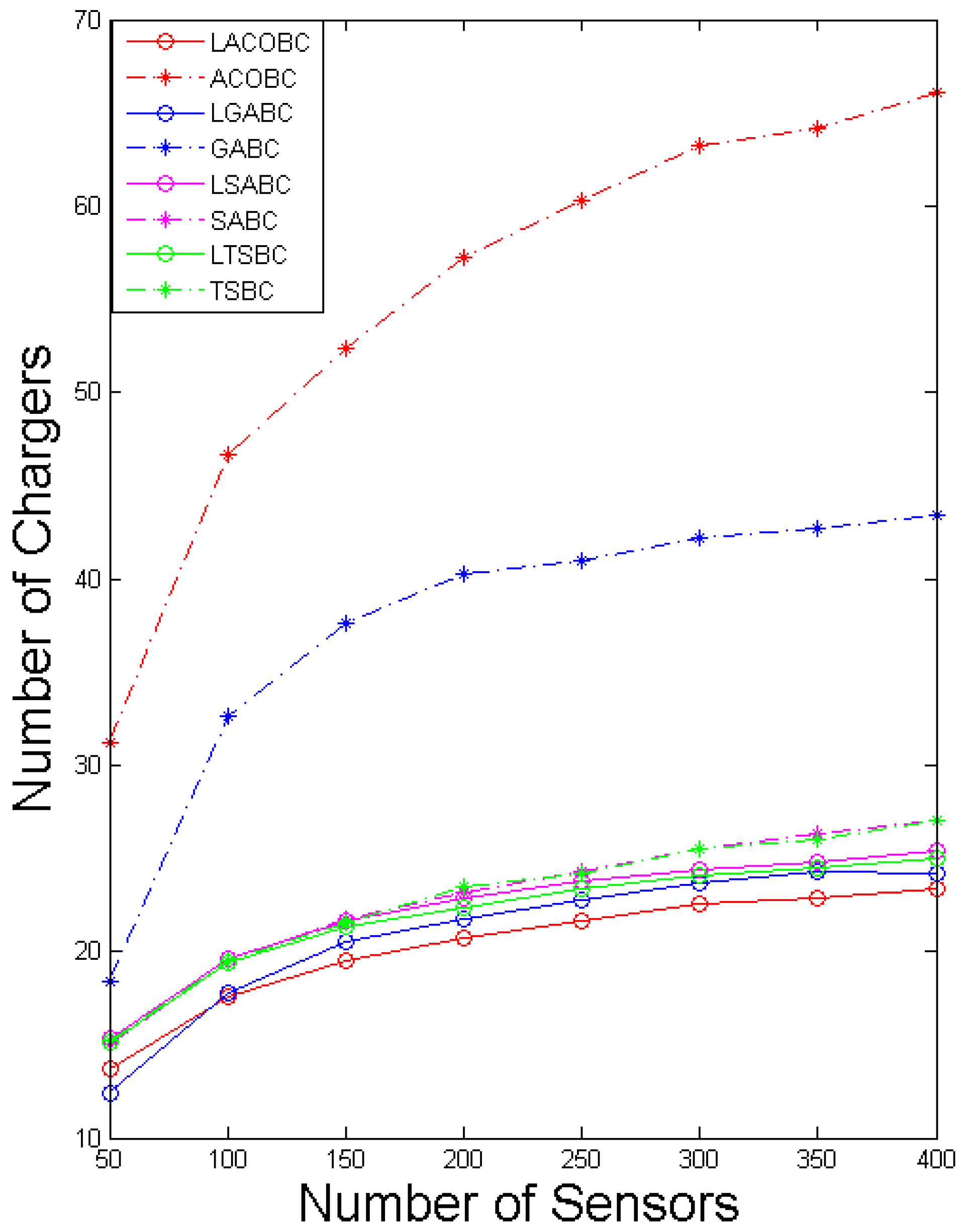
5.3. Comparison of Number of Chargers
In this section, we compare the number of chargers while the number of sensor nodes increased from 50 to 400. The x-axis represents the number of sensors, and the y-axis represents the number of chargers. To ensure objectivity and accuracy, all of the algorithms performed 1000 iterations.
Figure 3 shows a comparison of the number of chargers for SABC and LSABC. In the LSABC, if the number of sensor nodes increases, the curve of LSABC will tend to signify an exponential function. This phenomenon shows that the LSABC can effectively avoid falling into a local optimum. SABC’s deployment cost will increase when the number of sensor nodes increases.
The growth curves of LTSBC and TSBC are like those of LSABC and SABC. According to the coding method of SA and TS, they can be classified as a single solution. The layoff algorithm can help the single solution to have better quality; the benefit will be notable when the number of sensor nodes increases because the most important concept of the layoff algorithm is that all the sensor nodes will be covered in each iteration. The original solution is randomly created in SABC and TSBC. If the sensor nodes cannot be covered in the beginning, it is hard to guarantee that the sensor nodes can be covered in some other iteration.
Moreover, LGABC can strongly reduce the number of deployed chargers compared to GABC. To have better convergence in every iteration, the status of the candidate charger can only change from zero to one. In LGABC, the selection step will perform better in the condition of convergent data. Conversely, many deployed chargers will lead to a worse solution in the selection step; that is the reason why the number of chargers of GABC is double that in LGABC.
We can see that the simulation shows that LACOBC can reduce the deployment cost by at least a third, proving that the layoff algorithm can enhance the ACOBC’s ability to find a better solution. In ACOBC, the pheromones retain any candidate charger that is a good choice for next path, but ants will stop searching when all of the sensor nodes are covered. In other words, the sensor cannot check most of the paths. The deployment problem is continuous. This means that there are many combinations of paths, and ACOBC cannot check most of them, which is why ACOBC cannot converge.
Finally, the simulation indicates that the layoff algorithm can enhance SA, TS, GA and ACO in the deployment problem to reduce deployment cost. The enhanced performance is obvious in the LGABC and LACOBC.
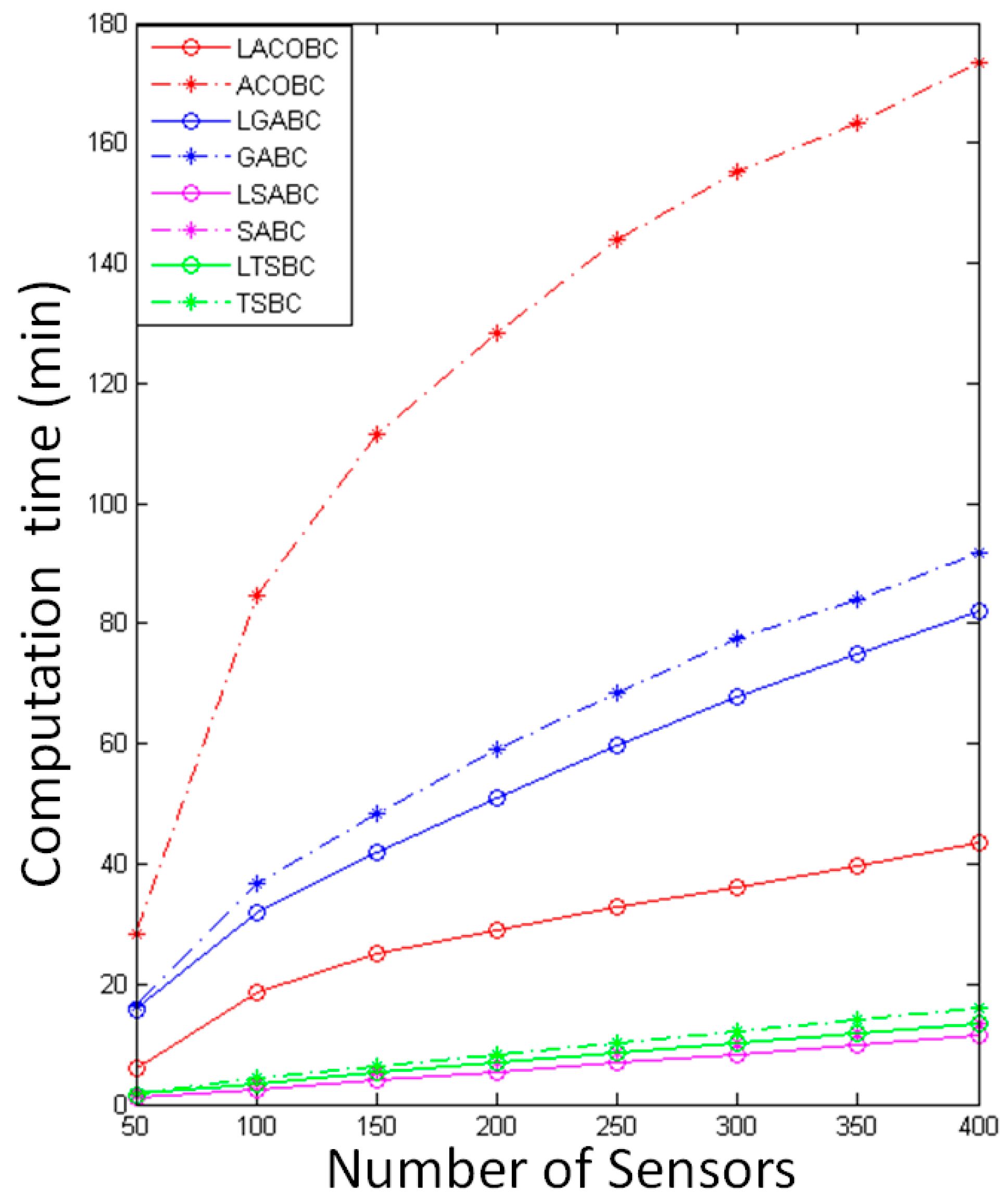
5.4. Comparison of Computational Time
In this section, we compare the computational time while the number of sensor nodes increased from 50 to 400. The x-axis represents the number of sensors, and the y-axis represents computational time. To ensure objectivity and accuracy, all of the algorithms performed 1000 iterations.
In Figure 4, the computational time of LSABC is less than that of SABC because the layoff algorithm can remove unnecessary candidate chargers to reduce computational time. Most of the computational time is used for calculating the covered sensor nodes.
The computational time of LTSBC is less than that of TSBC. The reason is the same as for TSABC; the layoff algorithm can remove unnecessary candidate chargers to reduce computational time. In LTSBC and TSBC, most of the computational time is used for calculating covered sensor nodes and checking the tabu list, so it will take more computational time than TSABC.
In LGABC and GABC, the computational time is used for checking which sensor nodes are covered by candidate chargers. The computational time will increase if more candidate chargers are deployed. The layoff algorithm can improve the convergence of LGABC, so the computational time can be reduced at the same time.
The computational time of LACOBC is less than that of ACOBC; thus, LACOBC will record the CCL in the beginning. However, ACOBC will calculate the number of covered sensor nodes when ants arrive at a new node in every iteration, and it will require more computational time. The difference in computational time between LACOBC and ACOBC will be large if the sensor nodes increase. The layoff algorithm uses the CCL table to record the covered sensor nodes and change the method used to find the solution; this application reduces the computational time.
Obviously, LGABC and LACOBC will require more computational time than LTSABC and LSABC because they are complicated methods. In LTSBC or LSABC, there is only one solution in every iteration, whereas LGABC and LACOBC have multiple solutions in every iteration; therefore, they will require more computational time to find the best solution.
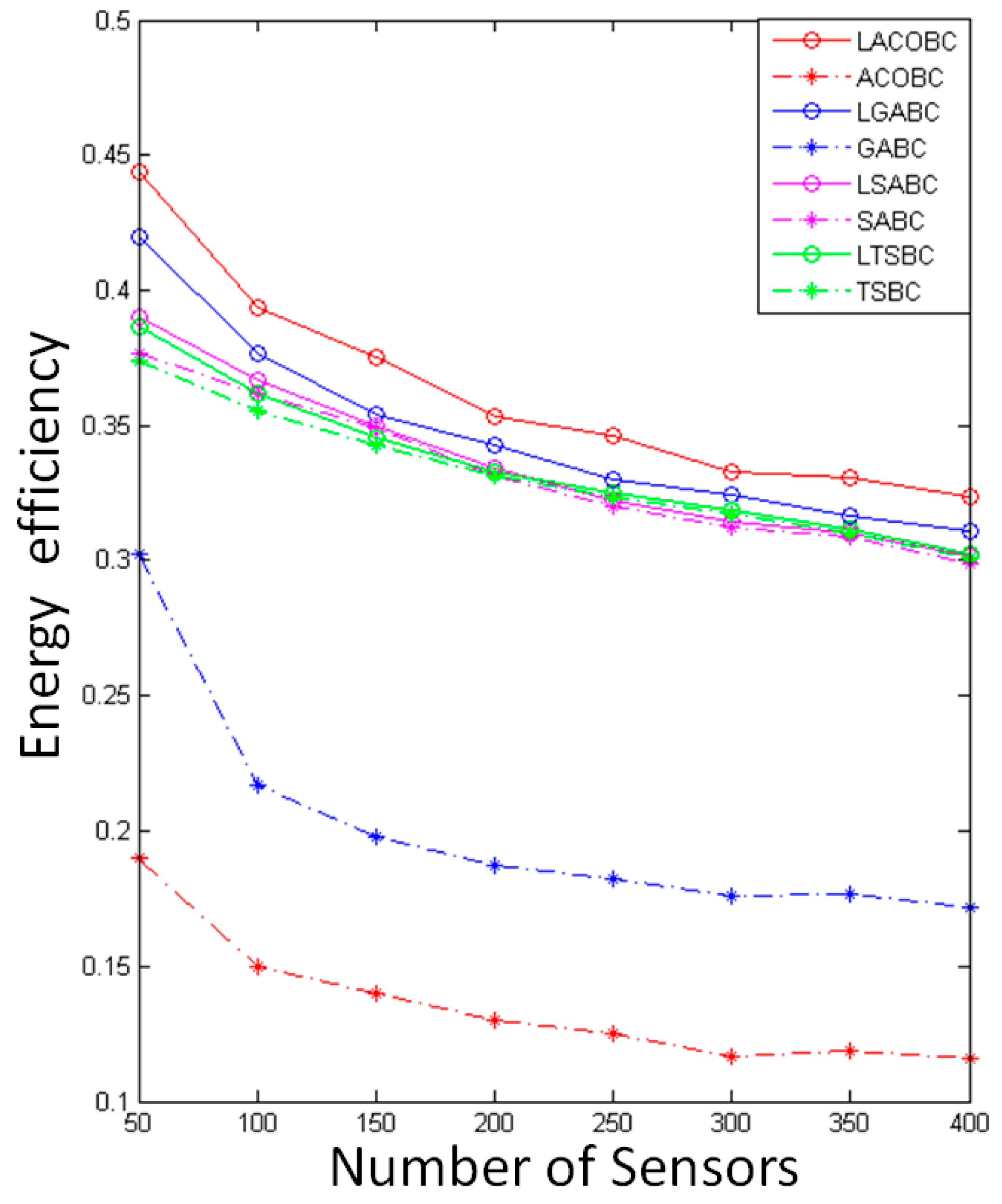
5.5. Comparison of Energy Efficiency
In this section, we compare the energy efficiency while the number of sensor nodes increased from 50 to 400. The x-axis represents the number of sensors, and the y-axis represents computational time. To ensure objectivity and accuracy, all of the algorithms performed 1000 iterations. The energy efficiency was determined by evaluating the power used by the sensor node. It is very wasteful if the sensor node receives too much power; however, it will not run out; conversely, the power will run out completely with insufficient power. This means energy efficiency needs to be good.
Figure 5 shows the comparison of the energy efficiency with original algorithms and layoff versions. The energy efficiency of LSABC is better than that of SABC because LSABC can use fewer chargers to deploy in this environment. In other words, each sensor node can receive enough energy, as there are no useless chargers to add for overlapping areas.
LTSBC uses the layoff algorithm to remove useless chargers and useless sub-solutions at the same time. The simulation showed that LTSBC has better energy efficiency than TSBC because overlapping areas will be decreased through LA.
In the LGABC, the layoff algorithm ensures that all of the sensor nodes will be covered in each iteration, and it will remove useless chargers in the mutation. LGABC can find better solutions through the above-mentioned method. In other words, LGABC can decrease overlapping areas, and the energy efficiency will be increased at the same time.
LACOBC can efficiently decrease the overlapping area. The reason is that LACOBC can check the status of coverage of all the sensors and ensure that LACOBC will not remove the important candidate chargers. For example, there is a sensor node which is only covered by one candidate charger; therefore, we cannot remove this charger because all of sensor nodes should be covered. Obviously, the simulation shows that the LA can enhance ACOBC to find the better solution and decrease overlapping areas.
This simulation showed that the curve of energy efficiency will exhibit negative growth when the number of sensors decreases because the overlapping area will affect the quality of energy efficiency, and overlapping areas increase as the sensor nodes increase in number. The relationship of the number of chargers and energy efficiency is not a positive correlation. If there are many chargers and less overlapping area, it will still have high energy efficiency; this is the reason why energy efficiencies of LSABC and LTSBC will be close to those of SABC and TSBC.
5.6. Comparison of Time Complexity
The time complexity of SABC depends on several factors, such as the amount of input data, the cooling schedule, and the convergence criterion. The main steps of SABC include generating initial solutions, calculating their objective functions’ values, generating neighboring solutions by applying random perturbations and accepting or rejecting them based on a probability determined by the current temperature. The number of iterations required for SABC to converge to a near-optimal solution depends on the cooling schedule and the convergence criterion. The cooling schedule determines the rate at which the temperature is decreased during the search. A slower cooling schedule can result in a longer runtime but can also increase the probability of finding a near-optimal solution. On the other hand, a faster cooling schedule can result in a shorter runtime but can also decrease the probability of finding a near-optimal solution. The convergence criterion determines when the search is terminated. SABC is terminated when the temperature falls below a certain threshold or when a maximum number of iterations is reached. Overall, the time complexity of SABC can be approximated as O(kn), where n is the size of the input dataset and k is the number of iterations required to converge to a near-optimal solution.
The time complexity of TSBC depends on several factors, such as the size of the input dataset, the neighborhood structure and the length of the tabu list. The main steps of TSBC include generating initial solutions, calculating their objective functions’ values, generating neighboring solutions by applying local moves and selecting the best solution based on a tabu search strategy. The time complexity of each iteration of TSBC is O(), where n is size of the input dataset, which corresponds to the time required to evaluate the objective function for the current solution and its neighbors. The neighborhood structure determines the set of moves that can be applied to the current solution to generate neighboring solutions. The time complexity of generating neighboring solutions can vary depending on the complexity of the neighborhood structure. The tabu list is used to avoid revisiting previously visited solutions and to prevent cycling in the search. The length of the tabu list determines the number of solutions that are prohibited from being revisited. The time complexity of maintaining the tabu list can vary depending on the implementation. The number of iterations required for TSBC to converge to a near-optimal solution depends on the convergence criterion and the quality of the initial solution. Overall, the time complexity of TSBC can be approximated as O(), where n is the size of the input data and k is the number of iterations required to converge to a near-optimal solution.
The time complexity of GABC depends on several factors, such as the size of the input dataset, the population size, the crossover and mutation operators and the convergence criterion. The main steps of GABC include generating an initial population, evaluating the fitness of each individual, selecting parents for reproduction, applying crossover and mutation operators to create new offspring and selecting the best individuals for the next generation. The time complexity of each iteration of GABC is O(nm), where n is the size of the input data and m is the time required to evaluate the fitness of an individual. The fitness evaluation involves computing the objective function’s value for each individual in the population. The time complexity of the objective function evaluation can vary depending on the complexity of the problem. The crossover and mutation operators are used to generate new offspring from the selected parents. The time complexity of the crossover and mutation operators can vary depending on the implementation and the complexity of the problem. The number of iterations required for GABC to converge to a near-optimal solution depends on the convergence criterion and the quality of the initial population. The convergence criterion can be based on the number of generations, the fitness improvement or the solution quality. Overall, the time complexity of GABC can be approximated as O(knm), where k is the number of generations required to converge to a near-optimal solution.
The time complexity of ACOBC depends on several factors, such as the size of the input dataset, the number of ants, the pheromone-update rule and the convergence criterion. The main steps of the ACOBC algorithm include generating an initial pheromone matrix, constructing solutions using probabilistic transition rules based on the pheromone matrix, updating the pheromone matrix based on the quality of the constructed solutions and repeating the process until convergence. The time complexity of each iteration of ACOBC is O(), where n is size of the input dataset, m is the number of ants and the exponent 2 is due to the need to calculate the transition probabilities for each ant. The pheromone-update rule is used to update the pheromone matrix based on the quality of the constructed solutions. The time complexity of the pheromone-update rule can vary depending on the implementation and the complexity of the problem. The number of iterations required for ACOBC to converge to a near-optimal solution depends on the convergence criterion and the quality of the initial pheromone matrix. The convergence criterion can be based on the number of iterations, the pheromone level or the solution quality. Overall, the time complexity of ACOBC can be approximated as O(), where k is the number of iterations required to converge to a near-optimal solution.
The layoff algorithm can efficiently remove the solution that cannot lead to an optimal solution. It needs to be used with SABC, TSBC, GABC and ACOBC. The time complexity of layoff algorithm can be approximated as O(k), where k is the number of generations required to converge to a near-optimal solution and n is size of the input data. Compared with the algorithm before adding the layoff approach, time complexities are similar to the original algorithm. However, the layoff approach is more efficient in practice, due to its ability to remove unnecessary solutions.
6. Conclusions
In this paper, we aimed to solve on the indoor charging planning problem of WRSNs. Four metaheuristic algorithms and an optimization method were proposed. In the results, we can see that the proposed metaheuristic algorithms can achieve more efficient fixed charger deployment than the original method can. In addition, in the proposed enhancement method, the layoff algorithm can efficiently reduce the number of deployed chargers, guarantee coverage and get a faster convergence rate. Sometimes, some chargers may serve only a few sensors, so such charger deployment is not cost-effective. In future works, WRSN planning in dynamic environments will be considered.
Author Contributions
Conceptualization, H.-C.C.; methodology, W.-C.C.; software, W.-C.C.; validation, H.-H.C. and F.-H.T.; formal analysis, W.-C.C.; writing—original draft preparation, W.-C.C.; writing—review and editing, H.-H.C.; visualization, H.-C.C. All authors have read and agreed to the published version of the manuscript.
Funding
This research received no external funding.
Institutional Review Board Statement
Not applicable.
Informed Consent Statement
Not applicable.
Data Availability Statement
Not applicable, the study did not report any data.
Acknowledgments
This work was supported by the National Science and Technology Council of Taiwan, R.O.C., under Contracts NSTC-111-2221-E-259-007 and NSTC-111-2221-E-259-008.
Conflicts of Interest
The authors declare no conflict of interest.
References
- Yu, C.M.; Chen, C.Y.; Lu, C.S.; Kuo, S.Y.; Chao, H.C. Acquiring authentic data in unattended wireless sensor networks. Sensors 2010, 10, 2770–2792. [Google Scholar] [CrossRef]
- Han, G.; Jiang, J.; Shu, L.; Niu, J.; Chao, H.C. Management and applications of trust in Wireless Sensor Networks: A survey. J. Comput. Syst. Sci. 2014, 80, 602–617. [Google Scholar] [CrossRef]
- Chen, C.Y.; Chao, H.C. A survey of key distribution in wireless sensor networks. Secur. Commun. Netw. 2014, 7, 2495–2508. [Google Scholar] [CrossRef]
- Nia, A.M.; Mozaffari-Kermani, M.; Sur-Kolay, S.; Raghunathan, A.; Jha, N.K. Energy-efficient long-term continuous personal health monitoring. IEEE Trans. Multi Scale Comput. Syst. 2015, 1, 85–98. [Google Scholar] [CrossRef]
- Habib, C.; Makhoul, A.; Darazi, R.; Salim, C. Self-adaptive data collection and fusion for health monitoring based on body sensor networks. IEEE Trans. Ind. Inform. 2016, 12, 2342–2352. [Google Scholar] [CrossRef]
- Yang, D.; Misra, S.; Fang, X.; Xue, G.; Zhang, J. Two-tiered constrained relay node placement in wireless sensor networks: Computational complexity and efficient approximations. IEEE Trans. Mob. Comput. 2011, 11, 1399–1411. [Google Scholar] [CrossRef]
- Cho, H.H.; Chen, C.Y.; Shih, T.K.; Chao, H.C. Survey on underwater delay/disruption tolerant wireless sensor network routing. IET Wirel. Sens. Syst. 2014, 4, 112–121. [Google Scholar] [CrossRef] [Green Version]
- Khan, H.; Hassan, S.A.; Jung, H. On underwater wireless sensor networks routing protocols: A review. IEEE Sens. J. 2020, 20, 10371–10386. [Google Scholar] [CrossRef]
- Tseng, F.H.; Cho, H.H.; Chou, L.D.; Chao, H.C. Efficient power conservation mechanism in spline function defined WSN terrain. IEEE Sens. J. 2013, 14, 853–864. [Google Scholar] [CrossRef]
- Ouyang, W.; Yu, C.W.; Tien, C.C.; Hao, C.W.; Peng, T.H. Wireless charging scheduling algorithms in wireless sensor networks. J. Internet Technol. 2012, 13, 293–305. [Google Scholar]
- Yen, Y.S.; Hong, S.; Chang, R.S.; Chao, H.C. An energy efficient and coverage guaranteed wireless sensor network. In Proceedings of the 2007 IEEE Wireless Communications and Networking Conference, Hong Kong, China, 11–15 March 2007; IEEE: Piscataway, NJ, USA, 2007; pp. 2923–2928. [Google Scholar]
- Huang, D.C.; Tseng, H.C.; Deng, D.J.; Chao, H.C. A queue-based prolong lifetime methods for wireless sensor node. Comput. Commun. 2012, 35, 1098–1106. [Google Scholar] [CrossRef]
- Ren, J.; Zhang, Y.; Zhang, K.; Liu, A.; Chen, J.; Shen, X.S. Lifetime and energy hole evolution analysis in data-gathering wireless sensor networks. IEEE Trans. Ind. Inform. 2015, 12, 788–800. [Google Scholar] [CrossRef]
- He, S.; Chen, J.; Jiang, F.; Yau, D.K.; Xing, G.; Sun, Y. Energy provisioning in wireless rechargeable sensor networks. IEEE Trans. Mob. Comput. 2012, 12, 1931–1942. [Google Scholar] [CrossRef]
- Zhao, M.; Li, J.; Yang, Y. Joint mobile energy replenishment and data gathering in wireless rechargeable sensor networks. In Proceedings of the 2011 23rd International Teletraffic Congress (ITC), San Francisco, CA, USA, 6–9 September 2011; IEEE: Piscataway, NJ, USA, 2011; pp. 238–245. [Google Scholar]
- Hu, C.; Wang, Y. Minimizing energy consumption of the mobile charger in a wireless rechargeable sensor network. J. Internet Technol. 2015, 16, 1111–1119. [Google Scholar]
- Liao, J.H.; Jiang, J.R. Wireless charger deployment optimization for wireless rechargeable sensor networks. In Proceedings of the 2014 7th International Conference on Ubi-Media Computing and Workshops, Ulaanbaatar, Mongolia, 12–14 July 2014; IEEE: Piscataway, NJ, USA, 2014; pp. 160–164. [Google Scholar]
- Liao, J.H.; Hong, C.M.; Jiang, J.R. An Adaptive Algorithm for Charger Deployment Optimization in Wireless Rechargeable Sensor Networks. In Intelligent Systems and Applications; IOS Press: Jhongli City, Taiwan, 2015; pp. 2080–2089. [Google Scholar]
- Jian, W.J.; Cho, H.H.; Chen, C.Y.; Chao, H.C.; Shih, T.K. Movable-charger-based planning scheme in wireless rechargeable sensor networks. In Proceedings of the 2015 IEEE Conference on Computer Communications Workshops (INFOCOM WKSHPS), Hong Kong, China, 26 April 2015–01 May 2015; IEEE: Piscataway, NJ, USA, 2015; pp. 144–148. [Google Scholar]
- Tsai, C.W.; Huang, W.C.; Chiang, M.H.; Chiang, M.C.; Yang, C.S. A hyper-heuristic scheduling algorithm for cloud. IEEE Trans. Cloud Comput. 2014, 2, 236–250. [Google Scholar] [CrossRef]
- Boussaï, D.I.; Lepagnot, J.; Siarry, P. A survey on optimization metaheuristics. Inf. Sci. 2013, 237, 82–117. [Google Scholar] [CrossRef]
- Stielau, O.H.; Covic, G.A. Design of loosely coupled inductive power transfer systems. In Proceedings of the PowerCon 2000. 2000 International Conference on Power System Technology. Proceedings (Cat. No. 00EX409), Perth, WA, Australia, 4–7 December 2000; IEEE: Piscataway, NJ, USA, 2000; Volume 1, pp. 85–90. [Google Scholar]
- Kiani, M.; Ghovanloo, M. The circuit theory behind coupled-mode magnetic resonance-based wireless power transmission. IEEE Trans. Circuits Syst. I Regul. Pap. 2012, 59, 2065–2074. [Google Scholar] [CrossRef] [PubMed] [Green Version]
- Ching, N.N.; Wong, H.Y.; Li, W.J.; Leong, P.H.; Wen, Z. A laser-micromachined multi-modal resonating power transducer for wireless sensing systems. Sens. Actuators A Phys. 2002, 97, 685–690. [Google Scholar] [CrossRef]
- Shinohara, N. Power without wires. IEEE Microw. Mag. 2011, 12, S64–S73. [Google Scholar] [CrossRef]
- Erol-Kantarci, M.; Mouftah, H.T. Suresense: Sustainable wireless rechargeable sensor networks for the smart grid. IEEE Wirel. Commun. 2012, 19, 30–36. [Google Scholar] [CrossRef]
- Chiu, T.C.; Shih, Y.Y.; Pang, A.C.; Jeng, J.Y.; Hsiu, P.C. Mobility-aware charger deployment for wireless rechargeable sensor networks. In Proceedings of the 2012 14th Asia-Pacific Network Operations and Management Symposium (APNOMS), Seoul, Republic of Korea, 25–27 September 2012; IEEE: Piscataway, NJ, USA; pp. 1–7. [Google Scholar]
- Pang, Y.; Zhang, Y.; Gu, Y.; Pan, M.; Han, Z.; Li, P. Efficient data collection for wireless rechargeable sensor clusters in harsh terrains using UAVs. In Proceedings of the 2014 IEEE Global Communications Conference, Austin, TX, USA, 8–12 December 2014; IEEE: Piscataway, NJ, USA; pp. 234–239. [Google Scholar]
- Tian, Y.; Cheng, P.; He, L.; Gu, Y.; Chen, J. Optimal reader location for collision-free communication in WRSN. In Proceedings of the 2014 IEEE Global Communications Conference, Austin, TX, USA, 8–12 December 2014; IEEE: Piscataway, NJ, USA; pp. 4418–4423. [Google Scholar]
- Rault, T.; Bouabdallah, A.; Challal, Y. Multi-hop wireless charging optimization in low-power networks. In Proceedings of the 2013 IEEE Global Communications Conference (GLOBECOM), Atlanta, GA, USA, 9–13 December 2013; IEEE: Piscataway, NJ, USA; pp. 462–467. [Google Scholar]
- Hu, C.; Wang, Y. Minimizing the number of mobile chargers in a large-scale wireless rechargeable sensor network. In 2015 IEEE Wireless Communications and Networking Conference (WCNC), LA, USA, March 2015; IEEE: Piscataway, NJ, USA, 2015; pp. 1297–1302. [Google Scholar]
- Shu, Y.; Yousefi, H.; Cheng, P.; Chen, J.; Gu, Y.J.; He, T.; Shin, K.G. Near-optimal velocity control for mobile charging in wireless rechargeable sensor networks. IEEE Trans. Mob. Comput. 2015, 15, 1699–1713. [Google Scholar] [CrossRef] [Green Version]
- Chien, W.C.; Chang, Y.C.; Lin, Y.S.; Lai, C.F.; Chao, H.C. Intelligent Power Charging Strategy in Wireless Rechargeable Sensor Network. In Proceedings of the 2019 23rd International Computer Science and Engineering Conference (ICSEC), Phuket, Thailand, 30 October–1 November 2019; IEEE: Piscataway, NJ, USA; pp. 246–250. [Google Scholar]
- Chen, Y.C.; Jiang, J.R. Particle swarm optimization for charger deployment in wireless rechargeable sensor networks. In Proceedings of the 2016 26th International Telecommunication Networks and Applications Conference (ITNAC), Dunedin, New Zealand, 7–9 December 2016; IEEE: Piscataway, NJ, USA; pp. 231–236. [Google Scholar]
- Brooks, S.P.; Morgan, B.J. Optimization using simulated annealing. J. R. Stat. Soc. Ser. D 1995, 44, 241–257. [Google Scholar] [CrossRef]
- Glover, F. Tabu search—Part II. ORSA J. Comput. 1990, 2, 4–32. [Google Scholar] [CrossRef] [Green Version]
- Holland, J.H. Adaptation in Natural and Artificial Systems: An Introductory Analysis with Applications to Biology, Control, and Artificial Intelligence; MIT Press: Cambridge, MA, USA, 1992. [Google Scholar]
- Cheng, S.T.; Hsu, C.L. Genetic optimal deployment in wireless sensor networks. J. Internet Technol. 2005, 6, 9–18. [Google Scholar]
- T’kindt, V.; Monmarché, N.; Tercinet, F.; Laügt, D. An ant colony optimization algorithm to solve a 2-machine bicriteria flowshop scheduling problem. Eur. J. Oper. Res. 2002, 142, 250–257. [Google Scholar] [CrossRef]
Figure 1.
The chargers were deployed on the ceiling.

Figure 2.
Deployment diagram.

Figure 3.
Comparison of the number of chargers.

Figure 4.
Comparison of computational time.

Figure 5.
Comparison of energy efficiency.


Table 1.
Simulation parameters.
| Parameters | Values |
|---|---|
| Size of the venue The number of sensor nodes Effectual charger distance CPU | 30 × 25 × 3 50–400 5 m i5-11400 |
| RAM | 16 G |
| Simulator | Matlab (Version 7.11, R201b) |
Disclaimer/Publisher’s Note: The statements, opinions and data contained in all publications are solely those of the individual author(s) and contributor(s) and not of MDPI and/or the editor(s). MDPI and/or the editor(s) disclaim responsibility for any injury to people or property resulting from any ideas, methods, instructions or products referred to in the content. |
© 2023 by the authors. Licensee MDPI, Basel, Switzerland. This article is an open access article distributed under the terms and conditions of the Creative Commons Attribution (CC BY) license (https://creativecommons.org/licenses/by/4.0/).
Share and Cite
MDPI and ACS Style
Cho, H.-H.; Chien, W.-C.; Tseng, F.-H.; Chao, H.-C. Artificial-Intelligence-Based Charger Deployment in Wireless Rechargeable Sensor Networks. Future Internet 2023, 15, 117. https://doi.org/10.3390/fi15030117
AMA Style
Cho H-H, Chien W-C, Tseng F-H, Chao H-C. Artificial-Intelligence-Based Charger Deployment in Wireless Rechargeable Sensor Networks. Future Internet. 2023; 15(3):117. https://doi.org/10.3390/fi15030117
Chicago/Turabian StyleCho, Hsin-Hung, Wei-Che Chien, Fan-Hsun Tseng, and Han-Chieh Chao. 2023. "Artificial-Intelligence-Based Charger Deployment in Wireless Rechargeable Sensor Networks" Future Internet 15, no. 3: 117. https://doi.org/10.3390/fi15030117
Note that from the first issue of 2016, this journal uses article numbers instead of page numbers. See further details here.