

A Petri Net Model for Cognitive Radio Internet of Things Networks Exploiting GSM Bands †


Department of Engineering, University of Messina, C.da Di Dio (Villaggio S. Agata), 98166 Messina, Italy
*
Author to whom correspondence should be addressed.
†
This paper is an extended version of our paper published in 2019 International Conference on Computing, Networking and Communications, ICNC 2019, “A full secondary user model for cognitive radio in a GSM-900 scenario”.
‡
These authors contributed equally to this work.
Future Internet 2023, 15(3), 115; https://doi.org/10.3390/fi15030115
Submission received: 20 February 2023
/
Revised: 13 March 2023
/
Accepted: 16 March 2023
/
Published: 21 March 2023
(This article belongs to the Special Issue Future Communication Networks for the Internet of Things (IoT))
Abstract
:Quality of service (QoS) is a crucial requirement in distributed applications. Internet of Things architectures have become a widely used approach in many application domains, from Industry 4.0 to smart agriculture; thus, it is crucial to develop appropriate methodologies for managing QoS in such contexts. In an overcrowded spectrum scenario, cognitive radio technology could be an effective methodology for improving QoS requirements. In order to evaluate QoS in the context of a cognitive radio Internet of Things network, we propose a Petri net-based model that evaluates the cognitive radio environment and operates in a 200 kHz GSM/EDGE transponder band. The model is quite flexible as it considers several circuit and packet switching primary user network loads and configurations and several secondary user types of services (that involve semantic transparency or time transparency); furthermore, it is able to take into account mistakes of the spectrum sensing algorithm used by secondary users. Specifically, we derive the distribution of the response time perceived by the secondary users, where it is then possible to obtain an estimation of both the maximum throughput and jitter. The proposed cognitive radio scenario considers a secondary user synchronized access to the channel when using the GSM/EDGE frame structure.
1. Introduction
Internet of Things (IoT) is a system of interconnected digital objects that provide things with the ability to transmit and receive data without human operation. IoT has rapidly evolved; nowadays, it touches most of our daily life. Smart lamps, smart switches, smart thermostats, smart opening drives, smart loudspeakers, smart microphones, and smart cameras are just some of the devices which can be automatically involved in managing specific scenarios of our life. Most IoT devices use a wireless link in order to communicate due to the increased versatility and ease of installation. The rapid growth of such IoT device installations is generating a high crowding of the spectrum due to the huge number of packets produced per unit time. Cognitive radio (CR) technology allows for these problems to be overcome thanks to the possibility of using the spectrum resource in a shared way. Machine learning approaches, usually based on deep reinforcement learning and federated learning, have been extensively investigated as of late for intelligent resource allocation in cognitive radio environments and IoT systems [1,2,3,4]. The integration of IoT and CR technology is termed in the literature as Cognitive Radio Internet of Things (CRIoT) [5].
IoT wireless technologies can be classified in terms of the radio range:
- Long radio range: the device usually leverages a licensed band of cellular networks, and as such, it could be expensive; LoRa (short for long range) and satellite are also used technologies;
- Medium radio range (no greater than 100 m): the most common radio technologies include ZigBee, Wi-Fi, Z-Wave, and thread;
- Short radio range (not exceeding 30 m): the most common radio technologies in use; it includes Bluetooth (or its evolution, Bluetooth LE) and RFID.
The various states regulate wireless networks access for public radio communication by means of theirs governmental agencies. The spectrum is assigned to license holder companies on a long-term basis for large geographical regions. Specific portions of the radio spectrum are maintained as unlicensed all over the world thanks to international agreements, such as the industrial, scientific, and medical (ISM) radio bands.
Except in the case of the long radio range, the use of unlicensed bands is the most typical case for wireless communications in the IoT environment. These unlicensed subbands are suitable for building services, having flexibility and low cost without any restrictions on the wireless coverage and network topology. Accordingly, these bands have often been overcrowded due to several wireless technologies. For instance, the ISM band at GHz is used by many cordless telephones, baby monitors, WPANs (wireless personal area networks such as Bluetooth Low Energy), Bluetooth, ZigBee/IEEE 802.15.4 WSNs (wireless sensor networks), WLANs (wireless local area networks such as IEEE 802.11-based networks), WiMAX (worldwide interoperability for microwave access), and even microwave ovens, which operate by emitting a very high power signal in the same band.
Conversely, as shown by various measurement campaigns conducted by agencies such as the Federal Communications Commission (FCC) in the United States and in the United Kingdom, the assigned frequency bands are not used at all times and in all places by primary users (PUs) [6,7]. For example, as shown by the measurement results reported in [8], the uplink channel (UL) of the 850 MHz GSM band has, on average, a less than duty cycle over a 24 h period measurement time [7].
CR technology can be used with the goal of achieving the dual purpose of both reducing the occupancy of overcrowded unlicensed ISM bands and increasing the utilization of licensed bands without disrupting the primary user [9]. CRs can be used, for instance, to gain more bandwidth for the bandwidth-hungry multimedia applications [10]. Considering the high level of user migration from 2G to 3G/4G and 5G technology, the GSM band shows a lower occupancy level; therefore, it is better suited for a range of CR services [11,12,13].
GSM stands for the Global System for Mobile Communications, and it is the world’s most popular cellular communications system. As shown in Table 1, GSM operates in various bands. At the beginning of 1997, the European Telecommunications Standards Institute (ETSI) introduced the Enhanced Data Rates for the GSM Evolution (EDGE) to evolve GSM toward third-generation capabilities; starting with the General Packet Radio Service (GPRS) and circuit switched data (CSD), the following enhanced versions were proposed: EGPRS and ECSD.
GSM uses a combination of Time-Division and Frequency-Division Multiple Access (TDMA/FDMA). Both the uplink and downlink bands are partitioned in 200 kHz channels. Each channel is divided into eight time slots. Slow frequency hopping can be used to alleviate multipath fading. To reduce interference and battery consumption, GSM devices can make use of power control and discontinuous transmission. Technically, EDGE is primarily a radio interface improvement of GSM/GPRS. The EDGE physical layer parameters appear as almost identical to those of GSM; specifically, the carrier spacing is again 200 kHz, and the TDMA frame structure is unchanged.
Although whole channels may be unused at certain times (e.g., at night), a CR device could potentially use unused time slots due to a low-traffic condition or discontinuous transmission. In this case, the approach used by SUs is called the overlay model in contrast to the underlay model; in the latter, SUs and PUs can coexist and share the same spectrum with each other by employing Code Division Multiple Access (CDMA), which was used starting from 3G technology, as long as the interference caused by the SUs to PUs is less than the predefined system threshold [14].
The locations of the base stations are usually fixed and depend on the chorography and population density of the specific area. Regardless of this fix positioning of the base stations, one should consider that the mobile operator could decide to switch on a base station in a specific location only for the time length of an event where the presence of a high aggregation of people is expected for a limited time (e.g., a sport event or a live concert). However, mobile locations are not known and often move at a high speed, e.g., in trains or cars, making it difficult for CR devices to avoid interfering with PUs [15].
As in any other packet-switched network, the quality of service (QoS) in a CR network will be affected by three main parameters: throughput (the rate of user data output from a channel averaged over a time interval), time delay (the elapsed time between the instant when the packet arrives at the head of the SU transmitting queue until the instant its transmission ends), and jitter (the range of the time delay over the duration of the communication) [16,17,18]. The study of these metrics is particularly important for establishing the QoS in a CRN because they are always affected by the PUs’ level of activity [19]. On the other hand, the system complexity makes it rather difficult to derive performance measures through a well established modeling paradigm. We chose Petri nets (PNs) as a modeling paradigm because it is rather natural and simple to represent both parallelism and synchronization with the networks; at the same time, PNs are able to design complex system models in a very easy way through the use of interacting sub-models. This latter feature becomes very important in the context of packet-based wireless systems like the system analyzed here, especially because we want to study the PU behavior when both circuit switching and data packet switching services are implemented in the same base station. Moreover, the non-Markovian stochastic Petri net (NMSPN) class was used to exploit two of their main features: (1) the ability to correctly represent non-exponentially distributed time events; and (2) the memory policies for modeling suspend/resume behaviors.
In this work, we characterize both the throughput and time delay of a cognitive radio network operating in a GSM channel using an NMSPN model of the traffic that is generated by the PUs. Specifically, in order to reduce interference with PUs, our approach takes into account synchronized SUs, which are able to recognize the GSM time slot boundaries. In order to avoid interference with the PUs, each SU device must listen to the channel at the start of each slot, and it can only begin transmission if it verifies no PU activity. Moreover, the frame length of each SU must not span over the final boundary of the slot; accordingly, several frames will be necessary to transmit a single information unit.
In [20], we already proposed the same approach in order to characterize both the throughput and time delay of a cognitive radio network operating in the channel of a GSM transponder. In this work, we introduced the modeling of the discontinuous transmission to better characterize the behavior of speech phone calls, and we mostly extended the previous model in order to take into account both the circuit switching and packet switching traffic of a GSM/EDGE transponder.
The rest of the paper is organized as follows. In Section 2, we analyze the most relevant works related to this research. In Section 3, we characterize the cognitive environment through the analysis of the primary and secondary users transmission methods. The NMSPN models used to capture the behavior of the cognitive environment and evaluate the QoS are introduced in Section 4. Section 5 describes the results obtained by evaluating the models; finally, Section 6 concludes our work.
2. Related Works
A relatively recent paper [21] studied the service time required to transmit a packet in a cognitive radio scenario in the GSM band. The authors considered an exclusive use of the channel by an SU to transmit its packet without allowing spectrum handoff during the transmission. The authors derived the service time distribution of the SUs, taking into account the PU interruptions. The authors considered a time unit for time accounting purposes; these time units were not synchronized with the time slotting process of the GSM time-division multiplexing. Furthermore, the authors assumed that the spectrum sensing was available in the beginning of each time unit and neglected this sensing duration. Although they assumed that their approach could be applicable for a non-null spectrum sensing duration, in this paper, we argue that a synchronization mechanism between the SU and PU is necessary to avoid or reduce disruptive collision generated by the SUs traffic.
The authors of [22] focused on the continuous sensing technique to guarantee no interference caused by SUs. An SU continuously senses the channel while transmitting or waiting; it starts its transmission immediately when the channel becomes available and stops it as soon as the PU re-occupies the channel. The SU is able to transmit using different modulation schemes, obtaining a different rate according to the channel condition. The authors modeled the PU behavior by means of a two-state Markov chain, where the transmission slot (the continuous period of time during which the channel is available for SU transmission) and the waiting slot (the continuous time period in between the two transmissions) were modeled as exponential random variables. Moreover, they assumed that the transmission rate can only change in different transmission slots (i.e., it remains unchanged in the same slot). It appears evident that this approach does not accurately match the behavior of a GSM PU, which occupies the channel using slotted periodical multiplexing.
In [23,24], the authors modeled the PU behavior by means of a continuous Markov model while the SU continuously monitored PU activity during transmission; when not transmitting, it was able to adopt a continuous or periodic sensing mode. For both continuous sensing and periodic sensing, the authors obtained analytical results for the probability distribution of the extended delivery time while considering an M/G/1 queuing setup at the SU transmitter.
The authors of [25] simultaneously used the TDMA and FDD features of GSM for the first time to enhance the spectrum access performance of CR. They analyzed four different dynamic spectrum access scenarios: (1) when both the PU and BS were outside of the SU transmission range; (2) when only the PU node was located outside of the SU transmission range; (3) when the PU node was within the SU transmission range, while the BS was located outside; and (4) when both the PU and BS were located within the SU transmission range. The authors provided two analytical models when the SUs were near the PU and when the SUs were near the BS to obtain the TDMA channel idleness duration. In the first case, the authors evaluated the available time duration for SU transmission, starting from the probability to have p PUs inside the area covered by the transmission range of am SU. In the second case, they assumed that the PU packet arrivals followed a Poisson distribution and that the PU packet service time followed an exponential distribution. The GSM primary network was modeled by a finite-state Markov chain, which characterized the state with the number of active PUs in the system. However, the proposed model did not seem to catch the behavior of a typical switching circuit service used in GSM technology [26].
The GSM spectrum availability in Aivero, Portugal was analyzed in [27]. In this paper, the authors concluded that the distribution of time periods in GSM900 has an exponential behavior and that the GSM900 spectrum is not usable for opportunistic usages due to the high occupancy; in our opinion, these results must be carefully considered because they were obtained in 2011 when the use of 3G was not heavy yet. The traffic and duty cycle patterns in GSM900 in seven different European locations were also analyzed in [28]. The authors performed synchronized measurements and pointed out that the actual activity patterns can have significant variations. Accordingly, the design of secondary users should avoid a simplified assumption of the traffic patterns. The authors of [29] performed a similar work in India, considering four different scenarios (both outdoor and indoor). Specifically, they measured a spectrum occupancy for a GSM900 no greater than in uplink and between and in downlink.
Ref. [30] is one of the most recent works that addresses the problem of identifying the GSM signal. Using the Kolmogorov–Smirnov test as a decision criteria, the authors performed an identification using the magnitude of the observed signal samples in terms of its cumulative distribution function. They obtained an identification score of approximately with an observation period of 200 μs using both an AWGN channel with an SNR equal to 2 dB and a ITU-T pedestrian A fading channel with an SNR equal to 15 dB. With this fast identification, SUs could be able to use one half of each time slot when PUs are identified as inactive. A demo implementing spectrum sensing and interaction with GSM BSs using SDR devices has been presented in [31]. Moreover, in [19,32], the spectrum sensing was performed using an SDR device; specifically, it was a Universal Software Radio Peripheral (USRP) model B100 device manufactured by Ettus Research. The authors used the spectrum sensing procedure in order to characterize the periods of time when the channel was used by the GSM radio system and to validate their theoretical model for the distribution of SUs packet service delivery time.
Since their introduction in the Carl Adam Petri’s seminal work [33], Petri nets have been widely used for representing a large number of systems in very different fields, such as computer engineering, biology, economy, and telecommunications. Their use in telecommunication systems is quite relevant thanks to their ability to model parallelism and synchronizations together with time delay-characterizing events; thus, they are capable of effectively studying telecommunication infrastructure performances. Many Petri net extensions have been proposed and used over time in order to represent different timings and complex behaviors. Generalized stochastic Petri nets (GSPNs), deterministic and stochastic Petri nets (DSPNs), and fluid stochastic Petri nets (FNSPs) have been exploited in [34] for the study of wireless Internet access systems based on GSM/GPRS technology; the authors’ purpose was to compare the three Petri net approaches to find the most effective one for estimating the performance indices of realistic configurations of GSM/GPRS systems. The evaluated metrics considered in [34] were radio and voice block probabilities and the average number of radio blocks in the base station buffer. The sub-model we propose here is instead designed for evaluating the probability that a slot in the frame is busy because of either a voice call or a data transmission that is in progress because of a PU. As detailed in Section 4.2, these latter probabilities are used in the SU model for deriving SU QoS metrics.
Petri net extensions are also used in [35], where the authors focused on the resiliency of 5G telecommunication networks. Ref. [35] shows how Petri net-based methodologies can be profitably exploited in support of telecommunication network designs despite their complexity. An availability model of 5G networks was proposed, and the system was analyzed at different levels: physical infrastructure, virtual infrastructure, and network services. Conversely, in the approach proposed here, the evaluation is performed by resorting to simulation.
Petri nets have been also extensively used for modeling overall telecommunication networks as well as specific portions of them [36]. Recently, a Petri net extension, generalized nets (GNs), have been used to model part of a more complex telecommunication system [37]. In [37], the authors proposed a GN model based on the classical conceptual model of an overall telecommunication system working both in packet and circuit switching mode and aimed at quality of service estimation. The system was evaluated under stable conditions and focused on the traffic intensity.
In this work, our contribution is related to the use of GSM/EDGE channels by devices acting as SUs in different ways:
- We consider a synchronized access to the channel in order to reduce the probability of collision with PUs;
- We propose a novel model of the GSM/EDGE PU traffic based on a Petri net, which takes into account the transponder load condition (so that it can be tuned in terms of expected load) in terms of the usage of the slotted periodical TDMA by both typical switching circuit and packet switching circuits;
- We also capture specific characteristics of mobile phone calls, such as the discontinuous transmissions obtained in the PU, thanks to the use of a voice activity detector;
- Taking into account a more realistic traffic model, we evaluate the service time and jitter of SUs, and we can validate the results while considering a more accurate distribution of the busy period.
3. Characterization of the Cognitive Environment
In this section, we introduce the telecommunication environment that we assumed as reference in this study; specifically, we describe both the behavior and some technical details of licensed users’ devices, the primary users in Section 3.1. Users’ devices that want to opportunistically access the spectrum, the secondary users, are described in Section 3.2.
3.1. Characterization of the GSM Primary User
GSM is an open, digital cellular technology used for transmitting mobile voice and data services. It uses digital technology and Time-Division Multiple Access (TDMA) transmission methods. A circuit switched system is used for phone calls; it divides each 200 kHz channel into eight 25 kHz time-slots. GSM operates in the 900 MHz and 1.8 GHz bands in Europe and the 1.9 GHz and 850 MHz bands in the US. The 850 MHz band is also used for GSM and 3GSM in Australia, Canada, and many South American countries. To perform frequency reuse and user multiplexing, GSM combines Time-Division and Frequency-Division Multiple Access (TDMA/FDMA). The FDMA part involves the division by frequency of the (maximum) 25 MHz bandwidth into 124 carrier frequencies spaced 200 kHz apart. Depending on the expected load in a specific area, one or more carrier frequencies are assigned to each base station. Each of these carrier frequencies is then divided in time using a TDMA scheme. The fundamental unit of time in this TDMA scheme is called a time slot (or burst period), and it lasts ms ≈ 0.577 ms. Eight burst periods are grouped into a TDMA frame ( ms ≈ 4.615 ms), which forms the basic unit for the definition of the logical channels. One physical channel is one burst period per TDMA frame. Figure 1 shows the frame structure adopted in GSM900. The organization of the frames in multiframe and superframe levels is out of the scope of our work. When operating in downlink, Time Slot 0 (TS0) is always used to transmit the beacon logical channel (base control channel), which is made up of FCCH (frequency correction channel), SCH (synchronization channel), and BCCH (broadcast control channel). When operating in uplink, TS0 is always used to transmit the logical channel RACH (random access channel). The slots from TS1 to TS7 are usually used to transmit the TCHs (transportation channels) in both downlink and uplink modes; a specific cell configuration can be set in such a way that TS1 is used in downlink to accommodate the SDCCH (stand-alone dedicated control channel) and TS8 in frame 12 is used to accommodate the SACCH (slow associated control channel).
Optionally, within an individual cell, TDMA is combined with a slow frequency hopping to address the problems of frequency-selective fading and co-channel interference. In a pre-calculated sequence of different frequencies (algorithm programmed in mobile station), one hop per frame can occur. Our current model of PUs does not take into account frequency hopping.
Moreover, GSM implements discontinuous transmission (DTX) in TCH. When DTX is in operation, the transmitter is switched off if no speech is present; this increases system capacity by reducing the co-channel interference, and it also reduces transmitter power consumption (an important consideration for handheld portables). In a typical conversation, each speaker talks for less than of the time, and it has been estimated that DTX could approximately double the capacity of the radio system [38,39,40]. The DTX mechanism can be implemented thanks to the presence of a voice activity detector (VAD) block, which is able to analyze the activity status of the speaker through the analysis of the speech signal.
The first evolution of the GSM standard provides data services with user bit rates of up to kb/s for circuit switching (CS) data and up to 22.8 kb/s for packet switching data through the General Packet Radio Service (GPRS). Both services are based on the original Gaussian minimum shift keying (GMSK) modulation.
With the introduction of EDGE, two types of transceivers can be used in a cell: standard GSM transceivers and EDGE transceivers. Each time, the slot used for traffic in the cell can be assigned to support one of the possible services:
- GSM;
- CSD;
- GPRS;
- Enhanced CSD (ECSD);
- Enhanced GPRS (EGPRS).
Standard GSM transceivers only support the first three service types, whereas EDGE transceivers support all five. The time slots can be dynamically assigned to each service according to the needs of the cell. Thanks to the introduction of the 8-PSK modulation scheme, EDGE transceivers permit the transmission at a rate of 69.2 kb/s in a single time slot. The time slot format for EDGE (Figure 2) is very similar to that of GSM; specifically, the time length is the same, and it carries 8-PSK symbols instead of GMSK ones. Figure 3 shows some examples of time slots allocation in GSM and EDGE transceivers.
3.2. Characterization of the Secondary User
Our cognitive environment proposal is composed of a CRIoT network with several devices disseminated inside the coverage area of a GSM cell.
Indeed, the use of a heterogeneous wireless sensor network (WSN) that links a wide range of intelligent sensors and actuators has become the cornerstone for IoT-based systems [41]. In the classical application, sensed data and/or human commands are collected and sent to the cloud or to the edge of the network where a dedicated service is running. In this latter scenario, the server usually stores data, somewhat processes it, and sends back some specific commands or sends back data flow to the actuators. Recently, architectural approaches that try to minimize the amount of transferred data in the Cloud–Edge–IoT continuum have been proposed; these approaches also permit the reduction of temporal and throughput requirements [42,43]. During their normal operating, an IoT device uses a radio technology based on an ISM band (WiFi, for example). Due to the presence of others wireless networks in the same area using the same unlicensed band, the band can become overcrowded and, accordingly, a degradation of the quality of experience (QoE) can occur [18,44,45]. Moreover, the WiFi service can be interrupted due to, for example, AP trouble or the Internet connection going down. Once one of these conditions has been detected, the devices of the CRIoT network can decide to use the licensed GSM band as SUs.
One of the possible topologies considers a star or mesh network in which the SU sink node is allocated in the GSM base transceiver station (BTS). Using this kind of topology, the SU sensor nodes can sense environmental variables or acquire human commands and opportunistically transmit them using the GSM band. Likewise, the cloud/edge service can reply with commands or have data flow to the SU actuators using the reverse path.
The GSM operator, allocating the sink node in the BTS, can offer a free or a charge service that does not interfere with the primary GSM service. Privates can exploit this service by installing SU nodes in the cell coverage area, which operate according to the cognitive access rules.
In our approach, each SU must be able to synchronize itself with the GSM frame structure. Thanks to this synchronization, it is possible to detect the boundaries of each single time slot. Once the SU is synchronized, it can run a spectrum sensing algorithm [19,46,47,48] when a new slot starts. Accordingly, it is possible to detect if the channel will be busy in the current time slot due to the transmission of a PU. If the channel is detected to be vacant and the SU has something to be transmitted, it can access the channel and perform the transmission until the end of the current time slot; otherwise, it needs to wait until the beginning of the subsequent time slot.
The SU sensing algorithm can slip into two different kinds of errors: (1) the channel is detected as free, but a PU is actually using it; (2) the channel is detected as busy, but nobody is using it. The first error is the worst because SUs can destroy PUs’ information. Therefore, it is important to reduce this error to the minimum. However, when this kind of error occurs, the SU’s IU will be destroyed as well. Here, we assume that the SU application protocol is able to detect such a situation and retransmits the collided IUs. The second error implies a non-efficient use by the SUs with respect to the band left free by the PUs. When more than one SU in the same coverage area detects the channel that is free in the same time slot, they will access the channel at the same time, and the transmissions will be destroyed due to collision. This latter condition could be mitigated by means of an SU protocol that is able to resolve or prevent collisions (for example, using an ALOHA approach, a CSMA (1-non-p-o)-persistent approach, or a time-division synchronized access).
In order to obtain a good prediction of SUs QoS metrics and, accordingly, the QoE offered by the CRIoT, it is necessary to consider at least the first two errors in the model (the last one is specific of SUs network, and for comparison purposes, it can be considered null). In this context, one of the most important metrics to evaluate is the response time. This is defined as the time elapsing from the moment the client initiates the request until the moment the client receives the response with the payload. From the knowledge of the distribution of the response time, it is possible to evaluate two important QoS parameters: the expected maximum throughput the SU may achieve and the expected maximum jitter. Accordingly, important information related to the use of the CRIoT to support real time services can be derived. Thus, the response time provides relevant information for evaluating the QoE of the CRIoT networks when the SUs transmit over a typical GSM cellular channel.
4. QoS Evaluation of Secondary User Based on NMSPNs
The interactions between the PUs and SUs in the GSM-based cognitive environment will be modeled by a class of stochastic PN model [49]. We chose PNs as the modeling tool because of their ease in representing synchronizations and parallelism, even in complex systems. In order to improve model expressiveness, several extensions have been introduced to stochastic PNs over time. Specifically, we used non-Markovian SPN (NMSPNs) [50] with enabling functions, deterministic events, and memory policies [51] to appropriately model the effects of preemption during data transmissions.
An NMSPN is an SPN in which the time evolution of the marking process can be more general than a continuous-time Markov chain (CTMC) [52]. It can be defined as a tuple
where
- is the set of places;
- is the set of transitions;
- are, respectively, the input, output, and inhibitor arcs’ functions; they map the transitions to bags of places (a bag is a set in which the replication of elements is allowed, and it keeps track of the “multiplicity” of each element);
- is a function that maps each immediate transition into a constant weight ;
- is a function that maps each timed transition into a cumulative distribution function (CDF) ;
- is a function that maps each timed transition into a preemption memory policy
- is a function that associates a priority to each transition ;
- is the initial marking, i.e., the initial distribution of tokens among the places in , which represents the initial state of the model.
The firing of a transition will occur according to the atomic firing semantics [53]; as soon as a transition is enabled, the future elapsing time occurring until the transition will fire is sampled from the related CDF; the transition will only fire after that time if it will still be enabled. Accordingly, it is possible to have more than one transition enabled at a specific time; the next one to fire will be that with the coming sampled time. After a transition fires, it will be sampled the firing times of the newly enabled transitions, and they will contribute with the previous ones to determine the next transition event (race execution policy [51]). When an enabled transition is preempted without firing, the memory policy determines how the remaining firing time is managed. Due to the memoryless property of the exponentially distributed firing time transitions, memory policies have an effect on the non-exponentially distributed firing time transition (for a more detailed discussion on preemption policies, see [51,52,54]. In our model, we make use of the deterministic transitions and preemption policy, which is able to save the remaining firing time of the deterministic transitions, resuming them when re-enabled.
Our overall model is organized into two interacting NMSPNs as depicted in Figure 4 and Figure 5. Respectively, they represent an EDGE transceiver of a GSM base station used by PUs (which permits both speech phone calls using performing circuit switching access and data transmission using packet switching access) and SUs trying to opportunistically access the same band assigned to the transceiver. We exploited the independence of PUs with respect to the SU in the development of the two models; in fact, when a PU wants to make a call or transmit data, the resources in the base station are reserved for establishing a connection if any slot is free, irrespective of the SUs will. At the opposite end, an SU can only use a time slot if no PU is already using it, making it dependent on the PU’s behavior; this kind of dependency is modeled by exploiting the probability values computed by solving the primary user model into the secondary user model (as explained later).
4.1. The Primary User Model
The model in Figure 4 is used to derive the probabilities at a steady state to find a free slot in a transceiver assuming a given traffic load generated by the GSM users. These probabilities are then used in the NMSPN of Figure 5 to model the PU’s active connections in the system. In this way, we implement the dependency of SUs with respect to PUs. Our transceiver model assumes that the first time slot (TS0) is reserved for signaling, a specific amount of time slots (from TS1 to TS3) are reserved for circuit switching phone calls, and the remaining ones (from TS4 to TS7) can be used for both circuit switching phone calls and data transmission in the packet switching mode. A single GSM/EDGE transceiver model is characterized by five blocks: a block to model the generation of PU phone calls, a block to model the data packet arrival, a block to model the time slots that are only used in the circuit switching mode, a block to model the slots used in both the circuit switching and packet switching modes, and a block to represent the activation of slots in slotted periodical time-division multiplexing (TDM).
The SPEECH WORKLOAD block the models generation of PU phone calls; it is made by the places CS_load and CS_choice and the transitions CS_arrival and CS_reject. Tokens in place CS_load enable the timed transition CS_arrival to fire. In this work, we assume that the PU phone calls arrive according to a Poisson process; thus, the timed transition CS_arrival is an exponential transition with parameter , with being the parameter of the arrival process. The number of tokens N in place CS_load represents the available free slots; thus, when the place is empty, the system is full of calls, and no new call can start. Because we are considering a transceiver that uses TS0 for signaling, only seven calls can be simultaneously managed by a station; thus, we set . When a new call request arrives (firing of CS_arrival), a token is put in place CS_choice and all of the enabled immediate transitions CS_sloti, with corresponding to free slots, are triggered. One of the triggered transitions CS_sloti is randomly selected to fire; we set all their weights to in such a way that the random selection follows a uniform distribution. The transition CS_reject has lower priority than CS_sloti; it only fires when a call arrives (we have a token in place CS_choice) and all of the time slots are busy (we have no transition CS_sloti enabled) emulating the call reject due to system congestion.
The circuit switching speech service is modeled through places CS_busyi, Vi, and Si in order to take into account DTX. A token in place CS_busyi means that the slot i is currently used by a phone call; thus, an inhibitor arc to the transition CS_sloti (and also to PS_sloti in CS+PS slot blocks) ensures that it is disabled the immediate transition for selecting the slot when it is busy. The DTX mechanism is modeled through timed transitions Vi2Si and Si2Vi. One token in place Vi means that the output of the VAD is true (Voice detected) and, accordingly, the time slot is actually used; meanwhile, a token in place Si means that the output of the VAD is false (Silence detected) and, accordingly, no transmission occur in the time slot. According to [40], the duration of the on (talk spurt) and off (silent gap) periods follow exponential distributions with mean and , respectively. We used the timed transition CSi to model the call duration with a mean time equal to . The firing of CSi, which means that the call is over, consumes the token from its input place (CS_busyi and puts a new token in the place CS_endi. Suddenly, the token from one of the two places (Vi or Si) will be removed thanks to the immediate transitions CS_freeVi or CS_freeSi. It is worth noting that only one of the two transitions CS_freeVi and CS_freeSi can be enabled depending on the state of the VAD; their firing puts one token in place CS_load, representing the system state where the slot becomes free.
The data workload block models the data packet arrival for the data packet switching service; it is created by the places PS_load and PS_choice and the transition PS_arrival; tokens in place PS_load enable the timed transition PS_arrival to fire. We assume the packet arrival process to be a Poisson process; thus, the interarrival time is modeled by using an exponential transition with parameter , with being the parameter of the arrival process. The number of tokens M in place PS_load represents the size of the queue buffer in terms of packets; thus, when the place is empty, the queue is full and packets will be discarded. When a new packet arrives (when PS_arrival fires), a token is put in place PS_choice and all the immediate enabled transitions PS_sloti, with corresponding to free CS+PS slots, are triggered. One of the triggered transitions PS_sloti is randomly selected to fire; we set all their weights to in such a way that the random selection follows a uniform distribution. If we have no PS_sloti-enabled transition, the token simply accumulates in place PS_choice, emulating the buffering of the corresponding packet in the queue. As soon as a PS_sloti transition becomes enabled, the corresponding packet transmission starts moving the token to the corresponding place PS_busyi. Indeed, the packet switching service is modeled through place PS_busyi and timed transition PSi. A token in place PS_busyi means that the slot i is currently being used by a packet transmission; thus, an inhibitor arc from this place to the transitions PS_sloti and CS_sloti ensures that the slot cannot be selected for neither a new incoming call nor other data packet transmission. We model the transmission time with an exponential distribution as we consider the message length to be exponentially distributed [55] with mean bit and with the transmission rate constant being equal to bps. We have settled this last value while assuming the average radio interface rate per time slot over all possible channel coding schemes for the EDGE packet switching transmission (CS-1/4, PCS-1/6). Accordingly, we set the expected firing time of the timed transitions PSi to be equal to .
The last block of the model, slot selection, is used to represent the activation of slots; the number of tokens in place enabled_slot models the slots that are actually active, i.e., i tokens in the place means that slot i is the active slot. Instead, place turn is used to count the turns inside a round of N slot activation. The mechanism is implemented as follows. When the round starts, there are zero and eight tokens in places turn and enabled_slot, respectively; the transition nextSlot is enabled until the tokens are in their input place turn. Transition nextSlot is a timed deterministic transition whose firing time is set to the slot length ; because turn is its only input place, it will fire eight times at regular intervals, moving a token from turn to enabled_slot. When all eight slots are moved, the immediate transition reset becomes enabled thanks to its input arc, whose multiplicity is set to eight, and all the tokens are immediately moved into turn, resetting the round. We used the slot selection sub-model to enable the activities in the slots at the correct time period. In fact, the transitions CSi, Vi2Si, Si2Vi, and PSi can only fire when slot i is active; thus, in order to be correctly enabled, we added an enabling function to each of them, as reported in Table 2, where we used the usual notation to denote the number of tokens in place P (An enabling function is a logical condition on a transition that must be true for the transition to be enabled together with the enabling conditions due to its input places).
We used the model in Figure 4 to evaluate the probability that each single slot is free at a stable state. Let with be the probability that the i-th circuit switching dedicated slot is free; it could be evaluated from the model as
For slots exploiting both circuit and packet switching (with ), the probability can be instead evaluated as
Due to the symmetries and the uniform random choice, the probabilities into each category of slots are all equal; thus, it is enough to evaluate only one of them. We denote their values as and , respectively, e.g., we set and .
It is noteworthy that it is possible to simply extend the model to sectors using more than one transponder and to take into account a different number of slots dedicated to the circuit switching service as well.
4.2. The Secondary User Model
The model in Figure 5 has been designed with the aim of evaluating the performance of a secondary user that tries to access a GSM/EDGE transponder band as described in Section 3. It is constituted by two main blocks, which represent the workload generated by the SU (SU workload) and the SU data transmission when a GSM slot is found to be free (SU transmission), respectively. The SU workload block is characterized by two places: population and sending. The former is used to represent the maximum number of IUs managed by the system, and the latter takes into account the number of IUs produced by the SU and waiting to be transmitted. To this aim, until the tokens are in place population, a new IU could be generated and accepted by the system; we limited the number of requests to the buffer size , even if the application would need to send data; if this is the case, the request is lost. It is worth noting that a specific workload profile is modeled by appropriately setting the SU Workload block; it is enough to design a block (it can be arbitrary complex) where the place sending stores tokens representing IUs to send.
In this work, we considered an SU workload (Figure 5) characterized by a Poisson arrival process and consistently sized IUs. This choice has been made to capture the behavior of a typical IoT source, and it was only adopted as an example as also reported in other studies. Specifically, it can also model other specific sources, such as Voice over IP [56,57], flows obtained by frame aggregation techniques, and optimal frame size adaptation [58] for IEEE 802.11x WLANs [59,60]. It is important to highlight that the SU traffic model is arbitrary for the proposed approach; the user can change it to their liking, setting the distributions of both the arrivals and the IUs size according to the specific behavior of the SUs that need to be modeled. According to our choice of SU workload, we set the firing time of transition IUgen to an exponentially distributed random variable (r.v.) with parameter and we set the firing time of the deterministic transition End to a constant value , which expires based on the channel availability, as will be subsequently described.
Until there is space to store new frames, place population is not empty, the transition IUgen is enabled, and it will fire, adding a new token in place sending. In our approach, the model could be extended to represent other workload profiles. In principle, any SU workload block can be used with the only requirements being to have the places population and sending (with the meaning introduced above), which are connected to the SU transmission block as in Figure 5.
The SU transmission block is designed to model the transmission of IUs. Our idea is based on the transition End; it is a deterministic transition whose delay is computed while considering the size of an IU and the SU transmission bit rate . If all of the transponder slots were available, the delay that needed to sent an IU will be ; however, in the cognitive environment, some slots are useless because they are used by PUs, and free slots are partially used by the SU to run the detection algorithm for checking the slot status, as described in Section 3. When place sending has tokens, transition End is enabled; during the enabling period, the time advances, and the transition will fire after time instants. Sometimes, the transition is disabled because either the checking algorithm found the slot busy (token in place wait), or it found the slot erroneously free and the SU transmission collided with the PU transmission (token in place btransm; we assumed that the SU application is able to detect collisions). During the disabling time intervals, the passed amount of time has to be remembered, and the time progress has to start from this latter value. To this aim, we set the preemptive resume memory policy (prs) of the NMSPNs [52] to the transition End that is coherent with the SU behavior, otherwise the firing delay would not reflect the real SU activity. Furthermore, we used three inhibitor arcs to suspend the enabling of End in the relevant states mentioned above.
The remaining part of the NMSPN selects the state of the current slot. When the system starts, seven tokens are in place starting, and one of the two transitions primary and secondary will be enabled according to the values of their associated enabling functions (Table 2). If place sending is empty, primary will fire, moving one token to the place busy. This enables the timed transition Tslot, a deterministic transition whose delay is equal to the slot time (). During this time interval, both the transitions primary and secondary are disabled. When the time slot expires, Tslot fires and the token moves to the place last. Conversely (if place sending is not empty), when the transition secondary fires, one token is placed into the place attempt and another into the place activity. The latter is used to inhibit the firing of transitions primary and secondary until the current time slot expires. A token in attempt means that the slot status checking algorithm has started (the transition test is enabled). The detection algorithm will use a fraction with of the time slot to run; thus, we set test as a deterministic transition with parameter . The firing of test moves the token to place chk, enabling one of the two pairs of immediate transitions chkTCS and chkFCS (the green couple in Figure 5) and chkTCS+PS and chkFCS+PS (the light blue couple in Figure 5) according to the values of their associated enabling functions (Table 2), i.e., according to the current category of i-th time slot. Transitions chkTCS and chkFCS fire with probability and , respectively. Similarly, if we are managing a circuit and packet switching time slot, the transitions chkTCS+PS and chkFCS+PS are enabled; the transition chkTCS+PS will fire with probability , whereas chkFCS+PS with probability . The firing of one of the two transitions chkFCS or chkFCS+PS means that the slot is busy with the PU; the token will be moved to the place wait, and the timed transition delay will be enabled. We set delay as a deterministic transition with parameter . That is the remaining duration of the time slot. As soon as delay fires, a token will be placed in last and the tokens from activity and wait will be removed. This means that the current time-slot is expired and a new one can start. At the opposite, when one of the two transitions chkTCS and chkTCS+PS fire, it means that the time slot is not busy with a PU, and the token moves to the place free, meaning the SU transmission can start. A token in free enables both the immediate transitions TP and FP; they will fire with probabilities of and , respectively. () is the probability that the checking algorithm evaluates to a true positive (false positive) result. When TP fires, the token is put in the place transm, i.e., the state where the SU correctly detected a free slot; otherwise, it will be put in btransm, i.e., an error state, because it has been detected as a free slot when busy. The NMSPN will remain in the arrived state until the corresponding enabled transition does not fire; both sent and collision are deterministic transitions whose firing time is set to the remaining slot time, i.e., . When sent or collision fires, a token will be placed in last and the tokens from transm/btransm and activity will be removed. This means that the current time slot is expired and a new one can start. When seven tokens are collected in the place last (i.e., all of the seven available traffic time slots in a frame have been managed), the place signaling is enabled. This is a deterministic transition whose firing time is set to the slot time duration . It was only inserted in order to take into account the one time slot inside the frame used for signaling. As soon as signalling fires, the seven tokens will be moved to the place starting and the managing of a new frame starts.
SU Performance Measures
Despite the fact that more measures could be derived from the proposed SU model, we focus on two of them in this work: queue length distribution (and loss probability) and response time distribution. Because the number of the IU stored in the buffer (also considering the IU under transmission) is given by the number of tokens in the place , the system queue distribution length is computed by evaluating
at a stable state. Loss probability is equivalent to the probability that the system cannot accept any new incoming IU because its buffer is full; thus, it is given by .
Let us consider the time from the arrival of an IU into the system to the instant that it is completely delivered, denoting it as . Of course, is a r.v., and its cumulative distribution function is defined as . Computation of requires some modification of the model in order to implement the so-called tagged customer method [61], where a tagged IU is chosen and it is observed from its arrival to its delivery. Figure 6 shows the NMSPN used to accomplish this purpose. The performance model is modified by splitting the place sending into two places so as to allow us to distinguish between the tokens already present in the queue (b_sending) and those that arrived after the insertion of the tagged IU (a_sending). The tagged IU is modeled by the place tc_sending; one token in the place means that the tagged IU is waiting to be delivered. During the time it is waiting, new arrived IUs (tokens in a_sending) will not be served thanks to the inhibitor arc from tc_sending to tc_comp; this will only be able to fire when the tagged IU leaves the system. Transition tc_end is identically set to the transition End, modeling the delay of transmitting the tagged IU and also considering the available portion of slots.
This model describes the view of the tagged IU at its arrival in the system. The remaining tokens, i.e., the remaining possible IUs in the system, will be distributed between the places population and b_sending, which are constrained by . All of these states, with the associate probabilities, are departure states for the tagged customer model. The tagged customer model is solved in transient for each of the possible initial markings to compute the response time distribution as conditioned in the different configurations by evaluating
where with is the state where . The overall distribution will be
5. Numerical Results
In order to evaluate the proposed model, we firstly had to characterize the GSM/EDGE PUs’ phone and data traffic. As specified in Section 4.1, according to [55], we set an exponential distribution of phone call length and packet data size. In order to consider different PU phone traffic loads, we set the average call holding time to 180 s in our experiments ( = 5.5556 × 10⁻³ s−1) and varied the mean rate of the Poisson process modeling call arrivals involving the specific transponder from 6 to 60 calls per hour (6, 20, and 60). Accordingly, we loaded each TCH with 0.043, 0.143, and 0.419 Erlang; as a consequence, the considered system workload was set to 0.3, 1.0, and 3.0 Erlang. The mean duration of the on (talk spurt) period was set to be equal to 1 s, and the mean duration of the off (silent gap) period was set to be equal to 1.35 s, which was the procedure for both in [55].
Regarding the packet switching data traffic, we considered the message length as exponentially distributed with an average length of 1.6 kB ([55]) and an average transmission rate equal to 34.2 kb/s. Accordingly, we set the expected rate of the packet switching data service as = 2.61 s−1. In order to consider different PU data traffic loads, we varied the mean rate of the Poisson process modeling packet arrivals involving the specific transponder in our experiments. Specifically, while taking into account that a single user usually generates an average of 0.(30) packets/s ([55]), we varied the packet switching traffic workload considering , and 4 users ( = 0.(30), 0.(60), 0.(90), and 1.(21) s−1). We solved the PU model, deriving the probabilities and finding a slot free for each time the SU wanted to use it at these different phone and data load conditions. The results are summarized in Table 3 and Table 4.
We used the WebSPN software tool [62] to numerically solve the NMSPN models. WebSPN also provides an analytical solution engine for models with many non-exponentially distributed transitions; thus, we did not need to resort to simulation for deriving the numerical results from the NMSPN models.
The modeled SU node produces an = 8 kbit IU with a mean rate of = 16.64 s−1. We assumed a transmission rate of = 271 kb/s and, accordingly, the deterministic firing time of place End will be = 0.03023 s. Moreover, we assumed that the spectrum sensing algorithm needs 25% of a slot time to run, so we set in the SU model and an accuracy such that .
Figure 7 and Figure 8 show the results obtained in terms of the probability distribution of n IUs in the queue. Specifically, we evaluated the probabilities changing the queue size in the set of values . Each subfigure shows the results for a specific primary circuit switching load and a specific queue size . The primary packet switching load () is depicted by the respective curves in each subfigure, as indicated in the legends. As expected, the distributions are affected by the primary loads for both circuit switching and packet switching. For the lighter packet switching and circuit switching loads (Figure 7a,b and Figure 8a,b, ), the distributions appears to be almost uniform, regardless of the queue size. When setting the primary packet switching load to , the distribution of the enqueued IUs in the secondary user appears to be almost linearly increasing for (Figure 7c,e, ), while it appears to be almost exponentially increasing for the others in terms of the considered queue sizes (Figure 7d,f and Figure 8c–f, ). For higher values of the primary packet switching load (), all of the distributions appear to be exponentially increasing. These conditions means an overload of the SU buffer with a high loss probability as the outcome.
Figure 9 and Figure 10 show the results in terms of the cumulative distribution function (CDF) of the response time. The end of the knee in these curves corresponds to the maximum response time. As in the previous figures, each subfigure shows the results for a specific primary circuit switching load and specific queue size . The primary packet switching load () is depicted by the respective curves in each subfigure, as indicated in the legends. As expected, the knees of the curves move to the right as the queue size increases. Taking into account a primary packet switching load with , it occurs at approximately 0.5 s for (Figure 9a,c,e, ), at 1.0 s for (Figure 9b,d,f, ), at 1.4 s for (Figure 10a,c,e, ), and at 1.8 s for (Figure 10b,d,f, ), regardless of the primary switching circuit load . For the lighter primary packet switching load (), the knee of the curves moves slightly to the left; the moving appears to be higher for higher queue sizes.
We point out that the obtained CDFs are defective because the size of the queue is finite and a loss is experienced in almost all cases. The loss probability is computed by taking into account the probability of having a full queue (i.e., , of Figure 9 and , of Figure 10); we can note that the loss probability corresponds to the value of the complement to 1 of each CDF at infinity (i.e., ). Table 5 summarizes the value of loss probabilities in the different workload conditions that we analyzed when the SU application uses different buffer sizes, as modeled by resorting to different queue sizes . Because the CDFs provide a complete characterization of the response time, it is easy to obtain other information about the SU behavior, such as the mean and variance of the delay to deliver IUs. With this detailed characterization of the response time, it is also possible to evaluate the “average throughput” (as the inverse of the mean value of the response time by the IU size), mean delay (the mean value of the response time), and jitter (as the variance of the response time) of the SU traffic and to characterize the system’s QoS accordingly. All of these values are reported in Table 6, Table 7 and Table 8, respectively.
We derived the results above, which are described only considering one specific set of parameters in terms of PU workload for both the circuit switching and packet switching and the transponder configuration; however, the model is very flexible, and its described analysis can be performed when assuming other working conditions. For these reasons, we think that the proposed model can be considered as a good candidate for tuning SU network parameters in specific GSM/EDGE cognitive radio environments in order to obtain desired QoS levels.
6. Conclusions
In this paper, we proposed a new model based on non-Markovian stochastic Petri nets to evaluate QoS performance metrics in a cognitive radio environment operating in the band of a GSM/EDGE transponder. The proposed model is able to manage different load conditions of the licensed band. Specifically, the PU model is flexible because it can capture the behavior of both the circuit switching and packet switching of the mobile devices operating inside the cell; the number of transport channels operating in the switching circuit mode and in the packet switching mode inside the transponder can also be changed as needed. The workload of each type of source can be varied according to the operating condition of the modeled cell; the average number of arriving phone calls and its average time duration can be increased or decreased, as well as the distributions of packet arrivals and distributions of packet sizes for the packet switching traffic. The conceived cognitive radio scenario assumes a synchronized spectrum sensing with the frame structure of a GSM/EDGE transponder. The SU device is able to detect the activity status of PUs in the early portion of a single time slot and opportunistically use the spectrum in the remaining portion. The SU model is flexible as well, both in terms of the distribution of packet arrivals and the distribution of packet size of the generated workload. Moreover, it is able to capture the interactions with PUs, and it is able to take into account possible spectrum sensing mistakes. Numerical results were obtained by modeling the specific scenario of a transponder with three transport channels operating in the switching circuit mode only (to serve phone call traffic implementing discontinuous transmission) and with four transport channels operating in both the packet switching and circuit switching modes. The SU workload follows a typical profile of an IoT device characterized by a Poisson arrival process of consistently sized IUs. The results, which were obtained by varying both the circuit switching and packet switching load of the PU, show that the proposed model is able to capture most of the operating characteristics of an SU by opportunistically accessing the licensed GSM/EDGE band. Specifically, we show how the throughput is affected by the traffic condition of PUs for several sizes of the SU queue. Moreover, the proposed model allows for the capturing of the service time distribution of IUs, as well; important information related to the delay and jitter of the IUs transmitted by the SUs can be derived by this distribution.
As a future work, we plan to extend the numerical analysis for different workload scenarios and to adapt the model for other PUs in a time-slotted context that is different from GSM/EDGE. We will try to build a model capable of capturing the dynamics of a transponder where the number of channels operating in the switching circuit mode can change over time; that is the current limitation of our proposed model. Comparisons of the proposed Petri net models versus other machine learning-based models and generalized networks will be analyzed.
Author Contributions
Conceptualization, S.S. and M.S.; Software, M.S.; Formal analysis, S.S. and M.S.; Writing—original draft, S.S. and M.S. All authors contributed equally to this work. All authors have read and agreed to the published version of the manuscript.
Funding
This research received no external funding.
Data Availability Statement
Data sharing not applicable.
Conflicts of Interest
The authors declare no conflict of interest.
References
- Grasso, C.; Raftopoulos, R.; Schembra, G.; Serrano, S. H-HOME: A learning framework of federated FANETs to provide edge computing to future delay-constrained IoT systems. Comput. Netw. 2022, 219, 109449. [Google Scholar] [CrossRef]
- Grasso, C.; Raftopoulos, R.; Schembra, G. Smart Zero-Touch Management of UAV-based Edge Network. IEEE Trans. Netw. Serv. Manag. 2022, 19, 4350–4368. [Google Scholar] [CrossRef]
- Li, X.; Fang, J.; Cheng, W.; Duan, H.; Chen, Z.; Li, H. Intelligent power control for spectrum sharing in cognitive radios: A deep reinforcement learning approach. IEEE Access 2018, 6, 25463–25473. [Google Scholar] [CrossRef]
- Giannopoulos, A.; Spantideas, S.; Kapsalis, N.; Karkazis, P.; Trakadas, P. Deep reinforcement learning for energy-efficient multi-channel transmissions in 5G cognitive hetnets: Centralized, decentralized and transfer learning based solutions. IEEE Access 2021, 9, 129358–129374. [Google Scholar] [CrossRef]
- Tarek, D.; Benslimane, A.; Darwish, M.; Kotb, A.M. Survey on spectrum sharing/allocation for cognitive radio networks Internet of Things. Egypt. Inform. J. 2020, 21, 231–239. [Google Scholar] [CrossRef]
- Akyildiz, I.F.; Lee, W.Y.; Vuran, M.C.; Mohanty, S. NeXt generation/dynamic spectrum access/cognitive radio wireless networks: A survey. Comput. Netw. 2006, 50, 2127–2159. [Google Scholar] [CrossRef]
- Gao, J.; Suraweera, H.A.; Shafi, M.; Faulkner, M. Channel capacity of a cognitive radio network in GSM uplink band. In Proceedings of the IEEE International Symposium on Communications and Information Technologies, ISCIT’07, Sydney, Australia, 17–19 October 2007; pp. 1511–1515. [Google Scholar]
- McHenry, M.; McCloskey, D.; Lane-Roberts, G. Spectrum Occupancy Measurements Location 4 of 6: Republican National Convention, New York City, New York; Technical Report; Shared Spectrum Company: Vienna, VA, USA, 2005. [Google Scholar]
- Haykin, S. Cognitive radio: Brain-empowered wireless communications. IEEE J. Sel. Areas Commun. 2005, 23, 201–220. [Google Scholar] [CrossRef]
- Amjad, M.; Rehmani, M.H.; Mao, S. Wireless Multimedia Cognitive Radio Networks: A Comprehensive Survey. IEEE Commun. Surv. Tutor. 2018, 20, 1056–1103. [Google Scholar] [CrossRef]
- Shukla, A. Cognitive Radio Technology (A Study for Ofcom-Volume 1); Technical Report; QinetiQ: Farnborough, UK, 2007. [Google Scholar]
- Bidwai, S.; Mayannavar, S.; Wali, U.V. Performance Comparison of Markov Chain and LSTM Models for Spectrum Prediction in GSM Bands. In Machine Learning for Predictive Analysis; Springer: Singapore, 2021; pp. 289–298. [Google Scholar]
- Singh, B.K.; Bhadada, R. Enhancing Spectrum Utilization in 2G to 5G Cognitive Radio Networks. In Proceedings of the 6th International Conference on Recent Trends in Computing, Ghaziabad, India, 7–8 April 2020; Springer: Singapore, 2021; pp. 591–599. [Google Scholar]
- Xin, Q.; Wang, X.; Cao, J.; Feng, W. Joint Admission Control, Channel Assignment and QoS Routing for Coverage Optimization in Multi-Hop Cognitive Radio Cellular Networks. In Proceedings of the 2011 IEEE Eighth International Conference on Mobile Ad-Hoc and Sensor Systems, Valencia, Spain, 17–22 October 2011; pp. 55–62. [Google Scholar] [CrossRef]
- Shukla, A. Cognitive Radio Technology (A Study for Ofcom-Volume 2); Technical Report; QinetiQ: Farnborough, UK, 2006. [Google Scholar]
- ITU-T Recommendation X.64: Information Technology–Quality of Service: Framework; Recommendation X.64; International Telecommunication Union: Geneva, Switzerland, 1997.
- ITU-T Recommendation E.800: Definitions of Terms Related to Quality of Service; Recommendation E.800; International Telecommunication Union: Geneva, Switzerland, 2008.
- ITU-T Recommendation P.10/G.100: Vocabulary for Performance, Quality of Service and Quality of Experience; Recommendation P.10/G.100; International Telecommunication Union: Geneva, Switzerland, 2017.
- Luís, M.; Oliveira, R.; Dinis, R.; Bernardo, L. RF-spectrum opportunities for cognitive radio networks operating over GSM channels. IEEE Trans. Cogn. Commun. Netw. 2017, 3, 731–739. [Google Scholar] [CrossRef] [Green Version]
- Scarpa, M.; Serrano, S. A full Secondary User model for Cognitive Radio in a GSM-900 scenario. In Proceedings of the 2019 International Conference on Computing, Networking and Communications (ICNC), Honolulu, HI, USA, 18–21 February 2019; IEEE: Piscataway, NJ, USA, 2019; pp. 344–349. [Google Scholar]
- Luís, M.; Oliveira, R.; Dinis, R.; Bernardo, L. Characterization of the opportunistic service time in cognitive radio networks. IEEE Trans. Cogn. Commun. Netw. 2016, 2, 288–300. [Google Scholar] [CrossRef] [Green Version]
- Wang, W.J.; Usman, M.; Yang, H.C.; Alouini, M.S. Service Time Analysis for Secondary Packet Transmission with Adaptive Modulation. In Proceedings of the 2017 IEEE Wireless Communications and Networking Conference (WCNC), San Francisco, CA, USA, 19–22 March 2017; pp. 1–5. [Google Scholar] [CrossRef]
- Usman, M.; Yang, H.C.; Alouini, M.S. Extended Delivery Time Analysis for Cognitive Packet Transmission With Application to Secondary Queuing Analysis. IEEE Trans. Wirel. Commun. 2015, 14, 5300–5312. [Google Scholar] [CrossRef] [Green Version]
- Usman, M.; Yang, H.C.; Alouini, M.S. Service Time Analysis of Secondary Packet Transmission with Opportunistic Channel Access. In Proceedings of the 2014 IEEE 80th Vehicular Technology Conference (VTC2014-Fall), Vancouver, BC, Canada, 14–17 September 2014; pp. 1–5. [Google Scholar] [CrossRef]
- Chowdhury, A.H.; Song, Y.; Pang, C. Accessing the hidden available spectrum in cognitive radio networks under GSM-based primary networks. In Proceedings of the 2017 IEEE International Conference on Communications (ICC), Paris, France, 21–25 May 2017; IEEE: Piscataway, NJ, USA, 2017; pp. 1–6. [Google Scholar]
- Bregni, S.; Cioffi, R.; Decina, M. An empirical study on time-correlation of GSM telephone traffic. IEEE Trans. Wirel. Commun. 2008, 7, 3428–3435. [Google Scholar] [CrossRef]
- Mendes, L.; Gonçalves, L.; Gameiro, A. GSM downlink spectrum occupancy modeling. In Proceedings of the 2011 IEEE 22nd International Symposium on Personal, Indoor and Mobile Radio Communications, Toronto, ON, Canada, 11–14 September 2011; pp. 546–550. [Google Scholar] [CrossRef]
- Palaios, A.; Riihijärvi, J.; Mähönen, P.; Atanasovski, V.; Gavrilovska, L.; Wesemael, P.V.; Dejonghe, A.; Scheele, P. Two days of European spectrum: Preliminary analysis of concurrent spectrum use in seven European sites in GSM and ISM bands. In Proceedings of the 2013 IEEE International Conference on Communications (ICC), Budapest, Hungary, 9–13 June 2013; pp. 2666–2671. [Google Scholar] [CrossRef]
- Patil, K.; Barge, S.; Skouby, K.; Prasad, R. Evaluation of spectrum usage for GSM band in indoor and outdoor scenario for Dynamic Spectrum Access. In Proceedings of the 2013 International Conference on Advances in Computing, Communications and Informatics (ICACCI), Mysore, India, 22–25 August 2013; pp. 655–660. [Google Scholar] [CrossRef] [Green Version]
- Eldemerdash, Y.A.; Dobre, O.A.; Üreten, O.; Yensen, T. Fast and robust identification of GSM and LTE signals. In Proceedings of the 2017 IEEE International Instrumentation and Measurement Technology Conference (I2MTC), Torino, Italy, 22–25 May 2017; pp. 1–6. [Google Scholar] [CrossRef]
- Yuva Kumar, S.; Saitwal, M.S.; Khan, M.Z.A.; Desai, U.B. Cognitive GSM OpenBTS. In Proceedings of the 2014 IEEE 11th International Conference on Mobile Ad Hoc and Sensor Systems, Philadelphia, PA, USA, 28–30 October 2014; pp. 529–530. [Google Scholar] [CrossRef]
- Luis, M.; Oliveira, R.; Dinis, R.; Bernardo, L. RF-spectrum opportunities for cognitive radio networks operating over GSM channels. In Proceedings of the 2017 IEEE International Conference on Communications (ICC), Paris, France, 21–25 May 2017; pp. 1–6. [Google Scholar] [CrossRef] [Green Version]
- Petri, C.A.P. Communication with Automata SUPPLEMENT I, January 1966, to TECHNICAL REPORT NO. RADC-TR-65-377, VOLUME I. Reconnaissance-Intelligence Data Handling Branch, Rome Air Development Center, Research and Technology Division, Air Force Systems Command, Griffiss Air Force Base, New York. 1966. Available online: https://edoc.sub.uni-hamburg.de/informatik/volltexte/2010/155/pdf/diss_petri_engl.pdf (accessed on 19 February 2023).
- Ajmone Marsan, M.; Gribaudo, M.; Meo, M.; Sereno, M. On Petri Net-based modeling paradigms for the performance analysis of wireless Internet accesses. In Proceedings of the 9th International Workshop on Petri Nets and Performance Models, Aachen, Germany, 11–14 September 2001; pp. 19–28. [Google Scholar] [CrossRef]
- Li, R.; Decocq, B.; Barros, A.; Fang, Y.; Zeng, Z. Petri Net-Based Model for 5G and Beyond Networks Resilience Evaluation. In Proceedings of the 2022 25th Conference on Innovation in Clouds, Internet and Networks (ICIN), Paris, France, 7–10 March 2022; pp. 131–135. [Google Scholar] [CrossRef]
- Billington, J.; Diaz, M. Application of Petri Nets to Communication Networks: Advances in Petri Nets; Number 1605; Springer Science & Business Media: Berlin/Heidelberg, Germany, 1999. [Google Scholar]
- Andonov, V.; Poryazov, S.; Saranova, E. Generalized net model of overall telecommunication system with queuing. In Advances and New Developments in Fuzzy Logic and Technology, Proceedings of the IWIFSGN’2019–The Eighteenth International Workshop on Intuitionistic Fuzzy Sets and Generalized Nets, Warsaw, Poland, 24–25 October 2019; Springer: Cham, Switzerland, 2021; pp. 254–279. [Google Scholar]
- Freeman, D.K.; Cosier, G.; Southcott, C.B.; Boyd, I. The voice activity detector for the Pan-European digital cellular mobile telephone service. In Proceedings of the International Conference on Acoustics, Speech, and Signal Processing, Glasgow, UK, 23–26 May 1989; Volume 1, pp. 369–372. [Google Scholar] [CrossRef]
- Beritelli, F.; Casale, S.; Ruggeri, G.; Serrano, S. Performance evaluation and comparison of G.729/AMR/fuzzy voice activity detectors. IEEE Signal Process. Lett. 2002, 9, 85–88. [Google Scholar] [CrossRef]
- Beritelli, F.; Casale, S.; Serrano, S. A low-complexity silence suppression algorithm for mobile communication in noisy environments. In Proceedings of the 2002 14th International Conference on Digital Signal Processing Proceedings. DSP 2002 (Cat. No.02TH8628), Santorini, Greece, 1–3 July 2002; Volume 2, pp. 1187–1190. [Google Scholar] [CrossRef]
- Gulati, K.; Boddu, R.S.K.; Kapila, D.; Bangare, S.L.; Chandnani, N.; Saravanan, G. A review paper on wireless sensor network techniques in Internet of Things (IoT). Mater. Today Proc. 2022, 51, 161–165. [Google Scholar] [CrossRef]
- Militano, L.; Arteaga, A.; Toffetti, G.; Mitton, N. The Cloud-to-Edge-to-IoT Continuum as an Enabler for Search and Rescue Operations. Future Internet 2023, 15, 55. [Google Scholar] [CrossRef]
- Trakadas, P.; Masip-Bruin, X.; Facca, F.M.; Spantideas, S.T.; Giannopoulos, A.E.; Kapsalis, N.C.; Martins, R.; Bosani, E.; Ramon, J.; Prats, R.G.; et al. A Reference Architecture for Cloud–Edge Meta-Operating Systems Enabling Cross-Domain, Data-Intensive, ML-Assisted Applications: Architectural Overview and Key Concepts. Sensors 2022, 22, 9003. [Google Scholar] [CrossRef]
- ITU-T Recommendation E.804: QoS Aspects for Popular Services in Mobile Networks; Recommendation E.804; International Telecommunication Union: Geneva, Switzerland, 2014.
- ITU-T Technical Report GSTR-5GQoE: Quality of Experience (QoE) Requirements for Real-Time Multimedia Services over 5G Networks; Technical Report GSTR-5GQoE; International Telecommunication Union: Geneva, Switzerland, 2022.
- Serrano, S.; Scarpa, M.; Maali, A.; Soulmani, A.; Boumaaz, N. Random sampling for effective spectrum sensing in cognitive radio time slotted environment. Phys. Commun. 2021, 49, 101482. [Google Scholar] [CrossRef]
- El Barrak, S.; El Gonnouni, A.; Serrano, S.; Puliafito, A.; Lyhyaoui, A. GSM-RF Channel characterization using a wideband subspace sensing mechanism for cognitive radio networks. Wirel. Commun. Mob. Comput. 2018, 2018, 7095763. [Google Scholar] [CrossRef]
- Barrak, S.E.; Lyhyaoui, A.; Gonnouni, A.E.; Puliafito, A.; Serrano, S. Application of MVDR and MUSIC spectrum sensing techniques with implementation of node’s prototype for cognitive radio AD hoc networks. In Proceedings of the 2017 International Conference on Smart Digital Environment, Rabat, Morocco, 21–23 July 2017; pp. 101–106. [Google Scholar]
- Chiola, G.; Marsan, M.A.; Balbo, G.; Conte, G. Generalized stochastic Petri nets: A definition at the net level and its implications. IEEE Trans. Softw. Eng. 1993, 19, 89–107. [Google Scholar] [CrossRef]
- Trivedi, K.; Puliafito, A.; Logothetis, D. From stochastic Petri nets to Markov regenerative stochastic Petri nets. In Proceedings of the MASCOTS’95: Third International Workshop on Modeling, Analysis, and Simulation of Computer and Telecommunication Systems, Durham, NC, USA, 18–20 January 1995; pp. 194–198. [Google Scholar] [CrossRef]
- Marsan, M.A.; Balbo, G.; Bobbio, A.; Chiola, G.; Conte, G.; Cumani, A. The effect of execution policies on the semantics and analysis of stochastic Petri nets. IEEE Trans. Softw. Eng. 1989, 15, 832–846. [Google Scholar] [CrossRef]
- Bobbio, A.; Puliafito, A.; Telek, M. New primitives for interlaced memory policies in Markov regenerative Stochastic Petri Nets. In Proceedings of the Seventh International Workshop on Petri Nets and Performance Models, Saint Malo, France, 3–6 June 1997; pp. 70–79. [Google Scholar] [CrossRef] [Green Version]
- Kant, K. Introduction to Computer System Performance Evaluation; International Edition; McGraw-Hill Education: New York, NY, USA, 1992. [Google Scholar]
- Bobbio, A.; Kulkarni, V.; Puliafito, A.; Telek, M.; Trivedi, K. Preemptive repeat identical transitions in Markov regenerative stochastic Petri nets. In Proceedings of the 6th International Workshop on Petri Nets and Performance Models, Durham, NC, USA, 3–6 October 1995; pp. 113–122. [Google Scholar] [CrossRef] [Green Version]
- Qiu, X.; Chawla, K.; Chang, L.F.; Chuang, J.; Sollenberger, N.; Whitehead, J. RLC/MAC design alternatives for supporting integrated services over EGPRS. IEEE Pers. Commun. 2000, 7, 20–33. [Google Scholar]
- Serrano, S.; Campobello, G.; Leonardi, A.; Palazzo, S.; Galluccio, L. VoIP traffic in wireless mesh networks: A MOS-based routing scheme. Wirel. Commun. Mob. Comput. 2016, 16, 1192–1208. [Google Scholar] [CrossRef]
- Khan, N.A.; Chan, A.S.; Saleem, K.; Bhutto, Z.; Hussain, A. VoIP QoS analysis over asterisk and Axon servers in LAN environment. Int. J. Adv. Comput. Sci. Appl. 2019, 10, 548–554. [Google Scholar] [CrossRef] [Green Version]
- Lin, Y.; Wong, V.W. WSN01-1: Frame aggregation and optimal frame size adaptation for IEEE 802.11 n WLANs. In Proceedings of the IEEE Globecom 2006, San Francisco, CA, USA, 27 November–1 December 2006; IEEE: Piscataway, NJ, USA, 2006; pp. 1–6. [Google Scholar]
- Larionov, A.; Vishnevsky, V.; Semenova, O.; Dudin, A. A multiphase queueing model for performance analysis of a multi-hop IEEE 802.11 wireless network with DCF channel access. In Information Technologies and Mathematical Modelling, Queueing Theory and Applications, Proceedings of the 18th International Conference, ITMM 2019, Named after AF Terpugov, Saratov, Russia, 26–30 June 2019; Revised Selected Papers 18; Springer: Cham, Switzerland, 2019; pp. 162–176. [Google Scholar]
- Scarpa, M.; Serrano, S. A new modelling approach to represent the DCF mechanism of the CSMA/CA protocol. In Analytical and Stochastic Modelling Techniques and Applications, Proceedings of the 24th International Conference, ASMTA 2017, Newcastle-upon-Tyne, UK, 10–11 July 2017; Proceedings 24; Springer: Cham, Switzerland, 2017; pp. 181–195. [Google Scholar]
- Puliafito, A.; Riccobene, S.; Scarpa, M. Evaluation of Performability Parameters in Client-Server Environments. Comput. J. 1996, 39, 647–662. [Google Scholar] [CrossRef]
- Longo, F.; Scarpa, M.; Puliafito, A. WebSPN: A Flexible Tool for the Analysis of Non-Markovian Stochastic Petri Nets. In Principles of Performance and Reliability Modeling and Evaluation: Essays in Honor of Kishor Trivedi on his 70th Birthday; Fiondella, L., Puliafito, A., Eds.; Springer International Publishing: Cham, Switzerland, 2016; pp. 255–285. [Google Scholar]
Figure 1.
GSM frame structure.

Figure 2.
Time slot format for EDGE.

Figure 3.
Examples of time slot allocations in different transceivers; time slots used for control signaling are not included in the examples.
Figure 3.
Examples of time slot allocations in different transceivers; time slots used for control signaling are not included in the examples.

Figure 4.
The PU model: primary users NMSPN model.

Figure 5.
The SU model: secondary user performance model.

Figure 6.
Modification to the performance model by implementing the tagged customer technique.

Figure 7.
Performance results of the secondary user using a buffer size of 5 (left column) and 10 (right column) IUs. (a) . (b) . (c) . (d) . (e) . (f) .
Figure 7.
Performance results of the secondary user using a buffer size of 5 (left column) and 10 (right column) IUs. (a) . (b) . (c) . (d) . (e) . (f) .

Figure 8.
Performance results of the secondary user using a buffer size of 15 (left column) and 20 (right column) IUs. (a) . (b) . (c) . (d) . (e) . (f) .
Figure 8.
Performance results of the secondary user using a buffer size of 15 (left column) and 20 (right column) IUs. (a) . (b) . (c) . (d) . (e) . (f) .

Figure 9.
Service time of the secondary user using a queue size of 5 (left column) and 10 (right column) IUs. (a) . (b) . (c) . (d) . (e) . (f) .
Figure 9.
Service time of the secondary user using a queue size of 5 (left column) and 10 (right column) IUs. (a) . (b) . (c) . (d) . (e) . (f) .

Figure 10.
Service time of the secondary user using a queue size of 15 (left column) and 20 (right column) IUs. (a) . (b) . (c) . (d) . (e) . (f) .
Figure 10.
Service time of the secondary user using a queue size of 15 (left column) and 20 (right column) IUs. (a) . (b) . (c) . (d) . (e) . (f) .


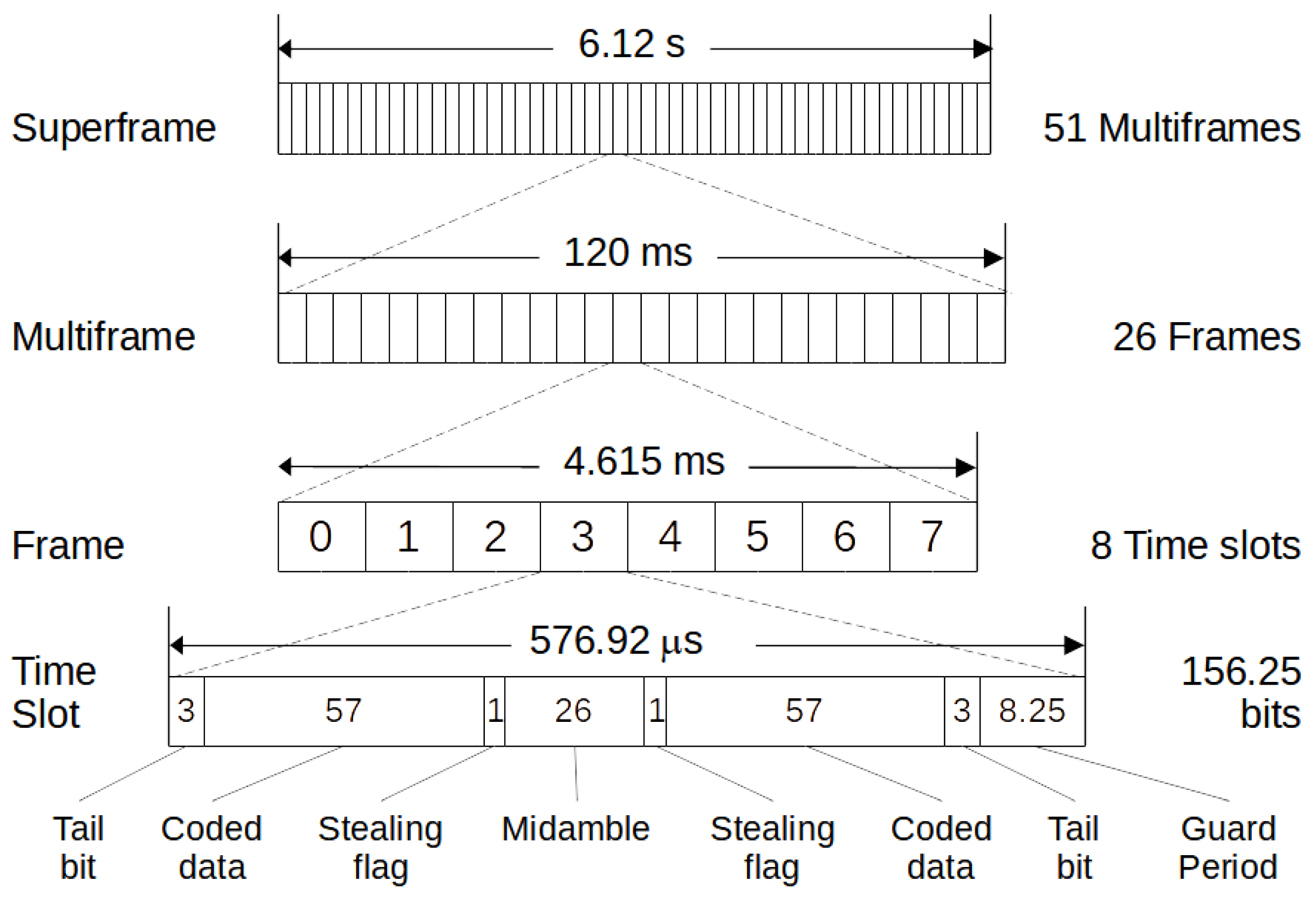
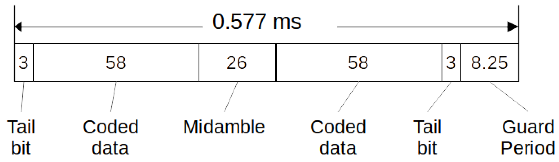
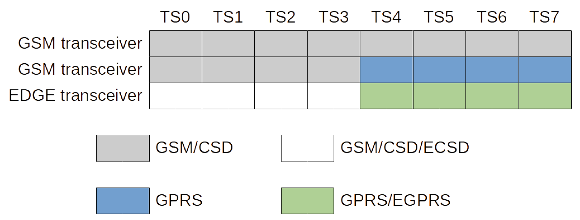
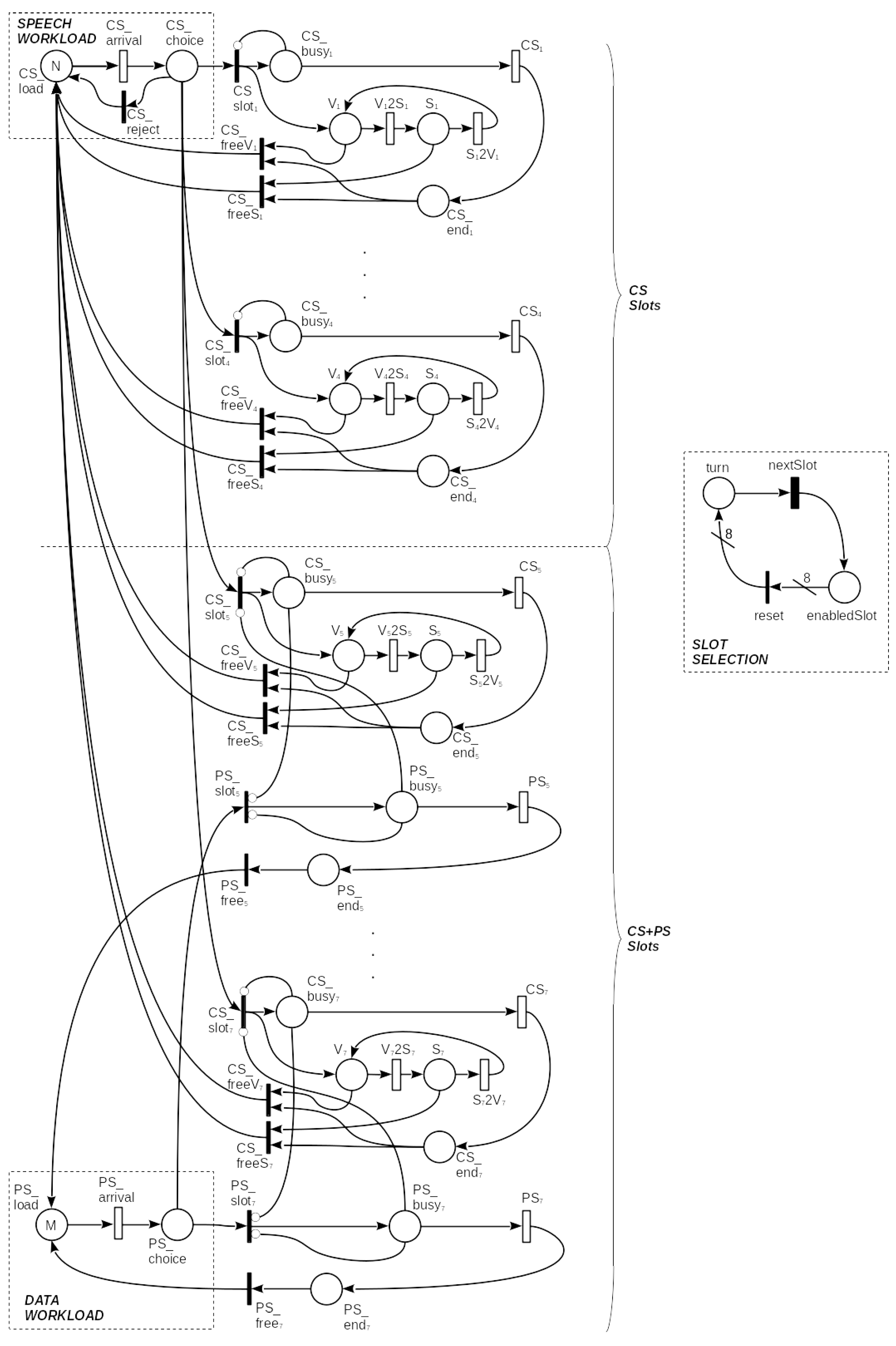
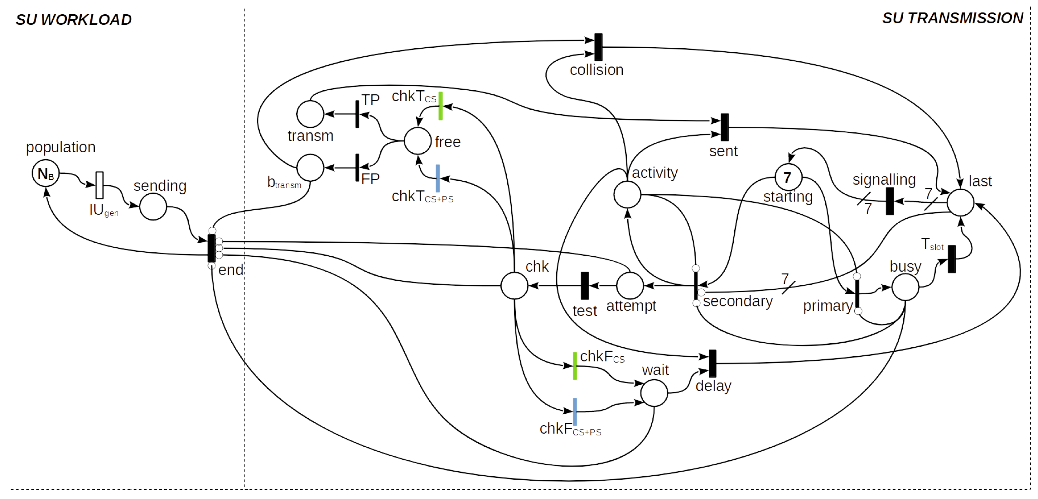
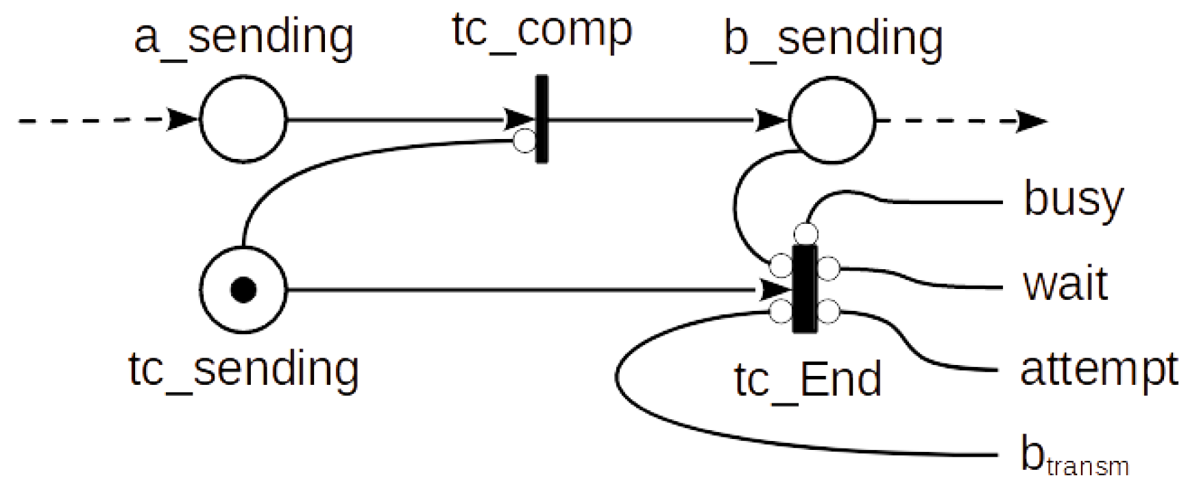
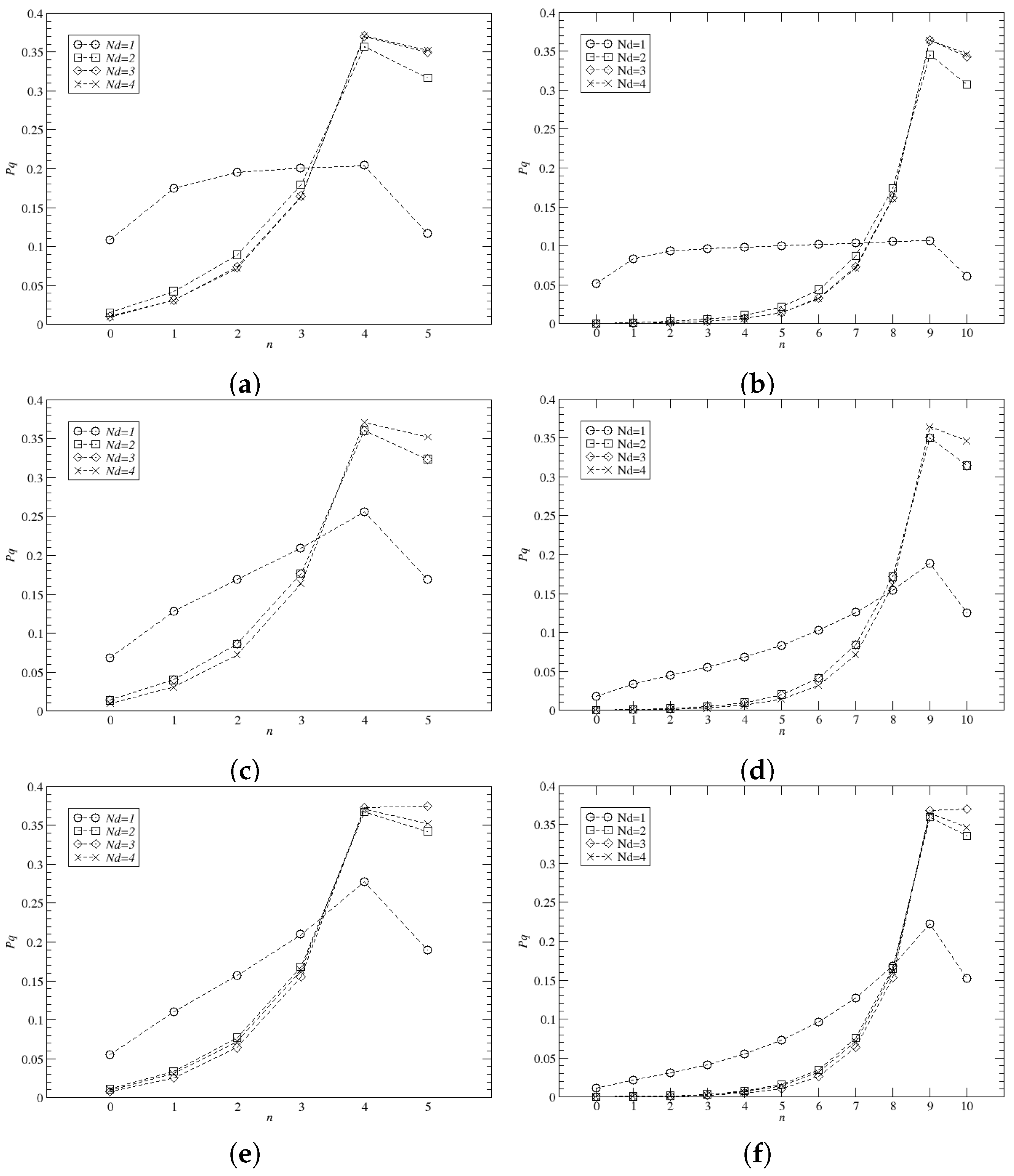
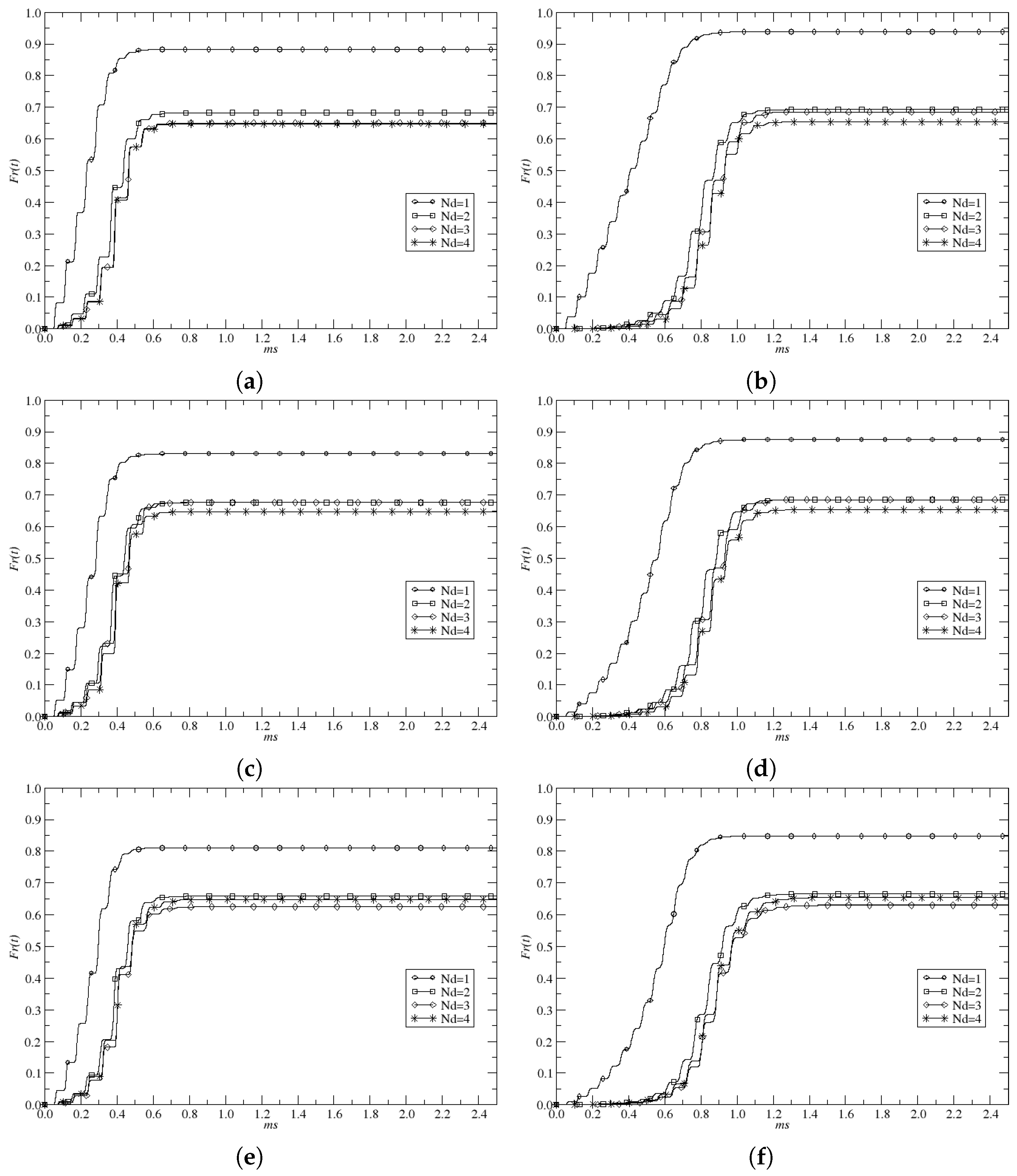
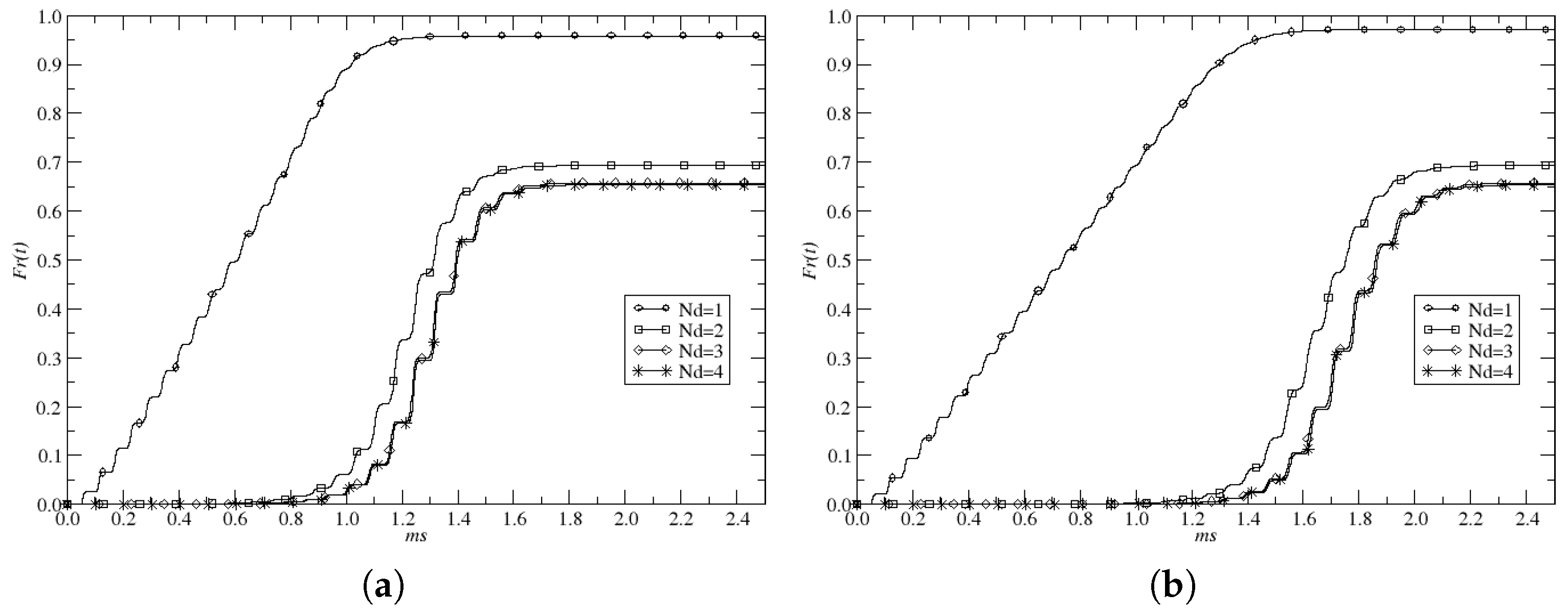
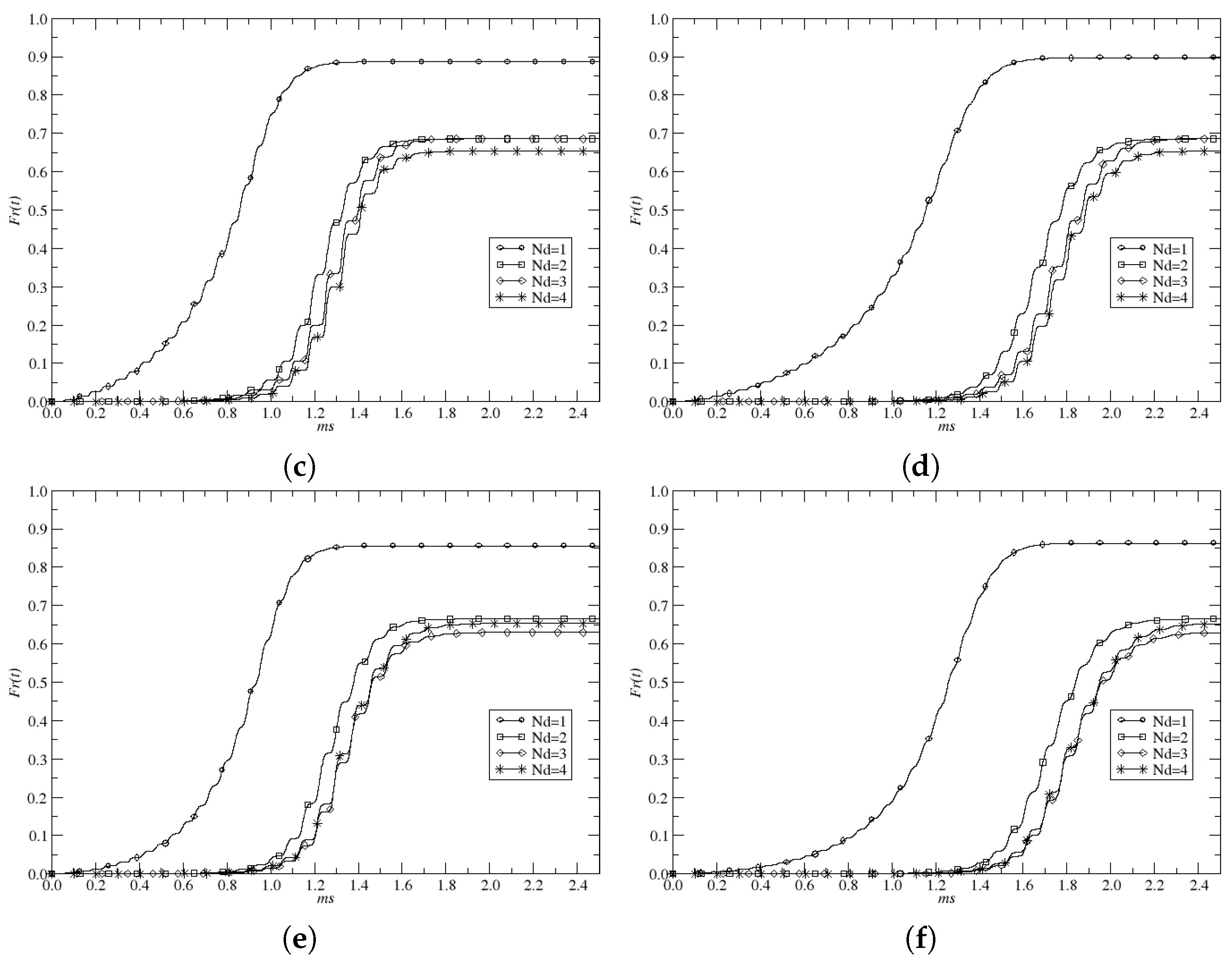
Table 1.
GSM frequency bands.
| Operating Band | Uplink Frequencies | Downlink Frequencies |
|---|---|---|
| GSM450 | 450.4–457.6 MHz | 460.4–467.6 MHz |
| GSM480 | 478.8–486.0 MHz | 488.8–496.0 MHz |
| GSM850 | 824.0–849.0 MHz | 869.0–894.0 MHz |
| GSM900 (primary) | 890.0–915.0 MHz | 935.0–960.0 MHz |
| GSM900 (extended) | 880.0–915.0 MHz | 925.0–960.0 MHz |
| GSM900 (railways) | 876.0–915.0 MHz | 921.0–960.0 MHz |
| DCS1800 | 1710.0–1785.0 MHz | 1805.0–1880.0 MHz |
| PCS1900 | 1850.0–1910.0 MHz | 1930.0–1990.0 MHz |
Table 2.
Enabling functions used in the NMSPN models.
| Model | Transition | Enabling Function |
|---|---|---|
| PU model | CSsloti | |
| CSi | ||
| Vi2Si | ||
| Si2Vi | ||
| SU model | primary | |
| secondary | ||
| chkTCS | ||
| chkFCS | ||
| chkTCS+PS | ||
| chkFCS+PS |
Table 3.
Probability to find a CS slot free ().
| 1 | 2 | 3 | 4 | ||
|---|---|---|---|---|---|
| 0.3 | 0.993 | 0.993 | 0.993 | 0.993 | |
| 1.0 | 0.977 | 0.977 | 0.977 | 0.977 | |
| 3.0 | 0.933 | 0.933 | 0.933 | 0.933 | |
Table 4.
Probability to find a CS+PS slot free ().
| 1 | 2 | 3 | 4 | ||
|---|---|---|---|---|---|
| 0.3 | 0.399 | 0.0627 | 0.00418 | 0.000268 | |
| 1.0 | 0.392 | 0.0618 | 0.00414 | 0.000267 | |
| 3.0 | 0.374 | 0.0596 | 0.00403 | 0.000263 | |
Table 5.
Loss probability.
| QS = 5 | |||||
| 1 | 2 | 3 | 4 | ||
| 0.30 | 0.117 | 0.317 | 0.350 | 0.352 | |
| 1.00 | 0.170 | 0.324 | 0.324 | 0.352 | |
| 3.00 | 0.190 | 0.342 | 0.375 | 0.352 | |
| QS = 10 | |||||
| 1 | 2 | 3 | 4 | ||
| 0.30 | 0.061 | 0.307 | 0.343 | 0.346 | |
| 1.00 | 0.125 | 0.314 | 0.314 | 0.346 | |
| 3.00 | 0.152 | 0.335 | 0.370 | 0.346 | |
| QS = 15 | |||||
| 1 | 2 | 3 | 4 | ||
| 0.30 | 0.042 | 0.307 | 0.343 | 0.346 | |
| 1.00 | 0.113 | 0.314 | 0.314 | 0.346 | |
| 3.00 | 0.144 | 0.335 | 0.370 | 0.346 | |
| QS = 20 | |||||
| 1 | 2 | 3 | 4 | ||
| 0.30 | 0.029 | 0.307 | 0.343 | 0.346 | |
| 1.00 | 0.103 | 0.314 | 0.314 | 0.346 | |
| 3.00 | 0.137 | 0.335 | 0.370 | 0.346 | |
Table 6.
Average throughput (bit/s).
| QS = 5 | |||||
| 1 | 2 | 3 | 4 | ||
| 0.30 | 40,993 | 33,162 | 32,564 | 32,487 | |
| 1.00 | 40,070 | 33,105 | 31,801 | 32,389 | |
| 3.00 | 39,392 | 32,721 | 32,238 | 31,404 | |
| QS = 10 | |||||
| 1 | 2 | 3 | 4 | ||
| 0.30 | 21,716 | 15,204 | 14,968 | 14,977 | |
| 1.00 | 19,080 | 15,162 | 14,463 | 14,866 | |
| 3.00 | 18,150 | 15,030 | 14,877 | 14,418 | |
| QS = 15 | |||||
| 1 | 2 | 3 | 4 | ||
| 0.30 | 14,811 | 9773 | 9669 | 9680 | |
| 1.00 | 11,986 | 9754 | 9284 | 9597 | |
| 3.00 | 11,300 | 9696 | 9634 | 9308 | |
| QS = 20 | |||||
| 1 | 2 | 3 | 4 | ||
| 0.30 | 11,621 | 7198 | 7140 | 7150 | |
| 1.00 | 8715 | 7186 | 6833 | 7084 | |
| 3.00 | 8162 | 7155 | 7123 | 6871 | |
Table 7.
Mean delay (ms).
| QS = 5 | |||||
| 1 | 2 | 3 | 4 | ||
| 0.30 | 0.200 | 0.247 | 0.252 | 0.252 | |
| 1.00 | 0.204 | 0.247 | 0.258 | 0.253 | |
| 3.00 | 0.208 | 0.250 | 0.254 | 0.261 | |
| QS = 10 | |||||
| 1 | 2 | 3 | 4 | ||
| 0.30 | 0.377 | 0.539 | 0.547 | 0.547 | |
| 1.00 | 0.429 | 0.540 | 0.566 | 0.551 | |
| 3.00 | 0.451 | 0.545 | 0.551 | 0.568 | |
| QS = 15 | |||||
| 1 | 2 | 3 | 4 | ||
| 0.30 | 0.553 | 0.838 | 0.847 | 0.846 | |
| 1.00 | 0.683 | 0.840 | 0.882 | 0.854 | |
| 3.00 | 0.725 | 0.845 | 0.850 | 0.880 | |
| QS = 20 | |||||
| 1 | 2 | 3 | 4 | ||
| 0.30 | 0.705 | 1.138 | 1.147 | 1.146 | |
| 1.00 | 0.940 | 1.140 | 1.199 | 1.156 | |
| 3.00 | 1.004 | 1.145 | 1.150 | 1.192 | |
Table 8.
Jitter (ms).
| QS = 5 | |||||
| 1 | 2 | 3 | 4 | ||
| 0.30 | 0.010 | 0.017 | 0.019 | 0.020 | |
| 1.00 | 0.010 | 0.017 | 0.019 | 0.020 | |
| 3.00 | 0.010 | 0.019 | 0.022 | 0.022 | |
| QS = 10 | |||||
| 1 | 2 | 3 | 4 | ||
| 0.30 | 0.037 | 0.055 | 0.067 | 0.068 | |
| 1.00 | 0.033 | 0.057 | 0.063 | 0.069 | |
| 3.00 | 0.032 | 0.065 | 0.080 | 0.075 | |
| QS = 15 | |||||
| 1 | 2 | 3 | 4 | ||
| 0.30 | 0.082 | 0.115 | 0.146 | 0.149 | |
| 1.00 | 0.063 | 0.121 | 0.133 | 0.151 | |
| 3.00 | 0.058 | 0.139 | 0.175 | 0.163 | |
| QS = 20 | |||||
| 1 | 2 | 3 | 4 | ||
| 0.30 | 0.145 | 0.199 | 0.256 | 0.261 | |
| 1.00 | 0.102 | 0.210 | 0.231 | 0.266 | |
| 3.00 | 0.089 | 0.243 | 0.310 | 0.286 | |
Disclaimer/Publisher’s Note: The statements, opinions and data contained in all publications are solely those of the individual author(s) and contributor(s) and not of MDPI and/or the editor(s). MDPI and/or the editor(s) disclaim responsibility for any injury to people or property resulting from any ideas, methods, instructions or products referred to in the content. |
© 2023 by the authors. Licensee MDPI, Basel, Switzerland. This article is an open access article distributed under the terms and conditions of the Creative Commons Attribution (CC BY) license (https://creativecommons.org/licenses/by/4.0/).
Share and Cite
MDPI and ACS Style
Serrano, S.; Scarpa, M. A Petri Net Model for Cognitive Radio Internet of Things Networks Exploiting GSM Bands. Future Internet 2023, 15, 115. https://doi.org/10.3390/fi15030115
AMA Style
Serrano S, Scarpa M. A Petri Net Model for Cognitive Radio Internet of Things Networks Exploiting GSM Bands. Future Internet. 2023; 15(3):115. https://doi.org/10.3390/fi15030115
Chicago/Turabian StyleSerrano, Salvatore, and Marco Scarpa. 2023. "A Petri Net Model for Cognitive Radio Internet of Things Networks Exploiting GSM Bands" Future Internet 15, no. 3: 115. https://doi.org/10.3390/fi15030115
Note that from the first issue of 2016, this journal uses article numbers instead of page numbers. See further details here.