
Drug Shelf Life and Release Limits Estimation Based on Manufacturing Process Capability

Abstract
:1. Introduction
2. Materials and Methods
2.1. Insulin HPLC Determination
2.1.1. Analysis of Samples
2.1.2. Long-Term Stability Study
2.2. Process Capacity Indices
2.3. Stability Data Analysis
3. Results and Discussion
3.1. HPLC Validation and Uncertainty Determination
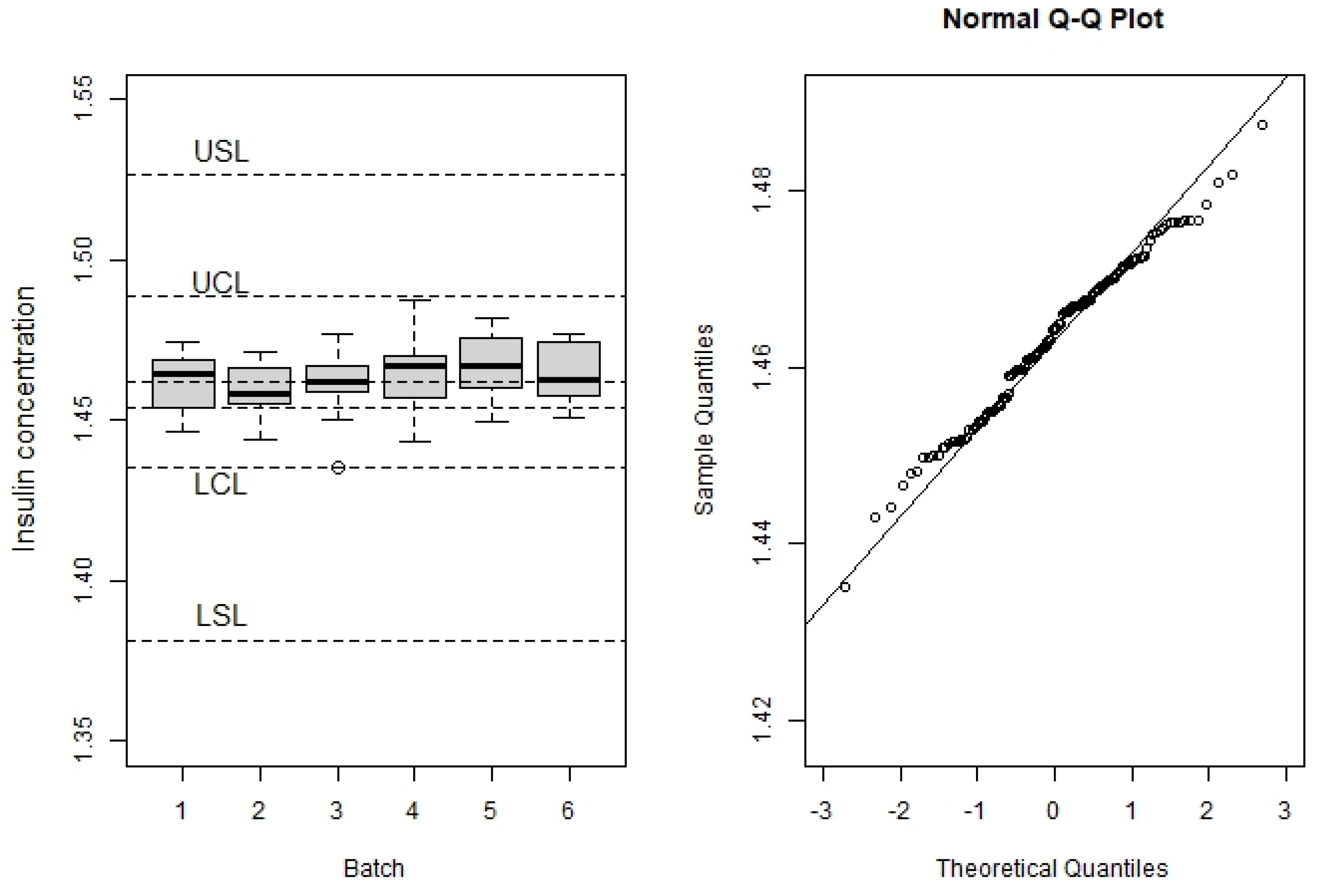
3.2. Process Capability
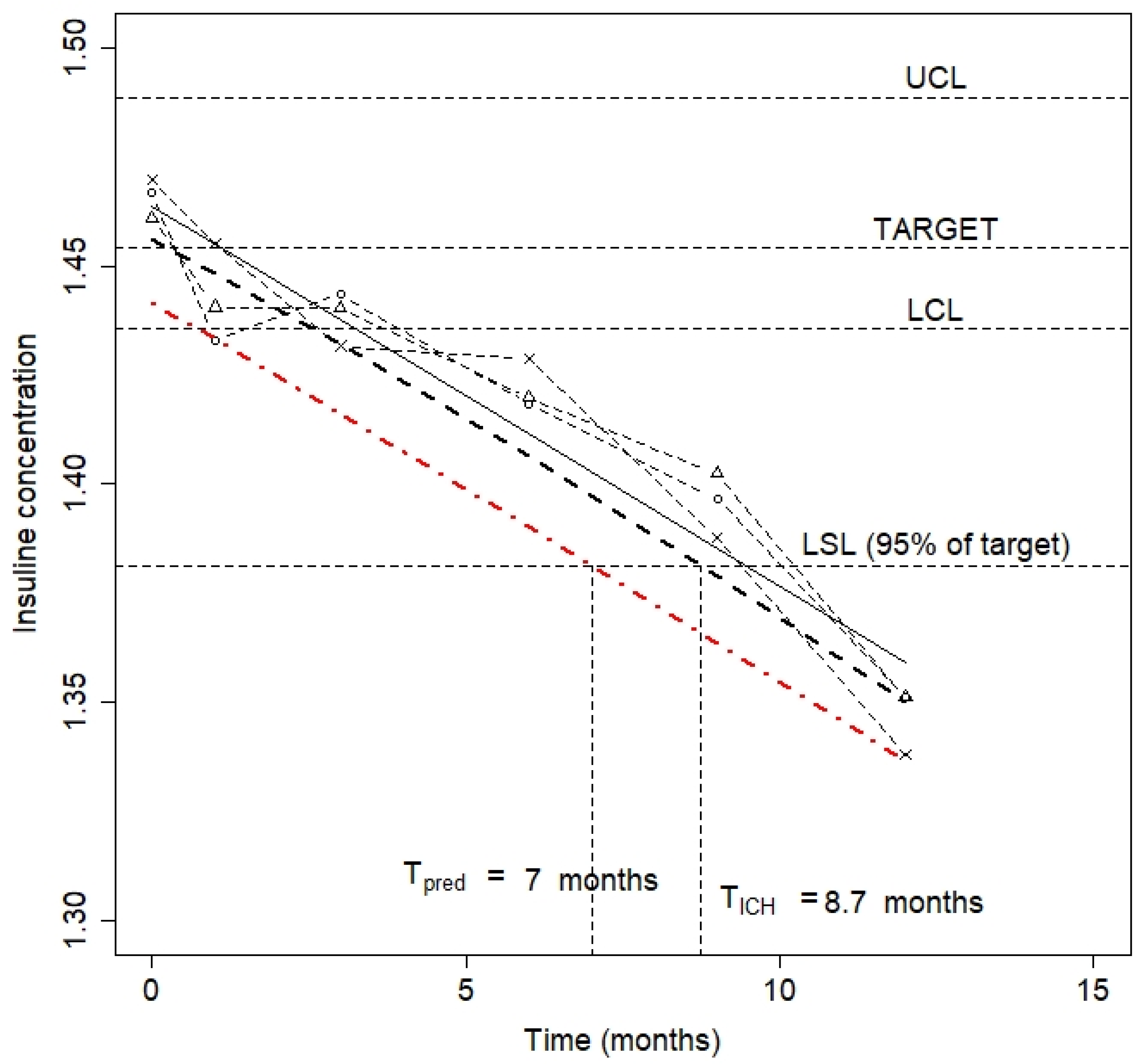
3.3. Stability
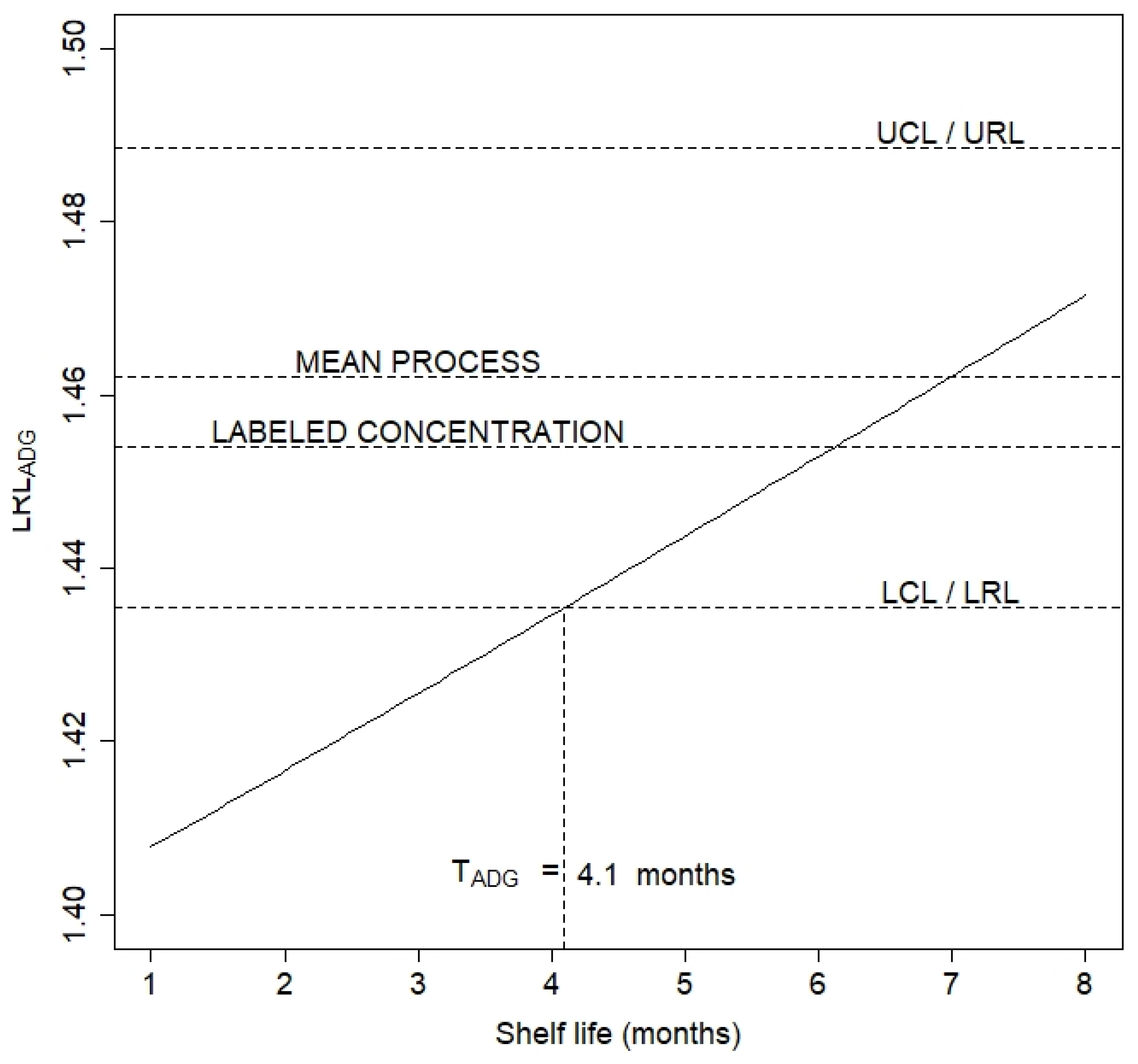
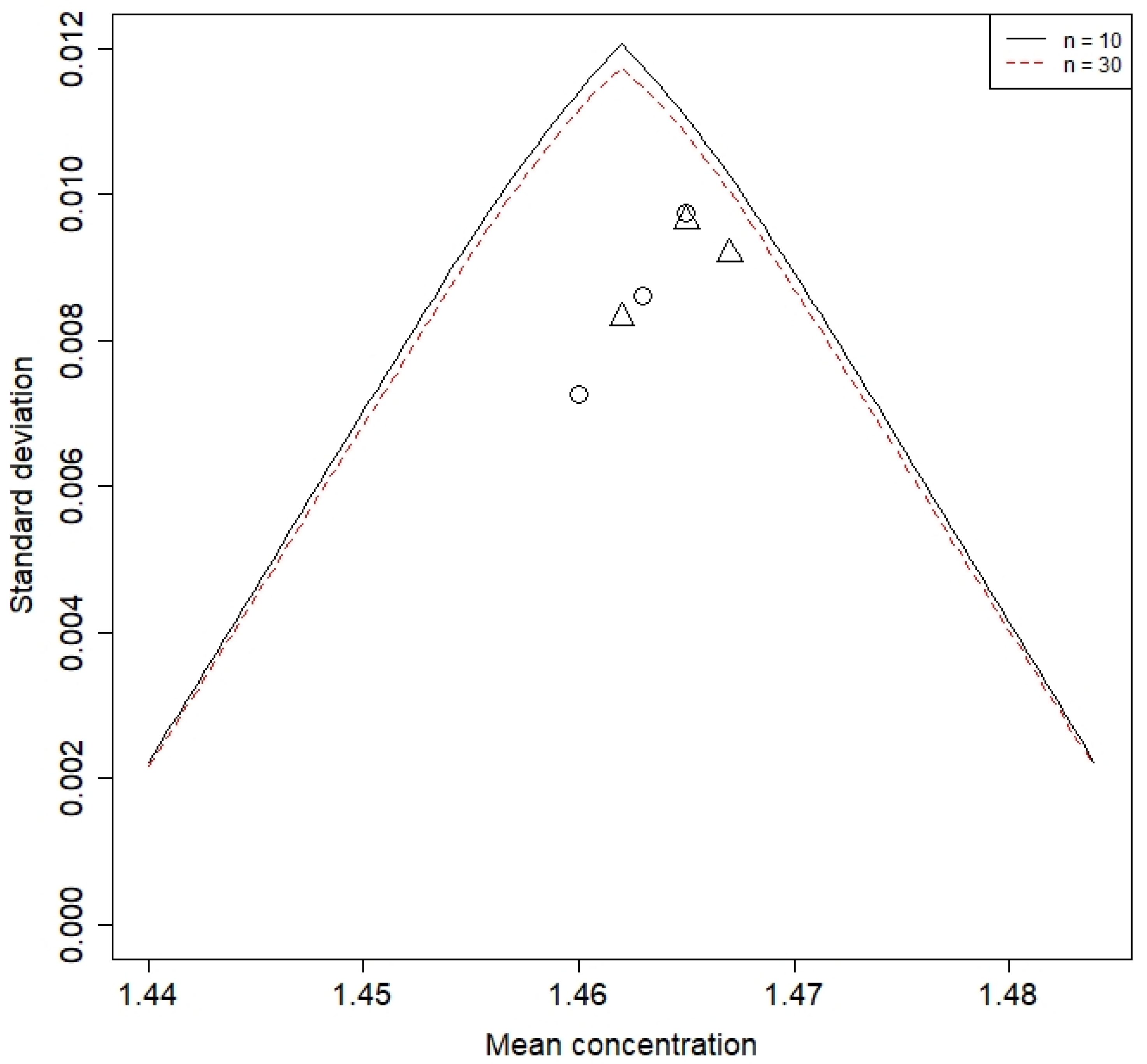
3.4. Release Limits
4. Conclusions
Supplementary Materials
Author Contributions
Funding
Institutional Review Board Statement
Informed Consent Statement
Data Availability Statement
Acknowledgments
Conflicts of Interest
References
- International Conference on Harmonization (ICH) of Technical Requirements for the Registration of Pharmaceuticals for Human Use. (ICH-Q1E) Evaluation of Stability Data. 2004.
- Murphy, J.R.; Hofer, D. Establishing shelf life, expiry limits and release limits. Drug Inf. J. 2002, 36, 769–781. [Google Scholar] [CrossRef]
- Yu, L.X.; Amidon, G.; Khan, M.A.; Hoag, S.W.; Polli, J.; Raju, G.K.; Woodcock, J. Understanding pharmaceutical quality by design. APPS J. 2014, 16, 771–783. [Google Scholar] [CrossRef] [Green Version]
- U.S. Food and Drug Administration. Guidance for Industry: Q8 (2) Pharmaceutical Development; FDA: Silver Spring, MD, USA, 2009.
- Chen, J.; Zhong, J.; Nie, L. Bayesian hierarchical modeling of drug stability data. Stat. Med. 2008, 27, 2361–2380. [Google Scholar] [CrossRef] [PubMed]
- Allen, P.V.; Dukes, G.R.; Gerger, M.E. Determination of release limits: A general methodology. Pharm. Res. 1991, 8, 1210–1213. [Google Scholar] [CrossRef] [PubMed]
- Chen, X.G.; van der Vaart, A.W. Setting the control limit at release for stability assurance. Pharm. Stat. 2022, 22, 45–63. [Google Scholar] [CrossRef] [PubMed]
- Montes, R.O.; Burdick, R.K.; Leblond, D.J. Simple approach to calculate random effects model tolerance intervals to set release and shelf-life specification limits of pharmaceutical products. J. Pharm. Sci. Technol. 2019, 73, 39–54. [Google Scholar] [CrossRef] [PubMed]
- Wei, G.C. Simple method for determination of the release limits from drug products. J. Biopharm. Stat. 1998, 8, 103–114.10. [Google Scholar] [CrossRef] [PubMed]
- Shao, J.; Chow, S.C. Constructing Release Targets for Drug Products: A Bayesian Decision Theory Approach. J. R. Stat. Ser. C Appl. Stat. 1991, 40, 381–390. [Google Scholar] [CrossRef]
- Manola, A. Assessing Release Limits and Manufacturing Risk from a Bayesian Perspective. Presented at the 2012 Midwest Biopharmaceutical Statistics Workshop, Muncie. Available online: http://www.mbswonline.com/upload/presentation_5-25-2012-10-45-1.ppt (accessed on 12 March 2023).
- Hartvig, N.V. Setting Release Limits, A Comparison of Frequentist and Bayesian Approaches. Presented at the 2016 Midwest Biopharmaceutical Statistics Workshop, Muncie. Available online: http://www.mbswonline.com/upload/presentation_7-28-2016-16-3-42.setting%20release%20limits%20nvha.pptx (accessed on 12 March 2023).
- Yu, B.; Zeng, L.; Yang, H. A Bayesian Approach to Setting the Release Limits for Critical Quality. Stat. Biopharm. Res. 2018, 10, 158–165. [Google Scholar] [CrossRef]
- Oliva, A.; Fariña, J.; Llabrés, M. Development of two high-performance liquid chromatography methods for the analysis and characterization of insulin and its derivatives in pharmaceutical preparations. J. Chromatogr. B 2000, 749, 25–34. [Google Scholar] [CrossRef] [PubMed]
- Oliva, A.; Fariña, J.; Llabrés, M. Comparison of shelf-life estimates from a human insulin pharmaceutical preparation using the matrix and full-testing approaches. Drug Dev. Ind. Pharm. 2003, 29, 513–521. [Google Scholar] [CrossRef] [PubMed]
- International Conference on Harmonization (ICH) of Technical Requirements for the Registration of Pharmaceuticals for Human Use. ICH-Q1A(R2). Stability Testing of New Drug Substances and Products. 2003. Available online: https://www.ema.europa.eu/en/documents/scientific-guideline/ich-q-1-r2-stability-testing-new-drug-substances-products-step-5_en.pdf (accessed on 10 December 2022).
- Wu, C.W.; Pearn, W.L.; Kotz, S. An overview of theory and practice on process capability indices for quality assurance. Int. J. Prod. Econ. 2009, 117, 338–359. [Google Scholar] [CrossRef]
- Boyles, R.A. The Taguchi capability index. J. Qual. Technol. 1991, 23, 17–26. [Google Scholar] [CrossRef]
- Scholz, F.; Vangel, M. Tolerance bounds and Cpk confidence bounds under batch effects. In Advances in Stochastic Models for Reliability, Quality and Safety; Kahle, W., von Collanim, E., Franz, J., Jensen, U., Eds.; Birkäuser: Boston, MA, USA, 1998; pp. 361–379. [Google Scholar]
- Pinheiro, J. nlme: Linear and Nonlinear Mixed Effects Models. Available online: https://CRAN.Rproject.org/package=nlme (accessed on 20 January 2023).
- Loy, A.; Steele, S.; Korobova, J. lmersampler: Bootstrap Method for Nested Linear Mixed-Effects Models. Available online: https://CRAN.R-project.org/package=lmeresampler (accessed on 20 January 2023).
- Fox, J.; Weisberg, S. An R Companion to Applied Regression, 3rd ed.; Sage: Thousand Oaks, CA, USA, 2019; Available online: https://socialsciences.mcmaster.ca/jfox/Books/Companion/ (accessed on 20 January 2023).
- Ruberg, S.J.; Stegeman, J.W. Pooling data for stability studies: Testing the equality of batch degradation slopes. Biometrics 1991, 47, 1059–1069. [Google Scholar] [CrossRef] [PubMed]
- Pearn, W.L.; Lin, P.C. Testing process performance based on capability index Cpk with critical values. Comput. Ind. Eng. 2004, 47, 351–369. [Google Scholar] [CrossRef]
- Wu, C.-W.; Aslam, M.; Jun, C.-H. Variables sampling inspection scheme for resubmitted lots based on the process capability index Cpk. Eur. J. Oper. Res. 2012, 217, 560–566. [Google Scholar] [CrossRef]
- Oliva, A.; Llabrés, M. Combining capability indices and control charts in the process and analytical method control strategy. In Quality Control. Intelligent Manufacturing, Robust Design and Charts; Li, P., Rodrigues Pereira, P.A., Navas, H., Eds.; IntechOpen: London, UK, 2021. [Google Scholar]
- Bordigon, S.; Scagliarini, M. Statistical analysis of process capability indices with measurement errors. Qual. Reliab. Eng. Int. 2022, 18, 321–332. [Google Scholar] [CrossRef] [Green Version]
- Duralliu, A.; Matejtschuk, P.; Stickings, P.; Hassall, L.; Tierney, R.; Williams, D.R. The influence of moisture content and temperature on the long-term storage stability of freeze-dried high concentration Immunoglobulin G (IgG). Pharmaceutics 2020, 12, 303. [Google Scholar] [CrossRef] [PubMed] [Green Version]
- Howard, J.P. Computational Methods for Numerical Analysis with R; Chapman and Hall/CRC: New York, NY, USA, 2017. [Google Scholar]
- ASTM. Standard Practice for Demonstrating Capability to Comply with an Acceptance Procedure. Designation: E2709-12; ASTM: West Conshohocken, PA, USA, 2012. [Google Scholar]


| Sigma Level | Cpk | Lower | Upper |
|---|---|---|---|
| 3 | 1.00 | 2.700 × 10⁻³ | 1.350 × 10⁻³ |
| 4 | 1.33 | 6.607 × 10⁻⁵ | 3.304 × 10⁻⁵ |
| 5 | 1.66 | 6.358 × 10⁻⁷ | 3.179 × 10⁻⁷ |
| 6 | 2.00 | 1.973 × 10⁻⁹ | 9.866 × 10⁻¹⁰ |
| Group 1 | n | min | max | mean | sd | Cpk |
|---|---|---|---|---|---|---|
| #1 | 22 | 1.447 | 1.474 | 1.463 | 8.602 × 10⁻³ | 2.49 |
| #2 | 22 | 1.444 | 1.471 | 1.460 | 7.256 × 10⁻³ | 3.07 |
| #4 | 28 | 1.443 | 1.488 | 1.465 | 9.757 × 10⁻³ | 2.12 |
| Group 2 | ||||||
| #3 | 34 | 1.435 | 1.477 | 1.462 | 8.311 × 10⁻³ | 2.61 |
| #5 | 30 | 1.450 | 1.482 | 1.467 | 9.193 × 10⁻³ | 2.17 |
| #6 | 8 | 1.451 | 1.477 | 1.465 | 9.639 × 10⁻³ | 2.14 |
| Parameter | Lower | Estimate | Upper |
|---|---|---|---|
| Intercept | 1.4597 | 1.4625 | 1.4652 |
| Batch sd | 1.80 × 10⁻⁴ | 1.59 × 10⁻³ | 1.41 × 10⁻² |
| Residual sd | 7.37 × 10⁻³ | 8.70 × 10⁻³ | 1.03 × 10⁻² |
| Batch | b0 | b1 | RSD | TICH |
|---|---|---|---|---|
| 1 | 1.461 | −8.204 × 10⁻³ | 1.360 × 10⁻² | 7.95 |
| 2 | 1.460 | −7.939 × 10⁻³ | 1.210 × 10⁻² | 8.30 |
| 4 | 1.470 | −9.980 × 10⁻³ | 1.275 × 10⁻² | 7.61 |
| Poolability | 1.464 | −8.708 × 10⁻³ | 1.186 × 10⁻² | 8.73 |
| Source of Variation | Sum of Square | DF | Mean Square | F | Pr (>F) |
|---|---|---|---|---|---|
| Intercept | 5.235 | 1 | 5.235 | 31808 | 0.000 |
| Times | 7.459 × 10⁻³ | 1 | 7.459 × 10⁻³ | 45.319 | 0.000 |
| Batch | 1.507 × 10⁻⁴ | 2 | 7.536 × 10⁻⁵ | 0.458 | 0.643 |
| Times × Batch | 2.730 × 10⁻⁴ | 2 | 1.365 × 10⁻⁴ | 0.829 | 0.460 |
| Residuals | 1.975 × 10⁻³ | 12 | 1.646 × 10⁻⁴ |
Disclaimer/Publisher’s Note: The statements, opinions and data contained in all publications are solely those of the individual author(s) and contributor(s) and not of MDPI and/or the editor(s). MDPI and/or the editor(s) disclaim responsibility for any injury to people or property resulting from any ideas, methods, instructions or products referred to in the content. |
© 2023 by the authors. Licensee MDPI, Basel, Switzerland. This article is an open access article distributed under the terms and conditions of the Creative Commons Attribution (CC BY) license (https://creativecommons.org/licenses/by/4.0/).
Share and Cite
Oliva, A.; Llabrés, M. Drug Shelf Life and Release Limits Estimation Based on Manufacturing Process Capability. Pharmaceutics 2023, 15, 1070. https://doi.org/10.3390/pharmaceutics15041070
Oliva A, Llabrés M. Drug Shelf Life and Release Limits Estimation Based on Manufacturing Process Capability. Pharmaceutics. 2023; 15(4):1070. https://doi.org/10.3390/pharmaceutics15041070
Chicago/Turabian StyleOliva, Alexis, and Matías Llabrés. 2023. "Drug Shelf Life and Release Limits Estimation Based on Manufacturing Process Capability" Pharmaceutics 15, no. 4: 1070. https://doi.org/10.3390/pharmaceutics15041070