
The Determinants of Forest Products Footprint: A New Fourier Cointegration Approach

Department of Economics, Faculty of Political Sciences, Canakkale Onsekiz Mart University, Canakkale 17200, Turkey
Forests 2023, 14(5), 875; https://doi.org/10.3390/f14050875
Submission received: 23 March 2023
/
Revised: 12 April 2023
/
Accepted: 23 April 2023
/
Published: 24 April 2023
(This article belongs to the Special Issue Forest Assessment, Modelling and Management in a Changing World)
Abstract
:This study aims to determine the factors that affect the forest products footprint (FPF) in Brazil during the period 1965–2018 by proposing a new cointegration test which augments the Engle-Granger cointegration test with a Fourier function (Fourier Engle-Granger) and allows multiple structural breaks in the long-run relationship. Since the results of the unit root tests show that all variables are nonstationary, we applied the Fourier Engle-Granger cointegration test and revealed that there was a long-term relationship between the forest products’ footprint, energy consumption, gross domestic product, and trade openness. Although energy consumption was found to have a decreasing effect on FPF, the remaining variables were found to have a healing effect on FPF. Policymakers in Brazil should consider shifting energy consumption to clean energy sources and sustain international trade and economic growth in the current form to consider the FPF.
1. Introduction
According to a report prepared by the United Nations, the consumption of primary wood products will increase by 37% to 3124 billion m3 by 2050 compared to 2020 [1]. In the face of this increasing demand, it is evident that the economy of Brazil, with the second largest forest area of 815 million hectares (after Russia with 496 million hectares), will be positively affected by this increase [2]. The forest industry in Brazil plays a significant role in the economy through investment, job creation, income production, and tax revenue. The sector accounts for 1.2% of the Brazilian GDP [3]. According to the Indústria Brasileira de Árvores (IBA), the sector creates approximately two million jobs, both directly and indirectly, and this number increases to three million when induced job posts are taken into account. In addition, the share of exports in this sector is 4.4 percent. Historically, most of Brazil’s forest products exports have been comprised of wood pulp, solid wood products, and paper products, which accounted for 94% of the country’s total forest exports in 2020. Brazil is currently the second largest exporter of wood pulp and is ranked 14th in terms of solid wood products [3].
The ecological footprint (EF) is an indicator which was developed by the Global Footprint Network to track human demand for ecological assets, and the forest products footprint (FPF) is one of the important components of the EF. The FPF is computed based on the annual consumption of timber, cellulose, timber products, and fuelwood by a nation. This is because the FPF is a consumption-based approach for measuring human impact on forests [4]. The FPF enables the assessment of the environmental impact of consuming products and promotes sustainable practices for their use.
The dynamics and determinants of the ecological footprint have been extensively studied in the literature. The ecological footprint (EF) has been extensively investigated over the last few years. For example, some studies consider the dynamics of EF and test whether shocks have permanent or transitory effects on EF (see Ulucak and Lin, [4]; Solarin and Bello, [5]; Yilanci, et al. [6], Eren and Alper, [7]; Bello et al. [8]; Yilanci et al., [9,10]), whereas others test the convergence hypothesis in the EF concept (see Ulucak and Apergis, [11]; Solarin, et al. [12]; Yilanci and Pata, [13]; Işık, et al. [14]; Tillaguango, et al. [15]; Yilanci et al. [16,17]; Ursavas and Yilanci, [18]; Alper et al. [19]; and Arogundade et al. [20]).
There are some studies that consider EF as an environmental degradation indicator and test the EKC hypothesis for countries for different periods. For instance, Al-Mulali et al. [21] undertook one of the first studies to examine the validity of the EKC hypothesis by using EF. They tested the EKC hypothesis in 93 countries and validated the EKC hypothesis in upper-middle- and high-income countries, but not in low- and lower-middle-income countries. Ozturk et al. [22], Ulucak and Bilgili [23], Destek et al. [24], Destek and Sarkodie [25], Altıntaş and Kassouri [26], Dogan et al. [27], and Ansari [28] are among the studies that test the EKC hypothesis. Some studies also considered the EF hypothesis when testing the pollution halo/haven hypothesis (see Balsalobre-Lorente et al. [29]; Destek and Okumus, [30]; Nathaniel et al. [31]; and Chaudhry et al. [32] among others.)
Focusing on the components of EF would help identify the environmental factors upon which human activities exert an impact, facilitating the development of policies in this regard. However, there are only a limited number of studies that consider components of EF instead of EF. It is possible to categorize the studies into two parts: those that solely examine the characteristics of a single series, and those that investigate relationships with other variables.
First, we focus on the studies that examine the dynamics of a single variable. Solarin et al. [33] examine the integration properties of the fishing grounds footprints (FGF) of 89 countries employing fractional integration techniques. The findings of the study show that most of the series are nonstationary; that is, shocks have permanent effects on most series. Kassouri [34] investigated the convergence pattern of the FGF for the countries in the Gulf of Guinea and the Congo Basin region using a nonlinear panel unit root test. These findings support the weak evidence of convergence in FGFs. Solarin [35] tested the stochastic properties of FPF in 89 countries over the 1961–2016 period by applying a panel stationarity test, which allows multiple structural changes via a Fourier function. The results suggest that the FPFs have a unit root, that is, the FPF will not return back to its original mean after a shock. Finally, Solarin et al. [36] test the persistence of shocks on the built-up land footprint (BLF) in 89 countries using fractional integration methods. These results support heterogeneity in the integration levels of the BLFs.
Karimi et al. [37] examined the determinants of FPFs in 17 Asia-Pacific countries from 2000 to 2017 using spatial econometric methods in an EKC framework. They found supportive evidence for EKC, and that some of the control variables, such as natural resource rents, urbanization, and energy intensity, have no effect on FPF, but government integrity, tax burden, business freedom, and monetary freedom indices have an increasing effect on FPF, and indices of trade freedom and investment freedom have a decreasing effect. They conclude by recommending that policymakers prioritize foreign direct investment and free trade. Farooq and Dar [38] examined the validity of the environmental Kuznets curve in India from 1975 to 2017 using FPF as an environmental degradation indicator. The findings of the study approve an N-shaped FPF-induced EKC in India. Yilanci et al. [39] considered the fishing grounds footprint and tested the validity of the EKC for China during the 1961–2017 period. They used the total fisheries production as a control variable. The results of this study support the validity of EKC. The results also show that total fisheries production has an increasing effect on FGF in the long- and short-run. Yilanci et al. [40] tested the pollution halo and EKC hypothesis in Indonesia from 1976 to 2018 using FGF. They found supportive evidence for both of the hypotheses. The turning point, which is a threshold value for people ignoring the environment and prioritizing their income, was found as 4579.51 US Dollars. In addition, fishery trade openness, which was used as a control variable in this study, was found to have a decreasing effect on FGF.
As seen in this review, there is emerging literature on the components of EF. This study is the first to contribute to the literature by examining the determinants of FPF in Brazil. To this end, energy consumption, GDP, and trade openness will be used as determinants. This study is novel in terms of the sample and variables used. A new test is proposed that models the structural change in the cointegration relationships between the relevant variables using a Fourier function, which is intended to provide a theoretical contribution to the literature.
2. Materials and Methods
This study aims to determine the factors affecting FPF in Brazil from 1965 to 2018. The selection of this period is due to the availability of FPF data. For this purpose, the following model is used:
where shows the forest products footprint per capita measured in global hectares, and was obtained from the website of the Global Footprint Network (https://data.footprintnetwork.org/, accessed on 15 February 2023). is the per capita gross domestic product constant at 2015 US dollar prices, and is trade openness, which is obtained by summing exports and imports and dividing the total by GDP, which indicates the degree to which a country’s trade is linked to the global economy. These two series were obtained from the data service of the World Bank. denotes the per capita energy consumption measured in gigajoules and was obtained from the Statistical Review of World Energy of BP. We use the series in logarithmic form for empirical purposes.
Table 1 presents the descriptive statistics of data:
The values in Table 1 show that LGDP has the maximum mean, whereas LTO has the minimum mean. LFPF has the least variation, which shows that the values of LFPF are more tightly clustered around the mean than those of the other series. LTO has the maximum standard deviation, which shows that the values of LTO are more spread out from the mean than in the remaining series. The p-values of the Jarque-Bera test indicate that LFPF and LTO are normally distributed.
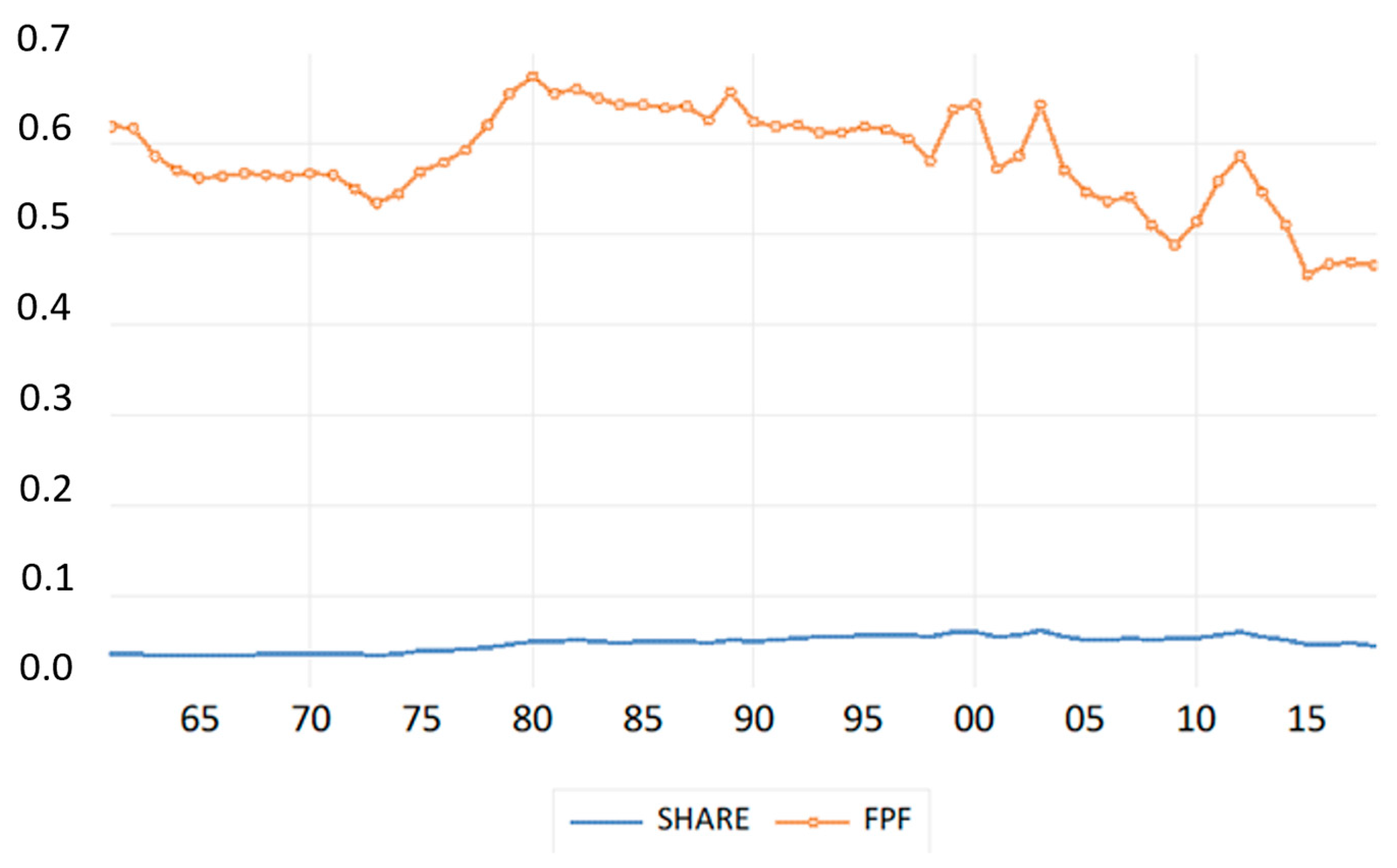
We illustrate the share of Brazil’s total FPF in the total FPF worldwide, and Brazil’s per capita FPF (global hectares) in Figure 1.
Although Brazil’s share decreased in certain years, it peaked in 2003 and started to decrease thereafter, reaching 0.045 in 2018. When evaluating the FPF per capita in Brazil, a decrease is observed until 1973, after which there was an increase up to 1980, its highest point. Thereafter, irregular increases were observed in different years, with the minimum value being recorded in 2015. Subsequently, there has been a steady uptick in its value.
3. Econometric Methodology
The performance of traditional residual-based cointegration tests that examine the null hypothesis of the no-cointegration relationship between the considered variables is affected by the structural changes that occur due to economic crises, technological changes, political regime shifts, and similar shocks. As Gregory and Hansen [41] note, if there is a structural change in the long-run relationship, the power of cointegration tests, such as Engle-Granger [42], which ignore these changes, will be reduced. Several cointegration tests have been introduced to consider structural breaks in cointegration relationships. While Gregory and Hansen [41] considered one unknown shift, Hatemi-J [43] extended this test to allow for two structural breaks. Both tests capture regime shifts by incorporating dummy variables and assume that the number of breaks is known a priori.
The study by Becker et al. ([44], BEL hereafter), who used Gallant’s [45] Flexible Fourier form to model unknown structural breaks, brought new depth to the unit root testing literature, because previous studies generally used Perron’s [46] modeling strategy of structural breaks by using dummy variables. BEL [44] showed that a single frequency of the Fourier approximation can mimic various breaks, including sharp and smooth breaks and unattended nonlinearities. Several unit root tests, such as those by BEL [44], Enders and Lee [47], and Rodrigues and Taylor [48], who employed a variant of the Flexible Fourier form, have been introduced to the literature. The main advantage of using trigonometric terms is that the locations, numbers, and forms of the structural breaks do not need to be predetermined. In this study, we extend the residual-based cointegration test of Engle-Granger [42] using Fourier approximation to test the existence of a cointegration relationship that allows unknown forms of breaks.
We consider the following cointegration regression to apply this test:
where . The dependent variable is a scalar, and is a vector of independent variables. is a deterministic function of that can be approximated using the following Fourier expansion with a single-frequency component:
where represents the traditional deterministic term, including a constant with or without a linear term, shows the number of observations, and represents the Fourier frequency, the values of which are selected using the value that minimizes the sum of squared residuals (SSR). When , there is no nonlinear trend, and the traditional Engle-Granger cointegration test emerges.
We obtain the following equation when we implement Function (2) in Model 1:
To test the null hypothesis of no cointegration, we apply the augmented Dickey–Fuller unit root test to the residuals of Model 3. Hence, we estimate the following autoregression:
where , we let show the t-statistics for the null hypothesis of no cointegration, , which is computed as:
where denotes the ordinary least squares estimator of while is the standard error of .
The critical values for the Fourier cointegration test (FEG) are obtained via simulations considering a different number of regressors (n = 1, 2, 3) and frequency values (k = 1, 2, 3, 4, 5). We report them in Table A1, considering that both constant and constant and trend cases for the sample sizes are t = 100, 500, and 1000. As shown in Table A1, the asymptotic distribution of the test statistic depends on the frequency (k) and number of regressors (n), while, ceteris paribus, an increase in k and/or n creates a decrease in critical values. We also present the finite-sample properties of the FEG test in Table A2, which shows that the test has small size distortions and good power properties in the presence of breaks.
4. Results
To apply the FEG cointegration test, the series must be integrated at one. Therefore, as a first step in the analysis, we test the integration levels of the variables using augmented Dickey-Fuller (ADF) and Zivot-Andrews (ZA) unit root tests. Table 2 presents the results of the unit root tests.
The results in Table 2 indicate that all of the series of interest have a unit root. As the variables have a unit root, we then applied the FEG cointegration test to test the long-run relationship between the variables. By using SSR, we found the optimal frequency to be 1, and the test statistic as −4.801, which is statistically significant at the 10% level. Thus, we conclude that there is long-term relationship between the variables. Next, we estimated the long-run coefficients using the fully modified ordinary least squares (FMOLS):
The results in Table 3 indicate that all regressors in the long-run model have a significant effect on the FGF.
5. Discussion
The results obtained can be evaluated from two different perspectives. The first is the unit root test, which was implemented to reveal the integration levels of the variables showing that the FGF series has a unit root; that is, the effect of a shock to these variables will be permanent; and the implemented policies would be effective and long-lasting. This finding is in line with [4], who also found the FPF to be nonstationary for the USA, and [35], who found strong evidence of a unit root in FPF for 89 nations. Second, we determined the factors that are influencing the FPF using a new Fourier cointegration test. The results indicate a long-run relationship between the FPF and energy consumption, gross domestic product, and trade openness. The long-run coefficients demonstrate that energy consumption has a detrimental effect on the FPF. A 1% increase in energy consumption causes the FGF to increase by 0.835%. For sustainable economic growth, the increase in energy consumption cannot be stopped. In 2018, renewable energy consumption and fossil fuel (oil, natural gas, and coal) shares in primary energy consumption were 19% and 53%, respectively, in Brazil (see BP [49]), indicating that an increase in energy consumption will have a detrimental effect on the environment because the share of fossil fuel consumption is higher than that of renewable energy consumption. In addition, 16.583 × 10³ tonnes of oil equivalent (TOE) was consumed in 2009 for energy use, whereas in 2018, this quantity increased by 16.758 × 10³ TOE, showing that the amount of wood used for energy consumption increased over the ten-year period. These results confirm the findings of Arouri et al. [50], Ilham [51], Chen et al. [52], Lu [53], and Adekoya et al. [54].
The coefficient of LGDP has a negative value; that is, the gross domestic product has a healing effect on FGF, that is, an increase in GDP improves the environment. This circumstance is intimately related to the Environmental Kuznets Curve. As income increases, awareness about the environment grows. Individuals demand enhanced ecological conditions, prompting governmental bodies to enforce policies and legislation aimed at mitigating contamination and facilitating a shift towards more sustainable technological advancements. As FGF is a consumption-oriented index, the healing effect of GDP indicates that consumers might lean towards recycling. A 1% increase in LGDP causes a 0.753% decrease in FGF. This result supports the findings of Chandran and Tang [55], Dogan and Turkekul [56], Osuntuyi and Lean [57], and Jahanger et al. [58].
Trade openness has a decreasing effect on LFPF. If there is a 1% increase in trade openness, the FPF decreases by 0.418% in Brazil, which suggests that trade liberalization mitigates environmental contamination by delegating manufacturing processes to foreign nations that boast eco-friendly technologies that are capable of suppressing emissions. Such a deleterious outcome conveys that the nation in question reaps the benefits of unfettered commerce, while concurrently enhancing ecological standards (see Dada et al. [59]). This result is in line with Destek and Sinha [60], who found that trade openness has a diminishing effect on the ecological footprint. These results support the findings of Liu et al. [61], Ozturk et al. [22], Khan et al. [62], and Yao et al. [63], but are contrary to the findings of Kongbuamai et al. [64], and Dada et al. [59].
6. Conclusions
This study considered a consumption-oriented environmental degradation indicator, the forest grounds footprint (FGF), and aimed to examine the determinants of the index in Brazil from the 1965 to 2018 period. The examination was conducted by proposing a new cointegration test that allowed multiple smooth breaks in the long-run relationship. Because this test was an augmentation of the traditional Engle-Granger cointegration test with a Fourier function, we called this test the Fourier Engle-Granger (FEG) cointegration test. Owing to the FEG cointegration test, we do not need to know the exact location, form or number of breaks a priori. The suggested test can prevent the potential loss of power in the cointegration tests that allow structural breaks by adding dummy variables to the testing equations. The simulation results show that the FEG test has small size distortions and good power properties, especially in the presence of breaks.
The results of the FEG cointegration test revealed a long-term relationship between the forest grounds footprint and gross domestic product (GDP), energy consumption, and trade openness (TO). The coefficients of long-run estimation show that energy consumption has an increasing effect on FGF, whereas GDP and TO have a decreasing effect on FGF. Therefore, policymakers in Brazil should consider increasing international trade to protect environmental quality. In addition, energy consumption should be diversified, and the intensity of energy consumption should be shifted to clean energy. Moreover, economic growth should be maintained through current components.
Funding
This research received no external funding.
Data Availability Statement
The data can be obtained from the databases of the Global Footprint Network, British Petroleum, and the World Bank.
Conflicts of Interest
The author declares that they have no conflict of interest.
Appendix A. Size and Power Properties
We analyzed the finite sample properties of the suggested test by considering the following data generation process (DGP):
where , and . We assume that and . Similar DGPs have been used in several prior studies [see Banerjee et al. [65], Lee et al. [66], Banerjee et al. [67], among others.]. We conducted simulations using 20,000 replications at the 5% significance level. We examined the performance of the test from different perspectives:
- -
- we let the persistent measure change in the range {0, 0.9};
- -
- we set , while letting the vary along with ; and,
- -
- we also evaluated two sets of , and as and .
We report the results in Table A1.

Table A1.
Finite Sample Performance of the FEG Cointegration Test.
| Model with a Constant | Model with a Constant and a Trend | ||||||||||
|---|---|---|---|---|---|---|---|---|---|---|---|
| T = 100 | T = 300 | T = 100 | T = 300 | ||||||||
| 0 | 1 | 0 | 0 | 0.053 | 0.233 | 0.053 | 0.761 | 0.048 | 0.101 | 0.053 | 0.609 |
| 0 | 16 | 0 | 0 | 0.052 | 0.234 | 0.051 | 0.758 | 0.051 | 0.099 | 0.049 | 0.607 |
| 0.9 | 1 | 0 | 0 | 0.045 | 0.175 | 0.039 | 0.755 | 0.049 | 0.096 | 0.045 | 0.594 |
| 0.9 | 16 | 0 | 0 | 0.046 | 0.173 | 0.038 | 0.753 | 0.050 | 0.095 | 0.043 | 0.598 |
| 0 | 1 | 3 | 0 | 0.066 | 0.214 | 0.053 | 0.816 | 0.048 | 0.097 | 0.053 | 0.646 |
| 0 | 16 | 3 | 0 | 0.066 | 0.217 | 0.051 | 0.815 | 0.051 | 0.098 | 0.049 | 0.646 |
| 0.9 | 1 | 3 | 0 | 0.060 | 0.219 | 0.039 | 0.807 | 0.049 | 0.089 | 0.045 | 0.634 |
| 0.9 | 16 | 3 | 0 | 0.059 | 0.220 | 0.038 | 0.807 | 0.050 | 0.091 | 0.043 | 0.640 |
| 0 | 1 | 0 | 5 | 0.053 | 0.677 | 0.053 | 1 | 0.048 | 0.163 | 0.053 | 1 |
| 0 | 16 | 0 | 5 | 0.052 | 0.677 | 0.051 | 1 | 0.051 | 0.164 | 0.049 | 1 |
| 0.9 | 1 | 0 | 5 | 0.045 | 0.638 | 0.039 | 1 | 0.049 | 0.166 | 0.045 | 1 |
| 0.9 | 16 | 0 | 5 | 0.046 | 0.640 | 0.038 | 1 | 0.050 | 0.172 | 0.043 | 1 |
| 0 | 1 | 3 | 5 | 0.053 | 0.517 | 0.053 | 1 | 0.048 | 0.117 | 0.053 | 1 |
| 0 | 16 | 3 | 5 | 0.052 | 0.521 | 0.051 | 1 | 0.051 | 0.117 | 0.049 | 1 |
| 0.9 | 1 | 3 | 5 | 0.045 | 0.429 | 0.039 | 1 | 0.049 | 0.105 | 0.045 | 1 |
| 0.9 | 16 | 3 | 5 | 0.046 | 0.430 | 0.038 | 1 | 0.050 | 0.109 | 0.043 | 1 |
Note: , and represents the size, and power properties, respectively.
The results show that, as the sample size increases, the power of the test also increases (the conventional Engle-Granger [42] cointegration test loses power and suffers from size distortions in the presence of breaks. The results are available from the author upon request). In addition, in the case of , when the magnitude of the break increases, the power of the FEG test increases and becomes 1 in most cases. When the persistent measure increases, the power of the test seems to decrease in the case of . In this case, an increase in causes an increase in the power of the test in most cases. Overall, the test seems to have small size distortions and good power properties with regard to the existence of breaks.
Appendix B. Critical Values
Table A2.
Critical Values of the FEG Cointegration Test.
| Model with a Constant | Model with a Constant and Trend | ||||||||||||||||||
|---|---|---|---|---|---|---|---|---|---|---|---|---|---|---|---|---|---|---|---|
| n | k | T = 100 | t = 500 | t = 1000 | T = 100 | t = 500 | t = 1000 | ||||||||||||
| 1% | 5% | 10% | 1% | 5% | 10% | 1% | 5% | 10% | 1% | 5% | 10% | 1% | 5% | 10% | 1% | 5% | 10% | ||
| 1 | 1 | −4.906 | −4.302 | −3.988 | −4.756 | −4.198 | −3.898 | −4.738 | −4.175 | −3.886 | −5.354 | −4.731 | −4.423 | −5.128 | −4.576 | −4.293 | −5.074 | −4.555 | −4.274 |
| 2 | −4.665 | −3.995 | −3.648 | −4.517 | −3.912 | −3.589 | −4.503 | −3.898 | −3.579 | −5.243 | −4.582 | −4.250 | −4.995 | −4.433 | −4.136 | −4.973 | −4.410 | −4.119 | |
| 3 | −4.437 | −3.743 | −3.380 | −4.333 | −3.685 | −3.349 | −4.314 | −3.686 | −3.342 | −5.002 | −4.340 | −3.997 | −4.801 | −4.230 | −3.910 | −4.804 | −4.208 | −3.901 | |
| 4 | −4.285 | −3.599 | −3.252 | −4.183 | −3.554 | −3.231 | −4.172 | −3.546 | −3.221 | −4.849 | −4.175 | −3.827 | −4.697 | −4.092 | −3.767 | −4.693 | −4.088 | −3.769 | |
| 5 | −4.190 | −3.520 | −3.187 | −4.091 | −3.478 | −3.165 | −4.081 | −3.477 | −3.165 | −4.774 | −4.086 | −3.739 | −4.634 | −3.997 | −3.683 | −4.593 | −3.994 | −3.677 | |
| 2 | 1 | −5.282 | −4.655 | −4.337 | −5.067 | −4.511 | −4.220 | −5.048 | −4.487 | −4.205 | −5.641 | −5.026 | −4.705 | −5.404 | −4.855 | −4.571 | −5.367 | −4.826 | −4.550 |
| 2 | −5.168 | −4.526 | −4.189 | −4.969 | −4.394 | −4.085 | −4.949 | −4.371 | −4.065 | −5.598 | −4.954 | −4.633 | −5.329 | −4.772 | −4.480 | −5.295 | −4.748 | −4.460 | |
| 3 | −4.958 | −4.283 | −3.938 | −4.804 | −4.183 | −3.870 | −4.778 | −4.172 | −3.852 | −5.450 | −4.781 | −4.436 | −5.199 | 4.620 | −4.313 | −5.167 | −4.597 | −4.292 | |
| 4 | −4.805 | −4.122 | −3.767 | −4.647 | −4.048 | −3.722 | −4.657 | −4.040 | −3.716 | −5.294 | −4.622 | −4.271 | −5.089 | −4.487 | −4.183 | −5.065 | −4.469 | −4.158 | |
| 5 | −4.708 | −4.033 | −3.689 | −4.587 | −3.964 | −3.633 | −4.536 | −3.935 | −3.629 | −5.203 | −4.508 | −4.164 | −5.006 | −4.404 | −4.086 | −4.945 | −4.370 | −4.063 | |
| 3 | 1 | −5.596 | −4.957 | −4.640 | −5.354 | −4.796 | −4.512 | −5.315 | −4.786 | −4.497 | −5.941 | −5.294 | −4.971 | −5.638 | −5.094 | −4.814 | −5.602 | −5.070 | −4.795 |
| 2 | −5.573 | −4.918 | −4.593 | −5.330 | −4.752 | −4.460 | −5.286 | −4.727 | −4.435 | −5.926 | −5.278 | −4.961 | −5.635 | −5.078 | −4.791 | −5.590 | −5.048 | −4.762 | |
| 3 | −5.393 | −4.733 | −4.394 | −5.177 | −4.597 | −4.285 | −5.150 | −4.582 | −4.277 | −5.792 | −5.141 | −4.806 | −5.515 | −4.964 | −4.659 | −5.504 | −4.940 | −4.643 | |
| 4 | −5.271 | −4.605 | −4.252 | −5.071 | −4.468 | −4.148 | −5.035 | −4.134 | −4.455 | −5.698 | −5.023 | −4.681 | −5.441 | −4.843 | −4.534 | −5.404 | −4.835 | −4.529 | |
| 5 | −5.155 | −4.478 | −4.127 | −4.976 | −4.378 | −4.056 | −4.959 | −4.352 | −4.042 | −5.601 | −4.905 | −4.560 | −5.361 | −4.752 | −4.436 | −5.332 | −4.743 | −4.435 | |
Note: n, k, and T show the number of independent variables, the number of frequencies of the Fourier function, and the sample size.
References
- FAO. Global Forest Resources Assessment 2020: Main Report; UN Food and Agriculture Organization: Rome, Italy, 2020. [Google Scholar]
- FAO. Global Forest Sector Outlook 2050: Assessing Future Demand and Sources of Timber for a Sustainable Economy—Background Paper for the State of the World’s Forests 2022; FAO Forestry Working Paper, No. 31.; UN Food and Agriculture Organization: Rome, Italy, 2022. [Google Scholar] [CrossRef]
- Arias, E. Brazil: Market Profil; The South Carolina Forestry Commission: Columbia, SC, USA, 2022.
- Ulucak, R.; Lin, D. Persistence of policy shocks to ecological footprint of the USA. Ecol. Indic. 2017, 80, 337–343. [Google Scholar] [CrossRef]
- Solarin, S.A.; Bello, M.O. Persistence of policy shocks to an environmental degradation index: The case of ecological footprint in 128 developed and developing countries. Ecol. Indic. 2018, 89, 35–44. [Google Scholar] [CrossRef]
- Yilanci, V.; Gorus, M.S.; Aydin, M. Are shocks to ecological footprint in OECD countries permanent or temporary? J. Clean. Prod. 2019, 212, 270–301. [Google Scholar] [CrossRef]
- Eren, A.E.; Alper, F.Ö. Persistence of Policy Shocks to the Ecological Footprint of MINT Countries. Ege Acad. Rev. 2021, 21, 427–440. [Google Scholar] [CrossRef]
- Bello, M.O.; Erdogan, S.; Ch’Ng, K.S. On the convergence of ecological footprint in African countries: New evidences from panel stationarity tests with factors and gradual shifts. J. Environ. Manag. 2022, 322, 116061. [Google Scholar] [CrossRef]
- Yilanci, V.; Ulucak, R.; Ozgur, O. Insights for a sustainable environment: Analysing the persistence of policy shocks to ecological footprints of Mediterranean countries. Spat. Econ. Anal. 2022, 17, 47–66. [Google Scholar] [CrossRef]
- Yilanci, V.; Pata, U.K.; Cutcu, I. Testing the persistence of shocks on ecological footprint and sub-accounts: Evidence from the big ten emerging markets. Int. J. Environ. Res. 2022, 16, 10. [Google Scholar] [CrossRef]
- Ulucak, R.; Apergis, N. Does convergence really matter for the environment? An application based on club convergence and on the ecological footprint concept for the EU countries. Environ. Sci. Policy 2018, 80, 21–27. [Google Scholar] [CrossRef]
- Solarin, S.A.; Tiwari, A.K.; Bello, M.O. A multi-country convergence analysis of ecological footprint and its components. Sustain. Cities Soc. 2019, 46, 101422. [Google Scholar] [CrossRef]
- Yilanci, V.; Pata, U.K. Convergence of per capita ecological footprint among the ASEAN-5 countries: Evidence from a non-linear panel unit root test. Ecol. Indic. 2020, 113, 106178. [Google Scholar] [CrossRef]
- Işık, C.; Ahmad, M.; Ongan, S.; Ozdemir, D.; Irfan, M.; Alvarado, R. Convergence analysis of the ecological footprint: Theory and empirical evidence from the USMCA countries. Environ. Sci. Pollut. Res. 2021, 28, 32648–32659. [Google Scholar] [CrossRef]
- Tillaguango, B.; Alvarado, R.; Dagar, V.; Murshed, M.; Pinzón, Y.; Méndez, P. Convergence of the ecological footprint in Latin America: The role of the productive structure. Environ. Sci. Pollut. Res. 2021, 28, 59771–59783. [Google Scholar] [CrossRef] [PubMed]
- Yilanci, V.; Gorus, M.S.; Solarin, S.A. Convergence in per capita carbon footprint and ecological footprint for G7 countries: Evidence from panel Fourier threshold unit root test. Energy Environ. 2022, 33, 527–545. [Google Scholar] [CrossRef]
- Yilanci, V.; Ursavaş, U.; Ursavaş, N. Convergence in ecological footprint across the member states of ECOWAS: Evidence from a novel panel unit root test. Environ. Sci. Pollut. Res. 2022, 29, 79241–79252. [Google Scholar] [CrossRef] [PubMed]
- Ursavaş, U.; Yilanci, V. Convergence analysis of ecological footprint at different time scales: Evidence from Southern Common Market countries. Energy Environ. 2023, 34, 429–442. [Google Scholar] [CrossRef]
- Alper, A.E.; Alper, F.O.; Cil, A.B.; Iscan, E.; Eren, A.A. Stochastic convergence of ecological footprint: New insights from a unit root test based on smooth transitions and nonlinear adjustment. Environ. Sci. Pollut. Res. 2023, 30, 22100–22114. [Google Scholar] [CrossRef]
- Arogundade, S.; Hassan, A.; Akpa, E.; Mduduzi, B. Closer together or farther apart: Are there club convergence in ecological footprint? Environ. Sci. Pollut. Res. 2023, 30, 15293–15310. [Google Scholar] [CrossRef]
- Al-Mulali, U.; Weng-Wai, C.; Sheau-Ting, L.; Mohammed, A.H. Investigating the environmental Kuznets curve (EKC) hypothesis by utilizing the ecological footprint as an indicator of environmental degradation. Ecol. Indic. 2015, 48, 315–323. [Google Scholar] [CrossRef]
- Ozturk, I.; Al-Mulali, U.; Saboori, B. Investigating the environmental Kuznets curve hypothesis: The role of tourism and ecological footprint. Environ. Sci. Pollut. Res. 2016, 23, 1916–1928. [Google Scholar] [CrossRef]
- Ulucak, R.; Bilgili, F. A reinvestigation of EKC model by ecological footprint measurement for high, middle and low income countries. J. Clean. Prod. 2018, 188, 144–157. [Google Scholar] [CrossRef]
- Destek, M.A.; Ulucak, R.; Dogan, E. Analyzing the environmental Kuznets curve for the EU countries: The role of ecological footprint. Environ. Sci. Pollut. Res. 2018, 25, 29387–29396. [Google Scholar] [CrossRef] [PubMed]
- Destek, M.A.; Sarkodie, S.A. Investigation of environmental Kuznets curve for ecological footprint: The role of energy and financial development. Sci. Total Environ. 2019, 650, 2483–2489. [Google Scholar] [CrossRef] [PubMed]
- Altıntaş, H.; Kassouri, Y. Is the environmental Kuznets Curve in Europe related to the per-capita ecological footprint or CO2 emissions? Ecol. Indic. 2020, 113, 106187. [Google Scholar] [CrossRef]
- Dogan, E.; Ulucak, R.; Kocak, E.; Isik, C. The use of ecological footprint in estimating the environmental Kuznets curve hypothesis for BRICST by considering cross-section dependence and heterogeneity. Sci. Total Environ. 2020, 723, 138063. [Google Scholar] [CrossRef]
- Ansari, M.A. Re-visiting the Environmental Kuznets curve for ASEAN: A comparison between ecological footprint and carbon dioxide emissions. Renew. Sustain. Energy Rev. 2022, 168, 112867. [Google Scholar] [CrossRef]
- Balsalobre-Lorente, D.; Gokmenoglu, K.K.; Taspinar, N.; Cantos-Cantos, J.M. An approach to the pollution haven and pollution halo hypotheses in MINT countries. Environ. Sci. Pollut. Res. 2019, 26, 23010–23026. [Google Scholar] [CrossRef]
- Destek, M.A.; Okumus, I. Does pollution haven hypothesis hold in newly industrialized countries? Evidence from ecological footprint. Environ. Sci. Pollut. Res. 2019, 26, 23689–23695. [Google Scholar] [CrossRef]
- Nathaniel, S.; Aguegboh, E.; Iheonu, C.; Sharma, G.; Shah, M. Energy consumption, FDI, and urbanization linkage in coastal Mediterranean countries: Re-assessing the pollution haven hypothesis. Environ. Sci. Pollut. Res. 2020, 27, 35474–35487. [Google Scholar] [CrossRef]
- Chaudhry, I.S.; Yin, W.; Ali, S.A.; Faheem, M.; Abbas, Q.; Farooq, F.; Ur Rahman, S. Moderating role of institutional quality in validation of pollution haven hypothesis in BRICS: A new evidence by using DCCE approach. Environ. Sci. Pollut. Res. 2022, 29, 9193–9202. [Google Scholar] [CrossRef]
- Solarin, S.A.; Gil-Alana, L.A.; Lafuente, C. Persistence and sustainability of fishing grounds footprint: Evidence from 89 countries. Sci. Total Environ. 2021, 751, 141594. [Google Scholar] [CrossRef] [PubMed]
- Kassouri, Y. Exploring the dynamics of fishing footprints in the Gulf of Guinea and Congo Basin region: Current status and future perspectives. Mar. Policy 2021, 133, 104739. [Google Scholar] [CrossRef]
- Solarin, S.A. Towards sustainable development: A multi-country persistence analysis of forest products footprint using a stationarity test with smooth shifts. Sustain. Dev. 2020, 28, 1465–1476. [Google Scholar] [CrossRef]
- Solarin, S.A.; Gil-Alana, L.A.; Lafuente, C. Persistence and non-stationarity in the built-up land footprint across 89 countries. Ecol. Indic. 2021, 123, 107372. [Google Scholar] [CrossRef]
- Karimi, M.S.; Khezri, M.; Khan, Y.A.; Razzaghi, S. Exploring the influence of economic freedom index on fishing grounds footprint in environmental Kuznets curve framework through spatial econometrics technique: Evidence from Asia-Pacific countries. Environ. Sci. Pollut. Res. 2022, 29, 6251–6266. [Google Scholar] [CrossRef] [PubMed]
- Farooq, U.; Dar, A.B. Is there a Kuznets curve for forest product footprint?—Empirical evidence from India. For. Policy Econ. 2022, 144, 102850. [Google Scholar] [CrossRef]
- Yilanci, V.; Cutcu, I.; Cayir, B. Is the environmental Kuznets curve related to the fishing footprint? Evidence from China. Fish. Res. 2022, 254, 106392. [Google Scholar] [CrossRef]
- Yilanci, V.; Cutcu, I.; Cayir, B.; Saglam, M.S. Pollution haven or pollution halo in the fishing footprint: Evidence from Indonesia. Mar. Pollut. Bull. 2023, 188, 114626. [Google Scholar] [CrossRef]
- Gregory, A.W.; Hansen, B.E. Residual-based tests for cointegration in models with regime shifts. J. Econom. 1996, 70, 99–126. [Google Scholar] [CrossRef]
- Engle, R.; Granger, C. Co-integration and error correction: Representation, estimation, and testing. Econometrica 1987, 55, 251–276. [Google Scholar] [CrossRef]
- Hatemi-j, A. Tests for cointegration with two unknown regime shifts with an application to financial market integration. Empir. Econ. 2008, 35, 497–505. [Google Scholar] [CrossRef]
- Becker, R.; Enders, W.; Lee, J. A stationarity test in the presence of an unknown number of smooth breaks. J. Time Ser. Anal. 2006, 27, 381–409. [Google Scholar] [CrossRef]
- Gallant, R. On the basis in flexible functional form and an essentially unbiased form: The flexible Fourier form. J. Econom. 1981, 15, 211–353. [Google Scholar] [CrossRef]
- Perron, P. The great crash, the oil price shock, and the unit root hypothesis. Econometrica 1989, 57, 1361–1401. [Google Scholar] [CrossRef]
- Enders, W.; Lee, J. The flexible Fourier form and Dickey–Fuller type unit root tests. Econ. Lett. 2012, 117, 196–199. [Google Scholar] [CrossRef]
- Rodrigues, P.M.; Robert Taylor, A.M. The Flexible Fourier Form and Local Generalised Least Squares De-trended Unit Root Tests. Oxf. Bull. Econ. Stat. 2012, 74, 736–759. [Google Scholar] [CrossRef]
- BP 2022, Statistical Review of World Energy—2022, The Brazilian Energy System in 2021. 2022. Available online: https://www.bp.com/content/dam/bp/business-sites/en/global/corporate/pdfs/energy-economics/statistical-review/bp-stats-review-2022-brazil-insights.pdf (accessed on 15 February 2023).
- Arouri, M.E.H.; Youssef, A.B.; M’henni, H.; Rault, C. Energy consumption, economic growth and CO2 emissions in Middle East and North African countries. Energy Policy 2012, 45, 342–349. [Google Scholar] [CrossRef]
- Ilham, M.I. Economic development and environmental degradation in ASEAN. Signifikan J. Ilmu Ekon. 2018, 7, 103–112. [Google Scholar] [CrossRef]
- Chen, S.; Saud, S.; Saleem, N.; Bari, M.W. Nexus between financial development, energy consumption, income level, and ecological footprint in CEE countries: Do human capital and biocapacity matter? Environ. Sci. Pollut. Res. 2019, 26, 31856–31872. [Google Scholar]
- Lu, W.C. The interplay among ecological footprint, real income, energy consumption, and trade openness in 13 Asian countries. Environ. Sci. Pollut. Res. 2020, 27, 45148–45160. [Google Scholar] [CrossRef]
- Adekoya, O.B.; Oliyide, J.A.; Fasanya, I.O. Renewable and non-renewable energy consumption–Ecological footprint nexus in net-oil exporting and net-oil importing countries: Policy implications for a sustainable environment. Renew. Energy 2022, 189, 524–534. [Google Scholar] [CrossRef]
- Chandran, V.G.R.; Tang, C.F. The impacts of transport energy consumption, foreign direct investment and income on CO2 emissions in ASEAN-5 economies. Renew. Sustain. Energy Rev. 2013, 24, 445–453. [Google Scholar] [CrossRef]
- Dogan, E.; Turkekul, B. CO2 emissions, real output, energy consumption, trade, urbanization and financial development: Testing the EKC hypothesis for the USA. Environ. Sci. Pollut. Res. 2016, 23, 1203–1213. [Google Scholar] [CrossRef]
- Osuntuyi, B.V.; Lean, H.H. Economic growth, energy consumption and environmental degradation nexus in heterogeneous countries: Does education matter? Environ. Sci. Eur. 2022, 34, 1–16. [Google Scholar] [CrossRef]
- Jahanger, A.; Usman, M.; Murshed, M.; Mahmood, H.; Balsalobre-Lorente, D. The linkages between natural resources, human capital, globalization, economic growth, financial development, and ecological footprint: The moderating role of technological innovations. Resour. Policy 2022, 76, 102569. [Google Scholar] [CrossRef]
- Dada, J.T.; Adeiza, A.; Noor, A.I.; Marina, A. Investigating the link between economic growth, financial development, urbanization, natural resources, human capital, trade openness and ecological footprint: Evidence from Nigeria. J. Bioeconomics 2022, 24, 153–179. [Google Scholar] [CrossRef]
- Destek, M.A.; Sinha, A. Renewable, non-renewable energy consumption, economic growth, trade openness and ecological footprint: Evidence from organisation for economic Co-operation and development countries. J. Clean. Prod. 2020, 242, 118537. [Google Scholar] [CrossRef]
- Liu, Y.; Sadiq, F.; Ali, W.; Kumail, T. Does tourism development, energy consumption, trade openness and economic growth matters for ecological footprint: Testing the Environmental Kuznets Curve and pollution haven hypothesis for Pakistan. Energy 2022, 245, 123208. [Google Scholar] [CrossRef]
- Khan, M.T.I.; Yaseen, M.R.; Ali, Q. Dynamic relationship between financial development, energy consumption, trade and greenhouse gas: Comparison of upper middle income countries from Asia, Europe, Africa and America. J. Clean. Prod. 2017, 161, 567–580. [Google Scholar] [CrossRef]
- Yao, X.; Yasmeen, R.; Hussain, J.; Shah, W.U.H. The repercussions of financial development and corruption on energy efficiency and ecological footprint: Evidence from BRICS and next 11 countries. Energy 2021, 223, 120063. [Google Scholar] [CrossRef]
- Kongbuamai, N.; Zafar, M.W.; Zaidi, S.A.H.; Liu, Y. Determinants of the ecological footprint in Thailand: The influences of tourism, trade openness, and population density. Environ. Sci. Pollut. Res. 2020, 27, 40171–40186. [Google Scholar] [CrossRef]
- Banerjee, A.; Dolado, J.J.; Hendry, D.F.; Smith, G.W. Exploring equilibrium relationships in econometrics through static models: Some Monte Carlo evidence. Oxf. Bull. Econ. Stat. 1986, 48, 253–277. [Google Scholar] [CrossRef]
- Lee, H.; Lee, J.; Im, K. More powerful cointegration tests with non-normal errors. Stud. Nonlinear Dyn. Econom. 2015, 19, 397–413. [Google Scholar] [CrossRef]
- Banerjee, P.; Arčabić, V.; Lee, H. Fourier ADL cointegration test to approximate smooth breaks with new evidence from crude oil market. Econ. Model. 2017, 67, 114–124. [Google Scholar] [CrossRef]
Figure 1.
FPF Dynamics of Brazil.

Table 1.
Descriptive Statistics.
| Mean | Median | Maximum | Minimum | Std. Dev. | Skewness | Kurtosis | Jarque-Bera | |
|---|---|---|---|---|---|---|---|---|
| LEC | 3.585 | 3.650 | 4.139 | 2.470 | 0.448 | −1.009 | 3.234 | 9.278 (0.010) ** |
| LFPF | −0.545 | −0.544 | −0.392 | −0.788 | 0.100 | −0.670 | 2.806 | 4.119 (0.127) |
| LGDP | 8.712 | 8.768 | 9.129 | 7.918 | 0.310 | −1.044 | 3.608 | 10.635 (0.005) * |
| LTO | −1.918 | −2.048 | −1.246 | −2.768 | 0.448 | 0.075 | 1.667 | 4.050 (0.132) |
Note: * and ** show the significance at the 1% and 5% levels, respectively, where L is the logarithm of the relevant series.
Table 2.
Results of Unit Root Tests.
| Series | ADF Unit Root Test | Zivot-Andrews Unit Root Test | |
|---|---|---|---|
| Test Statistics | Test Statistics | Break Date | |
| LEC | −2.231 (0.198) [7] | −4.267 [1] | 1976 |
| LFPF | −0.363 (0.908) [2] | −3.242 [2] | 1978 |
| LGDP | −2.598 (0.1) [5] | −3.974 [2] | 1981 |
| LTO | −1.211 (0.664) [0] | −3.734 [0] | 1992 |
Note: Numbers in parentheses show p-values, and numbers in brackets show optimal lag lengths. The critical value of the ZA test at the 10% level is −4.82.
Table 3.
The FMOLS Results.
| Variable | Coefficient |
|---|---|
| C | 2.219 (1.501) |
| LEC | 0.835 (4.626) * |
| LGDP | −0.753 (−3.138) * |
| LTO | −0.418 (−7.961) * |
Note: * denotes significance at the 1% level. The numbers in parentheses show t-statistics.
Disclaimer/Publisher’s Note: The statements, opinions and data contained in all publications are solely those of the individual author(s) and contributor(s) and not of MDPI and/or the editor(s). MDPI and/or the editor(s) disclaim responsibility for any injury to people or property resulting from any ideas, methods, instructions or products referred to in the content. |
© 2023 by the author. Licensee MDPI, Basel, Switzerland. This article is an open access article distributed under the terms and conditions of the Creative Commons Attribution (CC BY) license (https://creativecommons.org/licenses/by/4.0/).
Share and Cite
MDPI and ACS Style
Yilanci, V. The Determinants of Forest Products Footprint: A New Fourier Cointegration Approach. Forests 2023, 14, 875. https://doi.org/10.3390/f14050875
AMA Style
Yilanci V. The Determinants of Forest Products Footprint: A New Fourier Cointegration Approach. Forests. 2023; 14(5):875. https://doi.org/10.3390/f14050875
Chicago/Turabian StyleYilanci, Veli. 2023. "The Determinants of Forest Products Footprint: A New Fourier Cointegration Approach" Forests 14, no. 5: 875. https://doi.org/10.3390/f14050875
Note that from the first issue of 2016, this journal uses article numbers instead of page numbers. See further details here.