
Study of the Movement of Chips during Pine Wood Milling
by
Chunmei Yang
1,2, 
Tongbin Liu
1,2,
Yaqiang Ma
1,2,
Wen Qu
1,2,
Yucheng Ding
1,2,
Tao Zhang
1,* and
Wenlong Song
1,3,* 1
College of Mechanical and Electrical Engineering, Northeast Forestry University, Harbin 150040, China
2
Forestry and Woodworking Machinery Engineering Technology Center, Northeast Forestry University, Harbin 150040, China
3
The Key Laboratory of Forestry Intelligent Equipment in Heilongjiang Province, Northeast Forestry University, Harbin 150040, China
*
Authors to whom correspondence should be addressed.
Forests 2023, 14(4), 849; https://doi.org/10.3390/f14040849
Submission received: 2 April 2023
/
Revised: 19 April 2023
/
Accepted: 19 April 2023
/
Published: 20 April 2023
(This article belongs to the Special Issue New Development of Smart Forestry: Machine and Automation)
Abstract
:Circumferential milling is used in wood processing, yet it generates vast quantities of dust and chips in a single pass, highlighting the need to predict chip dispersion and prevent associated hazards. This article presents findings from a theoretical and experimental analysis of chip size and kinematics of pine wood during cutting. A chip diffusion boundary surface model was established and its key parameters were determined through CCD testing. Results reveal that chip diffusion can be divided into three distinct areas based on motion state: main diffusion, random diffusion, and vortex. Notably, spindle speed and feed rate are most influential on the orthogonal diffusion angle of the main diffusion zone, whereas cutting depth most heavily impacts the top view diffusion angle. Chip scattering on the table showed an exponential increase in average chip size with sampling distance, whereas the boundary surface model accurately characterizes chip motion and demonstrates a reasonable degree of reliability, offering potential in predicting chip morphology and diffusion state. This model has important implications for wood milling practices, particularly in controlling chip dispersion.
1. Introduction
Owing to its unique aesthetic appeal, wood is a popular material used in the furniture and construction industries [1]. However, milling wood poses challenges, such as the incomplete collection of chips, leading to chip spillage and the creation of dusty working environments that put workers’ health at risk [2]. The issue of wood chip collection cannot be ignored and the efficiency of chip removal devices is impacted by the lack of knowledge regarding chip shape, diffusion angle, and diffusion boundary shape [3]. Current approaches to designing chip removal devices result in unnecessary energy waste and noise. Wood chips produced by different grain directions and processing parameters display varying shapes and diffusion angles, making it difficult to predict their motion patterns [4,5]. Given the significant role played by chip motion in the milling process, understanding chip morphology and diffusion state during wood milling is crucial to improving the orderliness of the process, reducing cutting forces, heat, chip accumulation, and stoppage during machining [6,7]. Therefore, studying chip morphology and diffusion during wood milling is imperative for a better understanding of the process and disease prevention.
The collection of chips during wood milling is a crucial factor in wood processing, drawing the attention of researchers and industry professionals alike [8]. The size and movement properties of the chips play a crucial role in determining the design of chip collection devices [9,10]. Non-uniformity and anisotropy are significant challenges for analyzing wood compared to metallic materials [11], and wood’s anisotropy contributes to machine vibration, which impacts accuracy during machining [12]. Through an experimental investigation, DARMAWAN W. et al. [13] found that reverse milling produced mostly spiral and thin chips and that higher helix angles resulted in a higher percentage of these types of chips with fewer granular cuts. They also identified long, short, flake, and granular chips in high-speed milling [14]. Mats Ekevad and Bireger Marklund used high-speed photography to examine the chip formation of circular saw blades and found that chip size and trajectory were strongly dependent on tool front angle, wood moisture content, and degree of moisture freezing [15]. Based on these foundations, Y. Dong and A. Bouali et al. conducted a study on the orientation of the suction tube for a wood chip collection device [10]. Using a high-speed camera to observe the milling process, they were able to determine the direction and velocity of chip spread. Their findings indicated that tilting the suction tube was more efficient for chip collection than placing it vertically. However, the chip collection efficiency was limited to 54.4 due to the insufficient structure of the collection device. It was noted that the design of the chip collection device should consider factors such as diffusion range, velocity, and size of the wood chips. These findings provide insight into enhancing the performance of wood chip collection devices. This study has important implications for optimizing the design and operation of wood milling processes in industry. However, these studies mainly focused on the factors that influence chip morphology and orientation, without providing a clear quantification of wood chip morphology and diffusion state during wood milling.
Drawing upon the literature findings, it was decided to study the movement of the wood chips during the circumferential milling of wood. To achieve this, both experimental and theoretical analyses were conducted. Additionally, a boundary surface model was established to describe the diffusion of wood chips.
2. Materials and Methods
2.1. Materials
To investigate the wood milling process, pine boards that were 15 mm thick were sawn with a wire saw down to a size of 50 mm × 50 mm × 15 mm. These pine boards were sanded with sandpaper with a grit size of 100 to serve as the milling test object. Table 1 presents the physical parameters of the object. The tool utilized for the woodcutting samples within this study is the tenon milling cutter (model ¼ × 1 − ½, Yueqing Fuxin Hardware Tool Company Limited, Wenzhou City, China). This milling cutter is frequently implemented in the fabrication of wooden tenons and grooves [16]. The cutter has four carbide teeth. It is capable of machining wood with a thickness ranging from 10 mm to 17 mm.
The wood circumferential milling test was conducted using a 3-axis wood processing center (MGK 06, Nanxing Equipment Company Limited, Dongguan City, China). This machine is equipped with a spindle speed range of 0–12000 r/min and feed speed range of 0–40 mm/s.
2.2. Theoretical Approach
2.2.1. Analysis of Chip Morphology
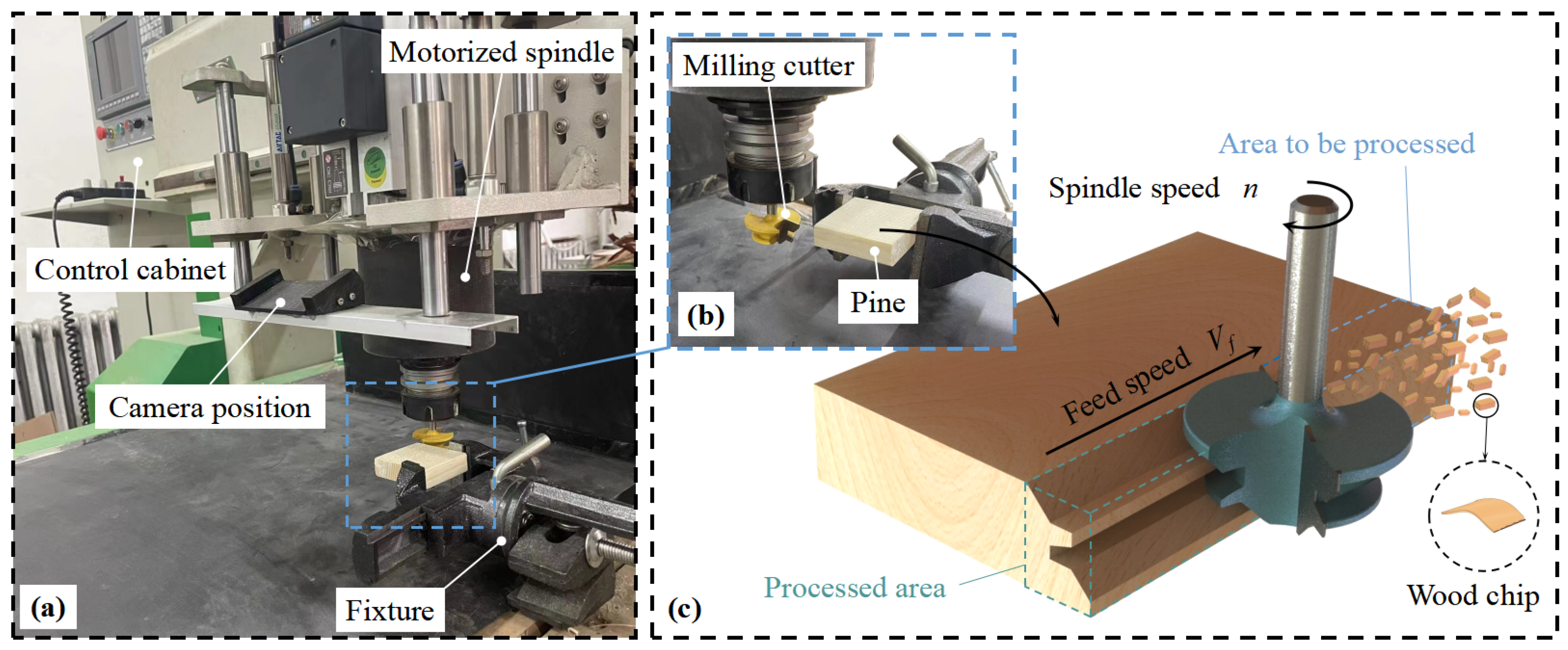
The primary focus of this study is to investigate the spreading of wood chips during circumferential milling. This particular technique of milling is frequently used in the production of tongue and groove wood, particularly in the manufacturing of doors and windows. As shown in Figure 1, the process involves circumferential milling to create the desired tongue and groove structure.
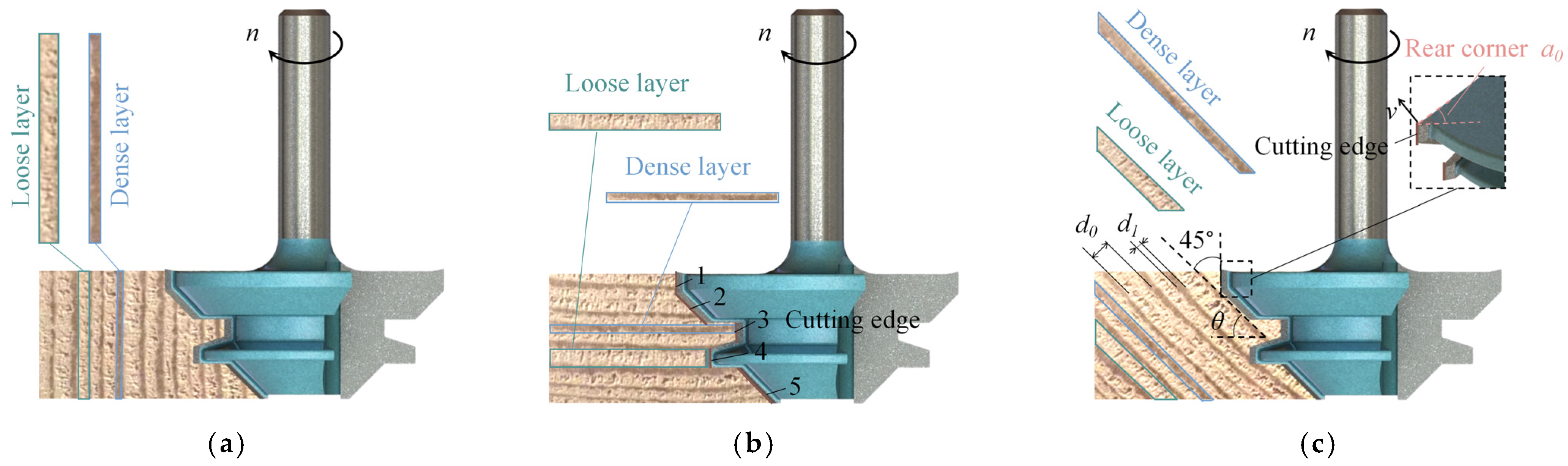
The structure of wood comprises earlywood and latewood and the boundary between them is known as annual rings. As circumferential milling is commonly used in the manufacturing of structural timber, window, and door timber, which generally have long dimensions, they are made by the radial cutting of wood. For estimation purposes, if we assume that the curvature of the annual rings is insignificant, the circumferential milling process can be roughly categorized into three groups based on the positioning of the annual rings, as depicted in Figure 2. In the figure, ɑ0 is the tool’s back angle, and the back angle of each cutting edge is equal. The front angle of each cutting edge is 0°, whereas d0 and d1 refer to the widths of the earlywood and latewood layers, respectively.
The circumferential milling cutter used in this study has a lead angle of γ0 = 0° and a back angle of ɑ0 = 30° on the cutting edge. The milling cutter is applied to the wood with the annual ring pattern shown in Figure 2a. The lengths of the cutting edges 1 to 5 are denoted by l1 to l5, and the inclination angle λ0 = 45° is applied to edges 2 and 5. Thus, the #1, #3, and #4 cutting edges are computed with single-layer properties during cutting, whereas the #2 and #5 cutting edges are calculated using multi-layer properties. For instance, if l2cosλ0 < (d0|d1) for the No. 2 cutting edge, it is computed as single-layer property, and vice versa.
Let the cutting width be aw (i.e., the width of the cutting edge), and the single cutting depth be a′c (i.e., the depth of cutting into the workpiece by the No. 1 cutting edge). The value of a′c can be expressed as a function of the feed rate Vf and spindle speed n:
The moment of inertia of the cross section to the neutral axis is as follows:
The maximum stress on the fracture surface is expressed in Equation (3), wherein MF represents the bending moment induced by the cutting chip.
Let Fc and Ft be the horizontal and vertical components of the cutting force, respectively, between the circumferential milling cutter and the wood. The equations for Fc and Ft are presented as (6) and (7) in reference [17]:
where rm is the radius of chip deflection, rf is the radius of the wood fiber sieve tube, volf is the wood fiber volume fraction, and Sm is the wood shear strength in the corresponding direction. Additionally, φ denotes the rotation angle, μ is the friction coefficient, and θ represents the angle between the annulus and the horizontal plane.
Despite having a 0° leading angle, the milling cutter’s cutting edge generates an upward force on the wood chips due to a combination of main cutting force and feed resistance. This upward force causes the chips to tear away from the wood specimen, and the magnitude of this force changes with the chips’ angle of rotation. Assuming that the angle of rotation of the wood chips at fracture is denoted by ω, the force that lifts the chips vertically upward to fracture is represented by N, the component force in the same direction as the wood fibers is denoted as Fc, and the component force perpendicular to the annual layer pointing in the direction of the wood specimen is represented by Ft. As illustrated in Figure 3, the wood chips are subjected to a force N, which can be described by the following Equation (8) [18]:
The cutting edge of the circumferential milling cutter features a leading angle γ0 of 5° and a trailing angle of ɑ0 of 30°. This cutter angle serves to enhance tool life but results in average cutting surface quality, as per previous research [17]. In Figure 3c, the wood damage mainly comprises interfiber tearing. This damage can be predicted by calculating the average bending strength σf, influenced by factors such as the percentage of earlywood and latewood layers and the gap. Equation (9) presents the prediction model for chip length L1, which is formed by the cutting edges 1, 3, and 4. Accordingly, the shape of the chip produced by these cutting edges can be approximated by a rectangular sheet of length L1, width aw, and thickness a′c, without accounting for the real-time effect of feed rate Vf on a′c.
2.2.2. Modeling of Chip Boundary Surface f(x,y)
During the pre-experiment, it was observed that the front view of the boundary shape of the wood chip diffusion region consisted of two parabolas beyond the zero point. The initial angle of the lower parabola was 0°. On the other hand, the top view of the boundary shape was symmetrical along the y-axis and consisted of two straight lines past the zero point. These observations were in line with previous studies conducted by Y.Dong [10]. The morphology of the wood chips produced by the milling process is consistent with the milling results of Wei [19]. The procedure for establishing the equations of the chip boundary surface is explained in the subsequent section.
Assuming an initial motion velocity of wood chips of V0, it must satisfy V0 = 2πnr, where r corresponds to the radius of gyration of the knife tip. Taking the air resistance coefficient as C = 0.5 and the air density as ρa = 1.3 g/L, with a maximum windward area of S = La × aw and the mass of wood chips as m, we obtain the velocity Vt of the wood chips at time t, as shown in Equation (10):
Taking the surface contained in the y+, x+, and z+ quadrants as an example, Figure 4a illustrates the expression of the y-axis and z-axis components of the displacement of M1 wood chips above the y-axis in the absence of air resistance during free fall. The M1 coordinates can be described using variables, as presented in Equation (11). The highest point reached by the wood chip can be calculated using Equation (12):
In Figure 4b, the initial velocity component of M2 in the z-direction is zero as depicted in Figure 4c. The variation laws of angles β′yoz and β′xoy for any wood chip M3 on the boundary surface are represented in Equation (13) as follows:
As one tends to its maximum value, the other always tends to zero. It is therefore assumed that the rates of change in 2β′yoz and β′xoy are linearly related. That is to say, β′yoz = kβ′xoy/2 + b. The relationship between the two angles can be solved using Equation (14) presented below:
Figure 4c illustrates projection l of the wood chip M3′s displacement in the xoy plane, as given in Equation (15). Furthermore, the time t is represented by Equation (16). Equation (18) accurately describes the relationship satisfied by β′xoy:
At this point, the coordinates of the M3 point can be described as in Equation (19):
Substitute Equation (16) into Equation (19) to eliminate time t. The result is shown in Equation (20):
Substituting Equation (14) into Equation (20), the result is shown in Equation (21):
Equation (22) provides the equation, f1(x,y), for the boundary surface of the wood chip in the x+, y+, and z+ space. The collapse of β′xoy is achieved by substituting Equation (18) into Equation (21), resulting in the following equation:
Similarly, the coordinates of the wood chip M3 in the x+, y+, and z+ space can be expressed using Equation (23). Upon completing the necessary steps, the equation for the boundary surface of the wood chip in the x+, y+, and z+ space can be obtained as shown in Equation (21), and is represented by f2(x,y):
The boundary surface of the wood chip in the x-direction is symmetric with f1(x,y) and f2(x,y) about the yoz plane. This implies that the boundary surface for the x-directional chip can be obtained by replacing x with -x. It is worth noting that in Equations (22) and (24), Vt refers to the velocity on the diffuse boundary surface at time t. By substituting Equation (16) into Equations (10), (14) and (18), we obtain the results as shown in Equation (25). The values of βyoz and βxoy are related to the spindle speed n, feed rate Vf, and depth of cut ac, which shall be regressed polynomially later.
2.3. Methods
To capture the machining process, two video recorders with a frame rate of 240 were strategically placed to record both the forward and overhead directions of the wood specimen. Subsequently, Digimizer software was utilized to measure the components of the chip spread angle in each plane.
In order to investigate the state of wood chip diffusion, a 3-factor, 5-level CCD (central composite design) test method was utilized. This particular method is capable of effectively regressing the quadratic curve while estimating the quadratic term coefficients, thereby verifying the theoretical and experimental fit [20]. Additionally, it examines the impact of test factor interactions on the test index. This method has gained widespread applications in experiments involving factors that may exceed their limits [21]. Table 2 displays the tabulated test factor levels, with the test indicators being the projected chip diffusion angle β along the x-axis βyoz, the projected angle along the z-axis βxoy, and the average chip size La. During milling operations, if the spindle speed drops below 6000 r/min, the machine will produce excessive noise and vibrations. The maximum spindle speed for the machine is 11,500 r/min; therefore, the allowable range for spindle speed n is 6000 r/min to 11,000 r/min. Similarly, the upper limit for feed speed is based on the maximum feed speed allowed by the machine of 1800 mm/min; thus, the range for feed speed Vf is 430 mm/min to 1770 mm/min. The depth of cut is also subject to the machinable range of the milling cutter, and the range for cutting depth ac is designated between 5 mm to 15 mm.
3. Results and Discussion
The test was conducted at the Forestry and Woodworking Machinery Engineering Technology Center of Northeastern Forestry University, at a temperature of 25 °C. The test consisted of 26 groups, with six of these being repeated tests to ensure that the test error remained within the allowable range. The results of the test are presented in Table 3, with the corresponding parameters shown in Figure 5. βyoz pertains to the forward-looking spreading angle, representing the projection of the chip spreading angle β along the x-axis, whereas βxoy denotes the top-looking spreading angle, representing the projection of the chip spreading angle β along the z-axis. The parameters La1 to La4 are the average chip sizes that are evenly spaced, with La representing the overall average chip size. The numbers 1 to 20 in the table correspond to the CCD test numbers, whereas 21 to 26 are the supplementary experiment numbers that were utilized to study the chip size distribution.
The test results indicated that after being separated from the wood specimen, the motion area of the chips can be broadly categorized into three types: the main diffusion area, the random diffusion area, and the vortex area, as clearly illustrated in Figure 5a. The main diffusion area denotes the primary region of motion diffusion that is observed under the influence of cutting force following chip formation. The boundary of this region remains constant over time. On the other hand, the random diffusion area pertains to the diffusion area that is formed when small parts of chips deviate from the main diffusion zone. The boundary of this region is characterized by a certain level of randomness and tends to change over time. The vortex area, on the other hand, represents the circular motion zone of chip spiral rising and settling that arises due to the turbulent surge of the circumferential milling cutter wind and the influence of gravity specifically for very fine chips (La < 0.2 mm). In this paper, we primarily focus on the main diffusion zone.
3.1. Effect of Milling Parameters on the Orthogonal Diffusion Angle βyoz
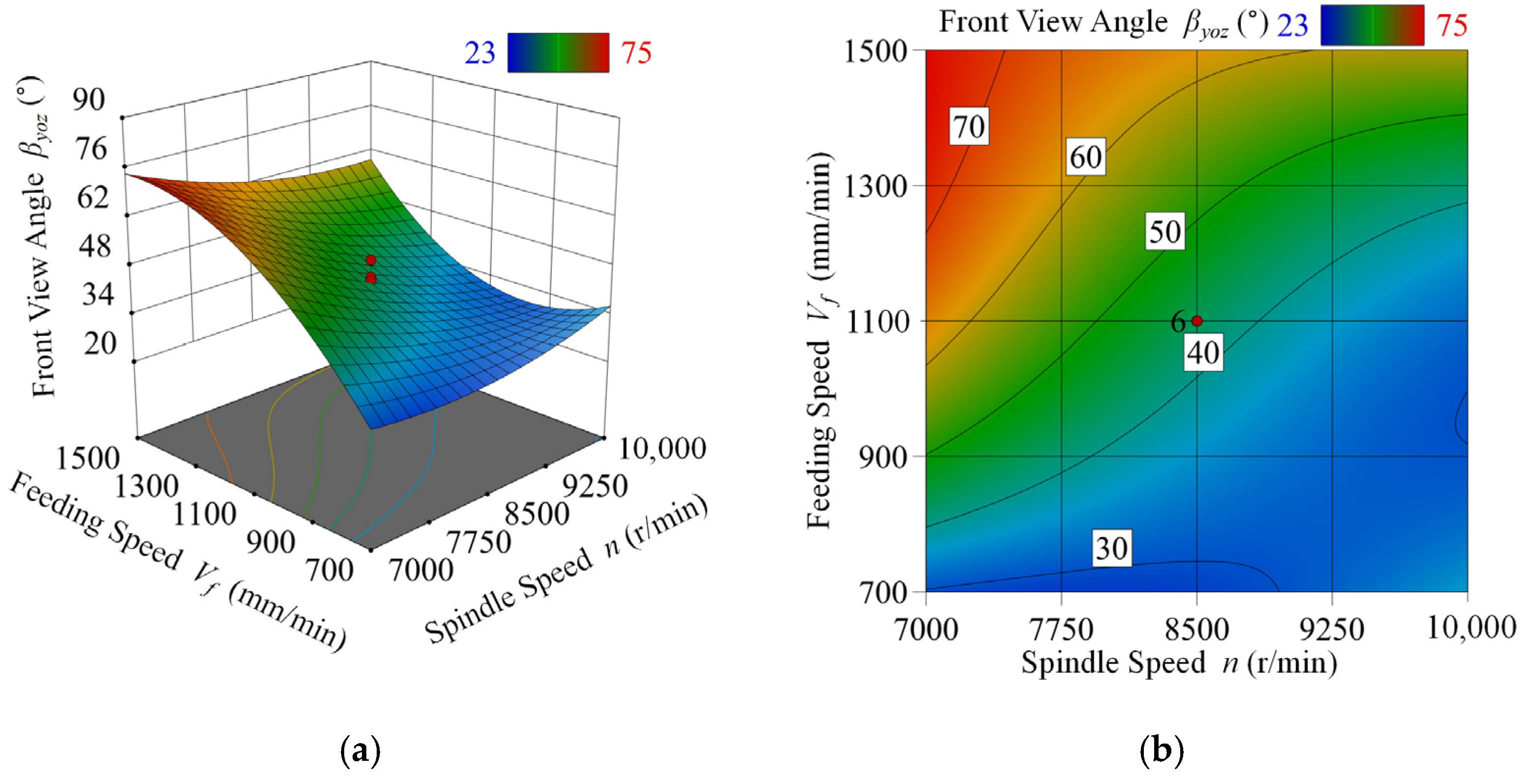
The chip motion is primarily influenced by gravity and the direction of the initial velocity, resulting in the orthogonal boundary of the main diffusion zone becoming parabolic in shape. In this regard, the orthogonal diffusion angle βyoz mentioned in this paper refers to the angle clamped by the tangent lines of the upper and lower boundaries at the initial point, as shown in Figure 5a. The analysis of the experimental data indicated that the overall model regression was highly significant (p < 0.0001). However, the depth of cut ac had almost no effect on the orthogonal diffusion angle because the p-value of ac is greater than 0.1. The analysis of variance for the regression model is presented in Table 4. The polynomial obtained from the regression has been illustrated in Equation (26). The visualization of the chip ortho-visual diffusion angle βyoz is shown in Figure 6 for better understanding.
Based on Figure 6, it can be observed that a decrease in spindle speed n or an increase in feed rate Vf results in an increase in the chip orthogonal diffusion angle βyoz. Consequently, the cutting force and its amplitude also increase [17], making the cutting condition more severe. As a result, the standard deviation of the generated chip size becomes larger and the range of the initial direction of chip movement becomes more random, leading to an increase in the area of the main diffusion zone. On the contrary, increasing spindle speed n and reducing feed speed Vf leads to a softer cutting process, with smaller chip sizes and a reduced range of initial velocity direction. This, in turn, results in a decrease in the positive diffusion angle βyoz. Notably, βyoz is found to be independent of the depth of cut ac. This suggests that the direction of the initial chip shot on the plumb plane is largely independent of the chip shape and size.
3.2. Effect of Milling Parameters on the Top View Diffusion Angle βxoy
The data analysis indicates that the regression model is significant overall (p = 0.0011). However, spindle speed n was found to have little impact on the top view diffusion angle βxoy in the experiment. Table 5 displays the analysis of variance for the regression model. To improve the regression effect, a more complex regression polynomial of βxoy was required compared to that of βyoz, as shown in Equation (27). Figure 7 depicts the visualization of the chip top view diffusion angle βxoy.
Based on the findings in Figure 7, it can be observed that the chip pitch diffusion angle βxoy generally increases with increasing depth of cut ac, and feed rate Vf. The theoretical analysis described in the previous section suggests that the chip diffusion angle in the xoy direction is determined by the direction of the chip at the moment it leaves the cutting edge. The time for this release is influenced by the centripetal force provided by the cutting force and the friction coefficient between the cutting edge and the chip. As the depth of cut and feed rate increase, the average chip size also becomes larger. This is due to the fact that large chips have a larger contact area, which causes them to break away from the cutting edge more slowly. Additionally, increasing chip size results in higher air resistance and a corresponding increase in positive pressure, ultimately slowing down the release time of the chip from the cutting edge, leading to an increase in the top view diffusion angle βxoy.
However, it was observed that pitch diffusion angle βxoy demonstrates inconsistencies with the theory in the range of ac = 7–9 mm and Vf = 900–1500 mm/min. This may be due to the fact that the depth of cut is too small for all five cutting edges of the circumferential milling cutter to be fully involved in cutting. Furthermore, at higher feed rates, chips experience greater air resistance and less collision, resulting in a deviation from the expected pattern. However, as spindle speed n increases, the chip has a greater initial velocity, which tends to eliminate the observed deviation.
3.3. Effect of Milling Parameters on the Average Chip Size La
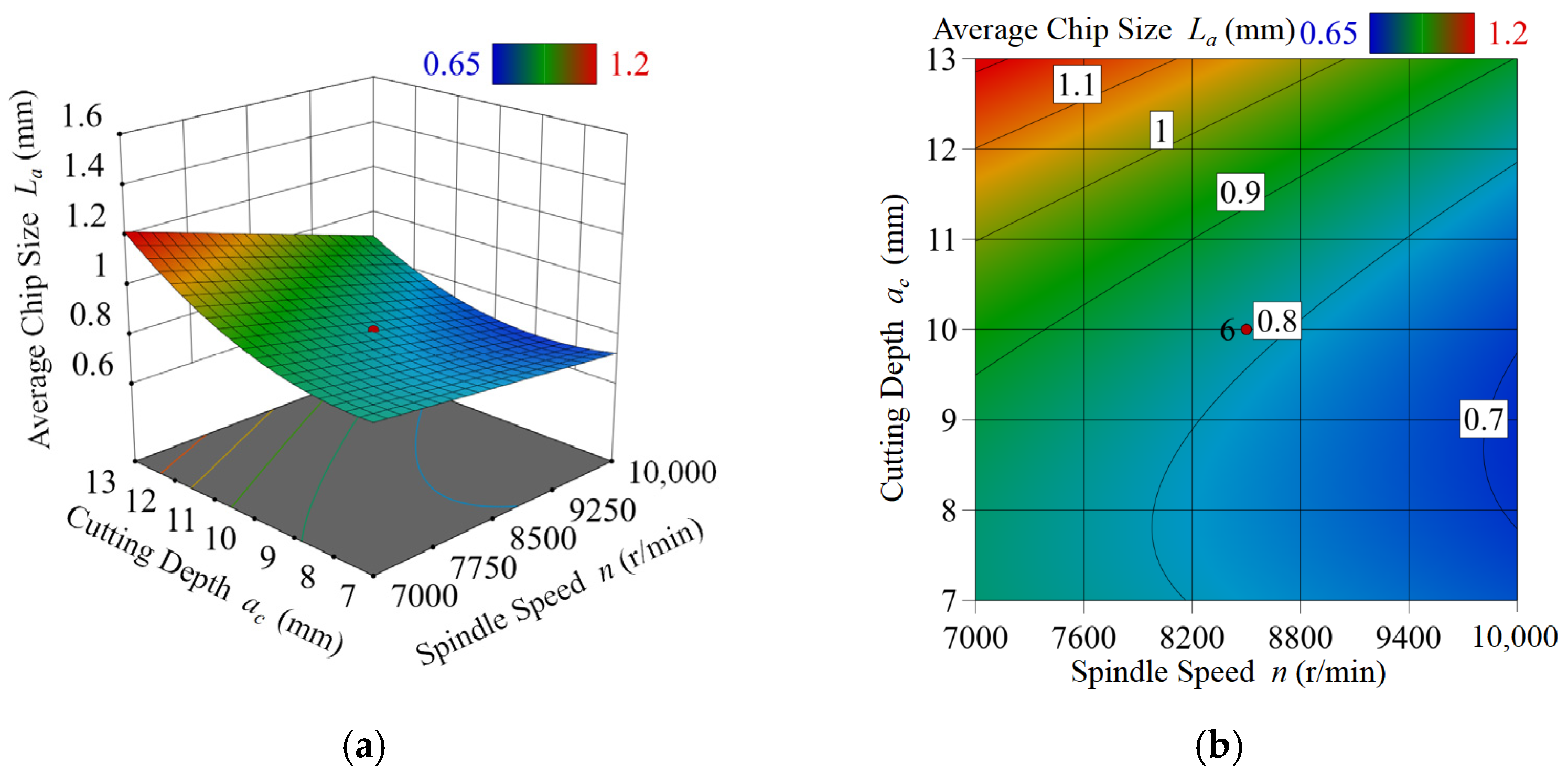
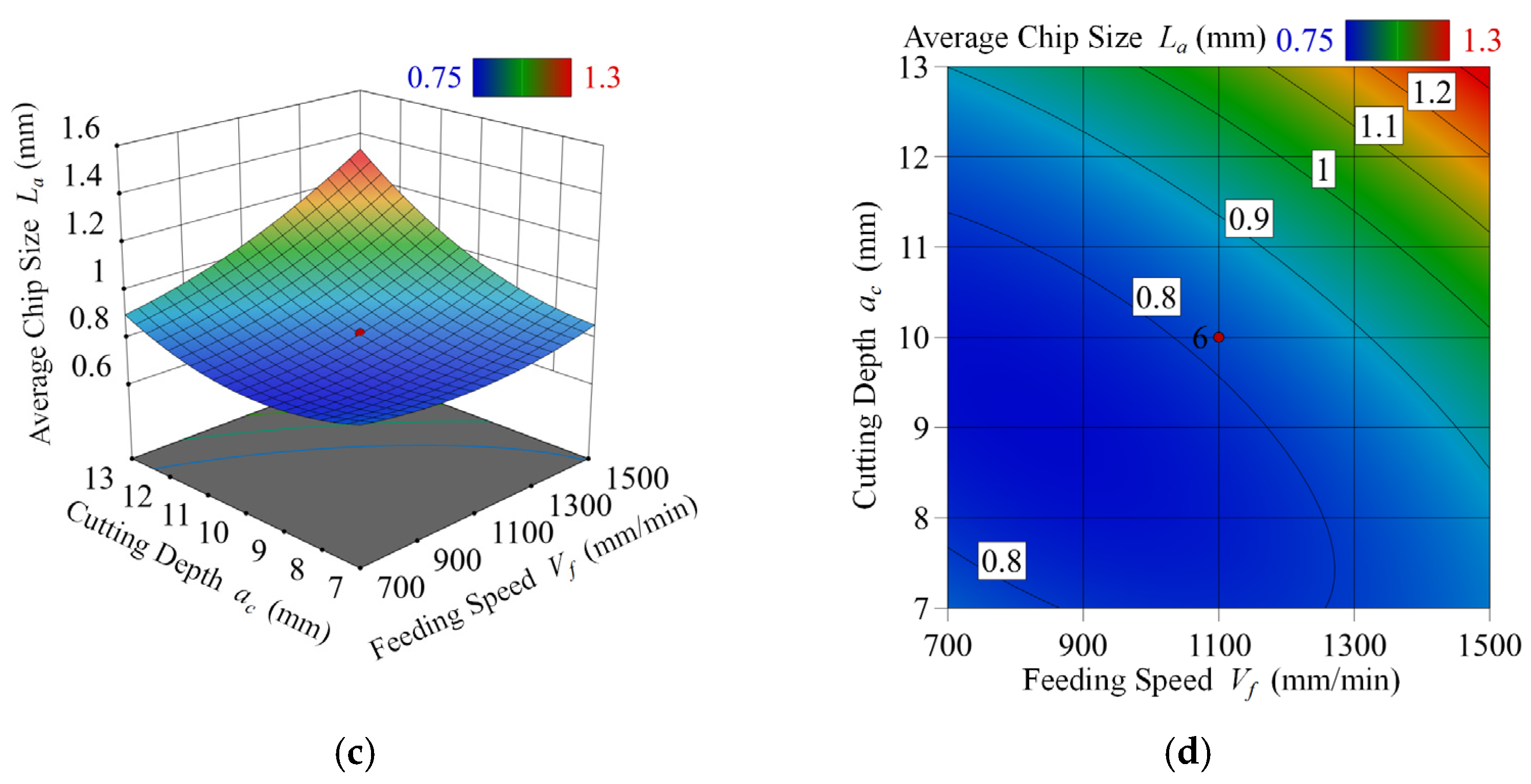
Upon analysis of the experimental data, it can be observed that the regression of the model is extremely significant with a p-value of less than 0.0001. The regression process of three individual factors, spindle speed n, feed rate Vf, and depth of cut ac, revealed that all three contributed significantly to the average chip size La (p-values less than 0.0004 for each factor). The analysis of variance for the regression model is presented in Table 6, and the regression polynomial for La can be found in Equation (28). A visualization of the mean chip size La is displayed in Figure 8.
Upon examining Figure 8, it becomes evident that the average chip size La increases as the depth of cut ac increases, the spindle speed n decreases, or the feed rate Vf increases. These results align closely with previous research in the field of wood processing [17] and are consistent with the theoretical analysis presented earlier. Notably, the depth of cut has the strongest impact on the average chip size when compared to the other variables.
3.4. Distribution State of Chip Size
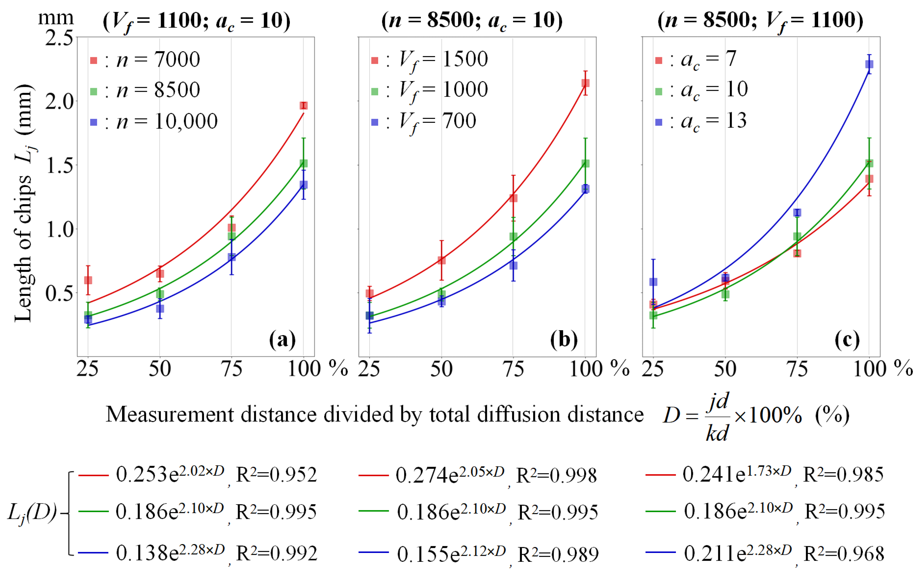
The wood specimen was milled to create a macroscopic shape of wood chips spread in a fan shape around the milling cutter. This macroscopic shape changed as the cutting parameters were varied. Four equally spaced points within the fan area were sampled, as shown in Figure 5c, and their corresponding microscopic images were captured, as demonstrated in Figure 5d. The analysis and regression of the data led to Figure 9. Despite varying the cutting parameters, the sampled relative position D consistently demonstrated a clear and significant exponential relationship with the sampled chip size Lj. The R2 value even reached 1 when performing the second-order exponential autoregression on the data. To avoid overfitting, an exponential model without constant terms was utilized in the data analysis. The regression results remained effective.
When the remaining cutting parameters remained unchanged, an increase in spindle speed n led to a more uniform distribution of the sampled chip size Lj in the sampling direction, as shown in Figure 9a. This indicates that the cutting stability increases with an increase in spindle speed n. This finding is generally consistent with the analytical results demonstrated in Figure 6 and the trend observed in the Ogun PS study [22] in terms of spindle speed and chip size. Moreover, the mean value of the sampled chip size Lj data increased as the spindle speed n increased, which is consistent with the analytical findings in Figure 8.
When the remaining cutting parameters remained unchanged, an increase in feed rate Vf led to a more uneven distribution of the sampled chip size Lj in the sampling direction, as demonstrated in Figure 9b. This indicates that the cutting stability decreases as the feed rate Vf increases, which is consistent with the analytical findings presented in Figure 6 and also in alignment with results from Ispas.M on cutting stability aspects [23]. Additionally, the mean value of the sampled chip size Lj data increased as the feed rate Vf was increased, which is in agreement with the analytical results demonstrated in Figure 8.
When the remaining cutting parameters were unchanged, an increase in the depth of cut ac led to a more uneven distribution of the sampled chip size Lj in the sampling direction. The distribution increased dramatically between ac = 10 mm and ac = 13 mm, as illustrated in Figure 9c. This indicates a decrease in cutting stability with an increase in cutting depth ac, which is consistent with the analysis results presented in Figure 7 and the findings of Ogun PS [22]. Furthermore, the mean value of the sampled chip size Lj data increased as the depth of cut ac was increased, which is consistent with the analytical findings demonstrated in Figure 8.
3.5. Solution of Chip Boundary Surface Model f(x,y)
To verify the chip boundary surface model, CCD tests No. 1, No. 11, and No. 25 were utilized. Table 7 shows the parameters used for model substitution, and the solution results obtained by substituting these parameters into Equations (1), (22), (24) and (28) are presented in Figure 10. The model considers shape errors and dimensional errors, with size errors being more appropriate to determine prediction accuracy. The actual and predicted regions are divided into 1 mm grids, and the dimensional error is described by calculating the ratio between the intersection and concatenation of the regions. It was found that the average error of the model was 32.17% after calculations.
Based on the previous theoretical analysis, it is established that the diffusion area of chips corresponds to the area enclosed by the two surfaces f1(x,y) and f2(x,y). Moreover, in situations where the distance between the milling plane and the table is 100 mm, the theoretical chip dispersal area on the table corresponds to the area enclosed by the two surfaces of f1(x,y) and f2(x,y), as well as the plane of z = −100 mm. As illustrated in Figure 10, the simulated chip boundary surfaces closely resemble the actual spread of chips generated during cutting. The area between the two surfaces effectively corresponds to the genuine chip dispersal area.
In Figure 10, some of the chips scatter outside the theoretical region. These chips can be attributed to two different factors. Firstly, a portion of them arises from the vortex zone noted in Figure 5a. Specifically, the chips located in this region are very fine and not a predominant component of the chips. Secondly, the remaining chips come from the random diffusion zone. The scattering of chips in this region is somewhat random but can produce a bias in the predicted outcomes. This issue is particularly apparent in Figure 10a, which is caused by the proximity of the chip fall. As suggested previously, the vortex zone is created by the wind force of the milling cutter. Consequently, when the chip falls closer to the milling cutter, it is more significantly influenced by the vortex zone. As such, the actual value in Figure 10a is larger than the real value. However, this error diminishes as the chip drop distance increases, as shown in Figure 10b,c.
On the one hand, it should be noted that either β′yoz or β′xoy tends towards its maximum value on one axis when the other axis approaches zero. In this study, a linear relationship was assumed between the two, as presented in Equation (14). Although this method does not affect the limited position of each axis of the wood chip diffusion boundary, the surfaces are not smoothly connected. Therefore, future research can explore the nonlinear relationship between β′yoz and β′xoy. On the other hand, as the movement process of very fine chips is difficult to observe, the vortex region caused by the wind force of the milling cutter was not analyzed in this paper. As such, future observations and studies can be carried out to investigate the movement of extremely small chips near the milling cutter. Furthermore, if we further investigate the impact of tool angle on chip diffusion boundary based on the findings of this study, it would facilitate extending the methodology proposed in this paper to a wider scope.
4. Conclusions
This study explored the diffusion state of wood chips generated during pine wood milling with different processing parameters. We established the wood chip average size model La and chip diffusion boundary surface model f(x,y) and used CCD testing to analyze the key parameters βyoz and βxoy of f(x,y), influenced by the feed rate Vf, spindle speed n, and cutting depth ac. The accuracy of the chip boundary surface f(x,y) was confirmed. The chip diffusion area was divided into the main diffusion area, random diffusion area, and vortex area based on the chip motion state. The spindle speed n and feed rate Vf had the greatest impact on the orthogonal diffusion angle of the main diffusion zone, whereas the cutting depth ac had the greatest effect on the top view diffusion angle of the main diffusion zone. Furthermore, the authors noticed that the chip size increased exponentially with the percentage of the sampling spacing, and the fitting results were highly accurate. The chip boundary surface model f(x,y) was relatively effective in predicting the morphology and diffusion state of chips generated during circumferential milling of pine wood, which is significant for chip control in the wood milling process. Lastly, this study provides guidance for future research.
Author Contributions
Conceptualization, C.Y.; methodology, T.L.; software, T.L.; validation, Y.M.; formal analysis, T.L.; investigation, T.Z.; resources, W.Q.; data curation, T.L.; writing—original draft preparation, T.L.; writing—review and editing, T.L.; visualization, C.Y.; supervision, T.L.; project administration, Y.D.; funding acquisition, W.S. All authors have read and agreed to the published version of the manuscript.
Funding
This research was funded by “Intelligent European-style wooden window double-end composite fine milling and forming maResearch on Key Technologies for Manufacturing Intelligent European-Style Wooden Window Double-End Composite Fine Milling and Forming Machine (GA21A405)” and “Fundamental Research Funds for the Central Universities (2572020DR12)”.
Institutional Review Board Statement
Not applicable.
Informed Consent Statement
Not applicable.
Data Availability Statement
Not applicable.
Acknowledgments
We thank Bo Xue and Yang Xu for the fruitful discussion on xylem anatomy and the technical aspects of the measurements.
Conflicts of Interest
The authors declare no conflict of interest.
References
- Asdrubali, F.; Ferracuti, B.; Lombardi, L.; Guattari, C.; Evangelisti, L.; Grazieschi, G. A review of structural, thermo-physical, acoustical, and environmental properties of wooden materials for building applications. Build. Environ. 2017, 114, 307–332. [Google Scholar] [CrossRef]
- Magagnotti, N.; Nannicini, C.; Sciarra, G.; Spinelli, R.; Volpi, D. Determining the Exposure of Chipper Operators to Inhalable Wood Dust. Ann. Occup. Hyg. 2013, 57, 784–792. [Google Scholar]
- Shchelokov, Y.M. Upgrading designs of cyclone dust cleaner apparatuses. Russ. J. Non-Ferr. Met. 2008, 49, 478–479. [Google Scholar] [CrossRef]
- Kamata, H.; Kanauchi, T. Analysis of roughness of cutting surface with NC router (influence of grain direction in solid wood). Trans. Jpn. Soc. Mech. Eng. Ser. C. 1994, 60, 303. [Google Scholar] [CrossRef]
- Ohuchi, T.; Murase, Y. Milling of wood and wood-based materials with a computerized numerically controlled router V: Development of adaptive control grooving system corresponding to progression of tool wear. J. Wood Sci. 2006, 2, 395–398. [Google Scholar] [CrossRef]
- Budak, E.; Alintas, Y. Modeling and control of spindles radial axes for active thermal compensation. J. Manuf. Sci. Eng. 2005, 127, 77774. [Google Scholar]
- Stan, D.A.; Nezam, S.A.; Danelsson, M.; Valente, A. Chip morphology and chip formation mechanisms in orthogonal high-speed machining of Inconel 718. Procedia CIRP 2014, 16, 61–66. [Google Scholar]
- Varga, M.; Csanady, E.; Nemeth, G.; Nemeth, S. Aerodynamic assessment of the extraction attachment of cnc processing machinery. Mater. Sci. 2006, 51, 49–62. [Google Scholar]
- Barański, J.; Jewartowski, M.; Wajs, J.; Pikala, T. Experimental analysis of chip removing system in circular sawing machine. Trieskove Beztrieskove Obrabanie Dreva. 2016, 10, 25–29. [Google Scholar]
- Dong, Y.; Bouali, A.; Mechbal, N.; Bleron, L.; Raharijaona, T. Towards wood dust collection during robotic grooving. In Proceedings of the 10th International Conference on Systems and Control (ICSC), Marseille, France, 23–25 November 2022; pp. 477–481. [Google Scholar]
- Goli, G.; Fioravanti, M.; Marchal, R.; Uzielli, L. Up-milling and down-milling wood with different grain orientations theoretical background and general appearance of the chips. Eur. J. Wood Wood Prod. 2009, 67, 257–263. [Google Scholar] [CrossRef]
- Kiliç, M.; Burdurlu, E.; Aslan, S.; Altun, S.; Tümerdem, O. The effect of surface roughness on tensile strength of the medium density fiberboard (MDF) overlaid with polyvinyl chloride (PVC). Mater. Des. 2009, 30, 4580–4583. [Google Scholar] [CrossRef]
- Darmawan, W.; Azhari, M.; Rahayu, I.S.; Nandika, D.; Dumasari, L.; Malela, I.; Nishio, S. The chips generated during up-milling and down-milling of pine wood by helical router bits. J. Indian Acad. Wood Sci. 2018, 15, 9–12. [Google Scholar] [CrossRef]
- Darmawan, W.; Tanaka, C. Discrimination of coated carbide tools wear by the features extracted from parallel force and noise level. Ann. For. Sci. 2004, 61, 731–736. [Google Scholar] [CrossRef]
- Ekevad, M.; Marklund, B.; Gren, P. Wood-chip formation in circular saw blades studied by high-speed photography. Wood Mater. Sci. Eng. 2012, 7, 115–119. [Google Scholar] [CrossRef]
- Goli, G.; Fioravanti, M.; Marchal, R.; Uzielli, L.; Busoni, S. Up-milling and down-milling wood with different grain orientations—The cutting forces behaviour. Eur. J. Wood Wood Prod. 2010, 68, 385–395. [Google Scholar] [CrossRef]
- Orlowski, K.A.; Ochrymiuk, T.; Atkins, A.; Chuchala, D. Application of fracture mechanics for energetic effects predictions while wood sawing. Wood Sci. Technol. 2013, 47, 949–963. [Google Scholar] [CrossRef]
- Calzada, K.A.; Kapoor, S.G.; DeVor, R.E.; Samuel, J.; Srivastava, A.K. Modeling and interpretation of fiber orientation-based failure mechanisms in machining of carbon fiber-reinforced polymer composites. J. Manuf. Process. 2012, 14, 141–149. [Google Scholar] [CrossRef]
- Wei, W.; Cong, R.; Xue, T.; Abraham, A.D.; Yang, C. Surface Roughness and Chip Morphology of Wood Plastic Composites Manufactured via High-speed Milling. Bioresources 2021, 16, 5733–5745. [Google Scholar] [CrossRef]
- Pengcheng, D.; Bo, C.; Jinge, G.; Kun, C.; Chengfei, Z.; Yaoyu, C.; Chenyang, X.; Yongqiu, Z. 3D Radiation Temperature Measurement of Dynamic Combustion Field Based on Multi-CCD Synchronous Coupling. Infrared Laser Eng. 2022, 51, 51–60. (In Chinese) [Google Scholar]
- Wang, Z.; Wang, G.; Xu, M.; Hao, H.; Chang, Q. Preparation of dithiocarboxyl amino-methylated polyacrylamide optimized by response surface methodology. China Environ. Sci. 2017, 37, 2114–2121. (In Chinese) [Google Scholar]
- Ogun, P.S.; Jackson, M.R.; Parkin, R.M. Mechatronic approach towards surface quality improvement in rotary wood machining. Proc. Inst. Mech. Eng. Part B J. Eng. Manuf. 2013, 1227, 1266–1276. [Google Scholar] [CrossRef]
- Ispas, M.; Gurau, L.; Campean, M.; Hacibektasoglu, M.; Racasan, S. Milling of Heat-Treated Beech Wood (Fagus sylvatica L.) and Analysis of Surface Quality. Bioresources 2017, 11, 9095–9111. [Google Scholar] [CrossRef]
- Jones, P.D.; Fox, T.R. Wood density in Pinus taeda x Pinus rigida and response 10 years after thinning in Virginia. For. Prod. J. 2007, 57, 70–73. [Google Scholar]
Figure 1.
Wood circumferential milling and wood chip diffusion state. (a) Pine specimen clamped on the machine. (b) Milling cutter fixed on the electric spindle and pine specimen fixed on the fixture. (c) Schematic diagram depicting the chip generation process.
Figure 1.
Wood circumferential milling and wood chip diffusion state. (a) Pine specimen clamped on the machine. (b) Milling cutter fixed on the electric spindle and pine specimen fixed on the fixture. (c) Schematic diagram depicting the chip generation process.

Figure 2.
Analysis of the forces during circumferential milling of wood. (a) The state when the cutting edge is parallel to the annual wheel of the wood. (b) The state when the cutting edge is perpendicular to the annual wheel of the wood. Numbers 1 to 5 refer to the serial numbers of the five cutting edges of the circumferential milling tool. (c) The state of cutting edge No. 1 when it is at an angle of 45° to the annual wheel of the wood and the parameters utilized for the calculation of the tool and the layer of the annual wheel of the wood are shown.

Figure 3.
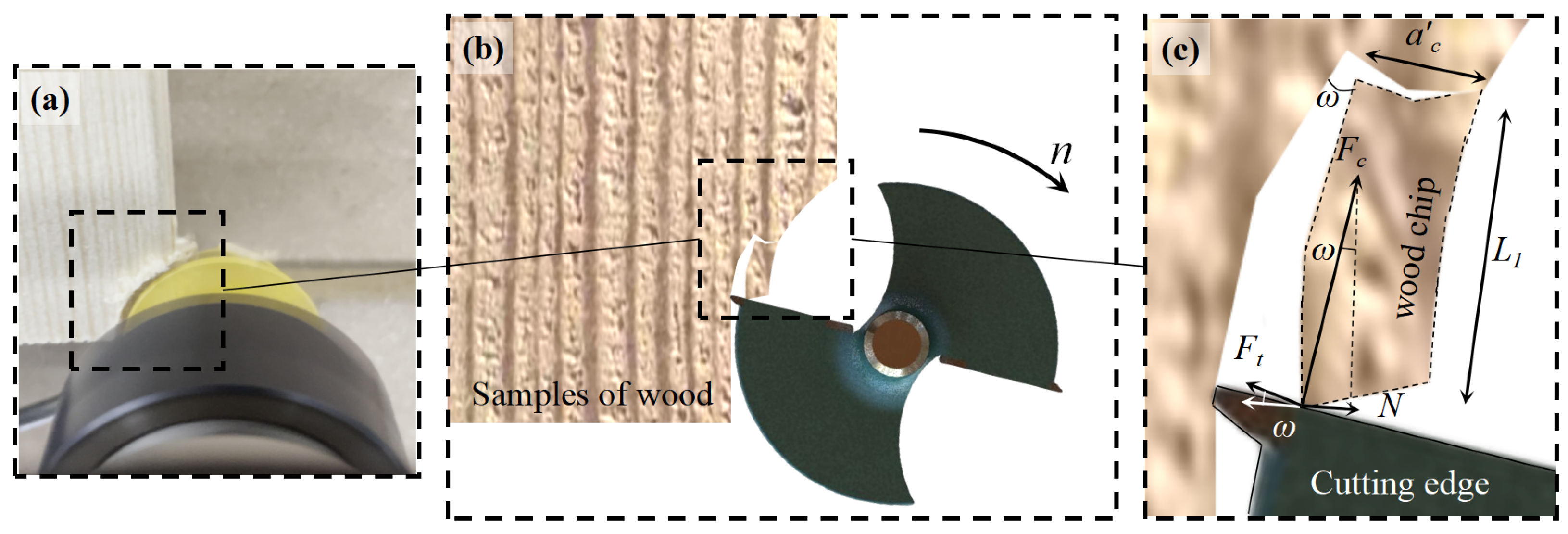
Top view of wood circumferential milling and force analysis. (a) The actual circumferential milling process of the machine. (b) A theoretical illustration of the wood circumferential milling process. (c) A local enlarged view of the wood chip formation area. The wood chip length denoted by L1 and the cutting depth represented by a′c have been amplified for labeling ease.
Figure 3.
Top view of wood circumferential milling and force analysis. (a) The actual circumferential milling process of the machine. (b) A theoretical illustration of the wood circumferential milling process. (c) A local enlarged view of the wood chip formation area. The wood chip length denoted by L1 and the cutting depth represented by a′c have been amplified for labeling ease.

Figure 4.
Boundary of the wood chip diffusion surface. (a) The boundary trajectory after the chip is detached from the milling cutter. (b) The boundary in the yoz plane. M1 is the wood chip on the boundary line of this plane. βyoz is the initial angle of the wood chip boundary in the yoz plane and the maximum angle. (c) The boundary in the xoy plane. M2 is the wood chip on the boundary line of this plane. βxoy is the initial angle of the wood chip boundary in the xoy plane and the maximum angle. (d) For any chip M3 located on the boundary surface, the angles β′yoz and β′xoy represent the inclination of the initial velocity with respect to the xoy plane and the current plane with respect to the yoz plane, respectively.

Figure 5.
Milling test results and observed chip sizes. (a) Front view of test No. 6. (b) Top view of test No. 9. (c) Test No. 6 top view of the scattered state of chip distribution after machining. Four equally spaced areas of d were taken and then photographed using a portable microscope. (d) The four white square areas in Figure (c) were photographed by a 1000× portable microscope. La1 to La4 are the average chip sizes in these four areas, respectively.

Figure 6.
Feed rate Vf and spindle speed n versus orthogonal diffusion angle βyoz at depth of cut ac = 10 mm. (a) Plot of the response surface of the orthogonal diffusion angle βyoz with respect to spindle speed n and feed rate Vf. (b) Contour plot of the response surface.
Figure 6.
Feed rate Vf and spindle speed n versus orthogonal diffusion angle βyoz at depth of cut ac = 10 mm. (a) Plot of the response surface of the orthogonal diffusion angle βyoz with respect to spindle speed n and feed rate Vf. (b) Contour plot of the response surface.

Figure 7.
Depth of cut ac and feed rate Vf at spindle speed n = 8500 r/min versus the pitch diffusion angle βxoy. (a) Plot of the response surface of the overhead diffusion angle βxoy with respect to the depth of cut ac and feed rate Vf. (b) Contour plot of the response surface.
Figure 7.
Depth of cut ac and feed rate Vf at spindle speed n = 8500 r/min versus the pitch diffusion angle βxoy. (a) Plot of the response surface of the overhead diffusion angle βxoy with respect to the depth of cut ac and feed rate Vf. (b) Contour plot of the response surface.

Figure 8.
Relationship between the average chip size La and feed rate Vf, spindle speed n, and depth of cut ac. (a) Response surface plot of average chip size La as a function of depth of cut ac and spindle speed n. (b) Contour plot of the response surface (a). (c) Response surface plot of average chip size La as a function of depth of cut ac and feed rate Vf. (d) Contour plot of the response surface (c).


Figure 9.
The relationship between sampling relative position D and the sampled chip size Lj at different cutting parameters is depicted as Lj(D), where d represents the sample spacing, j denotes the current sampling sequence, and k represents the total number of samples. The sampling relative position is expressed by (j/k)d × 100% within the range of 0% to 100%. (a) The change in Lj(D) after changing the spindle speed n when the feed speed Vf = 1100 and the depth of cut ac = 10. (b) The change in Lj(D) after changing the feed rate Vf when the spindle speed n = 8500 and the depth of cut ac = 10. (c) The change in Lj(D) after changing the depth of cut ac at spindle speed n = 8500 and feed rate Vf = 1100.

Figure 10.
The results of solving the f(x,y) model with different milling parameters. (a) The surface model f(x,y) was implemented and the actual chip scattering area was calculated using data from test No. 1. The error of area is 39.59%. (b) The surface model f(x,y) was implemented and the actual chip scattering area was calculated using data from test No. 11. The error of area is 27.71%. (c) The surface model f(x,y) was implemented and the actual chip scattering area was calculated using data from test No. 25. The error of area is 35.08%.


Table 1.
Mechanical properties of smooth grain pine wood.
| Density (kg/m3) | Compressive Strength (MPa) | Bending Strength (MPa) | Tensile Strength (MPa) | Shear Strength (MPa) | Modulus of Elasticity (MPa) | Poisson’s Ratio | Coefficient of Friction |
|---|---|---|---|---|---|---|---|
| 420 | 50 | 87 | 104 | 10 | 12,000 | 0.65 | 0.35 |
Table 2.
Factors and levels of the CCD test.
| Alpha | Spindle Speed n (r/min) | Feeding Speed Vf (mm/min) | Cutting Depth ac (mm) |
|---|---|---|---|
| +1.68 | 11,000 | 1770 | 15 |
| +1 | 10,000 | 1500 | 13 |
| 0 | 8500 | 1100 | 10 |
| −1 | 7000 | 700 | 7 |
| −1.68 | 6000 | 430 | 5 |
Table 3.
CCD test results and supplementary test results.
| No. | Factors | Indicators | ||||||||
|---|---|---|---|---|---|---|---|---|---|---|
| n | Vf | ac | βyoz | βxoy | La1 | La2 | La3 | La4 | La | |
| (r/min) | (mm/min) | (mm) | (°) | (°) | (mm) | (mm) | (mm) | (mm) | (mm) | |
| 1 | 7000 | 700 | 7 | 25 | 134 | 0.382 | 0.692 | 1.031 | 1.812 | 0.9792 |
| 2 | 10,000 | 700 | 13 | 31 | 107 | 0.484 | 0.541 | 0.771 | 1.396 | 0.7980 |
| 3 | 10,000 | 1500 | 13 | 73 | 135 | 0.322 | 0.559 | 1.82 | 1.9975 | 1.1746 |
| 4 * | 8500 | 1100 | 10 | 44 | 120 | 0.258 | 0.462 | 1.048 | 1.51 | 0.8195 |
| 5 | 8500 | 430 | 10 | 26 | 115 | 0.237 | 0.457 | 0.855 | 1.251 | 0.7000 |
| 6 | 11,000 | 1100 | 10 | 32 | 114 | 0.356 | 0.549 | 0.788 | 1.455 | 0.7870 |
| 7 * | 8500 | 1100 | 10 | 40 | 113 | 0.354 | 0.513 | 0.823 | 1.404 | 0.7735 |
| 8 | 7000 | 1500 | 13 | 73 | 140 | 0.514 | 1.139 | 1.793 | 2.538 | 1.4960 |
| 9 | 7000 | 700 | 13 | 28 | 114 | 0.381 | 0.563 | 1.168 | 2.47 | 1.1455 |
| 10 * | 8500 | 1100 | 10 | 43 | 115 | 0.295 | 0.488 | 0.941 | 1.455 | 0.7948 |
| 11 | 10,000 | 700 | 7 | 36 | 141 | 0.296 | 0.593 | 0.855 | 1.105 | 0.7123 |
| 12 | 8500 | 1770 | 10 | 78 | 152 | 0.542 | 0.771 | 1.357 | 2.354 | 1.2560 |
| 13 | 7000 | 1500 | 7 | 74 | 94 | 0.319 | 0.469 | 0.775 | 1.63 | 0.7983 |
| 14 | 8500 | 1100 | 15. | 45 | 137 | 0.395 | 0.668 | 0.888 | 3.11 | 1.2653 |
| 15 | 8500 | 1100 | 5 | 41 | 93 | 0.341 | 0.635 | 0.918 | 1.903 | 0.9493 |
| 16 * | 8500 | 1100 | 10 | 44 | 119 | 0.324 | 0.474 | 0.914 | 1.427 | 0.7848 |
| 17 * | 8500 | 1100 | 10 | 45 | 110 | 0.289 | 0.497 | 0.911 | 1.455 | 0.7880 |
| 18 | 10,000 | 1500 | 7 | 44 | 117 | 0.362 | 0.714 | 0.727 | 1.378 | 0.7953 |
| 19 * | 8500 | 1100 | 10 | 50 | 113 | 0.233 | 0.485 | 0.944 | 1.457 | 0.7798 |
| 20 | 6000 | 1100 | 10 | 86 | 105 | 0.291 | 0.567 | 1.4853 | 1.919 | 1.0656 |
| 21 | 10,000 | 1100 | 10 | 33 | 115 | 0.291 | 0.375 | 0.779 | 1.345 | 0.6975 |
| 22 | 7000 | 1100 | 10 | 44 | 110 | 0.597 | 0.648 | 1.008 | 1.964 | 1.0543 |
| 23 | 8500 | 1500 | 10 | 65 | 143 | 0.496 | 0.755 | 1.241 | 2.14 | 1.1580 |
| 24 | 8500 | 700 | 10 | 36 | 131 | 0.325 | 0.434 | 0.715 | 1.314 | 0.6970 |
| 25 | 8500 | 1100 | 13 | 48 | 142 | 0.585 | 0.618 | 1.127 | 2.285 | 1.1538 |
| 26 | 8500 | 1100 | 7 | 63 | 105 | 0.409 | 0.594 | 0.809 | 1.391 | 0.8008 |
* The number of the repeated test.
Table 4.
The ANOVA results for the orthogonal diffusion angle βyoz are as follows: R2 = 0.9105; adjusted R2 = 0.8692; predicted R2 = 0.7014; adeq precision = 15.6975. Notably, the overall model regression is highly significant, with a probability of noise affecting the model being only 0.01 as indicated by the F-value of 22.04. Although almost all items in the table are highly significant (p < 0.05), item B2 is not significant (p > 0.1).
| Source | Sum of Squares | df | Mean Square | F-Value | p-Value |
|---|---|---|---|---|---|
| Model | 5990.94 | 6 | 998.49 | 22.04 | <0.0001 |
| A–n | 1458 | 1 | 1458 | 32.19 | <0.0001 |
| B–Vf | 3922.62 | 1 | 3922.62 | 86.6 | <0.0001 |
| AB | 242 | 1 | 242 | 5.34 | 0.0378 |
| A2 | 297.09 | 1 | 297.09 | 6.56 | 0.0237 |
| B2 | 60.76 | 1 | 60.76 | 1.34 | 0.2676 |
| AB2 | 654.53 | 1 | 654.53 | 14.45 | 0.0022 |
| Residual | 588.86 | 13 | 45.3 | - | - |
| Lack of Fit | 535.53 | 8 | 66.94 | 6.28 | 0.0592 |
| Pure Error | 53.33 | 5 | 10.67 | - | - |
| Cor Total | 6579.8 | 19 | - | - | - |
Table 5.
The ANOVA results for the topographic diffusion angle βxoy are as follows: R2 = 0.8563; adjusted R2 = 0.7518; predicted R2 = 0.5842; adeq precision = 9.5991. Notably, the overall regression of the model is significant at p = 0.0011. The F-value of 8.19 indicates that the model is primarily influenced by signal rather than noise, with only a probability of 0.11 of being affected by noise. Furthermore, all items in the table are significant except for A and A2, with p < 0.05 indicating high significance, 0.1 < p < 0.05 indicating significance, and p > 0.1 signifying insignificance.
| Source | Sum of Squares | df | Mean Square | F-Value | p-Value |
|---|---|---|---|---|---|
| Model | 4021.77 | 8 | 502.72 | 8.19 | 0.0011 |
| A–n | 80.4 | 1 | 80.4 | 1.31 | 0.2767 |
| B–Vf | 199.72 | 1 | 199.72 | 3.25 | 0.0986 |
| C–ac | 968 | 1 | 968 | 15.77 | 0.0022 |
| AC | 220.5 | 1 | 220.5 | 3.59 | 0.0846 |
| BC | 1740.5 | 1 | 1740.5 | 28.36 | 0.0002 |
| A2 | 26.33 | 1 | 26.33 | 0.4291 | 0.5259 |
| B2 | 742.04 | 1 | 742.04 | 12.09 | 0.0052 |
| A2C | 463.85 | 1 | 463.85 | 7.56 | 0.0189 |
| Residual | 675.03 | 11 | 61.37 | - | - |
| Lack of Fit | 601.03 | 6 | 100.17 | 6.77 | 0.0566 |
| Pure Error | 74 | 5 | 14.8 | - | - |
| Cor Total | 4696.8 | 19 | - | - | - |
Table 6.
The model’s R2 value, adjusted R2 value, and predicted R2 value were determined to be 0.9201, 0.8735, and 0.6484, respectively, with an adeq precision value of 16.9314. The overall regression of the model is considered to be highly significant, with a p-value less than 0.0001. The F-value of 19.74 indicates that the probability of the model being influenced solely by noise is only 0.01. All variables included in the table are significant, with p < 0.05 indicating high significance, 0.1 < p < 0.05 indicating significance, and p > 0.1 signifying insignificance.
| Source | Sum of Squares | df | Mean Square | F-Value | p-Value |
|---|---|---|---|---|---|
| Model | 0.903 | 7 | 0.129 | 19.74 | <0.0001 |
| A–n | 0.1679 | 1 | 0.1679 | 25.69 | 0.0003 |
| B–Vf | 0.1792 | 1 | 0.1792 | 27.42 | 0.0002 |
| C–ac | 0.2535 | 1 | 0.2535 | 38.79 | <0.0001 |
| AC | 0.0199 | 1 | 0.0199 | 3.04 | 0.0994 |
| BC | 0.0851 | 1 | 0.0851 | 13.02 | 0.0036 |
| B2 | 0.0514 | 1 | 0.0514 | 7.87 | 0.0159 |
| C2 | 0.1608 | 1 | 0.1608 | 24.61 | 0.0003 |
| Residual | 0.0784 | 12 | 0.0065 | - | - |
| Lack of Fit | 0.0771 | 7 | 0.011 | 42.32 | 0.06 |
| Pure Error | 0.0013 | 5 | 0.0003 | - | - |
| Cor Total | 0.9814 | 19 | - | - | - |
Table 7.
Parameters necessary for solving the model are listed in the table below. Specifically, dc represents the chip thickness and is also equivalent to the single depth of cut a′c, which is calculated using Equation (1). Additionally, ρwood denotes the density of pine wood [24].
Table 7.
Parameters necessary for solving the model are listed in the table below. Specifically, dc represents the chip thickness and is also equivalent to the single depth of cut a′c, which is calculated using Equation (1). Additionally, ρwood denotes the density of pine wood [24].
| No. | βyoz | βxoy | g | n | Vf | r | La | aw | dc | ρwood |
|---|---|---|---|---|---|---|---|---|---|---|
| (°) | (°) | (N/s2) | (r/min) | (mm/s) | (mm) | (mm) | (mm) | (mm) | (kg/m3) | |
| 1 | 25 | 134 | 9.8 | 7000 | 11.67 | 15 | 0.979 | 0.489 | 8.34 × 10⁻⁴ | 450 |
| 11 | 36 | 141 | 9.8 | 10,000 | 11.67 | 15 | 0.712 | 0.356 | 3.50 × 10⁻⁵ | 450 |
| 25 | 48 | 142 | 9.8 | 8500 | 18.33 | 15 | 1.154 | 2.308 | 6.47 × 10⁻⁵ | 450 |
Disclaimer/Publisher’s Note: The statements, opinions and data contained in all publications are solely those of the individual author(s) and contributor(s) and not of MDPI and/or the editor(s). MDPI and/or the editor(s) disclaim responsibility for any injury to people or property resulting from any ideas, methods, instructions or products referred to in the content. |
© 2023 by the authors. Licensee MDPI, Basel, Switzerland. This article is an open access article distributed under the terms and conditions of the Creative Commons Attribution (CC BY) license (https://creativecommons.org/licenses/by/4.0/).
Share and Cite
MDPI and ACS Style
Yang, C.; Liu, T.; Ma, Y.; Qu, W.; Ding, Y.; Zhang, T.; Song, W. Study of the Movement of Chips during Pine Wood Milling. Forests 2023, 14, 849. https://doi.org/10.3390/f14040849
AMA Style
Yang C, Liu T, Ma Y, Qu W, Ding Y, Zhang T, Song W. Study of the Movement of Chips during Pine Wood Milling. Forests. 2023; 14(4):849. https://doi.org/10.3390/f14040849
Chicago/Turabian StyleYang, Chunmei, Tongbin Liu, Yaqiang Ma, Wen Qu, Yucheng Ding, Tao Zhang, and Wenlong Song. 2023. "Study of the Movement of Chips during Pine Wood Milling" Forests 14, no. 4: 849. https://doi.org/10.3390/f14040849
Note that from the first issue of 2016, this journal uses article numbers instead of page numbers. See further details here.