Coupling of SWAT and EPIC Models to Investigate the Mutual Feedback Relationship between Vegetation and Soil Erosion, a Case Study in the Huangfuchuan Watershed, China

Abstract

Identifying the feedback relationship between soil erosion and vegetation growth would contribute to sustainable watershed management. In order to study the long-term interaction between soil erosion and vegetation change, a comprehensive modeling framework was proposed by combining the Soil and Water Assessment Tool (SWAT) and the Environmental Policy Integrated Climate (EPIC) model. The Huangfuchuan Watershed was taken as an example area due to serious erosion and large-scale conversion of farmland to forest. Based on long-term variation analyses from 1956 to 2020, the effect of land cover change on runoff and sediment discharge was quantified using SWAT to create scenario simulations, and then environmental stresses factors (i.e., soil water content, nitrogen, and phosphorus contents) output by SWAT were input into EPIC to evaluate effects of soil erosion on potential biomass of vegetation. Results showed that the annual runoff reduction was 32.5 million m3 and the annual sediment reduction was 15 million t during the past 65 years. The scenario we created using the SWAT simulation showed that both forest and grassland reduced water yield, while bare land increased water yield by 10%. In addition, grassland and forest reduced soil erosion by 20% and 18%, respectively, while bare land increased sand production by 210%. The EPIC model results exhibited a negative correlation between the potential for vegetation biomass and erosion intensity. The average annual potential biomass of forest and grass under micro-erosion was 585.7 kg/ha and 485.9 kg/ha, respectively, and was 297.9 kg/ha and 154.6 kg/ha, respectively, under the extremely strong erosion. The results of this study add to the body of information regarding how soil erosion and vegetation biomass interact with each other. The proposed coupled SWAT-EPIC strategy may provide a way for further investigating the quantitative relationship between soil erosion and vegetation cover.

1. Introduction

Soil erosion is an ecological stress that affects the growth of vegetation. Soil erosion is also counteracted by vegetation; in fact, surface vegetation is important in reducing soil erosion [1,2]. Additionally, vegetation is an essential component of the material cycle and energy exchange in an ecosystem, and the presence of vegetation is the material basis for preventing ecological degradation. The growth and development of vegetation limits soil erosion through various external and internal factors. However, soil erosion, as the main driving force of ecosystem degradation, also seriously affects and interferes with vegetation growth and development. In an environment with severe soil erosion, vegetation growth is severely constrained. In summary, soil erosion and vegetation growth are interrelated and mutually exclusive, thus understanding their feedback relationship is of great significance for sustainable watershed management.

On one hand, vegetation coverage can reduce soil erosion by redistributing rainfall, preventing soil erosion from rainfall splash, improving soil structure, and reducing surface rainfall production flow [3,4]. Nowadays, there are three commonly used approaches to quantitatively describe the contribution of different vegetation cover characteristics to soil erosion: the paired watershed method [5], the statistical analysis method [6], and the modeling method [7]. Hydrological and soil erosion models are important tools for evaluating the effects of vegetation coverage on water and sediment discharges at a watershed scale. Models can be used to evaluate soil moisture, nutrient changes, and degree of soil erosion; to estimate the spatial distribution of soil erosion; and to quantify the contribution of key influencing factors [8]. The Soil and Water Assessment Tool (SWAT) model is widely used to evaluate the impacts of climate, vegetation cover, and human activities on water and sediment processes. Wang et al. [9] successfully constructed the SWAT model for the Loess Plateau, and the simulation results showed that the change of surface runoff had an impact on forest restoration, soil flow, and basic water flow. Gao et al. [10] used SWAT to build a runoff simulation for the Loess Plateau and calculated the influence of climate and human factors on runoff variability by comparing simulation results based on different modeling scenarios. Shi et al. [11] used the data simulated by the modified SWAT model to analyze the temporal variation of soil loss and total nitrogen and phosphorus loss over months and years as well as the spatial variation at the sub-basin scale in the Loess Plateau. Huo et al. [12] used SWAT to simulate five scenarios of a typical watershed Yanwachuan gully in the Loess Plateau, and they analyzed the response of runoff, sediment, and evapotranspiration under different scenarios of the Gully Consolidation and Highland Protection (GCHP) project.

On the other hand, however, research on the effects of soil erosion on vegetation growth is comparatively limited. Soil erosion is associated with a range of soil environmental factors (including soil particles, organic matter, nutrients, water, etc.), and its effects on vegetation are all-encompassing. Soil erosion can cause loss of soil particles and nutrients, and reduce the water holding capacity of the soil, which in turn can induce stress in plants. Surface runoff and sediment transport can also carry away seeds scattered on the slope, deteriorating the growth environment of vegetation and affecting the community structure and spatial distribution of vegetation. Vegetation transpiration and biomass accumulation are influenced by soil moisture and nutrient content, a finding that further shows how vegetation and the presence of soil are interdependent components in ecosystems [13]. Currently, most studies use field survey methods [14,15], the remote sensing interpretation method [16,17], and the model estimation method [18,19] to investigate the growth of vegetation under different erosion conditions. Among them, the Environmental Policy Integrated Climate (EPIC) model performs well in simulating vegetation growth. The EPIC model is nested with the hydrological cycle module, the climate module, and the soil erosion module. Therefore, it is good at simulating water use efficiency and vegetation growth. Iiames et al. [20] used the EPIC model to simulate the comparison of leaf area index at multiple spatial scales. Guo et al. [21] used the EPIC model to explore soil changes caused by the return of crops to forest and grass on the Loess Plateau.

Because of the complex interaction mechanism between soil erosion and vegetation growth, in this study, a comprehensive modeling framework and new research direction were proposed by combining the SWAT model and the EPIC model and by adopting an “output-input” [22] approach. First, we simulated the land surface hydrological cycle using the SWAT model. Specifically, we used this model to explore the temporal and spatial variations of water and sediment yield under different vegetation cover scenarios for a certain watershed and under vegetation growth stress factors, i.e., soil water content and nutrient content. Then, the obtained environmental stress factors were used as input conditions in the EPIC model to simulate the vegetation growth process, and the potential biomass was used to compare the growth of woodland and grassland under different erosion intensities. The severe soil erosion and the fragile vegetation growth environment of the Loess Plateau make it a suitable site for estimating the feedback interaction between soil erosion and vegetation growth [23].

The aims of this study were as follows: (1) to determine the long-term variations in vegetation, runoff, and sediment discharge within the Huangfuchuan Watershed of the Loess Plateau, China; (2) to quantify the effects of vegetation growth on soil erosion and the effects of soil erosion on vegetation growth; and (3) to explore an approach to investigate the feedback effects of vegetation and soil erosion by means of coupled modeling. The results of this study are expected to provide a better understanding of the feedback relationship between soil erosion and vegetation growth, which could provide more and new insights for developing an effective ecological restoration of the Loess Plateau.

2. Materials and Methods

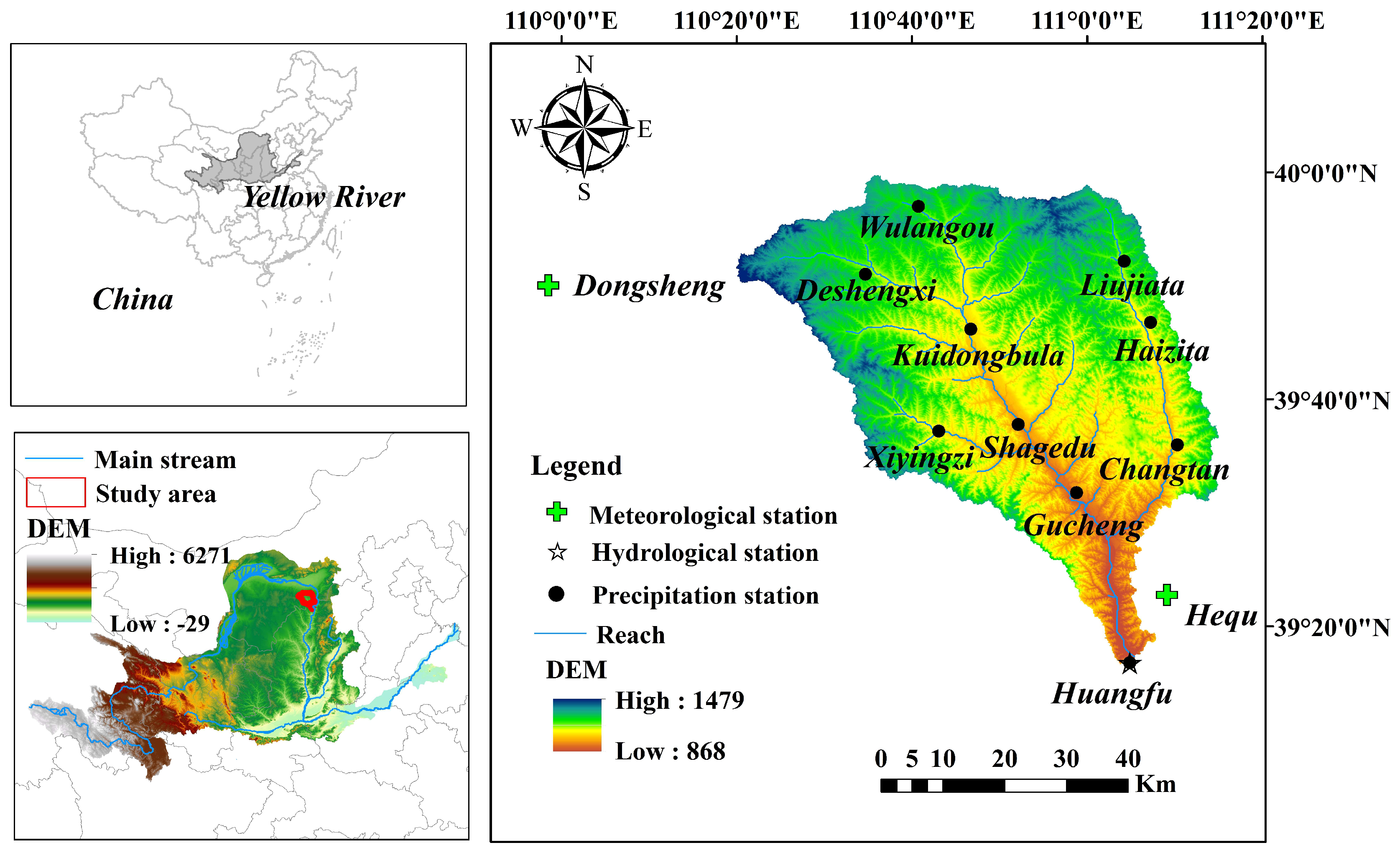
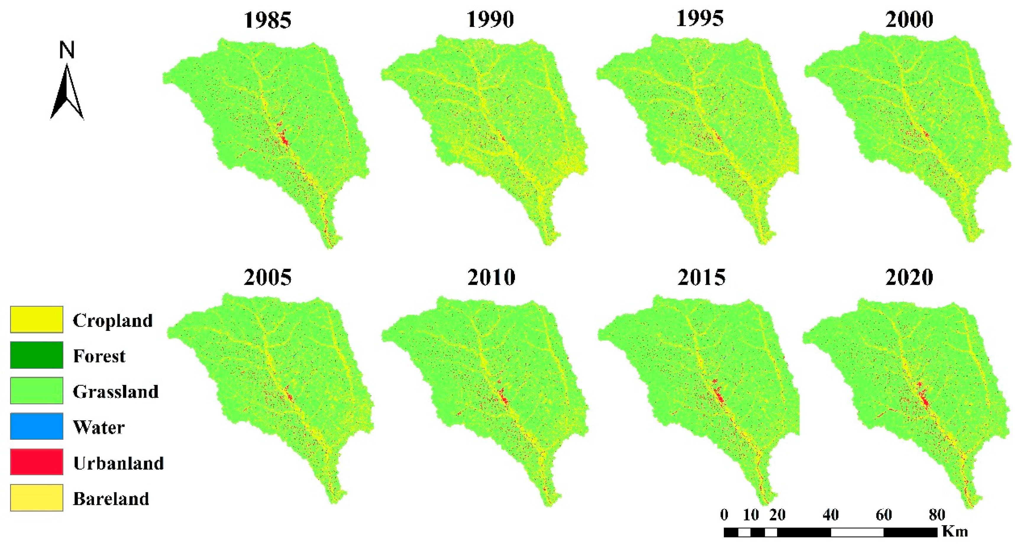
2.1. Study Area and Data

The Huangfuchuan Watershed (110.3°~111.2° E, 39.2°~39.9° N) is located on the Loess Plateau, China, and is one of the most eroded areas worldwide. Huangfuchuan is the first tributary of the Yellow River, composed of Shilichangchuan, Nalinchuan, and other major tributaries. The main river is 137 km long and the watershed area is 3246 km² (Figure 1). The Huangfuchuan Watershed belongs to a continental monsoon climate with an annual average temperature of 9.1 °C, and an annual average precipitation of 350–450 mm. Precipitation is mainly concentrated in summer, usually in the form of heavy storms, accounting for more than 80% of the annual total [24], and its distribution shows a decreasing trend from southeast to northwest. Multiple floods in summer and extreme precipitation events lead to severe soil erosion and high sediment yield [25,26,27].

The Huangfuchuan Watershed belongs to the typical steppe vegetation zone with few natural forests. The land-use types of the watershed are mainly grassland, cultivated land, and forest, with grassland accounting for more than 65% of the basin area. The soil types mainly include chestnut soil and coarse-grained sandstone (Pisha stone), which is one of the main sources of coarse sediment in the Yellow River. Annual average sediment inflow to the Yellow River is about 0.41 million tons, and the annual sediment transport modulus in the watershed is 12,733 t/(km²·a) [28].

The data required for this study consisted of spatial and attribute datasets. Basic spatial datasets included the MODIS-NDVI datasets from NASA (http://ladsweb.nascom.nasa.gov (accessed on 10 March 2022 )), the Digital Elevation Model from the Geospatial Data Cloud (http://www.gscloud.cn/ (accessed on 25 December 2021)), land-use maps from the Resource and Environment Science and Data Center (https://www.resdc.cn/ (accessed on 5 March 2022)), and soil type data from the Harmonized World Soil Database (HWSD) v1.2 [29]. The spatial resolution of MODIS-NDVI datasets was 250 m, and the spatial resolution of the other datasets was 30 m. Attribute datasets included meteorological data and hydrological data. Attribute datasets included meteorological data and hydrological data. Daily meteorological data from 1960 to 2020 were obtained from the Data and Information Center of the China Meteorological Administration (http://cdc.cma.gov.cn/home.do (accessed on 12 August 2021)) and included precipitation, temperature, wind speed, relative humidity, and solar radiation. Hydrological data were obtained from the Yellow River Conservancy Commission of the Ministry of Water Resources (http://www.yrcc.gov.cn/ (accessed on 24 July 2021)). Note that the runoff and sediment discharge records we used are from the Huangfu hydrologic station at the outlet of the watershed, and the precipitation series were provided by 12 rainfall stations as shown in Figure 1. Time series data were processed by Origin 2018 software to generate images, and spatial data were processed by Arcgis 10.2 software to generate images.

2.2. Statistical Analysis

2.2.1. Linear Fitting Method

Linear fitting method is a simple method of determining the trend of change, using regression analysis to determine the relationship between variables and statistical method, using a straight line to represent the relationship between elements (x) and elements (y), to establish a one-dimensional linear regression equation; the calculation formula is:

$$y=ax+b$$

(1)

where a and b are the regression slope and intercept, respectively.

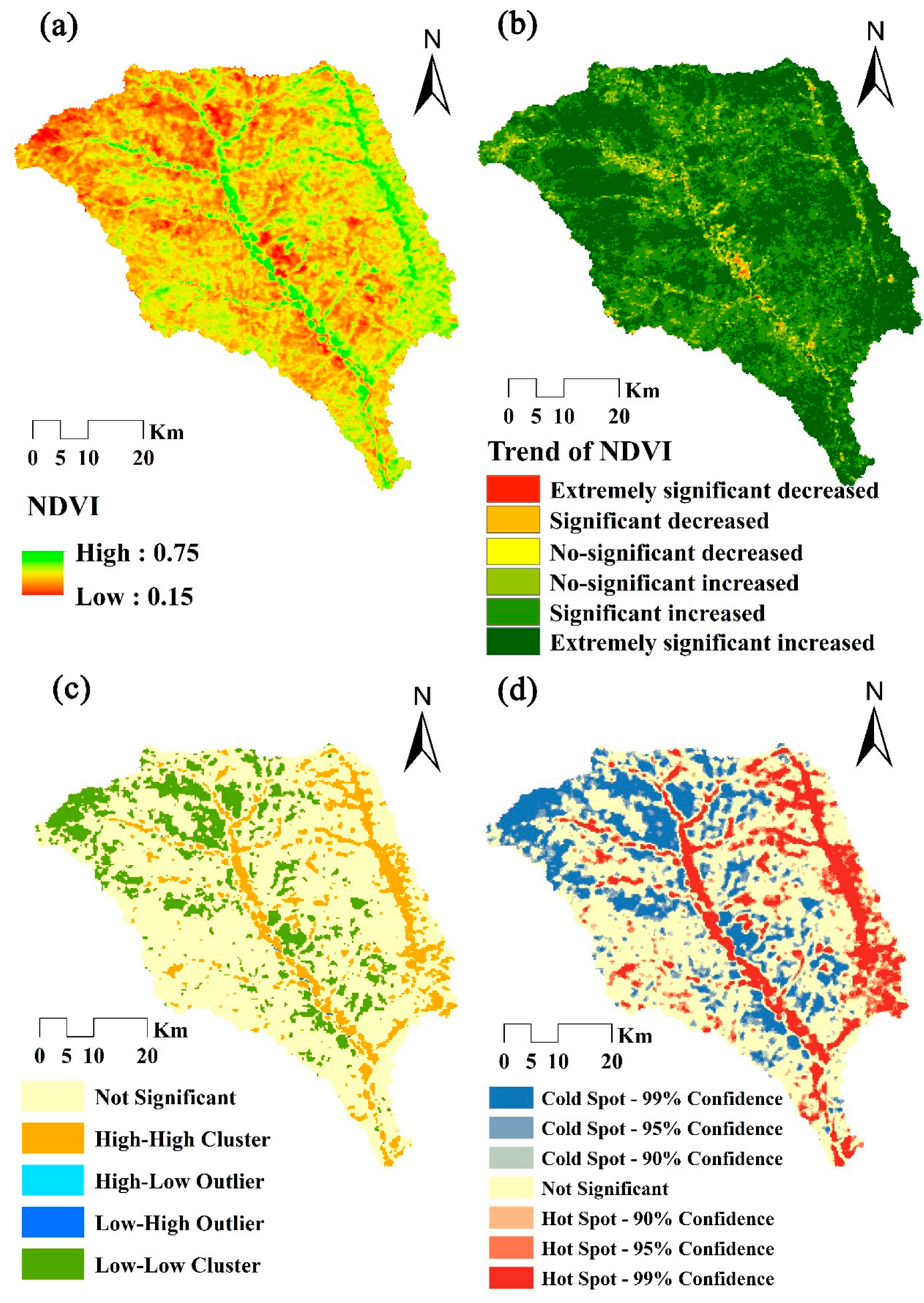
2.2.2. Normalized Difference Vegetation Index

The Normalized Difference Vegetation Index (NDVI) is a vegetation index proposed by Deering [30], which can reflect vegetation growth and cover change. It eliminates the influence of atmosphere, has a long time series, large spatial scale, and strong responsiveness to vegetation changes, and is widely used in a wide range of research areas. Its calculation formula is:

$$NDVI=\frac{\left(NIR-R\right)}{\left(NIR+R\right)}$$

(2)

where NIR represents the reflectance in the near-infrared band; R is the reflectance of the red light band; the range of NDVI is between −1 and 1. A negative value of NDVI indicates that the ground is covered with clouds, water, snow, and the surface is highly reflective of visible light; NDVI of 0 indicates that there are rocks or bare soil; a positive value of NDVI indicates that the ground is covered with vegetation, and the larger the value, the better the growth of vegetation on the surface.

The NDVI was calculated using the Maximum Value Composites (MVC) method to calculate the annual and monthly vegetation growth conditions. Its calculation formula is:

$$AMNDV{I}_i=MAX\left(MMNDV{I}_i\right)$$

(3)

$$MMNDV{I}_i=MAX\left(NDV{I}_{ij}\right)$$

(4)

where AMNDVI_i is the NDVI value for the i year; MAX (MMNDVI_i) is the annual maximum NDVI value corresponding to the i month; MMNDVI_i represents the NDVI value of month i; MAX (NDVI_ij) is the NDVI value corresponding to the j day of the i month.

Trend analysis was further used to perform a linear regression analysis of the change in NDVI over time to predict the intensity and trend of vegetation change, calculated as follows:

$$Slope=\frac{n{\displaystyle \sum _{i=1}^n(i\times NDV{I}_i)}-{\displaystyle \sum _{i=1}^{n}i}\times {\displaystyle \sum _{i=1}^{n}NDV{I}_i}}{n{\displaystyle \sum _{i=1}^n{i}^2}-{\left({\displaystyle \sum _{i=1}^{n}i}\right)}^2}$$

(5)

where Slope is the slope of the trend, NDVI_i is the mean NDVI of the i year, and n is the length of time. When Slope > 0, NDVI is increasing, and the vegetation growth is good; when Slope = 0, NDVI is basically unchanged, and the vegetation growth is average; when Slope < 0, NDVI is decreasing, and the vegetation is degraded.

2.2.3. Spatial Autocorrelation Analysis

Spatial autocorrelation analysis refers to the spatial correlation between a unit in space and the observations of an element in the surrounding units [31,32]. Spatial autocorrelation analysis includes global correlation analysis and local correlation analysis. Global spatial autocorrelation can reveal the overall spatial association and significance of differences in the region, and test whether the observations of spatial units in the global area appear to be clustered, expressed by the statistic Global Moran I [33]; local spatial autocorrelation can indicate the degree of clustering of spatial units in the local area, expressed by the statistic Local Moran I [34], which is calculated as follows:

$$Global Moran I=\frac{n{\displaystyle \sum _{i=1}^n{\displaystyle \sum _{j=1}^n{W}_{ij}\left(x_i-\overline{x}\right)}}\left(x_j-\overline{x}\right)}{{\displaystyle \sum _{i=1}^n{\left(x_i-\overline{x}\right)}^2}{\displaystyle \sum _{i=1}^n{\displaystyle \sum _{j=1}^n{W}_{ij}}}},i\ne j$$

(6)

$$Local Moran I=\frac{\left(x_i-\overline{x}\right){\displaystyle \sum _{j=1}^m{W}_{ij}\left(x_j-\overline{x}\right)}}{{\displaystyle \sum _{i=1}^m{\left(x_i-\overline{x}\right)}^2}},i\ne j$$

(7)

where n is the total number of cells in the region, m is the number of cells adjacent to cell i, x_i, x_j are observations, $\overline{x}$ is the mean value, and w_ij is the spatial cell weight.

The values of Global Moran I range from −1 to 1. I > 0 indicates the existence of positive spatial correlation, and the larger the absolute value indicates greater correlation and more obvious clustering of observations in space; I < 0 indicates the existence of negative spatial correlation, and the larger the absolute value indicates greater heterogeneity and more obvious dispersion of observations in space; I = 0 indicates that the spatial relationship is not obvious and the observations are randomly distributed in space.

Local Moran I results can generate LISA significance level clustering maps, which are divided into five spatial distribution types, namely high-high cluster, low-low cluster, high-low outlier, low-high outlier, and not significant; at the same time, the local spatial aggregation significance is analyzed as cold and hot spots, so as to determine the local spatial “cold spots” and “hot spot”.

2.3. Modeling Strategy

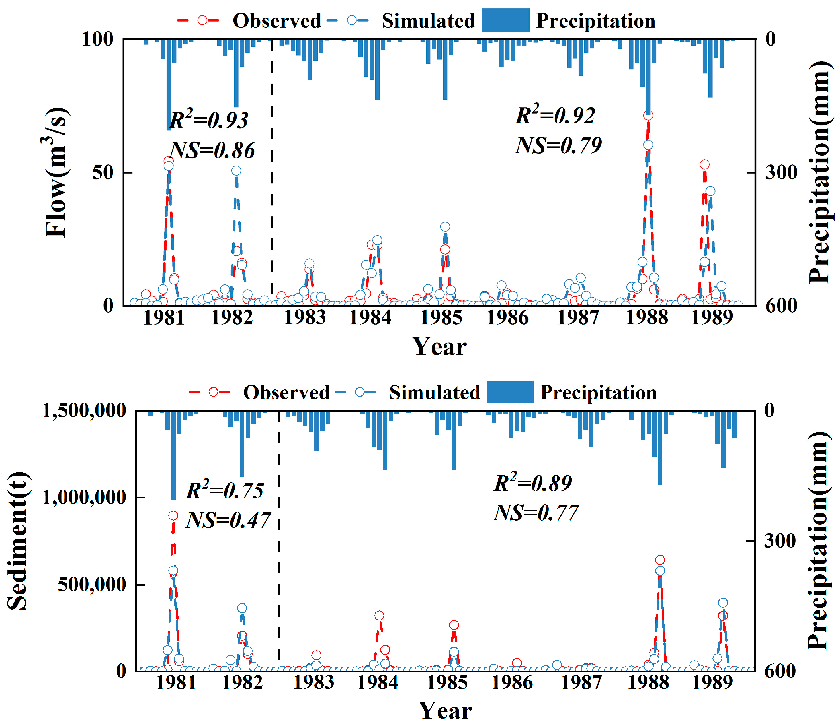
2.3.1. SWAT Model

The SWAT model is a half-distributed hydrological model based on physical mechanisms developed by the United States Department of Agriculture (USDA) Agricultural Research Service [35]. In this study, the Soil Conservation Service Curve Number (SCS-CN) runoff equation [36,37,38] was used to estimate runoff for various land-uses and soil types and is expressed as:

$$Q_{surf}=\frac{{\left(R_{day}-I_a\right)}^2}{\left(R_{day}-I_a+s\right)}$$

(8)

where Q_surf represents cumulative runoff or over-osmotic rainfall, mm; R_day represents daily rain depth, mm; I_a represents the initial water loss, including the ground filling amount, plant interception amount, and infiltration amount before runoff generation, mm; and S represents the retention parameter, mm, varying with soil, land-use, management measures, and slope.

Universal Soil Loss Equation (USLE) [39,40,41] was used to calculate the sediment yield in the sub-basin and is expressed as:

$$Y_{sed}=11.8{\left(Q_{surf}\times q_{peak}\times are{a}_{hru}\right)}^{0.56}{K}_{USLE}\times C_{USLE}\times P_{USLE}\times L{S}_{USLE}\times CFGR$$

(9)

where Y_sed is the sediment yield; Q_surf is the surface runoff; q_peak is the peak discharge; area_hru is the area of the hydrologic research unit; K_USLE is the soil erodibility factor; C_USLE is the land cover and management measuring factor; P_USLE is the soil and water conservation factor; LS_USLE is the topographic factor; and CFGR is the coarseness factor. Note that C_USLE varies according to different plant growth stages:

$$C_{USLE}=\exp \left\{\left[\ln \left(0.8\right)-\ln \left(C_{USLE,mn}\right)\right]\times \exp \left(-0.00115rs{d}_{surf}\right)+\ln \left(C_{USLE,mn}\right)\right\}$$

(10)

C_USLE,mn represents the minimum value of land cover and management measures for the land cover, and rsd_surf represents the amount of residue on the ground.

Organic nitrogen is adsorbed on soil particles and migrates to the main river channel of a watershed along with surface runoff. This form of nitrogen is related to sediment transport in hydrologic research units (HRUs) [42,43], so the organic nitrogen content can reflect the change of sediment transport. The calculation of organic phosphorus is the same as that of organic nitrogen. Organic nitrogen loss can be calculated by the following equation:

$$org{N}_{surf}=0.001con{c}_{orgN}\times \frac{sed}{are{a}_{hru}}\times {\epsilon }_{N:sed}$$

(11)

where orgN_surf represents the amount of organic nitrogen that migrates to the main river channel with surface runoff; conc_orgN represents the concentration of organic nitrogen in the 10 mm soil layer; sed represents the sediment yield for one day; area_hru represents the area of HRU; and ${\epsilon }_{N:sed}$ represents the enrichment ratio of organic nitrogen.

SWAT-CUP was used for parameter calibration and verification [44,45]. The determination coefficient (R²) and Nash efficiency coefficient (NSE) were used to evaluate the simulation effect of the model during the calibration and verification process [46,47,48,49]. The evaluation criterion matched a perfect performance rating to 1, and the closer the value to 1 the better the performance rating. The formulas are as follows:

$$R^2=\frac{{\left[\sum \left(Q_{m,i}-{\overline{Q}}_m\right)\left(Q_{s,i}-{\overline{Q}}_s\right)\right]}^2}{\sum \left(Q_{m,i}-{\overline{Q}}_m\right){\left(Q_{s,i}-{\overline{Q}}_s\right)}^2}$$

(12)

$$NSE=1-\frac{\sum {\left(Q_{m,i}-Q_{s,i}\right)}^2}{\sum {\left(Q_{m,i}-{\overline{Q}}_m\right)}^2}$$

(13)

where Q_m is the observed value of runoff and sediment; Q_s is the simulated value of runoff and sediment; ${\overline{Q}}_m$ is the mean value of observed values; and ${\overline{Q}}_s$ is the mean value of simulated values. The units for the above indicators are m³/s or t.

2.3.2. The EPIC Model

The EPIC model is a dynamic model developed by the Black Soil Research Center of the University of Texas and the US Department of Agriculture to assess the impact of management strategy changes on soil erosion and land productivity [50]. The model is widely used in studies that cover a range of subjects, including crop growth and yield, irrigation, nutrient cycling and losses, wind and water erosion, and soil moisture and temperature regimes [51,52,53]. The EPIC model sets the conditions of climate, soil, topography, crop rotation, and field management measurements in the field area as homogeneous and uses the daily timescale to simulate the growth of crops for a period of time, so as to obtain the dynamic changes of water and soil resources and biomass [54,55,56]. Crop yield estimation is one of the most important applications of the EPIC model, and it can evaluate the potential yield of crops [57,58,59]. This study focuses on the effects of water and nutrient stress on potential biomass in order to further explore the relationship between vegetation and soil erosion.

In the model, plant growth is mainly affected by water stress, temperature stress, nitrogen stress, and phosphorus stress. When any stress occurs during plant growth, the potential biomass growth is calculated in terms of:

$$∆B=\left(∆B_p\right)\left(REG\right)$$

(14)

where $∆B$ is the potential growth of daily biomass, and REG is the crop growth regulating factor (the minimum stress factor).

Water stress (WS) is calculated based on the relationship between water supply and demand during plant growth:

$$W{S}_i={\displaystyle \sum }_{i=1}^M{u}_{i,l}/E_{pi}$$

(15)

where WS_i is the water stress factor of the first day; u_{i, l} is the water use in layer l; and E_pi is the potential water use efficiency of plants on the first day.

Nitrogen stress is calculated as follows, and phosphorus stress is calculated in the same way as N stress.

$$S{N}_i=\frac{S{N}_{s,i}}{S{N}_{s,i}+exp\left(3.52-0.026S{N}_{s,i}\right)}$$

(16)

$$S{N}_{s,i}=200\left(\frac{UN}{{\left(C_{NB}\right)}_i{\left(B\right)}_i}-0.5\right)$$

(17)

where SN_i is the nitrogen stress factor of the first day, UN is the amount of nitrogen absorbed by the plants, C_NB is the optimum nitrogen concentration of the plants, and B is biomass.

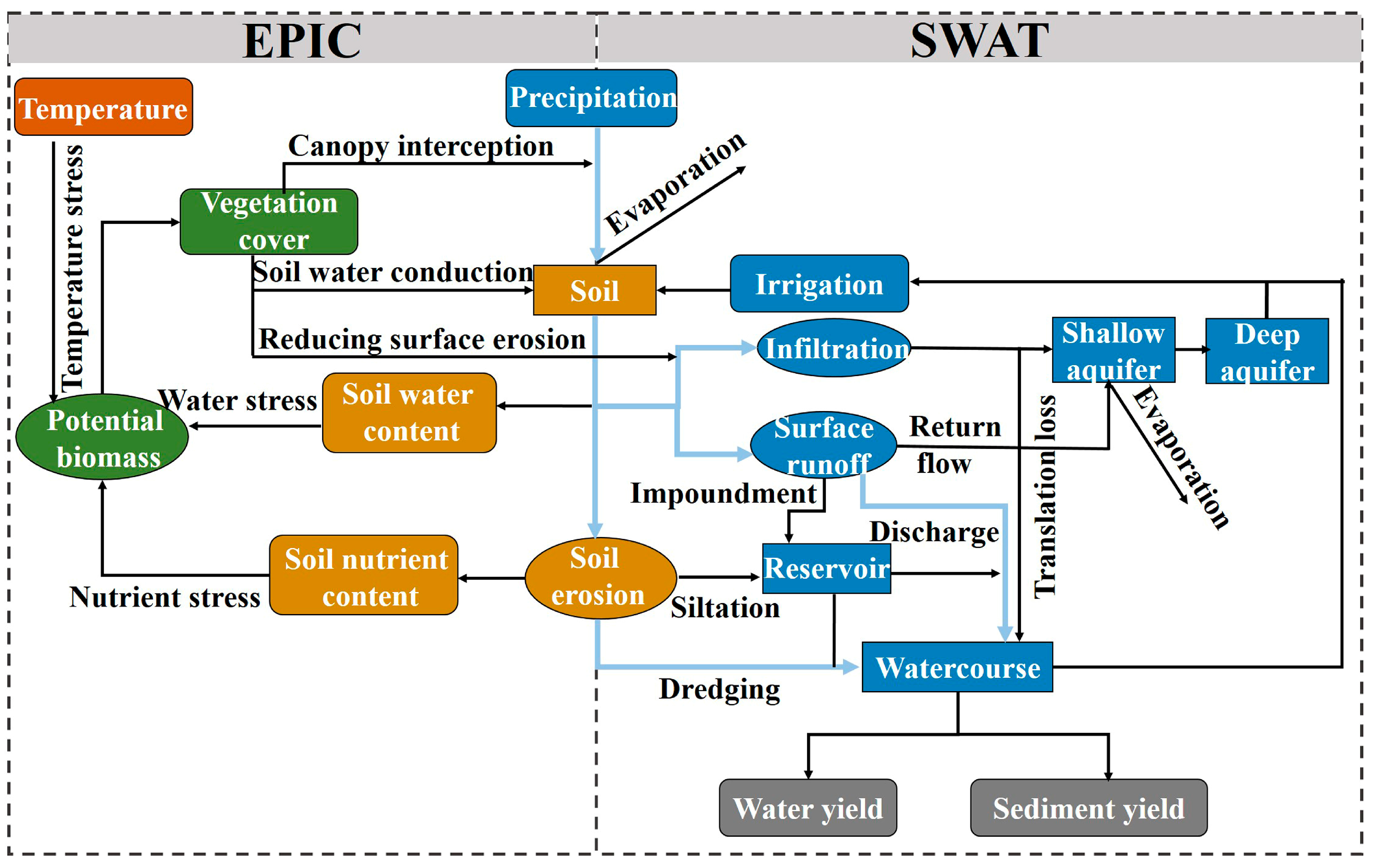
2.3.3. The Comprehensive SWAT-EPIC Framework

Figure 2 shows the structural diagram of the coupled SWAT-EPIC model. Since both EPIC and SWAT were developed at Texas A&M University (TAMU) with the support of the USDA, both systems contain similar modules (e.g., meteorological and soil modules) for certain physical processes [60]. The two models are homogeneous scale models, so a coupled “output-input” model can be established, and the output results of the SWAT model can be input to the EPIC model for simulation after data processing. The SWAT model mainly simulates the process of rainfall erosion flow production and sand production under different land-use situations as a way to investigate the role of vegetation cover on soil erosion. Under the action of precipitation, surface runoff, and subsurface runoff, soil and its components are destroyed, eroded, transported, and deposited and considered as sand production, and nutrients such as nitrogen and phosphorus are transported and lost with particulate matter. The data of the three environmental stress factors—soil water content, soil nitrogen content, and soil phosphorus content—output from the SWAT model were input into the EPIC crop growth module. With other environmental factors in the plant growth database unchanged, two vegetation types, forest and grassland, were selected to simulate their potential biomass under different erosion intensities using their factors such as potential radiation use efficiency and normal harvest index as default universal values. Then, the effect of soil erosion on vegetation growth was explored.

Since the EPIC model is a one-dimensional field-scale model in space, it is difficult to allocate the surface runoff formed by precipitation, resulting in uneven distribution and migration of soil moisture. This leads to unsatisfactory results for the crop yield simulation. Therefore, coupled with the SWAT-distributed hydrological model based on physical processes such as runoff yield and confluence, the hydrological processes like soil erosion, sediment yield, and sediment transport can be calculated with climate, topography, soil vegetation, and other factors taken into consideration so that the simulation process is closer to reality.

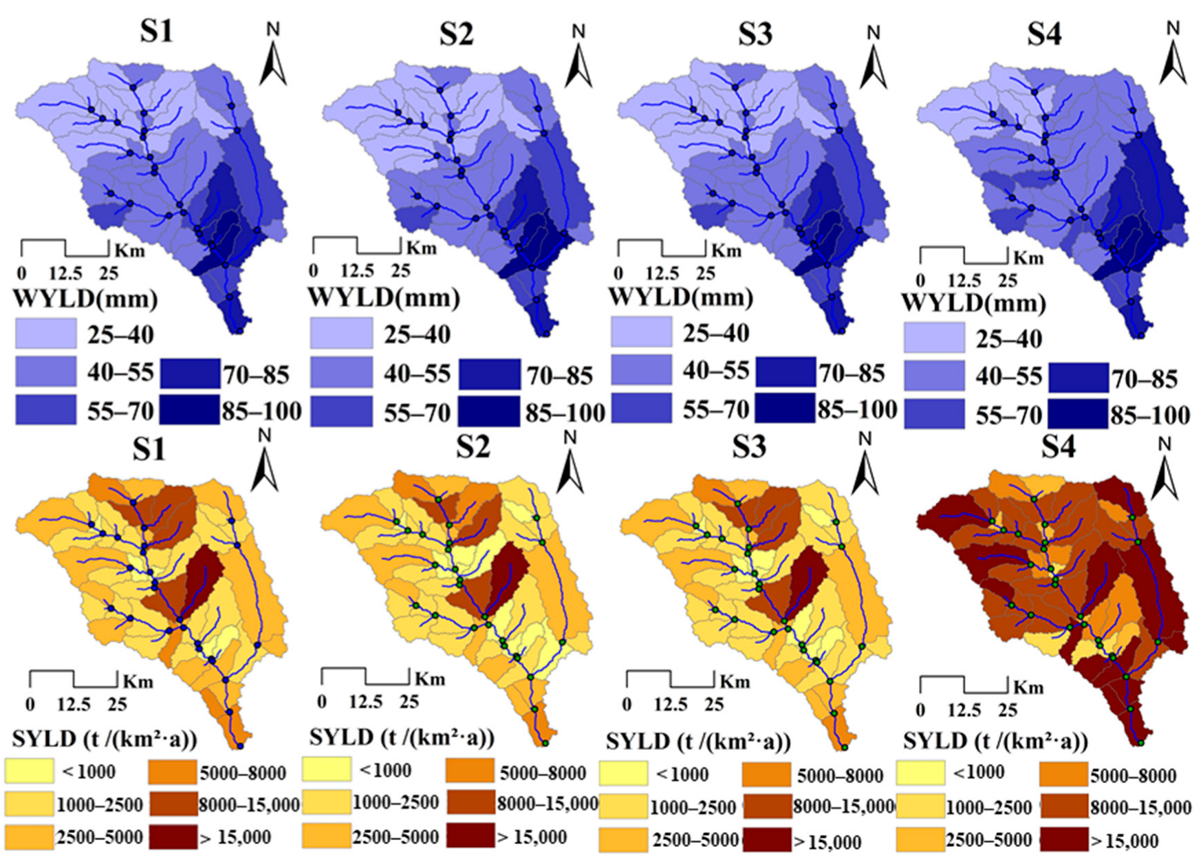
2.4. Simulation Scenarios

Land-use and land cover change are some of the primary factors causing soil erosion, which affects the redistribution and operation of water and changes the hydrological cycle, water balance, and hydrological characteristic values of the watershed [61]. Land-use changes in vulnerable erosion-prone areas have long-term effects on hydrological processes [62]. Variations of river runoff and sediment discharges driven by land-use and land cover change were evaluated by scenario simulations using SWAT modeling. Taking the outputs of SWAT as the input conditions for the EPIC model, the effects of soil and water loss on vegetation coverage were further assessed in this study.

Four different scenarios were set as follows: the 1984 land-use map was used as the base period scenario (S1), while the grassland cover scenario (S2) was set as converted cultivated land into grassland, and the difference in runoff and sediment discharge between S2 and S1were considered to be caused by grassland. The forest land cover scenario (S3) was set as convert cultivated land into forest, and the variations of runoff and sediment discharge between S3 and S1 were considered to be caused by forest change. The bare land cover scenario (S4) was set as the conversion of cultivated land to bare land, and the difference in the amount of watershed erosion that changed between S4 and S1 was assumed to be caused by bare land.

The base period scenario (S1): the cultivated land, grassland, forest, urban land, water, and bare land in the simulation area remain unchanged.

The grassland cover scenario (S2): the forest, urban land, water, and bare land in the simulation area were kept unchanged, and all cultivated land was set as grassland. At this time, the grassland coverage in the simulation area was 87.46%.

The forest land cover scenario (S3): the grassland, urban land, water, and bare land in the simulation area were kept unchanged, and all cultivated land was set as forest. At this time, the forest coverage in the simulation area was 26.22%.

The bare land cover scenario (S4): the forest, grassland, water, and bare land in the simulation area were kept unchanged, and all cultivated land was set as bare land. At this time, the bare land coverage in the simulation area was 26.47%.

3. Results

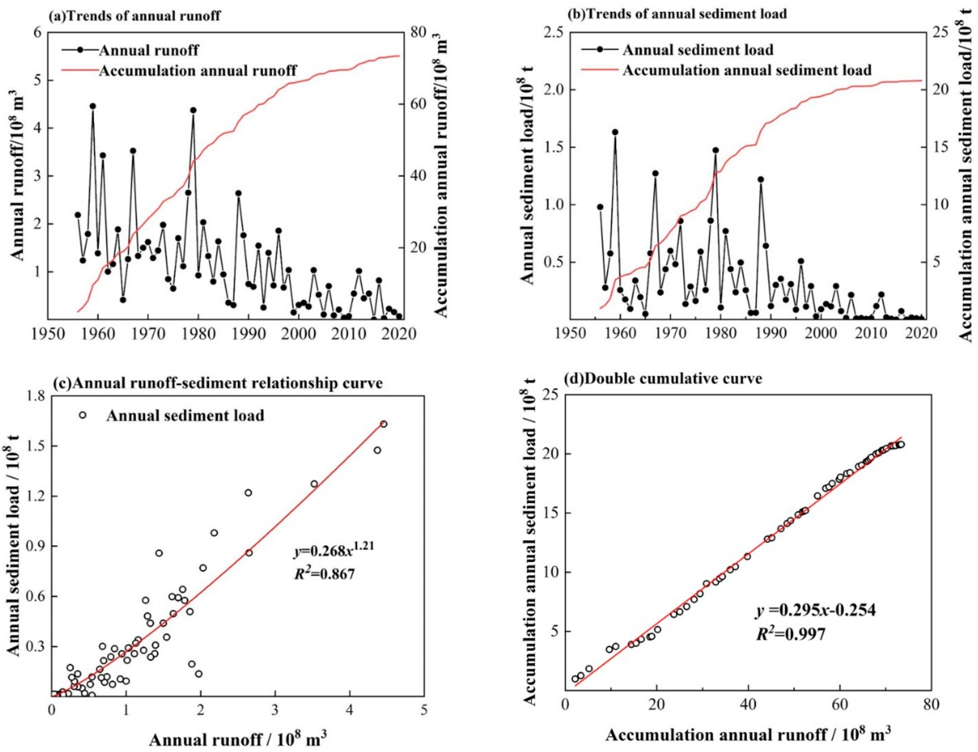
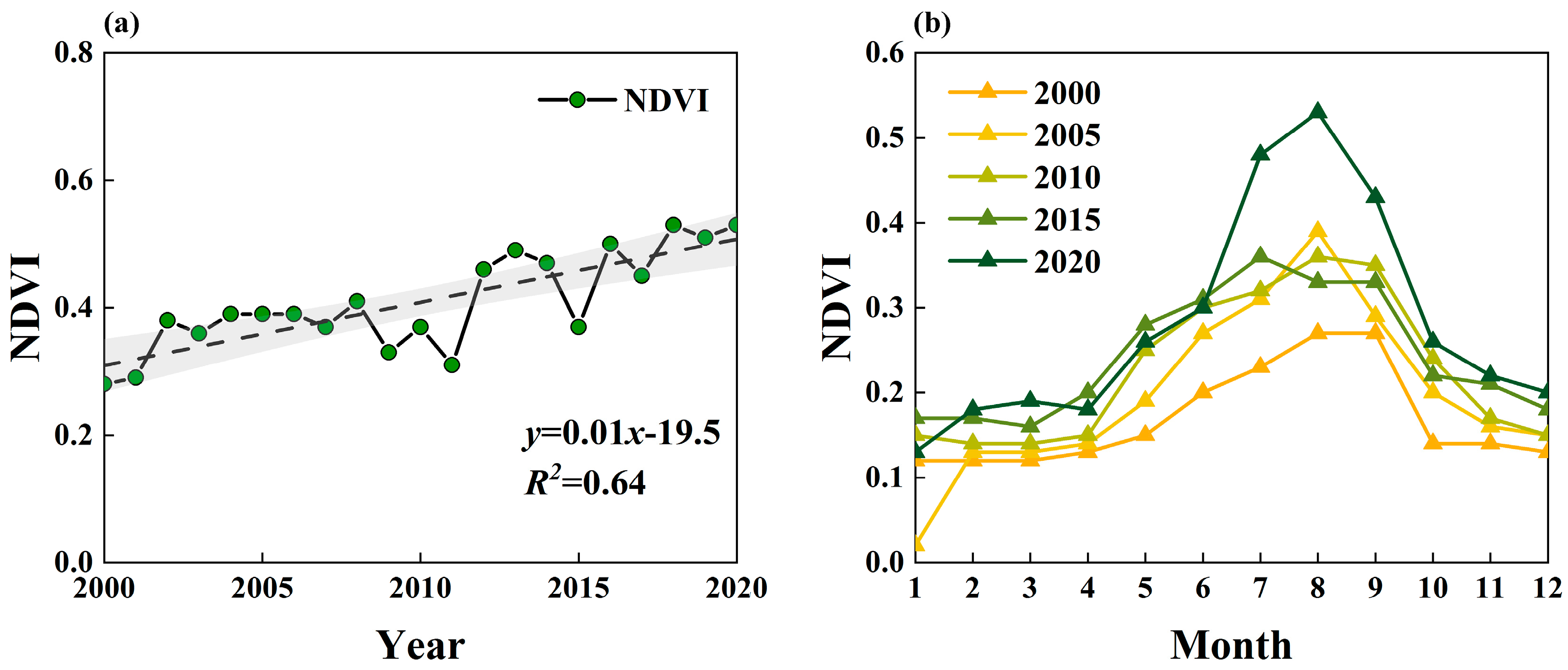
3.1. Variations in the Water-Sediment Relationship and Vegetation

The variation trend of annual runoff and annual sediment load in the Huangfuchuan Watershed from 1956 to 2020 is shown in Figure 3a,b. From 1956 to 2020, the average annual natural runoff was 113 million m³, and the average annual sediment load was 0.32 million tons. The runoff showed a fluctuating downward trend, and the reduction rate was 32.5 million m³ per year. The maximum and minimum values appeared in 1959 and 2015, and the values were 446 million m³ and 0.0005 million m³, respectively. The equivalent runoff depths were 1.48 × 10⁵ mm and 16.98 mm, respectively. The change of sediment load was similar to that of runoff and showed a significant decreasing trend, with a decreasing rate of about 15 million t per year. The maximum and minimum values appeared in 1959 and 2015 and were 1.63 × 10⁸ t and 55.1 t, respectively. The equivalent erosion modulus was 5.2 × 10⁻⁴ t/(km²·a) and 1.7 × 10⁻² t/(km²·a), respectively.

Figure 3c presents the water-sediment relationship curve for the Huangfuchuan Watershed from 1956 to 2020. The water-sediment relationship conforms to the power function relationship; the determination coefficient is 0.867, and the fitting effect is good. Each correlation point is distributed near the water-sediment relationship curve, and there is no systematic deviation. Most of the relevant points are concentrated in the range of annual runoff less than 200 million m³, and a small part is dispersed in the range of annual runoff of more than 200 million m³. In the water-sediment relationship curve, the factor representing the external influence is 0.268, and the factor representing the sediment transport energy of the river is 1.21.

The double accumulation curve is plotted in Figure 3d, in which the annual cumulative runoff is used as the scale point and the annual cumulative sediment load is used as the ordinate. It can be seen that the double accumulation curve is basically a straight line with a gradual decrease in sand production. From the 1950s to the 1970s, local governments began to adopt afforestation, terracing, and silt dam construction projects to control slope erosion. From the 1980s to the 1990s, small watershed management and protective forest construction were mainly carried out to control slope-gully erosion to intercept sediment and improve the ecological environment. Since 2000, the project of returning farmland to forests (grass) has been carried out, focusing on biological management methods to improve the ecological environment and reduce soil erosion. In 2016, the Loess Plateau was designated to be in the first batch of study areas for the Ecological Protection and Restoration Project for Mountains, Rivers, Forests, Fields, Lakes, and Grasses. Now, the management of soil erosion on the Loess Plateau has entered a new stage, and soil erosion in the watershed has been effectively controlled.

Figure 4 shows the trend of inter-annual and intra-annual variation of NDVI in the Huangfuchuan Watershed from 2000 to 2020. The inter-annual scale NDVI of Huangfuchuan Watershed shows an increasing trend, from 0.28 in 2000 to 0.53 in 2020. Since the Loess Plateau started to implement the policy of returning farmland to forests and grasses in 1999, the vegetation cover has increased annually, soil erosion has been effectively controlled, water and soil loss have been effectively managed, and the ecological environment has been well improved. The analysis of intra-annual NDVI in 2000, 2005, 2010, 2015, and 2020 showed that NDVI started to increase in April, when plants started to grow, then NDVI values peaked in August and vegetation cover reached its maximum, then NDVI values started to decline and vegetation started to die off.

Figure 5a shows the spatial distribution of multi-year average NDVI in the Huangfuchuan Watershed from 2000 to 2020, with NDVI values ranging from 0.15 to 0.75, spatially showing high values in the gully and low values in the slope, as well as high values in the southeast and low values in the northwest. The analysis of NDVI trend (Figure 5b) shows that 49.65% of the area of Huangfuchuan Watershed was highly significantly improved, 42.47% was significantly improved, and 6.6% was not significantly improved, and the overall area showed more improvement and less degradation.

Spatial autocorrelation analysis of NDVI in the Huangfuchuan Watershed indicated that the global Moran’s I index of NDVI from 2000 to 2020 was 0.796, with Z-value greater than 2.58 and P-value less than 0.01, showing a significant positive spatial autocorrelation and NDVI was aggregated. In order to investigate the local spatial aggregation characteristics of NDVI in the study area, local spatial autocorrelation analysis was conducted. Figure 5c shows that the non-significant area is large, the “high-high” cluster area is mainly concentrated in the two tributary channels, which indicates that the vegetation cover is better, and the “low-low” cluster area is distributed in the northwest and central part of the study area. The spatial anomalies “low-high” outlier and “high-low” outlier are relatively few, indicating that there are fewer extreme values of NDVI in the Huangfuchuan Watershed. The spatial distribution characteristics and evolution trend of NDVI in Huangfuchuan Watershed were investigated by hot spot analysis. Figure 5d showed that the hot spots of NDVI were concentrated near the two tributary channels, and the cold spots of NDVI were in the southwest and central part of the basin.

The land-use cover change of the Huangfuchuan Watershed from 1985 to 2020 showed a decrease in cropland area and an increase in forest and grassland areas. The land-use maps shown in Figure 6 cropland area decreased from 23.06% to 11.51%, forest area increased from 0.02% to 0.03%, and grassland area increased from 73.09% to 85.87%. Land-use changes are clearly related to government policy changes. The Huangfuchuan Watershed experienced comprehensive attention related to governmental policies since 1984. Through the small watershed comprehensive management project, after years of comprehensive soil and water conservation management, the ecological restoration of the watershed has been effective. Since the implementation of the “Returning Farmland to Forestry and Grassland” project in 1999, the cultivated land area decreased, the forest land and grassland areas increased, and the ecological environment has been greatly improved. With the continuous improvement of ecological and economic benefits, some farmers voluntarily moved into cities. Urbanization and economic development also promoted the dramatic expansion of urban land, which increased from 1.60% to 2.46%. The water area increased by 18.75%, which had a slight advantage on future vegetation restoration and agricultural production in the watershed.

The transition matrix of land-use changes in

Table 1. Transition matrix of land-use changes in the Huangfuchuan Watershed from 1985 to 2020.

		2020
		Cropland	Forest	Grassland	Water	Urban Land	Bare Land	Total
1985	Cropland	286.27	0.00	454.01	0.54	7.74	0.00	748.56
	Forest	0.00	0.54	0.00	0.00	0.00	0.00	0.54
	Grassland	84.35	0.54	2266.95	0.75	18.27	1.61	2372.47
	Water	1.07	0.00	0.21	0.43	0.00	0.00	1.72
	Urban land	0.11	0.00	0.00	0.32	51.58	0.00	52.01
	Bare land	1.93	0.00	66.19	0.00	2.26	0.32	70.70
	Total	373.74	1.07	2787.36	2.04	79.84	1.93	3245.99

shows detailed changes in the Huangfuchuan Watershed from 1985 to 2020. From the changes of land-use types, the large amount of cultivated land converted to grassland reflects the importance of the “Returning Farmland to Forestry and Grassland” policy, and the most effective treatment for soil erosion is planting grass. Additionally, most of the bare land was converted to grassland, indicating that the region attaches importance to the greening of bare land. Urban land expansion has occurred mainly through the occupation of cultivated land and grassland, and it shows that the locals choose either returned farmland or grassland to use as urban land. The increase of water area indicates that with the increase of forest and grass areas, the water conservation capacity is improved, which is conducive to improving the value function of ecological resources.

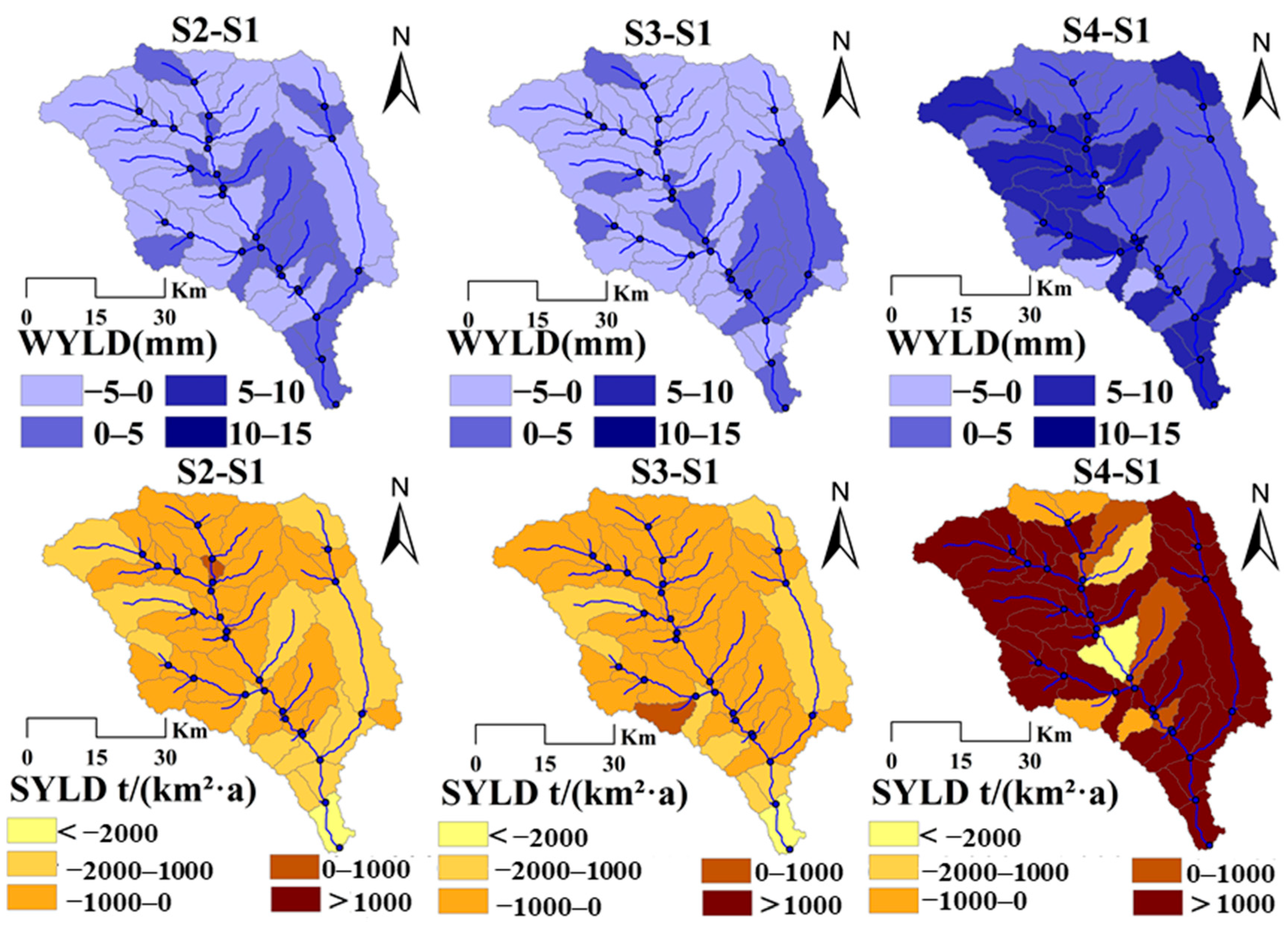
3.2. Effects of Vegetation Changes on Erosion

In order to explore the impact of vegetation changes on erosion, this study used the SWAT hydrological model to simulate four land-use patterns for the base period (S1), a grassland cover scenario (S2), a forest cover scenario (S3), and a bare land cover scenario (S4). Specifically, we explored the water and sediment yield so as to provide a reference for the adjustment of land-use in the Huangfuchuan Watershed.

Sensitivity analysis was primarily performed before scenario simulations. This study used 13 parameters related to runoff and sediment to perform the sensitivity analysis (

Table 2. Runoff and sediment load sensitive parameters in the Huangfuchuan Watershed.

Parameter Acronym	Parameters	Range	Optimum Value	Rank
V CANMX	Maximum canopy storage	(0, 100)	44.167	1
V SOL_K	Saturated hydraulic conductivity (mm/hr)	(0, 2000)	856.667	2
V GWQMN	Threshold depth of water in the shallow aquifer return flow to occur (mm)	(0, 5000)	4675	3
V GW_DELAY	Delay time of groundwater supply flow	(0, 500)	144.167	4
V ESCO	Compensation factor for evaporation from soil	(0, 1)	0.468	5
V ALPHA_BF	Groundwater reaction factor	(0, 1)	0.778	6
R CN2	Curve number	(−1, 1)	0.193	7
V USLE_P	Factor related to soil conservation operations in the USLE equation	(0, 1)	0.112	8
V SPEXP	Exponential re-entrainment coefficient for channel sediment routing sediment added in river sediment calculation	(1, 1.5)	1.006	9
V GW_REVAP	Groundwater “revap” coefficient	(0.02, 0.2)	0.116	10
V SPCON	linear parameter for calculating the maximum amount of sediment that can be reentrained during channel sediment routing sediment added in river sediment calculation	(0.0001, 0.01)	0.009	11
V USLE_K	USLE equation soil erodibility (K) factor	(0, 0.65)	0.075	12
V SOL_AWC	Available water capacity in the soil layer	(0, 1)	0.341	13

). The simulation period of the SWAT model was divided into a calibration period and a verification period. During the calibration period, the simulation effect was optimized by adjusting the sensitivity parameters of the model. The verification period involved using the adjusted parameters to run the model and comparing results with observed values to verify the simulation effect of the model. Monthly runoff and sediment transport data from the Huangfu hydrological station in the Huangfuchuan Watershed from 1981 to 1989 were used for simulation due to the integrity of the measured meteorological data and hydrological station runoff data at this location. The preheating period was from 1978 to 1980; the calibration period was from 1981 to 1982; and the verification period was from 1983 to 1989. The purpose of setting the preheating period was to avoid the influence of the parameter value of 0 in the early stage of the model operation. Figure 7 shows the comparison results between the simulated and observed values at the monthly scale of the model in the calibration period and verification period. Statistical performance metrics such as R² and NSE show that the results of the SWAT modeling are satisfactory.

Table 3. Simulation results for average annual water yield and sediment yield for four scenarios.

Scenario	Water Yield (mm)			Erosion Modulus (t/(km2·a)).
	Average	Change	Percent	Average	Change	Percent
Base period scenario (S1)	49.17	-	-	3356	-	-
Grass land cover scenario (S2)	48.85	−0.32	−0.65%	2677	−680	−20.24%
Forest cover scenario (S3)	48.87	−0.30	−0.61%	2762	−594	−17.71%
Bare land cover scenario (S4)	54.02	4.85	9.86%	10390	7034	209.60%

shows the quantitative analysis results of vegetation to water yield and sediment yield in Huangfuchuan Watershed under different land-use types. Under the influence of human activities, the impact of land-use on runoff and sediment is different. In terms of runoff, the water yield of S2 was 0.32 mm lower than that of S1, with a decrease of 0.65%. The water yield for S3 was reduced by 0.30 mm compared with S1, and the reduction ratio was 0.61%. The water yield for S4 increased by 4.85 mm compared with that in S1, with an increase of 9.86%. Under the change of total runoff, there are significant differences in the impact of different land-use scenarios on runoff: S2 > S3 > S4. In terms of soil erosion, the sediment yield of S2 decreased by 680 t/(km²·a) compared with S1, and the reduction ratio was 20.24%. The sediment yield of S3 was 594 t/(km²·a), lower than that of S1, and the reduction ratio was 17.71%. It can be seen that grassland has stronger sand retention ability than forest land. This is because the density of herbaceous plants is higher than that of trees, and the denser vegetation better traps sediment. For example, the horizontal root distribution of trees is deep, and densely distributed herbaceous plant roots are usually distributed just below the surface, which is of great significance to effectively prevent the loss of fertile soil from the surface and to prevent shallow gully erosion. The sediment yield of S4 increased by 7034 t/(km²·a) compared with that of S1, with an increase rate of 209.60%. This is due to the bare area being unable to intercept water and sand, eventually leading to increased soil erosion.

Figure 8 reflects the changes of average annual water yield (WYLD) and sediment yield (SYLD) under different scenarios at a spatial scale. The water yields under the four scenarios are within the range of 0–100 mm, showing a decreasing trend from southeast to northwest. In some southwest and central regions, the water yield was higher than 55 mm. Compared with S1, S2 and S3 were basically the same in water yield, and S4 increased slightly in the southeast region. In terms of the sediment yield, using the soil erosion intensity grading scale as a standard, the distributions of S2 and S3 were similar to that of S1, and the erosion modulus was mostly in the range of 0–5000 t/(km²·a). The sediment yield in the northern and southern parts was larger, which is in the range of 5000–8000 t/(km²·a). The middle part was the largest, more than 15,000 t/(km²·a). The erosion amount near the main river channel of the Huangfuchuan River was obviously higher than that around the slope. The sediment yield of S4 was very severe. Except for the southwest region, the erosion modulus in other regions was above 8000 t/(km²·a), and the erosion in the northwest and southern regions and near the Shilichangchuan River was particularly serious, exceeding 15,000 t/(km²·a).

Figure 9 shows the spatial distribution of the difference value of water yield and sediment yield between S2, S3, S4, and S1. In terms of the water yield, most of the decreased values were between 0 and 5 mm under S2. The area near the junction of the Huangfuchuan River and Shilichangchuan River has the largest increase, ranging from 0 mm to 5 mm, and the maximum value added of water yield was 2.34 mm. The difference value of water yield for S4 was basically increased; most areas were 0–5 mm and 5–10 mm, and the added value of the northwest and south parts was more than 10 mm. From the spatial distribution of the difference values in sediment yield, the value between S2 and S1 was basically negative, indicating that soil erosion was significantly reduced. Except for sporadic areas in the south, the variation in other regions was within 2000 t/(km²·a). The erosion reduction in the northern and central parts of the watershed was less than 1000 t/(km²·a), and the erosion of a small part of the area near the river channel showed an increasing trend, with an increase of 0–1000 t/(km²·a). Compared with tS1, sediment yield in the watershed also showed a downward trend in S3, with the largest reduction in the south, exceeding 2000 t/(km²·a); variations in the remaining regions were within 2000 t/(km²·a). Only part of the southwest region showed an increasing trend, with an increase of 0–1000 t/(km²·a). The erosion of S4 was the most serious, and the overall watershed showed an increasing trend, with changes of more than 1000 t/(km²·a) in most areas. The erosion variation in the northwestern and southern regions was huge, over 10,000 t/(km²·a); these two regions have severe erosion.

Deforestation, land clearing, and cultivation on steep slopes are among the important causes of soil erosion on the Loess Plateau. The results achieved by the soil and water conservation measures of the “Returning Cultivated Land to Forests and Grasses” project validate its aim. The S2 was more effective among the four simulation results, probably because the dense grass increased the roughness of the ground, effectively blocking runoff and intercepting sediment. Studies have shown that developing grassland can form a compact root system which loosens the soil and effectively increases water infiltration. In addition, the residual roots left by the grassland bring rich organic matter to the soil, which can increase the aggregated structure of the soil and improve the physical and chemical properties of the soil, thus maintaining water and soil in the grassland. The reason for the occurrence of S3 may be that woodlands can increase infiltration to some extent, improve soil permeability and water holding capacity, and also reduce soil erosion, regulate surface runoff, and protect water resources. The reason for S4 may be that the bare land surface cannot stop the flow of water and sediment, leading to increased water erosion. It can be seen that the “Returning Cultivated Land to Forests and Grasses” project not only prevents wind and sand, but also reduces runoff and serves to reduce flood peaks while carrying out ecological restoration.

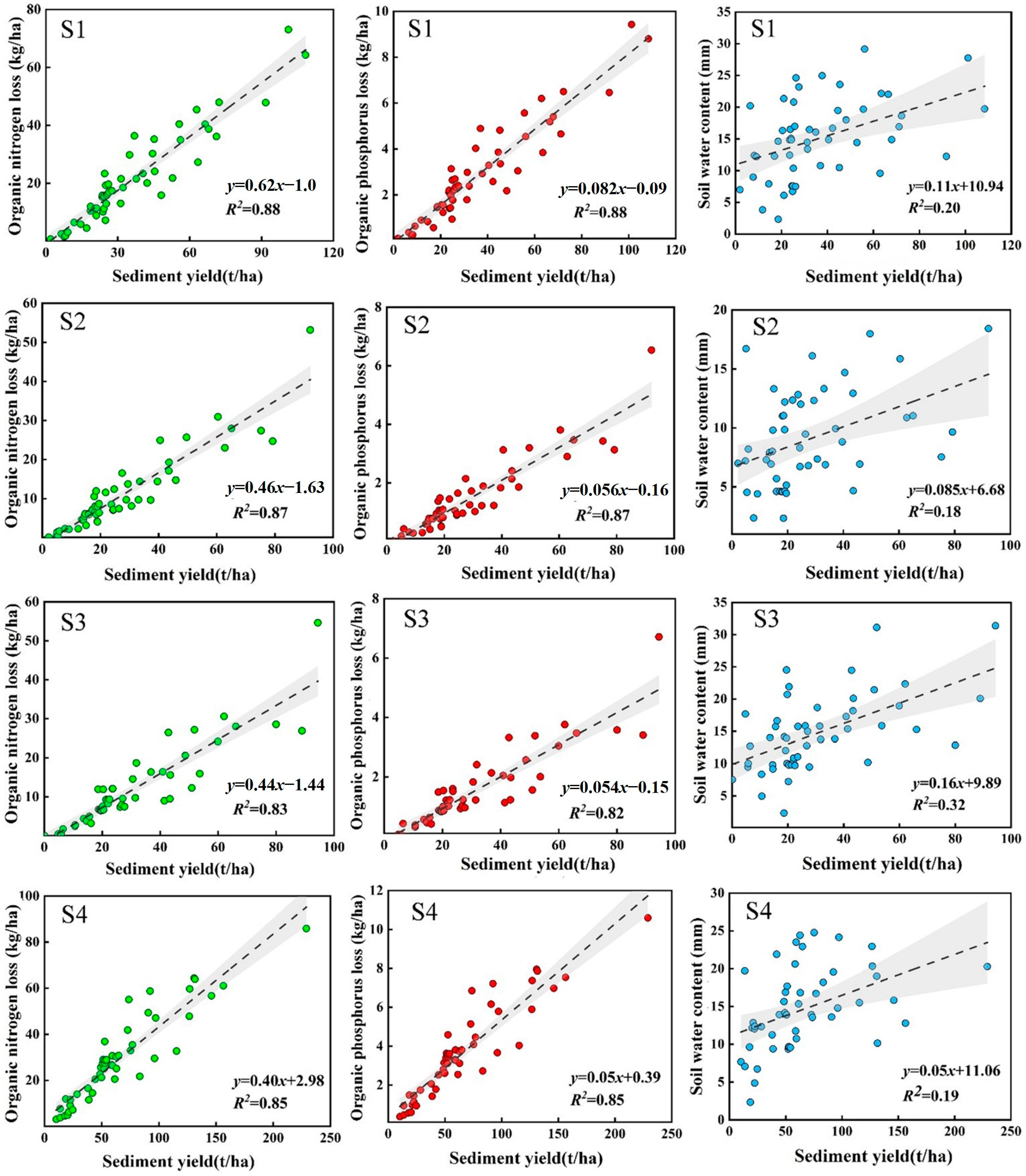
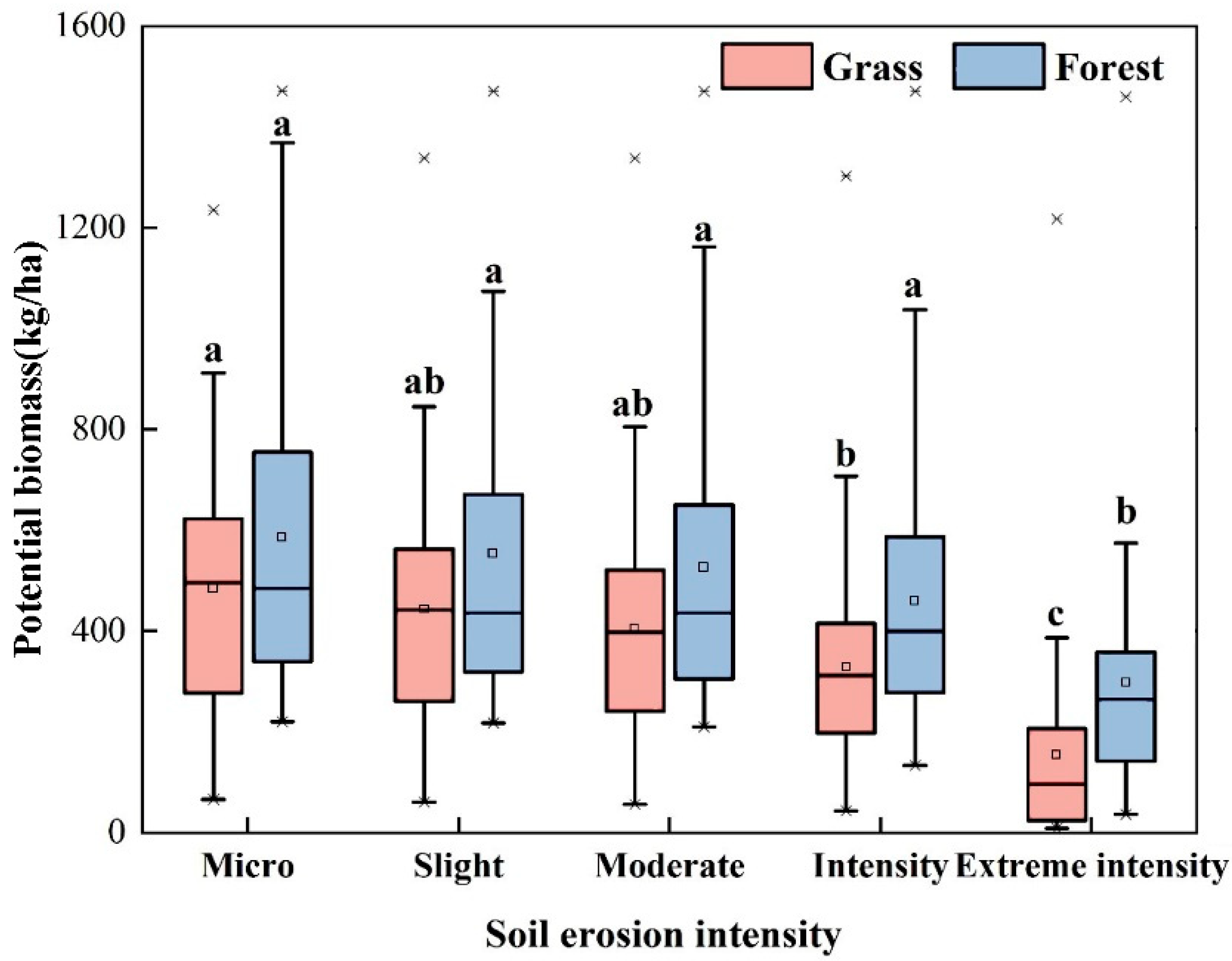
3.3. Effects of Erosion on Vegetation Growth

Long-term soil erosion would lead to high fertile soil particle loss along with water loss, soil nutrient content reduction, and vegetation degradation. Therefore, the primary environmental control factors output by SWAT model (i.e., organic nitrogen, organic phosphorous, and water content) were selected as input stresses for the EPIC vegetation growth model. Figure 10 presents the linear positive correlations between sediment yield and these three factors under four different scenarios.

Nitrogen is one of the most necessary nutrients for plants. Soil nitrogen content is mainly affected by vegetation, climate, soil texture, topography and terrain, tillage and utilization methods, cultivation management, and fertilization measures. In general, under similar climate conditions, soil humus and nitrogen content accumulated by herbaceous vegetation are higher than that accumulated in woody plants. Figure 10 shows that nitrogen loss is linearly correlated with the erosion modulus, and the determination coefficients of S1–S4 are 0.88, 0.87, 0.83, and 0.85, respectively, which means the fitting effect is acceptable, showing a significant upward trend. The correlation points between nitrogen loss and the erosion modulus are mostly distributed near the correlation line, and there is no deviation. With the increase of soil erosion intensity, soil moisture content increases, and nitrogen loss increases, which may be due to the large flow of materials in the erosion process and soil organic nitrogen loss with soil particle migration. Regarding the curve of best fit, when the erosion amount was 0, the loss of S4 was 2.98 kg/ha, indicating that the nitrogen loss in bare land was serious. On the other hand, the nitrogen loss of S1 was −1 kg/ha, S2 was −1.63 kg/ha, and S3 was −1.44 kg/ha, indicating that without erosion, the soil nitrogen content was the highest in grassland, followed by forest, and the lowest was in cultivated land.

Phosphorus is a sedimentary mineral. The content of soil organic phosphorus is mainly affected by soil texture, profile level, soil erosion, and tillage management measures. It can be seen from Figure 10 that phosphorus loss is linearly correlated with the erosion modulus, and the determination coefficients of S1–S4 are 0.88, 0.87, 0.82, and 0.85, respectively. The fitting effect is good, showing a significant upward trend. The change of phosphorus loss and nitrogen loss was basically the same, and the correlation points between phosphorus loss and the erosion modulus are mostly distributed near the correlation line, without deviation. Under micro-erosion, slight erosion, and moderate erosion, phosphorus loss was mostly below 4 kg/ha. With the increase of soil erosion intensity, phosphorus loss increased. When soil erosion occurs, soil moisture is lost, surface runoff increases, phosphorus migrates with large particles, and nutrients are lost. It can be seen from the curve of best fit that the loss of S4 was 0.39 kg/ha when the erosion amount was 0, indicating that bare land soil had difficulty maintaining nutrients, resulting in serious phosphorus loss. The phosphorus loss of S1 was −0.09 kg/ha, S2 was −0.16 kg/ha, and S3 was −0.15 kg/ha, indicating that the soil phosphorus content was the highest in grassland, followed by forest land and cultivated land without erosion, which is consistent with previous results.

With the increase of soil erosion, the soil moisture content also increases. When the erosion amount was 0, the soil water content values compared as follows: S4 > S1 > S3 > S2, indicating that the soil water content of bare land was relatively high. Grassland and forest have less runoff than bare land, but vegetation transpiration consumes more water, evaporation is greater than bare land, and soil water circulation is stronger, so the soil water content of bare land is greater than that of forest and grassland.

As an important feature of the ecosystem, potential biomass can be used to measure the content of biological organic matter, which reflects an ecological community’s productivity and ability to fix solar energy. It is an indispensable index for remote sensing crop yield estimation and ecological environment monitoring, and it plays an important role in the study of soil and water conservation. Different restoration measures change the habitat of degraded ecosystems to different degrees, which directly affect the growth of individual plant species in the community, resulting in differences in potential biomass for different restoration communities. In this study, the SWAT model was used to simulate environmental stress factors, N and P content, and soil water content under different erosion intensities during the reference period (S1). These factors were also put into the EPIC model as a way to evaluate plant growth conditions. Under the same conditions for other environmental factors, the potential biomass of two vegetation types of forest and grass was explored under different erosion intensities and under the condition of “Returning Farmland to Forestry and Grassland”. The EPIC model simulates the dynamic variations of crop leaf area driven by meteorological data under different erosion intensities, and then calculates photosynthetically active radiation. Forest and grass were selected as vegetation types, and no fertilizer and pesticides were considered during the simulation. The potential growth biomass was calculated by the relationship between photosynthetically active radiation and light use efficiency. Then, considering the effects of water stress, temperature stress, and nitrogen and phosphorus nutrition stress on vegetation biomass and leaf area, the potential vegetation growth biomass was calculated. Environmental parameters in the EPIC model are shown in

Table 4. Environment parameters in the EPIC model.

Soil Erosion Intensity	Soil Water Storage (Fraction of Field Capacity)	Organic Nitrogen (kg/ha)	Organic Phosphorus (kg/ha)
Micro	0.25	99.24	24.89
Slight	0.53	88.78	23.56
Moderate	0.58	81.48	22.62
Intensity	0.60	63.87	20.35
Extreme intensity	0.98	26.94	15.58

.

Figure 11 shows the potential biomass of forest and grassland under different erosion intensities from 1984 to 2020. Under micro-erosion, the annual average potential biomass of forest land was 585.7 kg/ha, and that of grassland was 485.9 kg/ha. With the increase of erosion intensity, the biomass of forest and grassland decreased. Under extremely intense erosion, the annual average potential biomasses of forest and grass were 297.9 kg/ha and 154.6 kg/ha, respectively. Compared to the micro-erosion condition, the average annual potential biomass of forest was reduced by half, while the average annual potential biomass of grassland was reduced by two-thirds. The results presented that the vegetation potential biomass was the largest under micro-erosion conditions, while it decreased sharply under extremely intense erosion conditions. It is notable that the potential biomass of the forest had less of a decreasing trend than that of the grassland, indicating that biomass of forest is less affected by soil erosion and thus presented better stability to environmental change than that of the grassland.

4. Discussion

4.1. Runoff and Sediment Reduction by Vegetation

The influence of vegetation on the water yield mainly affects four levels, namely vegetation canopy [63,64], the shallow soil layer [65,66], the deep soil layer [67,68], and the groundwater aquifer [69,70]. The relationship between different vegetation types and soil erosion also varies. The soil and water conservation functions of forests are improved by vegetative cover and plant root systems, which increase water interception and infiltration, and decrease runoff and soil erosion. Grassland directly intercepts sediment through the surface vegetative canopies [71,72]. The water yield is also related to plant morphology and canopy cover, and a dry soil layer with dense plant cover can also improve hydraulic conductivity and decrease raindrop force and sealing [73,74]. The results show that among the parameters affecting runoff, maximum canopy storage (CANMX) is the most sensitive, reflecting the interception ability of vegetation to rainfall in the process of the hydrological cycle. The larger the vegetation coverage, the larger the canopy rainfall capacity of the ecological community. Large vegetation coverage means a denser distribution of vegetation, and the larger the canopy interception range of rainfall, the more rainfall is intercepted and runoff is reduced [75]. The main land-use types in the Huangfuchuan Watershed are grassland, cultivated land, and forest. Grassland is the largest land-use type in the watershed, accounting for 65.86% of the total area, followed by cultivated land, accounting for about 20.99%, and forest area, accounting for 5.26%. The second sensitive parameter is saturated hydraulic conductivity (SOL_K). It relates the soil water flow rate to the hydraulic gradient and is a measure of the ease of water movement through the soil. K is the reciprocal of the resistance of the soil matrix to water flow; it is an important parameter reflecting soil infiltration characteristics. Soil moisture is a fundamental limiting factor for plant growth and vegetation restoration in the Loess Plateau. The annual rainfall in the Loess Plateau is concentrated and the rainfall is heavy. Therefore, the water storage function of soil reservoirs in the region is directly determined by the infiltration performance of soil water conductivity. Hao et al. [76] found that vegetation type was the key factor affecting soil saturated hydraulic conductivity, which was mainly caused by the different improvement effects of roots of different vegetation on soil porosity and water-stable aggregates. Horn et al. [77] found that with the succession of vegetation communities, the saturated hydraulic conductivity of soil from bare land to grassland to forest land also increased, and forest had the best recovery effect on saturated soil hydraulic conductivity. The implementation of the policy of “Returning Farmland to Forestry and Grassland” in the Huangfuchuan Watershed for many years has been conducive to the improvement of saturated soil hydraulic conductivity and the soil moisture environment. The threshold depth of water in the shallow aquifer return flow (GWQMN) can regulate the ability of groundwater to recharge unsaturated soil aquifers together with the groundwater “revap” coefficient (GW_REVAP). Vegetation types have an important impact on water balance. Forest and grass vegetation can increase the time and amount of precipitation infiltration to recharge groundwater, that is, increase effective infiltration recharging, and play a strong role in groundwater conservation. Among the parameters affecting sediment, USLE_P and USLE_K are factors in the universal soil loss equation (USLE). From the perspective of the soil erosion model, different land-use types have different vegetation coverage and soil and water conservation measures, and their P and K values are very different. In general, forest and grassland have light soil erosion intensity because of their good vegetation coverage and soil and water conservation measures. Therefore, reasonable land-use can effectively reduce soil erosion intensity.

4.2. Nutrient Cycling between Vegetation and Soil

N and P are essential nutrients for all organisms, and they are key determinants of plant growth and productivity. Vegetation growth is limited by a combination of N and P elements, and plants have a relatively high demand for these elements. Human activities have altered the biogeochemistry of N and P, thus affecting the growth of primary producers and ecosystem carbon (C) dynamics [78]. In addition, C, N, and P elements in plants and soils are coupled by cycling in both subsystems [79]. Nutrient uptake by plants while returning nutrients to the soil in the form of apoptosis results in a continuous cyclic process of C, N, and P transformation and accumulation between soil and plants, thus contributing to the evolution and restoration of terrestrial vegetation ecosystems [80]. The Loess Plateau is in serious soil decline due to long-term soil erosion resulting in loss of soil nutrients. To address this crisis, the forest and grass structure can be strengthened using the nutrient cycling process between vegetation and soil as a means to reorganize the ecological functions of these land types.

5. Conclusions

Based on the meteorological, hydrological, and vegetation data within the Huangfuchuan Watershed, the long-term variation features of runoff, sediment discharge, and vegetation cover were analyzed. Additionally, the SWAT-EPIC model was proposed and used to evaluate the mutual feedback relationship between soil erosion and vegetation growth. The main conclusions from this work are as follows:

The annual runoff and sediment discharge in the Huangfuchuan Watershed during 1956–2020 showed a fluctuating downward trend. Affected by the policy of “Returning Farmland to Forestry and Grassland,” the area of forest and grassland in the watershed has been gradually increasing, the area of cultivated land has reduced, and the area of forest and grass and the benefits of sediment interception have increased, resulting in the decrease of soil erosion. In addition, a large number of check dams have been built in the local area, which has played a role in intercepting sediment, contributing to flood storage and detention, and reducing erosion. The calibrated SWAT model was used to simulate four land-use type scenarios. Results show that forest had the highest runoff reduction benefit, and grassland had the highest sediment reduction benefit. Through the analysis of runoff and sediment sensitivity parameters, it was found that vegetation can affect canopy interception, soil moisture infiltration, and groundwater, and so affect runoff. At the same time, the improvement of vegetation coverage and growth conditions are particularly significant for sediment inhibition, which can effectively reduce soil erosion. The reduction of water and sediment in the watershed was affected by the synergistic effect of vegetation coverage growth and changed according to vegetation coverage type. On the other hand, the analysis of environmental factors showed that there was an obvious linear relationship between environmental factors and soil erosion intensity, which meant that as the erosion intensity increased, the soil water content and nitrogen and phosphorus loss also increased. The potential biomass of forest and grassland ecosystems simulated by the EPIC model showed that with the increase of erosion intensity, the potential biomass of forest and grassland decreased, the potential biomass of forest was higher than grassland, and forest was less affected by soil erosion. The establishment of the SWAT-EPIC model reveals the interaction between vegetation and soil erosion and verifies the cyclic process of water, N, and P transformation and accumulation between plants and soil. The results of this work provide a reference for the restoration of the Loess Plateau ecosystem.

References

1. Beniaich, A.; Silva, M.L.N.; Guimarães, D.V.; Avalos, F.A.P.; Terra, F.S.; Menezes, M.D.; Avanzi, J.C.; Candido, B.M. UAV-based vegetation monitoring for assessing the impact of soil loss in olive orchards in Brazil. Geoderma Reg. 2022, 30, e00543. [Google Scholar] [CrossRef]
2. Cerda, A. Parent material and vegetation affect soil erosion in eastern Spain. Soil Sci. Soc. Am. J. 1999, 63, 362–368. [Google Scholar] [CrossRef]
3. Zhang, B.Q.; He, C.S.; Burnham, M.; Zhang, L.H. Evaluating the coupling effects of climate aridity and vegetation restoration on soil erosion over the Loess Plateau in China. Sci. Total Environ. 2016, 539, 436–449. [Google Scholar] [CrossRef] [PubMed]
4. Liu, Y.F.; Dunkerley, D.; Lopez-Vicente, M.; Shi, Z.H.; Wu, G.L. Trade-off between surface runoff and soil erosion during the implementation of ecological restoration programs in semiarid regions: A meta-analysis. Sci. Total Environ. 2020, 712, 136477. [Google Scholar] [CrossRef] [PubMed]
5. Srivastava, A.; Brooks, E.S.; Dobre, M.; Elliot, W.J.; Wu, J.Q.; Flanagan, D.C.; Gravelle, J.A.; Link, T.E. Modeling forest management effects on water and sediment yield from nested, paired watersheds in the interior Pacific Northwest, USA using WEPP. Sci. Total Environ. 2020, 701, 134877.1–134877.14. [Google Scholar] [CrossRef]
6. Mancini, S.; Egidio, E.; De Luca, D.A.; Lasagna, M. Application and comparison of different statistical methods for the analysis of groundwater levels over time: Response to rainfall and resource evolution in the Piedmont Plain (NW Italy). Sci. Total Environ. 2022, 846, 157479. [Google Scholar] [CrossRef]
7. Eingrüber, N.; Korres, W. Climate change simulation and trend analysis of extreme precipitation and floods in the mesoscale Rur catchment in western Germany until 2099 using Statistical Downscaling Model (SDSM) and the Soil & Water Assessment Tool (SWAT model). Sci. Total Environ. 2022, 838, 155775. [Google Scholar] [CrossRef]
8. Li, M.; Zhang, H.L.; Meng, C.C. Study on characteristics of water-sediment relationship and key influencing factors in Huangfuchuan Watershed of Yellow River. Adv. Sci. Technol. Water Resour. 2019, 39, 27–35. [Google Scholar]
9. Wang, H.; Sun, F.B.; Xia, L. Impact of LUCC on streamflow based on the SWAT model over the Wei River basin on the Loess Plateau in China. Hydrol. Earth Syst. Sci. 2017, 21, 1929–1945. [Google Scholar] [CrossRef]
10. Gao, X.R.; Yan, C.S.; Wang, Y.B.; Zhao, X.N.; Zhao, Y.; Sun, M.; Peng, S.Z. Attribution analysis of climatic and multiple anthropogenic causes of runoff change in the Loess Plateau-A case-study of the Jing River Basin. Land Degrad. Dev. 2020, 31, 1622–1640. [Google Scholar] [CrossRef]
11. Shi, W.H.; Huang, M.B. Predictions of soil and nutrient losses using a modified SWAT model in a large hilly-gully watershed of the Chinese Loess Plateau. Int. Soil Water Conserv. Res. 2021, 9, 291–304. [Google Scholar] [CrossRef]
12. Huo, A.D.; Yang, L.; Luo, P.P.; Cheng, Y.X.; Peng, J.B.; Nover, D. Influence of landfill and land use scenario on runoff, evapotranspiration, and sediment yield over the Chinese Loess Plateau. Ecol. Indic. 2021, 121, 107208. [Google Scholar] [CrossRef]
13. Wang, X.Z.; Zhao, X.N.; Gao, X.D.; Wei, W.; Wang, S.F.; Yu, Y.L.; Wang, J.X.; Shao, Z.E. Simulation on soil moisture and water productivity of apple orchard on the Loess Plateau, Northwest China. Chin. J. Appl. Ecol. 2021, 1, 201–210. [Google Scholar] [CrossRef]
14. Dong, B.L.; Zhou, Y.Q.; Jeppesen, E.; Qin, B.Q.; Shi, K. Six decades of field observations reveal how anthropogenic pressure changes the coverage and community of submerged aquatic vegetation in a eutrophic lake. Sci. Total Environ. 2022, 842, 156878. [Google Scholar] [CrossRef]
15. Wu, M.H.; Xue, K.; Wei, P.J.; Jia, Y.L.; Zhang, Y.; Chen, S.Y. Soil microbial distribution and assembly are related to vegetation biomass in the alpine permafrost regions of the Qinghai-Tibet Plateau. Sci. Total Environ. 2022, 834, 155259. [Google Scholar] [CrossRef]
16. Wen, W.; Timmermans, J.; Chen, Q.; Van Bodegom, P.M. Monitoring the combined effects of drought and salinity stress on crops using remote sensing in the Netherlands. Hydrol. Earth Syst. Sci. 2022, 26, 4537–4552. [Google Scholar] [CrossRef]
17. Arciniega-Esparza, S.; Birkel, C.; Chavarria-Palma, A.; Arheimer, B.; Brena-Naranjo, J.A. Remote sensing-aided rainfall–runoff modeling in the tropics of Costa Rica. Hydrol. Earth Syst. Sci 2022, 26, 975–999. [Google Scholar] [CrossRef]
18. Hu, R.Y.; Wang, Y.M.; Chang, J.X.; Istanbulluoglu, E.; Guo, A.J.; Meng, X.J.; Li, Z.H.; He, B.; Zhao, Y.X. Coupling water cycle processes with water demand routes of vegetation using a cascade causal modeling approach in arid inland basins. Sci. Total Environ. 2022, 840, 156492. [Google Scholar] [CrossRef]
19. Oliveira, G.D.; Arruda, D.M.; Fernandes, E.I.; Veloso, G.V.; Francelino, M.R.; Schaefer, C.E.G.R. Soil predictors are crucial for modelling vegetation distribution and its responses to climate change. Sci. Total Environ. 2021, 780, 146680. [Google Scholar] [CrossRef]
20. Iiames, J.S.; Cooter, E.; Pilant, A.N.; Shao, Y. Comparison of EPIC-Simulated and MODIS-Derived Leaf Area Index (LAI) across Multiple Spatial Scales. Remote Sens. 2020, 12, 2764. [Google Scholar] [CrossRef]
21. Guo, F.X.; Wang, Y.P.; Wu, F.Y. Conservation Agriculture Could Improve the Soil Dry Layer Caused by the Farmland Abandonment to Forest and Grassland in the Chinese Loess Plateau Based on EPIC Model. Forests 2021, 12, 1228. [Google Scholar] [CrossRef]
22. Xue, B.L.; Zhang, H.W.; Wang, Y.T.; Tan, Z.X.; Zhu, Y.; Shrestha, S. Modeling water quantity and quality for a typical agricultural plain basin of northern China by a coupled model. Sci. Total Environ. 2021, 790, 148139. [Google Scholar] [CrossRef] [PubMed]
23. Xu, Z.; Zhang, S.H.; Zhou, Y.; Hou, X.N.; Yang, X.Y. Characteristics of watershed dynamic sediment delivery based on improved RUSLE model. Catena 2022, 219, 106602. [Google Scholar] [CrossRef]
24. Xu, X.M.; Lyu, D.; Lei, X.J.; Huang, T.; Li, Y.L.; Yi, H.J.; Guo, J.W.; He, L.; He, J.; Yang, X.H. Variability of extreme precipitation and rainfall erosivity and their attenuated effects on sediment delivery from 1957 to 2018 on the Chinese Loess Plateau. J. Soils Sediments 2021, 21, 3933–3947. [Google Scholar] [CrossRef]
25. Wan, L.; Zhang, X.P.; Ma, Q.; Zhang, J.J.; Ma, T.Y.; Sun, Y.P. Spatiotemporal characteristics of precipitation and extreme events on the Loess Plateau of China between 1957 and 2009. Hydrol. Process. 2014, 28, 4971–4983. [Google Scholar] [CrossRef]
26. Zhao, G.J.; Zhai, J.Q.; Tian, P.; Zhang, L.M.; Mu, X.M.; An, Z.F.; Han, M.W. Variations in extreme precipitation on the Loess Plateau using a high-resolution dataset and their linkages with atmospheric circulation indices. Theor. Appl. Climatol. 2018, 133, 1235–1247. [Google Scholar] [CrossRef]
27. Sun, C.X.; Huang, G.H.; Fan, Y.R. Multi-Indicator Evaluation for Extreme Precipitation Events in the Past 60 Years over the Loess Plateau. Water 2020, 12, 193. [Google Scholar] [CrossRef]
28. Zhu, B.S.; Cheng, C.; Yin, X.L.; Liu, B.; Xie, G. Analysis of changes in characteristics of flood and sediment yield in typical basins of the Yellow River under extreme rainfall events. Catena 2019, 177, 31–40. [Google Scholar] [CrossRef]
29. Wieder, W.R.; Boehnert, J.; Bonan, G.B.; Langseth, M. Regridded Harmonized World Soil Database V1.2; ORNL DAAC: Oak Ridge, TN, USA, 2014. [Google Scholar] [CrossRef]
30. Deering, D.W. Rangeland reflectance characteristics measured by aircraft and spacecraft sensors. Available online: https://www.proquest.com/openview/8263e222279ac22c0a0874aaff98099a/1?pq-origsite=gscholar&cbl=18750&diss=y (accessed on 10 April 2022).
31. Martin, D. An assessment of surface and zonal models of population. Int. J. Geogr. Inf. Syst. 1996, 10, 973–989. [Google Scholar] [CrossRef]
32. Getis, A. Reflections on spatial autocorrelation. Reg. Sci. Urban Econ. 2007, 37, 491–496. [Google Scholar] [CrossRef]
33. Moran, P. The interpretation of statistical maps. J. R. Stat. Soc. Ser. B-Stat. Methodol. 1948, 10, 243–251. [Google Scholar] [CrossRef]
34. Anselin, L. Local indicators of spatial association-LISA. Geogr. Anal. 1995, 27, 93–115. [Google Scholar] [CrossRef]
35. Arnold, J.G.; Srinivasan, R.; Muttiah, R.S.; Williams, J.R. Large area hydrologicmodeling and assessment part I: Model development. Am. Water Resour. Assoc. 1998, 34, 73–89. [Google Scholar] [CrossRef]
36. Mockus, V. National Engineering Handbook; Department of Agriculture: Washington, DC, USA, 1972; Section 4.
37. Hooshyar, M.; Wang, D.B. An analytical solution of Richards’ equation providing the physical basis of SCS curve number method and its proportionality relationship. Water Resour. Res. 2016, 52, 6611–6620. [Google Scholar] [CrossRef]
38. Prokesova, R.; Horackova, S.; Snopkova, Z. Surface runoff response to long-term land use changes: Spatial rearrangement of runoff-generating areas reveals a shift in flash flood drivers. Sci. Total Environ. 2022, 815, 151591. [Google Scholar] [CrossRef]
39. Wischmeier, W.H.; Smith, D.D. Predicting Rainfall Erosion Losses—A Guide to Conservation Planning; Department of Agriculture: Washington, DC, USA, 1978.
40. Guerra, C.A.; Maes, J.; Geijzendorffer, I.; Metzger, M.J. An assessment of soil erosion prevention by vegetation in Mediterranean Europe: Current trends of ecosystem service provision. Ecol. Indic. 2016, 60, 213–222. [Google Scholar] [CrossRef]
41. Yue, T.Y.; Yin, S.Q.; Xie, Y.; Yu, B.F.; Liu, B.Y. Rainfall erosivity mapping over mainland China based on high-density hourly rainfall records. Earth Syst. Sci. Data 2022, 14, 665–682. [Google Scholar] [CrossRef]
42. Qi, J.Y.; Li, S.; Yang, Q.; Xing, Z.S.; Meng, F.R. SWAT Setup with Long-Term Detailed Landuse and Management Records and Modification for a Micro-Watershed Influenced by Freeze-Thaw Cycles. Water Resour. Manag. 2017, 31, 3953–3974. [Google Scholar] [CrossRef]
43. Bhatta, B.; Shrestha, S.; Shrestha, P.K.; Talchabhadel, R. Evaluation and application of a SWAT model to assess the climate change impact on the hydrology of the Himalayan River Basin. Catena 2019, 181, 104082. [Google Scholar] [CrossRef]
44. Mengistu, A.G.; van Rensburg, L.D.; Woyessa, Y.E. Techniques for calibration and validation of SWAT model in data scarce arid and semi-arid catchments in South Africa. J. Hydrol.-Reg. Stud. 2019, 25, 100621. [Google Scholar] [CrossRef]
45. Ndhlovu, G.Z.; Woyessa, Y.E. Use of gridded climate data for hydrological modelling in the Zambezi River Basin, Southern Africa. J. Hydrol. 2021, 602, 126749. [Google Scholar] [CrossRef]
46. Moriasi, D.N.; Arnold, J.G.; Van Liew, M.W.; Bingner, R.L.; Harmel, R.D.; Veith, T.L. Model evaluation guidelines for systematic quantification of accuracy in watershed simulations. Trans. ASABE 2007, 50, 885–900. [Google Scholar] [CrossRef]
47. Zeiger, S.J.; Hubbart, J.A. A SWAT model validation of nested-scale contemporaneous streamflow, suspended sediment and nutrients from a multiple-land-use watershed of the central USA. Sci. Total Environ. 2016, 572, 232–243. [Google Scholar] [CrossRef] [PubMed]
48. Femeena, P.V.; Chaubey, I.; Aubeneau, A.; McMillan, S.K.; Wagner, P.D.; Fohrer, N. An improved process-based representation of stream solute transport in the soil and water assessment tools. Hydrol. Process. 2020, 34, 2599–2611. [Google Scholar] [CrossRef]
49. Bennour, A.; Jia, L.; Menenti, M.; Zheng, C.L.; Zeng, Y.L.; Barnieh, B.A.; Jiang, M. Calibration and Validation of SWAT Model by Using Hydrological Remote Sensing Observables in the Lake Chad Basin. Remote Sens. 2022, 14, 1511. [Google Scholar] [CrossRef]
50. Williams, J.R. The Erosion-Productivity Impact Calculator (EPIC) Model: A Case History. Philos. Trans. R. Soc. B—Biol. Sci. 1990, 329, 421–428. [Google Scholar] [CrossRef]
51. Wang, X.P.; Huang, G.H.; Yang, J.S.; Huang, Q.Z.; Liu, H.J.; Yu, L.P. An assessment of irrigation practices: Sprinkler irrigation of winter wheat in the North China Plain. Agric. Water Manag. 2015, 159, 197–208. [Google Scholar] [CrossRef]
52. Doro, L.; Wang, X.Y.; Ammann, C.; Migliorati, M.D.; Grunwald, T.; Klumpp, K.; Loubet, B.; Pattey, E. Improving the simulation of soil temperature within the EPIC model. Environ. Modell. Softw. 2021, 144, 105140. [Google Scholar] [CrossRef]
53. Zhang, X.X.; Guo, P.; Wang, Y.Z.; Guo, S.S. Impacts of droughts on agricultural and ecological systems based on integrated model in shallow groundwater area. Sci. Total Environ. 2022, 851, 158228. [Google Scholar] [CrossRef]
54. Li, J.; Shao, M.A.; Zhang, X.C. Simulation equations for soil water transfer and use in the model. Agric. Res. Arid. Areas 2004, 2, 72–75. [Google Scholar]
55. Zhang, X.S.; Sahajpal, R.; Manowitz, D.H.; Zhao, K.G.; LeDuc, S.D.; Xu, M.; Xiong, W.; Zhang, A.P.; Izaurralde, R.C.; Thomson, A.M.; et al. Multi-scale geospatial agroecosystem modeling: A case study on the influence of soil data resolution on carbon budget estimates. Sci. Total Environ. 2014, 479, 138–150. [Google Scholar] [CrossRef]
56. Zhang, J.; Balkovic, J.; Azevedo, L.B.; Skasky, R.; Bouwman, A.F.; Xu, G.; Wang, J.Z.; Xu, M.G.; Yu, C.Q. Analyzing and modelling the effect of long-term fertilizer management on crop yield and soil organic carbon in China. Sci. Total Environ. 2018, 627, 361–372. [Google Scholar] [CrossRef] [PubMed]
57. Priya, S.; Shibasaki, R. National spatial crop yield simulation using GIS-based crop production model. Ecol. Model 2001, 136, 113–129. [Google Scholar] [CrossRef]
58. Wu, J.; Yu, F.S.; Chen, Z.X.; Chen, J. Global sensitivity analysis of growth simulation parameters of winter wheat based on EPIC model. Trans. Chin. Soc. Agric. Eng. 2009, 25, 136–142. [Google Scholar]
59. Garcia, V.; Cooter, E.; Crooks, J.; Hinckley, B.; Murphy, M.; Xing, X.N. Examining the impacts of increased corn production on groundwater quality using a coupled modeling system. Sci. Total Environ. 2017, 586, 16–24. [Google Scholar] [CrossRef]
60. Ran, L.; Yuan, Y.; Cooter, E.; Benson, V.; Yang, D.; Pleim, J.; Wang, R.; Williams, J. An Integrated Agriculture, Atmosphere, and Hydrology Modeling System for Ecosystem Assessments. J. Adv. Model. Earth Syst. 2019, 11, 4645–4668. [Google Scholar] [CrossRef]
61. Zuo, D.P.; Xu, Z.X.; Yao, W.Y.; Jin, S.Y.; Xiao, P.Q.; Ran, D.C. Assessing the effects of changes in land use and climate on runoff and sediment yields from a watershed in the Loess Plateau of China. Sci. Total Environ. 2016, 544, 238–250. [Google Scholar] [CrossRef]
62. Wang, Y.F.; Chen, L.D.; Gao, Y.; Chen, S.B.; Chen, W.L.; Hao, Z.; Jia, J.J.; Han, N. Geochemical isotopic composition in the Loess Plateau and corresponding source analyses: A case study of China’s Yangjuangou catchment. Sci. Total Environ 2017, 581, 794–800. [Google Scholar] [CrossRef]
63. El Allaoui, N.; Serra, T.; Soler, M.; Colomer, J.; Pujol, D.; Oldham, C. Modified hydrodynamics in canopies with longitudinal gaps exposed to oscillatory flows. J. Hydrol. 2015, 531, 840–849. [Google Scholar] [CrossRef]
64. Aron, P.G.; Poulsen, C.J.; Fiorella, R.P.; Matheny, A.M. Stable Water Isotopes Reveal Effects of Intermediate Disturbance and Canopy Structure on Forest Water Cycling. J. Geophys. Res.-Biogeosci. 2019, 124, 2958–2975. [Google Scholar] [CrossRef]
65. Chen, Y.L.; Zhang, Z.S.; Zhao, Y.; Hu, Y.G.; Zhang, D.H. Soil carbon storage along a 46-year revegetation chronosequence in a desert area of northern China. Geoderma 2018, 325, 28–36. [Google Scholar] [CrossRef]
66. Zhao, Y.L.; Wang, Y.Q.; He, M.N.; Tong, Y.P.; Zhou, J.X.; Guo, X.Y.; Liu, J.Z.; Zhang, X.C. Transference of Robinia pseudoacacia water-use patterns from deep to shallow soil layers during the transition period between the dry and rainy seasons in a water-limited region. For. Ecol. Manag. 2020, 457, 117727. [Google Scholar] [CrossRef]
67. Cheng, L.P.; Liu, W.Z. Long Term Effects of Farming System on Soil Water Content and Dry Soil Layer in Deep Loess Profile of Loess Tableland in China. J. Integr. Agric. 2014, 13, 1382–1392. [Google Scholar] [CrossRef]
68. Yu, W.J.; Jiao, J.Y. Sustainability of Abandoned Slopes in the Hill and Gully Loess Plateau Region Considering Deep Soil Water. Sustainability 2018, 10, 2287. [Google Scholar] [CrossRef]
69. Stoelzle, M.; Stahl, K.; Morhard, A.; Weiler, M. Streamflow sensitivity to drought scenarios in catchments with different geology. Geophys. Res. Lett. 2014, 41, 6174–6183. [Google Scholar] [CrossRef]
70. Karlovic, I.; Posavec, K.; Larva, O.; Markovic, T. Numerical groundwater flow and nitrate transport assessment in alluvial aquifer of Varazdin region, NW Croatia. J. Hydrol.-Reg. Stud. 2022, 41, 101084. [Google Scholar] [CrossRef]
71. Yu, Y.; Wei, W.; Chen, L.D.; Feng, T.J.; Daryanto, S. Quantifying the effects of precipitation, vegetation, and land preparation techniques on runoff and soil erosion in a Loess watershed of China. Sci. Total Environ. 2019, 652, 755–764. [Google Scholar] [CrossRef]
72. Shi, P.; Zhang, Y.; Ren, Z.P.; Yu, Y.; Li, P.; Gong, J.F. Land-use changes and check dams reducing runoff and sediment yield on the Loess Plateau of China. Sci. Total Environ. 2019, 664, 984–994. [Google Scholar] [CrossRef]
73. Fan, J.; Wang, Q.J.; Jones, S.B.; Shao, M.G. Soil water depletion and recharge under different land cover in China’s Loess Plateau. Ecohydrology 2016, 9, 396–406. [Google Scholar] [CrossRef]
74. Feng, J.; Wei, W.; Pan, D.L. Effects of rainfall and terracing-vegetation combinations on water erosion in a loess hilly area, China. J. Environ. Manag. 2020, 261, 110247. [Google Scholar] [CrossRef]
75. Eliades, M.; Bruggeman, A.; Djuma, H.; Christou, A.; Rovanias, K.; Lubczynski, M.W. Testing three rainfall interception models and different parameterization methods with data from an open Mediterranean pine forest. Agric. For. Meteorol. 2022, 313, 108755. [Google Scholar] [CrossRef]
76. Hao, M.Z.; Zhang, J.C.; Meng, M.J.; Chen, H.Y.H.; Guo, X.P.; Liu, S.L.; Ye, L.X. Impacts of changes in vegetation on saturated hydraulic conductivity of soil in subtropical forests. Sci. Rep. 2019, 9, 8372. [Google Scholar] [CrossRef] [PubMed]
77. Horn, R.; Mordhorst, A.; Fleige, H.; Zimmermann, I.; Burbaum, B.; Filipinski, M.; Cordsen, E. Soil type and land use effects on tensorial properties of saturated hydraulic conductivity in northern Germany. Eur. J. Soil Sci. 2020, 71, 179–189. [Google Scholar] [CrossRef]
78. Cao, Y.; Chen, Y.M. Coupling of plant and soil C:N:P stoichiometry in black locust (Robinia pseudoacacia) plantations on the Loess Plateau, China. Trees-Struct. Funct. 2017, 31, 1559–1570. [Google Scholar] [CrossRef]
79. Elser, J.J.; Fagan, W.F.; Kerkhoff, A.J.; Swenson, N.G.; Enquist, B.J. Biological stoichiometry of plant production: Metabolism, scaling and ecological response to global change. New Phytol. 2010, 186, 593–608. [Google Scholar] [CrossRef] [PubMed]
80. Fan, H.B.; Wu, J.P.; Liu, W.F.; Yuan, Y.H.; Hu, L.; Cai, Q.K. Linkages of plant and soil C:N:P stoichiometry and their relationships to forest growth in subtropical plantations. Plant Soil 2015, 397, 127–138. [Google Scholar] [CrossRef]
Figure 1. Locations of the Huangfuchuan Watershed and hydro-meteorological stations.
Forests 14 00844 g001
Figure 2. Structural diagram of the SWAT-EPIC model.
Forests 14 00844 g002
Figure 3. Change in annual runoff and sediment load in the Huangfuchuan Watershed: (a) annual runoff trends, (b) annual sediment load trends, (c) annual runoff-sediment relationship curve, and (d) double cumulative curve of cumulative annual runoff-sediment load.
Forests 14 00844 g003
Figure 4. (a) Trend of inter-annual variation of NDVI in the Huangfuchuan Watershed from 2000 to 2020, and (b) trend of intra-annual variation of NDVI in the Huangfuchuan Watershed in 2000, 2005, 2010, 2015, and 2020.
Forests 14 00844 g004
Figure 5. Change in NDVI in the Huangfuchuan Watershed from 2000 to 2020: (a) spatial distribution of multi-year average NDVI, (b) trend of NDVI, (c) spatial autocorrelation of NDVI; and (d) cold and hot spots analysis.
Forests 14 00844 g005
Figure 6. Land-use types of the Huangfuchuan Watershed from 1985 to 2020.
Forests 14 00844 g006
Figure 7. Observed and simulated monthly runoff and sediment load during the calibration and validation period.
Forests 14 00844 g007
Figure 8. Spatial distribution of average annual water yield (WYLD) and sediment yield (SYLD) for four scenarios.
Forests 14 00844 g008
Figure 9. Spatial distribution of the difference values in water yield and sediment yield between S2, S3, S4, and S1.
Forests 14 00844 g009
Figure 10. The relationship between soil modulus and soil water content: N loss and P loss in four scenarios.(Green dots are the organic nitrogen losses corresponding to different sediment yield; red dots are the organic phosphorus losses corresponding to different sediment yield; blue dots are the soil water content corresponding to different sediment yield).
Forests 14 00844 g010
Figure 11. Potential biomass of forest and grass under different soil erosion intensity. ( * represent outliers; Significant difference analysis was performed using the letters a, b and c to label the results of the differences, the same letter indicates a non-significant difference, different letters indicate a significant difference).
Forests 14 00844 g011