Eco-Efficiency Evaluation of Sloping Land Conversion Program and Its Spatial and Temporal Evolution: Evidence from 314 Counties in the Loess Plateau of China

Abstract

China’s Sloping Land Conversion Program (SLCP) is the largest ecological restoration program (ERP) in the world. Since its full implementation in China in 2002, it has achieved remarkable eco-effects worldwide. However, few researchers have paid attention to the efficiency behind the ecological achievements. Understanding the eco-efficiency of the Sloping Land Conversion Program (EEoSLCP) and its spatial and temporal evolution is necessary for the design and implementation of other ERPs. Therefore, we took the counties reflecting the basic implementation units of the SLCP as the research samples, and evaluated and analyzed the EEoSLCP on the Loess Plateau (LP) and its spatial and temporal evolution based on remote sensing data and county statistics. Our results reveal that: (1) The SLCP in LP has achieved good eco-effects, but the eco-efficiency is generally low. (2) The EEoSLCP of the LP is increasing year by year in time and the spatial distribution pattern is “high in the southeast and low in the northwest” with a gradual decrease in efficiency from southeast to northwest. (3) The EEoSLCP in each county of the LP has a positive spatial autocorrelation and this correlation increases with the passage of time. (4) The EEoSLCP in each county of the LP shows relatively stable geographical spatial agglomeration characteristics of “H-H” and “L-L” in local spatial autocorrelation, and there are spatial neighboring companion effects and spatial neighboring spillover effects in the EEoSLCP in each county of the LP. (5) Natural conditions and redundancy of input and output are important reasons that affect the level of EEoSLCP. Our study will not only provide a general approach and methodological framework for evaluating the eco-efficiency of ERPs and their spatial and temporal evolution, but also provide better guidance and inspiration for the implementation of large-scale ERPs in the background of “The UN Decade on Ecosystem Restoration” and the “carbon peaking and carbon neutrality” strategy.

1. Introduction

Over the past 40 years of reform and opening-up, China has experienced far-reaching social changes. Although China’s overall economic volume has continued to rise at a rapid pace, it has also revealed a slew of issues, including environmental degradation, resource depletion, and unequal wealth distribution, all of which have hampered the country’s economic and social progress [1,2]. Among them, the contradiction between socio-economic development and ecological environment deterioration is particularly prominent. Nationwide large-scale deforestation and land clearing, and unreasonable use of land resources have led to intensified soil erosion, increased land desertification, degraded soil quality, reduced biodiversity, and rapid ecological environment deterioration [3]. To this end, the Chinese government has launched several ecological restoration programs (ERPs) to respond actively, including implementing the Natural Forest Protection Program, the Sloping Land Conversion Program (SLCP), the Beijing–Tianjin source of wind and sand control program, etc. [4]. Among them, SLCP has been successfully piloted in 3 provinces in China since 1999 and fully implemented in China in 2002, involving a total of 2435 counties in 25 provinces in China [5,6]. By 2020, the Chinese government has invested a total of CNY 517.4 billion (the CNY is the base unit of a number of former and present-day currencies in Chinese; 1 USD equals CNY 6.70 as of January 13, 2023) into the SLCP and has completed a total of 515 million mu (mu is the Chinese unit of land measurement; 1 mu is equal to 1/15 hm²) of the SLCP, with 41 million farmers participating in the program, making the SLCP the world’s largest ERP [4,7,8].

After implementing the SLCP, researchers have carried out a great deal of research on its ecological performance. The study shows that the SLCP has significantly increased the vegetation coverage [9,10,11], curbed soil erosion [12,13], increased terrestrial carbon sequestration [14,15,16], and enhanced the water conservation service [17,18]. There is no doubt that the ecological performance of the SLCP is outstanding in effect, and it has brought substantial ecological benefits. However, few scholars have evaluated the eco-efficiency of the Sloping Land Conversion Program (EEoSLCP), leading us to be unclear about the ecological performance of the SLCP in terms of efficiency. More importantly, considering the low development cost of forest carbon sequestration and great potential for emission reduction, China has made a commitment to the world to a “carbon peaking and carbon neutrality” target, and has clearly indicated that it will continue to implement SLCP and will plan to implement a large number of other ERPs to increase forest area and enhance forest carbon sequestration to help achieve the carbon neutrality target by 2060. In this context, compared with the huge demand for ERP, the capital, land, and other factors that the Chinese government can invest are pretty limited. On the one hand, China, as the largest developing country in the world, still has a strong demand for financial resources in all aspects of socioeconomic development. On the other hand, China is the world’s most populous country with a severe shortage of cultivated land per capita and has implemented the most stringent cultivated land protection system to ensure food security. Therefore, the evaluation of the EEoSLCP can provide a reference for improving the new round of SLCP and guide China and other countries in the world to implement other ERPs, thus improving the overall efficiency of the allocation of resources they invest in ERP.

In the evaluation of the ecological performance of the SLCP, most researchers have focused their studies on evaluating the eco-effects of the SLCP, while neglecting to evaluate the EEoSLCP. However, there are still a few scholars who have evaluated the EEoSLCP from two aspects. Firstly, the EEoSLCP was evaluated from the perspective of “cost–benefit”. Wang et al. [19] evaluated the “cost–benefit” of the SLCP on ecosystem carbon sequestration based on farmer survey data, and found that the neglect of land productivity and environmental heterogeneity in the program implementation was an important reason for the low EEoSLCP. Chen et al. [20] not only confirmed Wang’s conclusion, but also pointed out that ignoring the spatial heterogeneity of opportunity cost and environmental benefit in the SLCP is also an essential reason for the low EEoSLCP. Ning et al. [21] evaluated the EEoSLCP of Yan’an City using the “cost–benefit” method based on remote sensing and GIS technology, and showed that the EEoSLCP of Yan’an City was low from 2000 to 2015. Xian et al. [6] evaluated EEoSLCP from a provincial perspective in China using an improved cost–benefit approach, and found that planting trees in unsuitable locations or not selecting suitable tree species in some provinces was the root cause of the low EEoSLCP. Secondly, some scholars have evaluated EEoSLCP by constructing econometric models. Lu et al. [22] analyzed the influence of SLCP financial inputs on forest carbon sinks using the least squares dummy variable method in Yunnan Province and showed that, although SLCP helps increase forest carbon sinks, the EEoSLCP is low because the impact of natural resource endowments on reforestation of the program is not considered in the implementation of SLCP in each locality. Zhang et al. [23] used a geo-weighted regression (GWR) model to explore the impact of investment in SLCP on the Enhanced Vegetation Index (EVI) in Zhidan County and Wuqi County, China. The results showed that there were significant spatial differences in EEoSLCP among villages, and the spatial mismatch between investment and local resource endowment is an important reason for low EEoSLCP. Liu et al. [24] used the fixed-effect model to investigate the impact of financial input on the Normalized Difference Vegetation Index (NDVI) in Shaanxi Province, and further analyzed the conversion rate between financial input and ecological output using the panel threshold model. The results show that the EEoSLCP in Shaanxi Province is characterized by “high in the middle and low at both ends”, and the conversion rates between financial inputs and ecological outputs varied widely under different precipitation conditions.

Although the studies of previous scholars can provide us with a reference for evaluating EEoSLCP, there are three main shortcomings. First of all, in EEoSLCP evaluation methods, although the “cost–benefit” method is simple and easy to implement and has a wide range of application, it is difficult to provide decision makers with an optimal set of “cost–benefit” ratios for improving efficiency from the perspective of optimizing the allocation of input and output factors [25,26]. Although the researchers used econometric models to compensate for the shortcomings of the “cost–benefit” method to a certain extent, the results can only reflect the direction and intensity of the relationship between the inputs and outputs of the SLCP. Furthermore, the efficiency measured by econometric models generally belongs to the parametric method, which relies on the choice of production function and is difficult to solve the efficiency calculation of multiple inputs and multiple outputs. Secondly, in the selection of indicators for efficiency measurement, researchers mostly take the financial expenditure of the SLCP as an input, while ignoring other elements such as land and labor. In the selection of output indicators, vegetation cover or vegetation NDVI is often taken as the output indicator, ignoring that the core objectives of SLCP are to reduce soil erosion and increase ecosystem service functions. It can be concluded that the researchers’ unreasonable selection of indicators for calculating the EEoSLCP will make it difficult to make a scientific and accurate assessment of the EEoSLCP. Finally, in terms of an efficiency analysis perspective, most of the existing literature is based on the description of phenomena and mechanism explanation from management or economics perspectives, and it lacks the identification of the spatial pattern evolution and the portrayal of the temporal dynamic evolution of the EEoSLCP from a two-dimensional perspective in time and space.

To bridge these gaps, this study makes the following contributions. First, the data envelopment analysis (DEA) model was used to evaluate the EEoSLCP from the perspective of multiple inputs and multiple outputs, which not only made up for the methodological shortcomings of previous studies, but also pointed out the reasons for the non-DEA-effective or weak-DEA-effective counties in the EEoSLCP and the direction and extent of improvement using the projection method. Second, based on multi-type data such as land use, vegetation NDVI, and soil type, various eco-effects of SLCP were obtained with the support of GIS and calculated by models such as pixel dichotomy and the revised universal soil loss equation (RUSLE). Furthermore, they are used as ecological output indicators of the SLCP in order to be able to evaluate the EEoSLCP scientifically and accurately. Third, kernel density estimation (KDE) and exploratory spatial data analysis (ESDA) were used to portray and identify the temporal dynamic evolution and spatial correlation of the EEoSLCP, respectively, which comprehensively reveals the spatial and temporal evolution characteristics of the EEoSLCP.

2. Materials and Methods

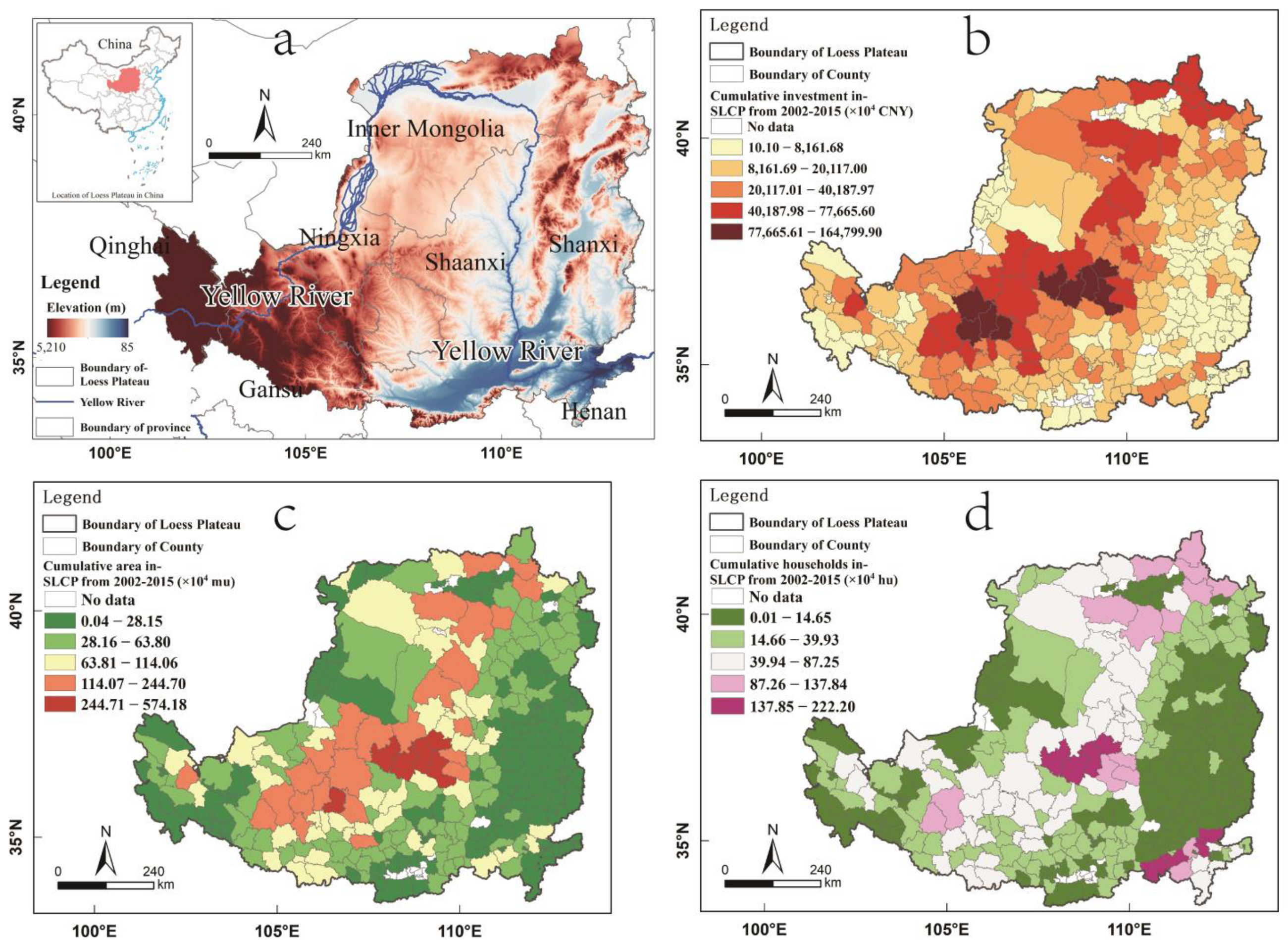
2.1. Study Area

LP is located in the middle and upper reaches of the Yellow River Basin in China (107°28′~111°15′ E 35°21′~39°34′ N), spanning seven provinces and regions in Shanxi, Ningxia, Shaanxi, Gansu, Inner Mongolia, Qinghai, and Henan, with a total area of about 6.49 × 10⁵ km², accounting for 6.7% of China’s land area (Figure 1a). LP terrain slopes from northwest to southeast, with elevation differences exceeding 3000 m. The climate is temperate continental monsoon climate with cold winters and warm humid summers. The average annual temperature ranges from 3.7 to 14.0 °C, and the annual precipitation is 144 to 812 mm, mainly between June and September [27]. The LP is one of the most severe soil erosion and fragile ecosystems in the world due to frequent heavy rainfall, steep topography, low vegetation cover and loose soils [28]. At the same time, the over-exploitation and unreasonable utilization of the resources on the LP have aggravated the soil erosion and led to the serious degradation of land and ecosystem [29,30]. At the end of 1990s, the LP took the lead in implementing the SLCP as a pilot. Through afforestation and other measures, the vegetation coverage was effectively increased, the serious problem of soil erosion was alleviated, and the ecosystems have been greatly restored and improved [31]. By 2015, a total of 154 million mu of cultivated land had been converted to forests on the LP (Figure 1c), with a cumulative financial investment of CNY 61 billion (Figure 1b) and a cumulative participation of 0.9 billion households (Figure 1d).

2.2. Methodology

Figure 2 shows the research framework of this study for the evaluation of EEoSLCP and its spatial and temporal variation. Firstly, based on the definition of the EEoSLCP, the input-output indexes for evaluating the EEoSLCP were determined. Secondly, based on multi-type data such as land use, vegetation NDVI and soil type, various eco-effects of SLCP were obtained with the support of GIS and calculated by models such as pixel dichotomy and RUSLE. Finally, based on the input-output data of SLCP, the DEA-BCC model is applied to measure EEoSLCP, and based on this, the KDE and ESDA models are applied to analyze the spatial and temporal changes of EEoSLCP comprehensively, respectively.

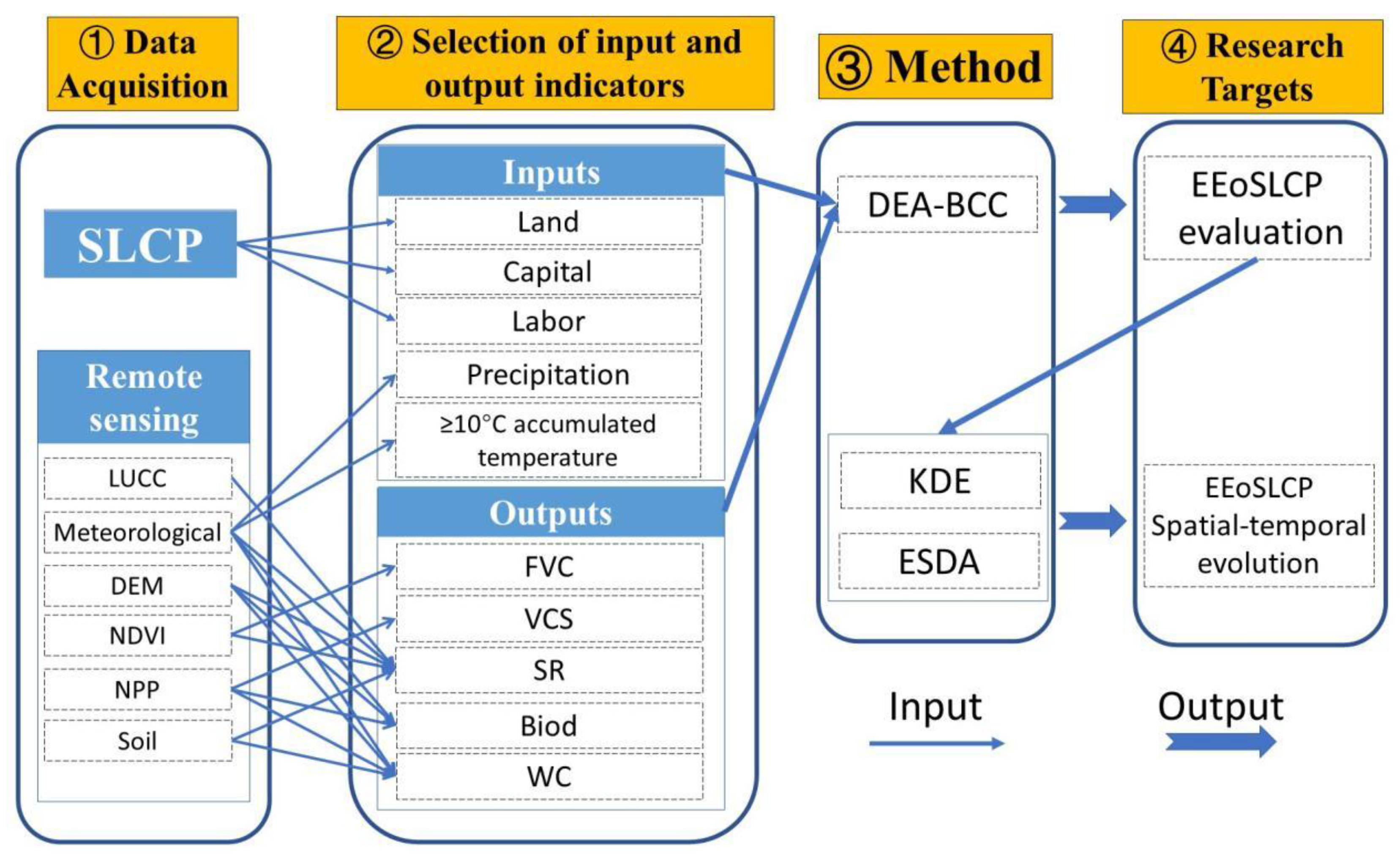
2.2.1. Construction of EEoSLCP Evaluation Index System

Based on the definition of eco-efficiency and the characteristics of the SLCP in practice, we define EEoSLCP as: restoring degraded ecosystems with less resource input in SLCP implementation, producing more ecosystem services to meet human needs, and making the ecosystem environment better. Based on this, we constructed the EEoSLCP evaluation index system in terms of both inputs and outputs (

Table 1. Input and output indicators of EEoSLCP.

Indicator	Variable	Variable Description	Unite
Input	Land	Cumulative area of SLCP implementation	mu *
	Capital	SLCP cumulative financial investment	CNY *
	Labor	Cumulative number of SLCP participating households	hu *
	≥10 °C accumulated temperature	Average annual ≥10 °C accumulated temperature	°C
	Precipitation	Average annual precipitation	mm
Output	VFC	Cumulative increase in average VFC compared to 2002	%
	SR	Cumulative increase in average SR compared to 2002	t·hm−2·yr−1
	VCS	Cumulative increase in average VCS compared to 2002	gC·m−2·yr−1
	WC	Cumulative increase in average WC compared to 2002	dimensionless, value range 0–1
	Biod	Cumulative increase in average Biod compared to 2002	dimensionless, value range 0–1

*: mu is the Chinese unit of land measurement; 1 mu is equal to 1/15 hm². The CNY is the base unit of a number of former and present-day currencies in Chinese; 1 USD equals CNY 6.70 as of 13 January 2023 (https://www.federalreserve.gov/releases/h10/current/ (accessed on 13 January 2023)). According to the 7th national census bulletin released by the China Statistics Bureau, 1 hu equals approximately 2.62 people. (http://www.stats.gov.cn/tjsj/tjgb/rkpcgb/qgrkpcgb/202106/t20210628_1818821.html (accessed on 13 January 2023)).

). For the inputs, we chose three indicators closely related to SLCP: capital, land, and labor. At the same time, considering SLCP as a reforestation program, its ecological benefits are not only influenced by the input of the program itself but also by the natural conditions [32,33]. Numerous studies have shown that temperature and precipitation are the main natural factors that determine the effectiveness of SLCP on the LP [34,35]. For this reason, we also selected precipitation and temperature as input indicators. In terms of output, we selected five indicators that best reflect the ecological changes on the LP, namely: vegetation fraction cover (VFC), vegetation carbon sequestration (VCS), soil retention (SR), biodiversity (Biod) and water conservation (WC). The specific process and reasons for the selection of EEoSLCP evaluation indicators are explained in detail in our published paper [33]. The references involved in the selection of evaluation indicators are: [10,13,14,15,16,18,32,36,37,38,39,40,41].

2.2.2. Eco-Effects Calculation of SLCP

We calculated and analyzed the spatial and temporal changes of eco-effects such as VFC and VCS on the LP from 2002 to 2018 after the implementation of SLCP by collecting various remote sensing data obtained from land use, vegetation NDVI, DEM, and meteorology, using GIS technology. Please refer to the supplementary materials [33] of our published paper [33] for the specific formulae and results of the five eco-effects of VFC, VCS, SR, WC, and Biod in the Loess Plateau from 2002 to 2018. The references for the calculation of the five eco-effects of the Loess Plateau are: [42,43,44,45,46,47,48,49,50,51,52,53,54,55,56,57,58,59].

2.2.3. Ecological Efficiency Calculation of SLCP

(1)

DEA model

The core idea of the DEA model is to keep the input or output values of the decision units constant, project the decision units onto the effective frontier surface with the help of the linear programming principle, and then compare the deviation of the decision units from the effective frontier surface to evaluate their relative effectiveness. Using this method, we can not only derive the efficiency between input and output variables, but also the direction from which we need to improve each input variable in order to enhance the overall efficiency. DEA models are divided into CCR models with constant returns to scale and BCC models with variable returns to scale [60,61,62]. Considering that the ecological benefits obtained from the implementation of SLCP are characterized by variable payoffs to scale, we will complete the measurement of EEoSLCP for the LP using the DEA-BCC model. The specific model is as follows.

$$\min {\theta }_z-\epsilon ({\displaystyle \sum _{i=1}^m{s}_i{}^{-}}+{\displaystyle \sum _{r=1}^s{s}_r{}^{+}})$$

(1)

$$s.t.{\displaystyle \sum _{j=1}^n{\lambda }_j{x}_{ij}+s_i{}^{-}={\theta }_{z}i{x}_{rz},i=1,2,\cdots ,m}$$

(2)

$${\displaystyle \sum _{j=1}^n{\lambda }_j{y}_{rj}-s_i{}^{+}=y_{rz},r=1,2,\cdots ,s}$$

(3)

$${\displaystyle \sum _{j=1}^n{\lambda }_j=1}$$

(4)

$${\theta }_0,{\lambda }_j,s_i{}^{-},s_i{}^{+}\ge 0$$

(5)

where θ_z is the EEoSLCP in the LP under VRS, where n =314 is the number of counties in the LP, j represents the jth county, which can also be called the jth DMU. m and s, respectively, represent the number of input–output indicators of SLCP, x_ij represents the input of the i factor in the jth county, y_rj represents the r output in the jth county, and λ_j is the weight coefficient of the input index of a certain factor in the jth county. When the sum of S_i^- and S_r⁺ is 0, all input and output are in a relaxed state, θ_z = 1, and the EEoSLCP is in complete efficiency. When the sum of S_i^- and S_r⁺ is not 0, θ_z < 1, the EEoSLCP is in incomplete efficiency, and the complete efficiency can be achieved again by adjusting the level of input or output.

(2)

Kernel Density Estimation (KDE)

KDE is an important method to study spatial disequilibrium distribution, which is surface interpolation through discrete sampling points [63]. It is a nonparametric estimation method in which the position, shape, and extensibility of random variables are described by continuous smooth density curves instead of histograms. The kernel function mainly includes linear kernel function, polynomial kernel function, Gaussian kernel function, etc. In this paper, we choose the more commonly used Gaussian kernel function. Assuming that the density function of the random variable x is f(x), the kernel density is estimated as [64]:

$$f(x)=\frac{1}{Nh}{\displaystyle \sum _{i=1}^{N}K}\left(\frac{X_i-\overline{x}}{h}\right)$$

(6)

$$K(x)=\frac{1}{\sqrt{2\mathsf{\Pi }}}\exp \left(-\frac{x^2}{2}\right)$$

(7)

where K(·) is the kernel function; N is the number of observations; X_i is the independent observation with the same distribution; $\overline{\mathit{x}}$ is the mean; h is the bandwidth, which determines the smoothness and accuracy of the estimated density curve. The larger the bandwidth, the smaller the variance of the kernel estimation and the smoother the curve.

(3)

Exploratory Spatial Data Analysis (ESDA)

ESDA is a collection of a series of spatial data analysis methods and techniques, which takes spatial association measure as the core, and distinguishes spatial agglomeration and spatial differentiation by describing and visualizing the spatial distribution pattern of things or phenomena, so as to reveal the spatial dependence among objects. ESDA consists of global spatial autocorrelation (GSA) and local spatial autocorrelation (LSA) [65].

GSA is mainly used to judge whether a phenomenon has clustering characteristics in space, which is generally measured by Moran’s I index, and its calculation formula is [66]:

$$I=\frac{{\displaystyle \sum _{i=1}^n{\displaystyle \sum _{j=1}^n{W}_{ij}}}\left(Y_i-\overline{Y}\right)\left(Y_j-\overline{Y}\right)}{S^2{\displaystyle \sum _{i=1}^n{\displaystyle \sum _{j=1}^n{W}_{ij}}}}$$

(8)

Among them, $S^2=\frac{1}{n}{\displaystyle \sum _{i=1}^n{\left(Y_i-\overline{Y}\right)}^2}$, $\overline{Y}=\frac{1}{n}{\displaystyle \sum _{i=1}^n{Y}_i}$, Y_i is the EEoSLCP for county i, n is the number of samples, and the sample number in this study refers to the 314 counties in the LP; Y is the average of EEoSLCP in all counties; W_ij is the spatial weight matrix, which represents the influence factors between counties i and j and constitutes a complete set of spatial relationships. Moran’s I value range is [−1,1]. When I is greater than 0, it indicates that there is a positive spatial correlation between regions and, the closer it is to 1, the more similar observed values (high or low values) tend to gather in space. When I is less than 0, it shows that there is a spatial negative correlation between regions and, the closer it is to −1, the more scattered the similar observations tend to be in space. When I is equal to 0, it shows that there is no spatial correlation between regions and the observed values tend to be randomly distributed.

GSA mainly explains the average correlation degree of a phenomenon in space, but cannot clearly reflect which areas in the study area have agglomeration. LSA is an index to measure the spatial correlation of the research object from the local perspective, which measures the similarity between the regional observations in this area and the observations in neighboring areas, and can be used to identify the agglomeration and discrete characteristics of the local spatial pattern [65]. It is usually measured by local Moran’s I index and its calculation formula is [66]:

$$I_i=Z_i{\displaystyle \sum _{j=1}^n{W}_{ij}}{Z}_j$$

(9)

where $Z_i=Y_i-\overline{Y}$, $Z_j=Y_j-\overline{Y}$, Y_i, Y_j denote the observed values of the ith and jth region, which is the EEoSLCP in this study, n is the number of samples, the sample number in this study refers to the 314 counties in the LP, and W_ij is the spatial weight matrix. The local Moran’s I index measures the degree of correlation between the ith region and other surrounding areas. If I_i > 0, it means that the local area neighboring units are spatially clustered with similar values; if I_i < 0, it means that the local area neighboring units are not spatially clustered with similar values; if I_i = 0 means that the local area neighboring units are spatially randomly distributed. Specifically, LSA analysis can be divided into the following four types: high–high cluster (H-H), high–low outlier (H-L), low–high outlier (L-H), and low–low cluster (L-L).

2.2.4. Data Sources

The data of this study include remote sensing data, land use data, meteorological data, soil data, and other multi-source data sets. All the raster data below are processed with a resolution of 500 m and the coordinate system is Krasovsky_1940_Albers. The data sources of this study are as follows:

The land use map data of 2000, 2005, 2010, and 2018 were downloaded from the Data Center for Resources and Environmental Sciences, Chinese Academy of Sciences (RESDC) (https://www.resdc.cn/ (accessed on 5 May 2021)), including cultivated land, forests, grassland, water area, construction land, and unused land. The spatial resolution of the data was 30 m. The land use data of each period were verified and modified by field survey, and the combined precision of the data in 2000 was 92.9% [67], in 2005 was 95% [68], in 2010 was 94.3% [69], and in 2018 was 95.53% [70].

In the meteorological data, precipitation and temperature from 2002 to 2018 was obtained from the Chinese National Meteorological Science Data Service Center (http://data.cma.cn/ (accessed on 6 September 2020)). Moreover, ≥10°C accumulated temperature from 2002 to 2015 was obtained from the National Ecosystem Science Data Center (http://www.nesdc.org.cn (accessed on 5 May 2021)). Furthermore, via ArcGIS software using the Kriging interpolation method, we obtained the meteorological raster dataset.

The digital elevation model (DEM) data used in the study is ASTER GDEM V2, with a spatial resolution of 30 m, downloaded from Japan Space Systems.

The NDVI from 2002 to 2018 was derived from the MOD13A1 product synthesized by the maximum value composite (MVC) method 16d and downloaded from the NASA MODIS website with a spatial resolution of 500 m (https://ladsweb.modaps.eosdis.nasa.gov/search (accessed on 5 May 2021)).

The net primary productivity (NPP) from 2002 to 2018 was derived from the MOD17A3HGF database of the Terra Net Primary Production and downloaded from the NASA MODIS website with a spatial resolution of 500 m (https://ladsweb.modaps.eosdis.nasa.gov/search (accessed on 5 May 2021)).

Soil attribute data were obtained from the China soil map based harmonized world soil database (HWSD) (v1.1) (2009) shared by the National Tibetan Plateau/Third Pole Environment Data Center (https://data.tpdc.ac.cn/ (accessed on 5 May 2021)), which was provided by the Second National Land Survey data from the Nanjing Institute of Soil Research, Chinese Academy of Sciences.

The data of SLCP financial investment and project implementation area of 314 counties in the LP from 2002 to 2015 were obtained from the Central South Survey and Planning Institute under the National Forestry and Grassland Administration of China (http://www.forestry.gov.cn/sites/zny/zny/ (accessed on 5 May 2021)). The number of farm households participating in the SLCP is based on provincial data published in the China Forestry Statistical Yearbook (2003–2016) and obtained by proportional conversion of financial investment data in each county.

Administrative boundaries of the cities are obtained from the national 1:1,000,000 database of China Geographic Information Monitoring Platform (https://www.webmap.cn (accessed on 5 May 2021)).

3. Results

3.1. Eco-Effects of SLCP

From 2002 to 2018, after implementing SLCP on the LP, the ecological afforestation effect was remarkable, the ecological environment was significantly improved, and the growth of each eco-effect was remarkable. Firstly, from the temporal changes of various eco-effects (Figure 3a–e), the average VFC increased from 50.12% to 64.15%, with a growth rate of 27.99%; the average VCS increased from 883.54 gC·m⁻²·yr⁻¹ to 1296.35 gC·m⁻²·yr⁻¹, with a growth rate of 46.72%; the average SR increased from 221.11 t·hm⁻²·yr⁻¹ to 228.41 t·hm⁻²·yr⁻¹, with a growth rate of 3.3%; the average WC increased from 0.1458 to 0.1643, with a growth rate of 12.73%; and the average Biod increased from 0.1549 to 0.1815, with a growth rate of 17.12%. Secondly, from the spatial change trend of the eco-effects of the LP from 2002 to 2018 (Figure 3f–j), the eco-effects of the southwest, central, and northeast of the LP have been significantly improved.

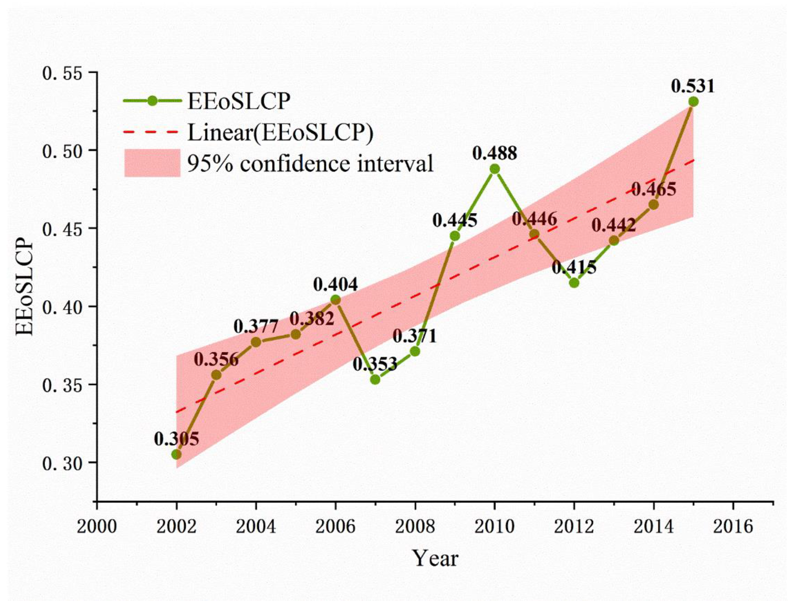
3.2. Temporal Changes and Evolution of EEoSLCP

The EEoSLCP of the LP and its 314 counties from 2002 to 2015 was measured using the DEA-BCC model selected by MaxDEA software. Figure 4 shows the average score of EEoSLCP for LP from 2002 to 2015. Firstly, it was found that the average EEoSLCP score for the LP from 2002 to 2015 was low, with an overall average score of only 0.413. Secondly, the EEoSLCP presented an overall growth trend from 0.305 in 2002 to 0.531 in 2015, indicating that EEoSLCP has been effectively improved over time. Finally, based on the trend of EEoSLCP changes on the LP during 2002–2015, the temporal changes of EEoSLCP can be divided into three stages in conjunction with the implementation of SLCP during the study period: the first stage was from 2002 to 2006, in which the EEoSLCP increased year by year; the second stage was from 2006 to 2010, in which the EEoSLCP decreased first (2006–2007) and then increased (2007–2010); the third stage was from 2010 to 2015, in which the EEoSLCP also decreased first (2010–2012) and then increased (2012–2015).

Figure 5 is obtained after kernel density calculation by Matlab R2018a (Matlab software from MathWorks, Inc., Natick, MA, USA).

(1)

In terms of the distribution position, the overall EEoSLCP on the LP shows a “rightward” distribution from left to right, with peaks from high to low, and the curve tends to flatten out with increasing years, with a small shift to the right, indicating that the number of counties with high eco-efficiency is increasing and the number of counties with relatively low efficiency is decreasing, implying that the eco-efficiency of each county is steadily improving over time.

(2)

From the distribution pattern, the overall distribution curve of EEoSLCP on the LP shows the evolution pattern of “two peaks standing side by side” composed of “one main peak plus one side peak”. It shows that the EEoSLCP in each county of the LP is always in the pattern of polarization during the study period and the eco-efficiency of some counties is concentrated at a higher level, while that of other counties is concentrated at a lower level. From 2002 to 2015, the evolutionary dynamics of the main peak height showed an overall decrease over time and an increase in the width of the main peak, indicating that the absolute gap in efficiency tends to widen in counties clustered at a lower level of EEoSLCP. The evolution of the height of the lateral peaks shows an overall increase over time and a gradual decrease in width, indicating that the absolute difference in efficiency tends to decrease in counties clustered at a higher level of EEoSLCP.

(3)

In terms of polarization characteristics, the EEoSLCP in the LP from 2002 to 2015 shows the phenomenon of “bimodality” and polarization, with relatively large distances between the side peaks and the main peaks, and obvious differences in eco-efficiency between counties on the LP, gradually forming a “bimodal” evolution pattern of “low–low agglomeration and high–high agglomeration”, which is similar to “club convergence”.

3.3. Spatial Distribution of EEoSLCP

Based on the EEoSLCP of each county in the LP from 2002 to 2015, the EEoSLCP of each county was classified into four states of low efficiency (0, 0.25], medium–low efficiency (0.25, 0.5], medium–high efficiency (0.5, 0.75], and high efficiency (0.75, 1] with reference to previous studies [33]. From Figure 6, it can be seen that the EEoSLCP of most counties in the LP is low-efficiency during the study period, mainly distributed in the central, northern, and western regions in a contiguous manner. There are fewer medium–low efficiency counties in the study period, which are mainly distributed in the middle of high-efficiency and medium-high efficiency counties in the southern and eastern regions, distributed in a northeast–southwest strip. Fewer counties have medium–low efficiency status, and they are mainly concentrated in the middle of high efficiency and medium–high efficiency counties in the southern and eastern regions, distributed in a northeast–southwest strip. The spatial distribution areas of high efficiency and medium–high efficiency counties are roughly the same, mainly distributed in the eastern, southern, and western regions. Overall, although the EEoSLCP has obvious spatial heterogeneity among counties in the LP, it presents a distribution trend that gradually decreases from southeast to northwest and from south to north.

From the number of counties divided into efficiency status intervals (Appendix A, Figure A1), the number of counties with low EEoSLCP showed a fluctuating downward trend, from 161 in 2002 to 76 in 2015, mainly concentrated in the southeastern part of the LP, and the range of counties with low efficiency shrank from southeast to northwest year by year. The number of counties with high efficiency and medium efficiency showed a fluctuating upward trend, from 60 and 35 in 2002 to 114 and 69 in 2015, respectively, mainly located in the central and eastern regions of the LP. The number of medium–low efficiency counties shows a stable and unchanging trend, basically stable at about 50.

3.4. Spatial Correlation of EEoSLCP

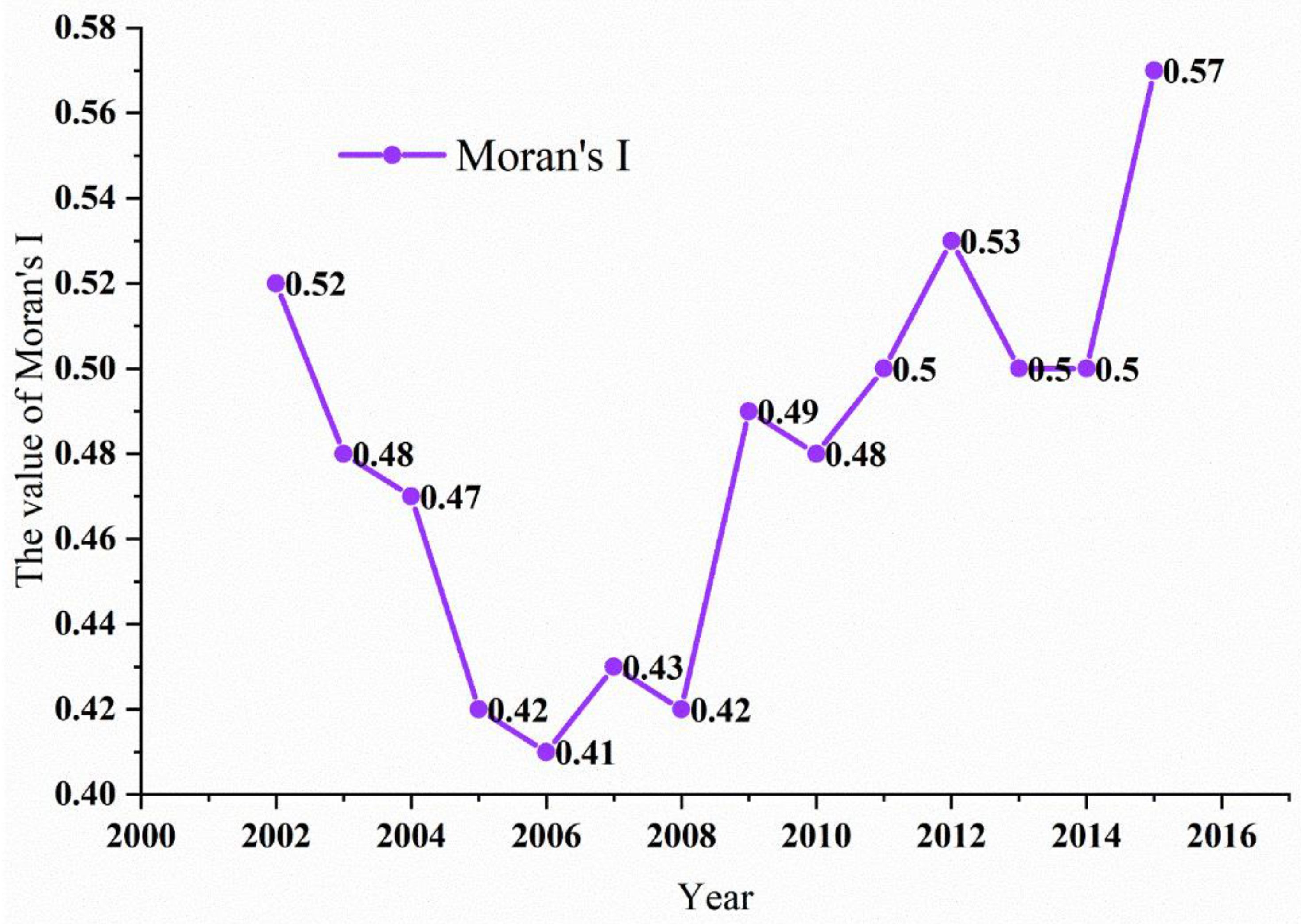
3.4.1. GSA Analysis

Based on the ESDA model, ArcGIS software was used to calculate the global Moran’s I index of EEoSLCP in the LP from 2002 to 2015. From Figure 7, it can be concluded that the global Moran’s I index was positive, ranging from 0.41 to 0.57, and all of them passed the significance test at the 1% level (Appendix A,

Table A1. Global Moran’s I value and its test results of EEoSLCP in the LP from 2002 to 2015.

Year	Moran’s I	Z	p
2002	0.518 ***	14.532	0.000
2003	0.481 ***	13.490	0.000
2004	0.470 ***	13.192	0.000
2005	0.424 ***	11.911	0.000
2006	0.414 ***	11.637	0.000
2007	0.432 ***	12.123	0.000
2008	0.420 ***	11.807	0.000
2009	0.494 ***	13.857	0.000
2010	0.484 ***	13.588	0.000
2011	0.504 ***	14.137	0.000
2012	0.534 ***	14.964	0.000
2013	0.496 ***	13.924	0.000
2014	0.499 ***	13.985	0.000
2015	0.565 ***	15.852	0.000

Note: *** denote statistical significance at 1%, 5%, and 10%, respectively.

), indicating that the EEoSLCP in each county of the LP showed positive spatial autocorrelation. Its spatial connection characteristics are as follows: the counties with higher eco-efficiency tend to be adjacent to the counties with higher eco-efficiency, while the counties with lower eco-efficiency tend to be adjacent to the counties with lower eco-efficiency; that is, the adjacent counties mostly show the spatial agglomeration characteristics of “high–high” or “low–low”, but seldom show the spatial agglomeration characteristics of “high–low” or “low–high”. The spatially positive autocorrelations of the EEoSLCP in each county of the LP show a relatively stable trend. The positive spatial correlation of the EEoSLCP decreased from 2002 to 2006, increased from 2006 to 2007, decreased again from 2007 to 2008, first increased, then decreased and then increased from 2008 to 2012, then decreased from 2012 to 2013, and finally increased from 2013 to 2015. Its spatial pattern is more obviously clustered in all years except for two years in 2006 and 2008 when it showed weak clustering distribution. The global Moran’s I value was the lowest in 2006 at 0.41 and the highest in 2015 at 0.57. This indicates that the spatial agglomeration state of the EEoSLCP of the Loess is relatively stable but also has some fluctuations. Specifically, the relative positions of the spatial pattern of the EEoSLCP in neighboring counties are basically constant, but their relative differences are variable and show certain strong and weak variations.

3.4.2. LSA Analysis

The global Moran’s I index can prove that there is a positive spatial correlation in the EEoSLCP on the LP, but it cannot reflect its local spatial characteristics. Therefore, the local Moran’s I index is needed to identify the local spatial characteristics of the EEoSLCP in each county of the LP. According to Figure 8 and Appendix A, Figure A2, the specific local spatial pattern and distribution quantity can be classified into the following four categories:

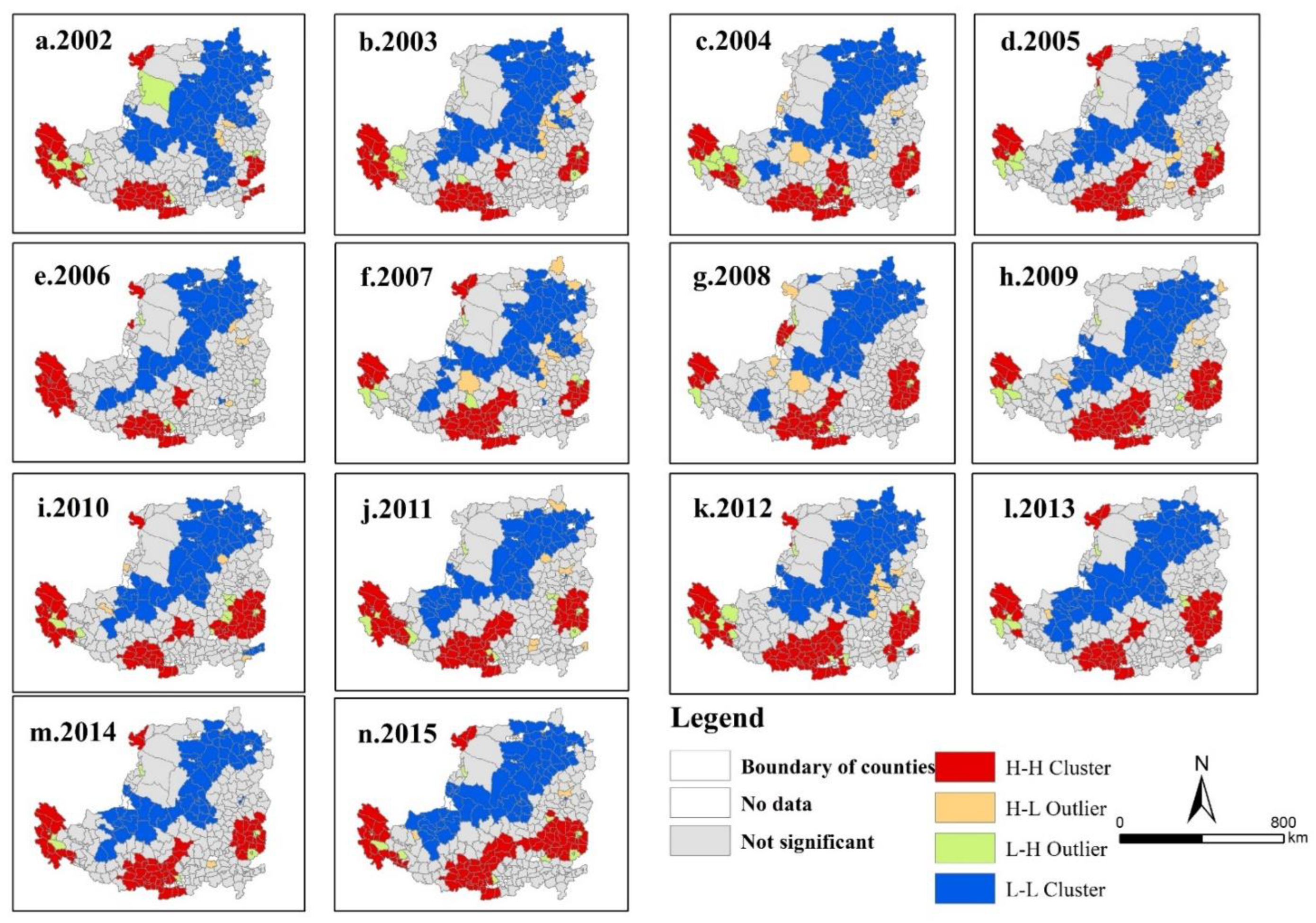
(1)

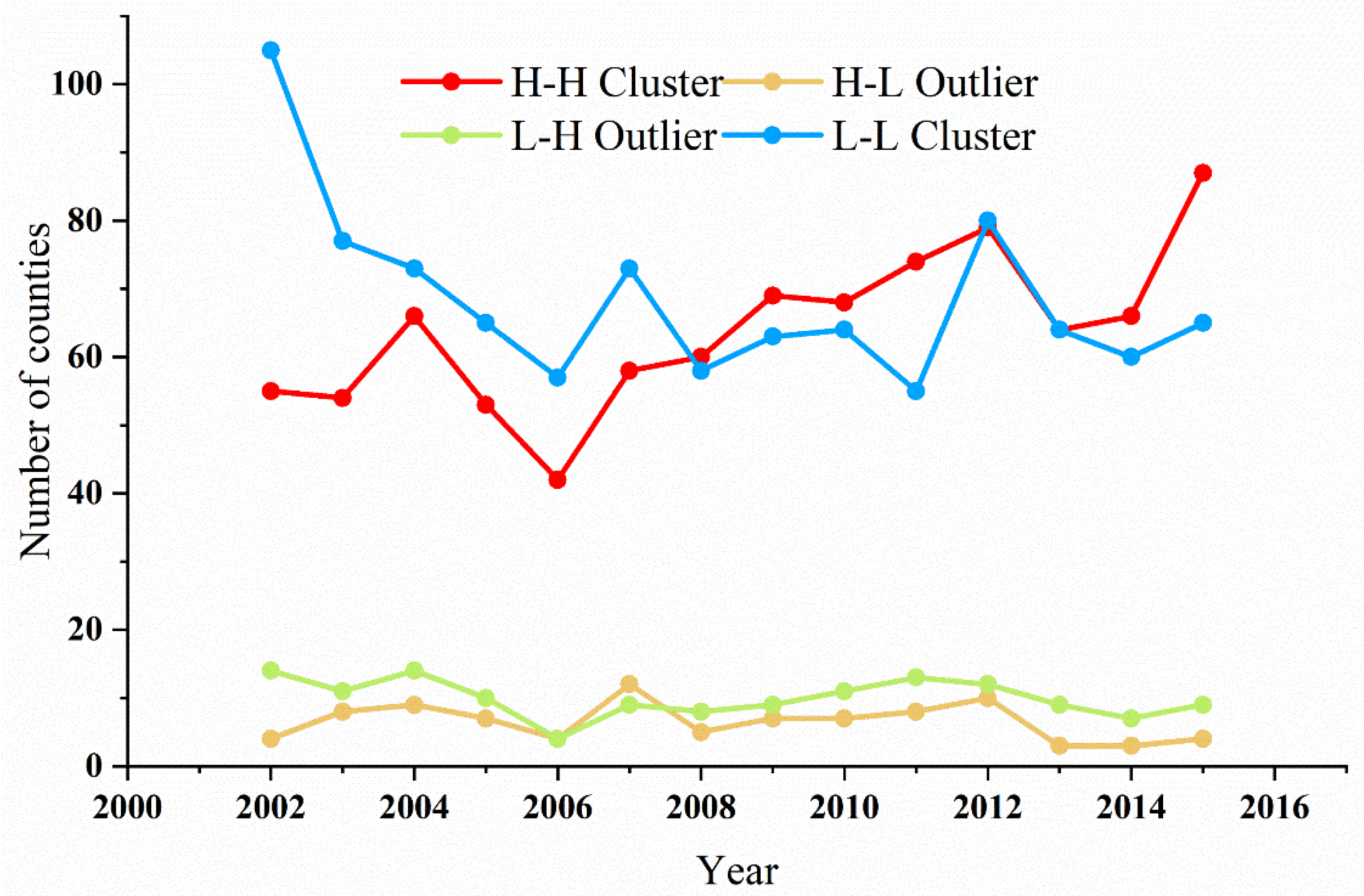
H-H clustering, which indicates that, if a county has high EEoSLCP, then its neighboring counties also have high efficiency, mainly concentrated in the western, southern, and eastern regions, which is a high level of the spatial equilibrium associated agglomeration state of “high in the center and high around”. The number of H-H in 2002 to 2015 showed an overall fluctuating upward trend in time and, in space, it showed that the range of the H-H clusters in the west remained basically unchanged, while the H-H clusters in the south expanded and spread to the north and northeast, and the H-H clusters in the southeast corner region expanded and spread to the south and to the west.

(2)

L-H outlier, which indicates that, although the EEoSLCP of a county is low, the efficiency of its neighboring counties is high, sporadically distributed in the western and eastern parts of the LP, showing a spatially unbalanced correlated agglomeration of “low in the center and high in the surroundings”. This trend is spatially distributed in the western and eastern regions.

(3)

L-L clustering, which indicates that not only is the EEoSLCP of a county low but also the efficiency of its neighboring counties is low, mainly concentrated in the central, northern, and northeastern areas of the LP, with an overall “southwest–northeast” distribution, showing a low level of spatial equilibrium associated with the clustering state of “low in the center and low around”. The number of L-L in 2002–2015 showed a fluctuating decline in time and a gradual decrease in space from the southeast to the northwest, but the L-L cluster in the southwest showed a continued spreading and expanding trend to the southwest.

(4)

H-L outlier, which indicates that, although a county has high EEoSLCP, its neighboring counties have low efficiency, mainly scattered in the central and eastern parts of the LP, showing a spatially unbalanced correlated clustering state of “high in the center and low around”. The number of such counties is small, and the temporal change increases then decreases, and this trend is spatially distributed in the central region.

Overall, the number of local spatial characteristics of the EEoSLCP in the LP during the study period was L-L > H-H > L-H > H-L. Further analysis of the local spatial pattern of EEoSLCP in each county shows that there is a strong spatial neighboring companion effect of EEoSLCP among the counties in the LP. Specifically, in the LP, when the EEoSLCP around a county is at a high (low) level, its own efficiency tends to reach a high (low) level.

4. Discussion

4.1. Analysis of Temporal Changes in EEoSLCP

Our research shows that the ecological environment of the LP has been greatly improved after the implementation of SLCP. Good ecological benefits have been achieved in VFC, VCS, SR, and other aspects, which is consistent with the research results of previous scholars [9,10,11,12,13,14,15,16,17,18]. However, from the perspective of efficiency, we found that the average EEoSLCP score for the LP from 2002 to 2015 was low, with an overall average score of only 0.413. The reason for this is that SLCP is a top-down, government-led ERP [7], and the implementation of the program involves a wide range of tasks and high construction requirements, although the construction of the project has achieved good eco-effects. However, the lack of scientific proof, empirical guidance, and a scientific supervision system for project implementation, coupled with the generally low compensation standard for households, makes it difficult to create a sustainable incentive for the households to participate in the program, which eventually leads to low EEoSLCP [71,72]. However, from the temporal changes of EEoSLCP, it can be obtained that, from 2002 to 2015, the overall EEoSLCP on LP has been growing and the growth rate has gradually accelerated. The reason is that 2002–2006 is still the initial stage of the SLCP implementation, although a lot of investment, land, and households have been input; however, because of the irrational planting structure of economic forests (the planting proportion of economic forests is far greater than ecological forests) [73], the low quality of afforestation [74,75] and the low subsidy standard [71,74], etc. As a result, eco-efficiency is always on the low side at this stage and the growth rate is slow. The period 2007–2010 was the optimization and adjustment phase of SLCP and the problems that existed before were greatly solved by learning the lessons from the implementation of SLCP in the previous phase. More importantly, the State Council decided to increase cash subsidies for participating SLCP households and to prolong the subsidy period for those who are enjoying the subsidy expiration [76,77], and also decided to give households a certain degree of autonomy in SLCP participation [78], which greatly motivated households to participate in the SLCP, improved the afforestation quality of SLCP implementation, and finally achieved greater ecological benefits [79]. Therefore, EEoSLCP was able to ramp up rapidly during this stage. The period 2011–2015 was the consolidation and improvement stage of the SLCP, and the EEoSLCP decreased and then increased in this stage. The reason is that, since 2011, the main task of SLCP has been adjusted to consolidate the ecological achievements made in the previous period but, in practice, due to the lack of subsidy distribution, lack of supervision, and backward management techniques, some of the trees planted in the previous period have died and some districts and counties have even experienced the phenomenon of deforestation and replanting [74,80,81]. However, the central government still provides financial subsidies according to the completed area of SLCP in each county, resulting in a decrease in the input–output ratio and a decline in eco-efficiency from 2011 to 2012. After 2013, local governments began to subsidize households participating in SLCP with their own funds so as to further improve the results of SLCP and strengthened the management of the results of SLCP implementation. Meanwhile, the implementation of a new round of SLCP after 2014 not only led to the expansion of afforestation area but also further improved and consolidated the achievements of the previous SLCP, which eventually led to a renewed increase in EEoSLCP between 2013 and 2015.

4.2. Analysis of the Spatial Pattern of EEoSLCP

Low–low agglomeration area in the northern part of LP. A large part of this area is located in sandy land and desert areas, which belong to arid and semi-arid regions. The growth and survival of vegetation are strictly limited by the supply of water resources [82,83]. Although the SLCP has input a certain amount of area (Figure 1c), investment (Figure 1b), and households (Figure 1d) in the region, the precipitation (Appendix A, Figure A3a) and ≥10 °C accumulated temperature (Appendix A, Figure A3b) conducive to the growth of vegetation are very limited, coupled with the unreasonable selection of tree species, leading to a low afforestation survival rate, and it is difficult to achieve the expected eco-effects of afforestation in sandy and desert areas [84]. In addition, the presence of sparse trees can concentrate airflow between trees, thereby increasing wind speed and erosion forces, and increasing soil drying and erosion when trees are unable to block strong winds, instead accelerating the rate of land degradation within sandy desert areas and further exacerbating the degree of desertification within the region [85,86]. As mentioned above, due to the limitation of precipitation and accumulated temperature, it is difficult to effectively convert the input of SLCP into eco-effects in the northern part of LP, which leads to the low EEoSLCP in this region.

Low–low agglomerations in the central and western parts of the LP. Most of this area is located in the hill and gully region of the LP in Shaanxi and Gansu, where soil and water loss is the most serious, so the counties in this area have always been the key areas for the implementation of SLCP. From 2002 to 2015 the region was the most invested in the LP Retirement Forestry Project. The counties belonging to this region were the areas that received the most input from the SLCP from 2002 to 2015 (Figure 1b–d). In terms of effect, the VFC, VCS, SR, WC, and Biod in the area have been significantly improved (Figure 3f–j), indicating that the implementation of SLCP in the area has achieved significant eco-effects. However, in terms of efficiency, the EEoSLCP in the above areas has been low. In order to find the reasons, we conducted statistics on the average input redundancy and average output deficiency of the SLCP in 314 counties of the LP. The reason for this is that the above-mentioned areas have higher redundancy in terms of area (Appendix A, Figure A3c), investment (Appendix A, Figure A3d), and households (Appendix A, Figure A3e) inputs for the SLCP, and at the same time higher deficiency in terms of eco-effects outputs such as VFC, VCS, and SR (Appendix A, Figure A4a–e). Therefore, although the aforementioned areas have achieved good eco-effects with a large amount of investment, land, and labor resources invested, excessive input redundancy and deficiencyoutput have led to low EEoSLCP in the area.

Medium–high and high-efficiency agglomerations in the eastern and southern parts of the LP. The region is in a semi-humid area and has precipitation (Appendix A, Figure A3a) and ≥10 °C temperature accumulation (Appendix A, Figure A3b) conditions that are more suitable for vegetation growth than other areas of the LP. Secondly, the above-mentioned areas have low redundancy in the investment of area (Appendix A, Figure A3c), investment (Appendix A, Figure A3d), and households (Appendix A, Figure A3e) for SLCP and, at the same time, the deficiency in eco-effects such as VFC, VCS, and SR is also low (Appendix A, Figure A4a–e). As a result, the conversion rate between input and eco-effects output of SLCP in the above areas is higher, so the EEoSLCP is also higher.

4.3. Analysis of the Spatial Correlation of EEoSLCP

ESDA of the EEoSLCP showed that there was a significant positive spatial correlation between the EEoSLCP among counties in the LP. This not only proves once again that there is an obvious spatial clustering characteristic of the EEoSLCP in each county (Figure 6) but also further indicates that there is a strong spatial dependence of the EEoSLCP in some counties. However, according to the change of global Moran’s I index (Figure 7), the global Moran’s I index showed a downward trend from 2002 to 2006, indicating that the spatial dependence of EEoSLCP in each county of the LP showed a weakening trend. This may be because, in the initial stage of the implementation of SLCP, various places are still in the exploratory stage and, with the implementation of SLCP moving forward, the gap between the implementation technology and management level of the program gradually appears [87,88], which leads to the increasing relative difference in the spatial EEoSLCP implementation in each county, and the spatial dependence is gradually weakened. The global Moran’s I index showed an increasing trend from 2006 to 2015, indicating the increasing spatial dependence of the EEoSLCP in each county of the LP. This may be due to the fact that all localities have learned from the previous program implementation experience at this stage and, by actively learning from the surrounding counties with high eco-efficiency [78,89], the level of program implementation technology and management has been improved, and the eco-efficiency has been improved. Thus, the relative spatial difference of eco-efficiency in each county continues to narrow and the spatial dependence is gradually enhanced.

Further, from the local autocorrelation results of the EEoSLCP in each county on the LP, it can be seen that the neighboring counties mostly show “H-H” or “L-L” clustering, and the number of counties with “H-H” clustering is expanding, while the number of counties with “L-L” clustering is decreasing (Figure 8). The range of the H-H cluster area has been expanding along the H-H cluster area at the early stage of SLCP implementation (Figure 8), probably because the southern and southeastern counties of the LP have attracted neighboring counties to learn afforestation and management experience through the demonstration effect [78,89], which has led to the increasing conversion rate of the inputs to the eco-effects output of SLCP, thus promoting the improvement of the EEoSLCP. The scope of the L-L cluster area gradually shrinks along the L-L cluster area at the beginning of SLCP implementation, which may be related to the warning effect brought by the low efficiency counties. Officials in some counties have been punished for poor implementation of SLCP and corruption [73]. The resulting warning effect will motivate officials in L-L catchment counties to take the initiative to learn from the experience of neighboring counties with high eco-efficiency, improve engineering and management levels, and increase the conversion rate of SLCP inputs eco-efficiency, which in turn has led to improved eco-efficiency.

4.4. Limitation and Future Directions

Nonetheless, this study has several limitations. First, in terms of the temporal selection of the study, due to the limitation of data acquisition, we only assessed the eco-efficiency of the first round of SLCP implemented in 314 counties in the LP from 2002 to 2015. However, the Chinese government has started to implement a new round of SLCP after 2015, so what is the eco-efficiency of the new round of SLCP implemented from 2015 to the present? How does the eco-efficiency of the two different periods compare? All of the above questions need to be addressed in our future research. Second, in the selection of eco-efficiency output indicators of SLCP, we have selected the core indicators that are commonly used and easily quantified by academia. However, a comprehensive measurement of the EEoSLCP may need to include more eco-efficiency output indicators of SLCP, such as sandstorm prevention, flood mitigation, air purification, etc., which will be the direction of further research on the measurement of EEoSLCP. Third, in the analysis of the drivers of the ecological efficiency of SLCP, this study uses a combination of qualitative and quantitative methods to analyze to some extent the possible reasons that may affect the spatial and temporal evolution of the EEoSLCP, but the SLCP is a complex socioeconomic ecological system project, which requires us to explore the inner mechanism and driving mechanism of the spatial and temporal evolution of the EEoSLCP through the establishment of econometric models in future studies.

5. Conclusions and Policy Implications

5.1. Main Conclusions

“The UN Decade on Ecosystem Restoration 2021–2030” strategy and China’s “carbon peaking and carbon neutrality” strategy marked the beginning of a large-scale ERP. At the same time, the full-scale ecological restoration project also implies a large investment of capital, labor, and other resources. However, the scarcity of resources determines that we have limited resources to invest in ERPs and failure to convert the limited resources into ecological restoration effectiveness in the implementation of ERPs will hinder the realization of the above two strategic goals. To this end, we take the world’s largest ERP, the SLCP, as an example and evaluate its eco-efficiency, with a view to summarizing the lessons learned and then providing reference for improving the resource utilization efficiency in the implementation of ERPs under resource constraints, and ultimately promoting the realization of the above two strategic goals. This study takes LP, the core region of SLCP implementation, as the study area, and uses the DEA-BCC model to measure the EEoSLCP of LP counties based on the SLCP input–output data of 314 counties in LP and, on this basis, the KDE and ESDA methods are used to portray and identify the time-series dynamic evolution pattern and spatial pattern evolution characteristics of EEoSLCP from a two-dimensional perspective in time and space, respectively. The major findings were as follows:

(1)

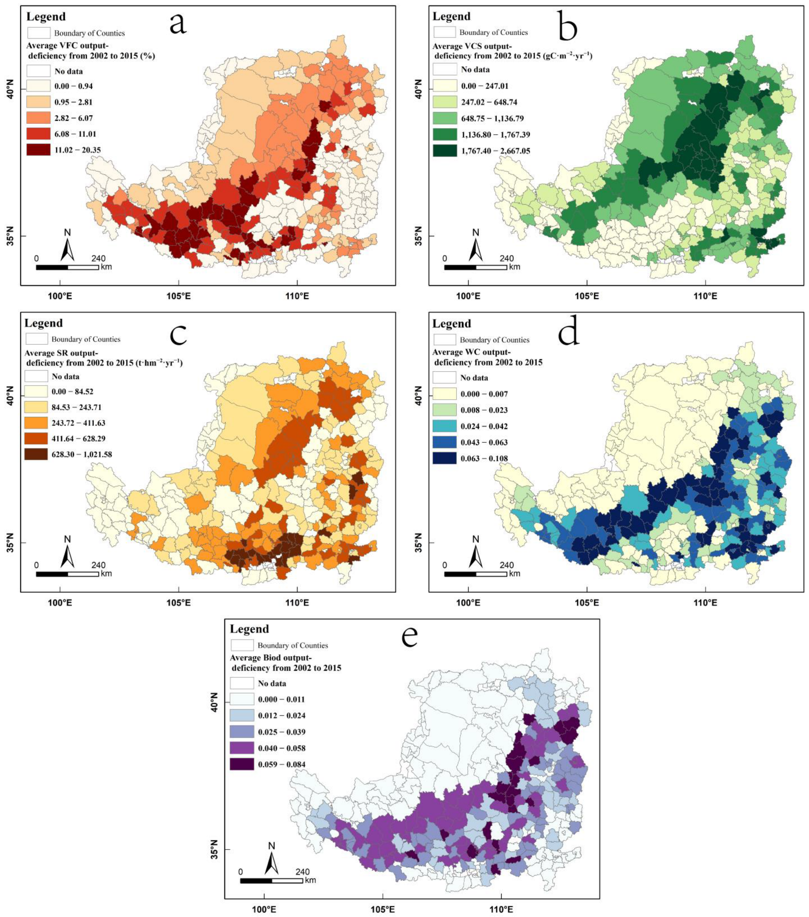
The ecosystem of LP has been greatly restored after the implementation of SLCP and the ecological environment in the territory has been greatly improved. Using 2002 as the base period for SLCP implementation, VFC, VCS, SR, WC, and Biod in the region were all enhanced to varying degrees during 2002–2018.

(2)

The EEoSLCP of LP is low and there is still more room for improvement. In terms of the temporal variation of EEoSLCP, although EEoSLCP has been maintained at a low level, it has generally shown a fluctuating upward trend. In terms of the time-series dynamic evolution of EEoSLCP, there were marked variations in the EEoSLCP between LP counties, with obvious polarization, and a “bimodal” evolution pattern of “low–low clustering and high–high clustering”, which is similar to “club convergence”, is gradually developed with time.

(3)

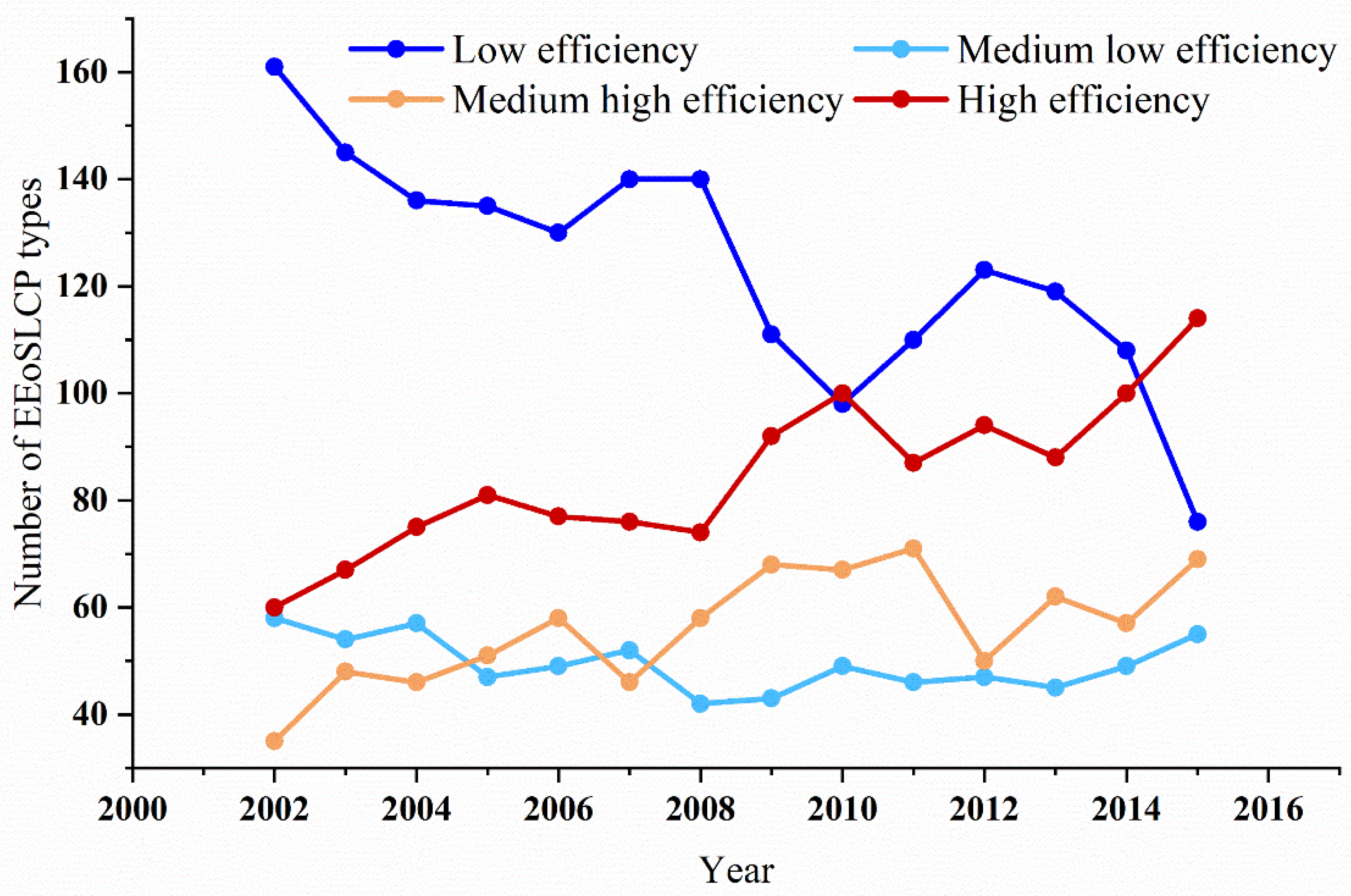
The EEoSLCP in the LP is spatially distributed with regular differences. In terms of spatial distribution, high-efficiency counties are mainly concentrated in the eastern, southern, and western regions, while low-efficiency counties are mainly concentrated in the central, northern, and western regions, and the overall spatial distribution of eco-efficiency is gradually decreasing from southeast to northwest, and from south to north. In terms of spatial change, the number of high-efficiency and medium-high efficiency counties is increasing, while the number of low-efficiency counties is decreasing.

(4)

The EEoSLCP in each county of the LP has a strong spatial dependence and a relatively stable trend in terms of time. In terms of local autocorrelation, the EEoSLCP in each county of the LP shows two correlation trends: “H-H” cluster and “L-L” cluster. H-H clusters are mainly concentrated in the western, southern, and northeastern regions, while L-L clusters are mainly concentrated in the central, northern, and northeastern regions. In terms of spatial and temporal changes, the H-H cluster area is expanding and the L-L cluster area is shrinking.

5.2. Policy Implication

The results of this study can provide three policy implications for the implementation of ERPs around the world. The details are as follows:

(1)

Do the top-level strategy for the implementation of ERPs. Through scientific demonstration, reasonable planning, and farmers’ will, determine the ERPs’ implementation area and, on this basis, determine the ERPs’ implementation tree species according to the natural conditions of local vegetation growth. For example, the EEoSLCP in the northwestern part of the LP is low due to improper selection of SLCP tree species and, in order to improve eco-efficiency, drought-tolerant shrubs (grasses) should be planted and the original vegetation restored in this area.

(2)

Establish a dynamic evaluation mechanism for the eco-effects and ecological efficiency of ERPs, increase the matching of effect and efficiency, and improve the efficiency of resource utilization. For example, in order to improve the EEoSLCP, the SLCP input should be reduced for the central and western counties of the LP, and increased for the eastern and southern counties of the LP.

(3)

Set up a typical example of a successful ecological restoration area to play a demonstration and guiding role. In the implementation of ERPs, it is necessary to make good use of the spatial dependence between neighboring regions, strengthen cooperation and communication between regions, and build an ecological restoration community. For example, in the LP region, H-H cluster type counties should continue to make use of the agglomeration advantages of strong alliances to move towards the goal of higher ecological efficiency of the SLCP, promote the high-quality development of projects, and play a leading role in demonstration; L-H outlier type counties should proactively learn from neighboring high-efficiency counties about SLCP management techniques and experiences. In the implementation of the SLCP, the L-L cluster type counties in the northwest need to base their strategy on local resource endowment and natural conditions, plan tree planting areas, follow the principle of tree species suitability, plant trees in places suitable for tree growth, plant shrubs in places suitable for shrub growth, and reasonably choose trees and shrubs to be planted together to create a compound ecosystem of multiple symbiosis. Meanwhile, the L-L cluster type counties in the center need to reduce land inputs to avoid wasting resources; H-L cluster type counties, while continuing to maintain their own ecological efficiency of the SLCP, should also make use of their accumulated experience of SLCP implementation to guide neighboring low efficiency counties, jointly improve the ecological efficiency of SLCP, and be a good role model.

References

- Bryan, B.A.; Gao, L.; Ye, Y.; Sun, X.; Connor, J.D.; Crossman, N.D.; Stafford-Smith, M.; Wu, J.; He, C.; Yu, D.; et al. China’s Response to a National Land-System Sustainability Emergency. Nature 2018, 559, 193–204. [Google Scholar] [CrossRef] [PubMed]
- Sun, Y.; Ding, W.; Yang, Z.; Yang, G.; Du, J. Measuring China’s Regional Inclusive Green Growth. Sci. Total Environ. 2020, 713, 136367. [Google Scholar] [CrossRef]
- Liu, J.; Li, S.; Ouyang, Z.; Tam, C.; Chen, X. Ecological and Socioeconomic Effects of China’s Policies for Ecosystem Services. Proc. Natl. Acad. Sci. USA 2008, 105, 9477–9482. [Google Scholar] [CrossRef] [PubMed] [Green Version]
- Yin, R.; Yin, G.; Li, L. Assessing China’s Ecological Restoration Programs: What’s Been Done and What Remains to Be Done? Environ. Manag. 2010, 45, 442–453. [Google Scholar] [CrossRef] [PubMed]
- Wang, X.; Bennett, J. Policy Analysis of the Conversion of Cropland to Forest and Grassland Program in China. Environ. Econ. Policy Stud. 2008, 9, 119–143. [Google Scholar] [CrossRef]
- Xian, J.; Xia, C.; Cao, S. Cost–Benefit Analysis for China’s Grain for Green Program. Ecol. Eng. 2020, 151, 105850. [Google Scholar] [CrossRef]
- Bennett, M.T. China’s Sloping Land Conversion Program: Institutional Innovation or Business as Usual? Ecol. Econ. 2008, 65, 699–711. [Google Scholar] [CrossRef] [Green Version]
- Lu, G.; Yin, R. Evaluating the Evaluated Socioeconomic Impacts of China’s Sloping Land Conversion Program. Ecol. Econ. 2020, 177, 106785. [Google Scholar] [CrossRef]
- Chen, C.; Park, T.; Wang, X.; Piao, S.; Xu, B.; Chaturvedi, R.K.; Fuchs, R.; Brovkin, V.; Ciais, P.; Fensholt, R.; et al. China and India Lead in Greening of the World through Land-Use Management. Nat. Sustain. 2019, 2, 122–129. [Google Scholar] [CrossRef]
- Li, J.; Peng, S.; Li, Z. Detecting and Attributing Vegetation Changes on China’s Loess Plateau. Agric. For. Meteorol. 2017, 247, 260–270. [Google Scholar] [CrossRef]
- Li, P.; Wang, J.; Liu, M.; Xue, Z.; Bagherzadeh, A.; Liu, M. Spatio-Temporal Variation Characteristics of NDVI and Its Response to Climate on the Loess Plateau from 1985 to 2015. Catena 2021, 203, 105331. [Google Scholar] [CrossRef]
- Chen, Y.; Wang, K.; Lin, Y.; Shi, W.; Song, Y.; He, X. Balancing Green and Grain Trade. Nat. Geosci. 2015, 8, 739–741. [Google Scholar] [CrossRef]
- Jin, F.; Yang, W.; Fu, J.; Li, Z. Effects of Vegetation and Climate on the Changes of Soil Erosion in the Loess Plateau of China. Sci. Total Environ. 2021, 773, 145514. [Google Scholar] [CrossRef] [PubMed]
- Deng, L.; Liu, S.; Kim, D.G.; Peng, C.; Sweeney, S.; Shangguan, Z. Past and Future Carbon Sequestration Benefits of China’s Grain for Green Program. Glob. Environ. Chang. 2017, 47, 13–20. [Google Scholar] [CrossRef]
- Feng, X.; Fu, B.; Lu, N.; Zeng, Y.; Wu, B. How Ecological Restoration Alters Ecosystem Services: An Analysis of Carbon Sequestration in China’s Loess Plateau. Sci. Rep. 2013, 3, 2846. [Google Scholar] [CrossRef] [Green Version]
- Wang, K.; Hu, D.; Deng, J.; Shangguan, Z.; Deng, L. Biomass Carbon Storages and Carbon Sequestration Potentials of the Grain for Green Program-Covered Forests in China. Ecol. Evol. 2018, 8, 7451–7461. [Google Scholar] [CrossRef] [PubMed]
- Wang, B.; Gao, P.; Niu, X.; Sun, J. Policy-Driven China’s Grain to Green Program: Implications for Ecosystem Services. Ecosyst. Serv. 2017, 27, 38–47. [Google Scholar] [CrossRef]
- Wang, Y.; Zhao, J.; Fu, J.; Wei, W. Effects of the Grain for Green Program on the Water Ecosystem Services in an Arid Area of China-Using the Shiyang River Basin as an Example. Ecol. Indic. 2019, 104, 659–668. [Google Scholar] [CrossRef]
- Wang, C.; Ouyang, H.; Maclaren, V.; Yin, Y.; Shao, B.; Boland, A.; Tian, Y. Evaluation of the Economic and Environmental Impact of Converting Cropland to Forest: A Case Study in Dunhua County, China. J. Environ. Manag. 2007, 85, 746–756. [Google Scholar] [CrossRef]
- Chen, X.; Lupi, F.; Viña, A.; He, G.; Liu, J. Using Cost-Effective Targeting to Enhance the Efficiency of Conservation Investments in Payments for Ecosystem Services. Conserv. Biol. 2010, 24, 1469–1478. [Google Scholar] [CrossRef]
- Ning, J.; Zhang, D.; Yu, Q. Quantifying the Efficiency of Soil Conservation and Optimized Strategies: A Case-Study in a Hotspot of Afforestation in the Loess Plateau. Land Degrad. Dev. 2021, 32, 1114–1126. [Google Scholar] [CrossRef]
- Lu, Y.; Yao, S.; Ding, Z.; Deng, Y.; Hou, M. Did Government Expenditure on the Grain for Green Project Help the Forest Carbon Sequestration Increase in Yunnan, China? Land 2020, 9, 54. [Google Scholar] [CrossRef] [Green Version]
- Zhang, Y.; Zhang, D. Efficiency Measurement and Influencing Factors of Ecological Compensation: A Case Study from Wuqi and Zhidan on the Loess Plateau. Nat. Resour. Res. 2021, 30, 4905–4921. [Google Scholar] [CrossRef]
- Liu, S.; Yao, S. The Effect of Precipitation on the Cost-Effectiveness of Sloping Land Conversion Program: A Case Study of Shaanxi Province, China. Ecol. Indic. 2021, 132, 108251. [Google Scholar] [CrossRef]
- Neto, J.Q.F.; Walther, G.; Bloemhof, J.; Van Nunen, J.; Spengler, T. A Methodology for Assessing Eco-Efficiency in Logistics Networks. Eur. J. Oper. Res. 2009, 193, 670–682. [Google Scholar] [CrossRef] [Green Version]
- Wang, Y.; Zhang, T.; Yao, S.; Deng, Y. Spatio-Temporal Evolution and Factors Influencing the Control Efficiency for Soil and Water Loss in the Wei River Catchment, China. Sustainability 2019, 11, 216. [Google Scholar] [CrossRef] [Green Version]
- Li, G.; Sun, S.; Han, J.; Yan, J.; Liu, W.; Wei, Y.; Lu, N.; Sun, Y. Impacts of Chinese Grain for Green Program and Climate Change on Vegetation in the Loess Plateau during 1982–2015. Sci. Total Environ. 2019, 660, 177–187. [Google Scholar] [CrossRef]
- Li, Z.; Zheng, F.; Liu, W.; Flanagan, D.C. Spatial Distribution and Temporal Trends of Extreme Temperature and Precipitation Events on the Loess Plateau of China during 1961–2007. Quat. Int. 2010, 226, 92–100. [Google Scholar] [CrossRef]
- Wang, L.; Shao, M.; Wang, Q.; Gale, W.J. Historical Changes in the Environment of the Chinese Loess Plateau. Environ. Sci. Policy 2006, 9, 675–684. [Google Scholar] [CrossRef]
- Wang, J.; Liu, Z.; Gao, J.; Emanuele, L.; Ren, Y.; Shao, M.; Wei, X. The Grain for Green Project Eliminated the Effect of Soil Erosion on Organic Carbon on China’s Loess Plateau between 1980 and 2008. Agric. Ecosyst. Environ. 2021, 322, 107636. [Google Scholar] [CrossRef]
- Wu, X.; Wang, S.; Fu, B.; Feng, X.; Chen, Y. Socio-Ecological Changes on the Loess Plateau of China after Grain to Green Program. Sci. Total Environ. 2019, 678, 565–573. [Google Scholar] [CrossRef] [PubMed]
- Amacher, G.S.; Ollikainen, M.; Koskela, E. Economics of Forest Resources; MIT Press: Cambridge, UK, 2009. [Google Scholar]
- Deng, Y.; Cai, W.; Hou, M.; Zhang, X.; Xu, S.; Yao, N.; Guo, Y.; Li, H.; Yao, S. How Eco-Efficiency Is the Forestry Ecological Restoration Program? The Case of the Sloping Land Conversion Program in the Loess Plateau, China. Land 2022, 11, 712. [Google Scholar] [CrossRef]
- Deng, Y.; Jia, L.; Guo, Y.; Li, H.; Yao, S.; Chu, L.; Lu, W.; Hou, M.; Mo, B.; Wang, Y.; et al. Evaluation of the Ecological Effects of Ecological Restoration Programs: A Case Study of the Sloping Land Conversion Program on the Loess Plateau, China. Int. J. Environ. Res. Public Health 2022, 19, 7841. [Google Scholar] [CrossRef] [PubMed]
- Sun, W.; Song, X.; Mu, X.; Gao, P.; Wang, F.; Zhao, G. Spatiotemporal Vegetation Cover Variations Associated with Climate Change and Ecological Restoration in the Loess Plateau. Agric. For. Meteorol. 2015, 209–210, 87–99. [Google Scholar] [CrossRef]
- Wang, S.; Zhao, D.; Chen, H. Government Corruption, Resource Misallocation, and Ecological Efficiency. Energy Econ. 2020, 85, 104573. [Google Scholar] [CrossRef]
- He, L.; Guo, J.; Jiang, Q.; Zhang, Z.; Yu, S. How Did the Chinese Loess Plateau Turn Green from 2001 to 2020? An Explanation Using Satellite Data. Catena 2022, 214, 106246. [Google Scholar] [CrossRef]
- Zhang, D.; Pearse, P.H. Forest Economics; UBC Press: Vancouve, BC, Canada, 2011. [Google Scholar]
- Li, J.; Wang, X.; Shao, M.; Zhao, Y.; Li, X.; Wu, S.; Li, J.; Zhang, R. Simulation of Biomass and Soil Desiccation of Robinia Pseudoacacia Forestlands on Semi-Arid and Semi-Humid Regions of China’s Loess Plateau. Chin. J. Plant Ecol. 2010, 34, 330–339. [Google Scholar]
- Qian, C.; Shao, L.; Hou, X.; Zhang, B.; Chen, W.; Xia, X. Detection and Attribution of Vegetation Greening Trend across Distinct Local Landscapes under China’s Grain to Green Program: A Case Study in Shaanxi Province. Catena 2019, 183, 104182. [Google Scholar] [CrossRef]
- Hua, F.; Wang, X.; Zheng, X.; Fisher, B.; Wang, L.; Zhu, J.; Tang, Y.; Yu, D.W.; Wilcove, D.S. Opportunities for Biodiversity Gains under the World’s Largest Reforestation Programme. Nat. Commun. 2016, 7, 12717. [Google Scholar] [CrossRef] [Green Version]
- Wang, F.; Pan, X.; Gerlein-Safdi, C.; Cao, X.; Wang, S.; Gu, L.; Wang, D.; Lu, Q. Vegetation Restoration in Northern China: A Contrasted Picture. Land Degrad. Dev. 2020, 31, 669–676. [Google Scholar] [CrossRef]
- Chen, J.; Fan, W.; Li, D.; Liu, X.; Song, M. Driving Factors of Global Carbon Footprint Pressure: Based on Vegetation Carbon Sequestration. Appl. Energy 2020, 267, 114914. [Google Scholar] [CrossRef]
- Peng, S.; Wen, D.; He, N.; Yu, G.; Ma, A.; Wang, Q. Carbon Storage in China’s Forest Ecosystems: Estimation by Different Integrative Methods. Ecol. Evol. 2016, 6, 3129–3145. [Google Scholar] [CrossRef] [PubMed] [Green Version]
- Xu, L.; Yu, G.; He, N.; Wang, Q.; Gao, Y.; Wen, D.; Li, S.; Niu, S.; Ge, J. Carbon Storage in China’s Terrestrial Ecosystems: A Synthesis. Sci. Rep. 2018, 8, 2806. [Google Scholar] [CrossRef] [PubMed] [Green Version]
- Xu, L.; He, N.; Yu, G. A dataset of carbon density in Chinese terrestrial ecosystems (2010s). Science Data Bank, 29 July 2018. [Google Scholar] [CrossRef]
- Renard, K.G. Predicting Soil Erosion by Water: A Guide to Conservation Planning with the Revised Universal Soil Loss Equation (RUSLE); United States Government Printing: Washington, DC, USA, 1997.
- Wischmeier, W.H.; Smith, D.D. Predicting Rainfall Erosion Losses: A Guide to Conservation Planning; Department of Agriculture, Science and Education Administration: Washington, DC, USA, 1978.
- Williams, J.R.; Renard, K.G.; Dyke, P.T. EPIC: A New Method for Assessing Erosion’s Effect on Soil Productivity. J. Soil Water Conserv. 1983, 38, 381–383. [Google Scholar]
- Zhang, H.; Yang, Q.; Li, R.; Liu, Q.; Moore, D.; He, P.; Ritsema, C.J.; Geissen, V. Extension of a GIS Procedure for Calculating the RUSLE Equation LS Factor. Comput. Geosci. 2013, 52, 177–188. [Google Scholar] [CrossRef]
- Cai, C.; Ding, S.; Shi, Z.; Huang, L.; Zhang, G. Study of applying USLE and geographical information system IDRISI to predict soil erosion in small watershed. J. Soil Water Conserv. 2000, 14, 19–24. [Google Scholar]
- Yan, R.; Zhang, X.; Yan, S.; Chen, H. Estimating Soil Erosion Response to Land Use/Cover Change in a Catchment of the Loess Plateau, China. Int. Soil Water Conserv. Res. 2018, 6, 13–22. [Google Scholar] [CrossRef]
- Wu, X.; Wang, S.; Fu, B.; Liu, Y.; Zhu, Y. Land Use Optimization Based on Ecosystem Service Assessment: A Case Study in the Yanhe Watershed. Land Use Policy 2018, 72, 303–312. [Google Scholar] [CrossRef]
- Kong, L.; Zheng, H.; Rao, E.; Xiao, Y.; Ouyang, Z.; Li, C. Evaluating Indirect and Direct Effects of Eco-Restoration Policy on Soil Conservation Service in Yangtze River Basin. Sci. Total Environ. 2018, 631–632, 887–894. [Google Scholar] [CrossRef]
- Liu, W.; Liu, J.; Kuang, W. Spatiotemporal patterns of soil protection effect of the Grain for Green Project in northern Shaanxi. Acta Geogr. Sin. 2019, 74, 1835–1852. [Google Scholar]
- Carreño, L.; Frank, F.C.; Viglizzo, E.F. Tradeoffs between Economic and Ecosystem Services in Argentina during 50 Years of Land-Use Change. Agric. Ecosyst. Environ. 2012, 154, 68–77. [Google Scholar] [CrossRef]
- Liu, Y.; Lü, Y.; Jiang, W.; Zhao, M. Mapping Critical Natural Capital at a Regional Scale: Spatiotemporal Variations and the Effectiveness of Priority Conservation. Environ. Res. Lett. 2020, 15, 124025. [Google Scholar] [CrossRef]
- Duan, Y.; Di, B.; Ustin, S.L.; Xu, C.; Xie, Q.; Wu, S.; Li, J.; Zhang, R. Changes in Ecosystem Services in a Montane Landscape Impacted by Major Earthquakes: A Case Study in Wenchuan Earthquake-Affected Area, China. Ecol. Indic. 2021, 126, 107683. [Google Scholar] [CrossRef]
- Barral, M.P.; Oscar, M.N. Land-Use Planning Based on Ecosystem Service Assessment: A Case Study in the Southeast Pampas of Argentina. Agric. Ecosyst. Environ. 2012, 154, 34–43. [Google Scholar] [CrossRef]
- Banker, R.D.; Charnes, A.; Cooper, W.W. Some Models for Estimating Technical and Scale Inefficiencies in Data Envelopment Analysis. Manag. Sci. 1984, 30, 1078–1092. [Google Scholar] [CrossRef] [Green Version]
- Charnes, A.; Cooper, W.W.; Rhodes, E. Measuring the Efficiency of Decision Making Units. Eur. J. Oper. Res. 1978, 2, 429–444. [Google Scholar] [CrossRef]
- Farrell, M.J. The Measurement of Productive Efficiency. J. R. Stat. Soc. Ser. A 1957, 120, 253–281. [Google Scholar] [CrossRef]
- Parzen, E. On Estimation of a Probability Density Function and Mode. Ann. Math. Stat. 1962, 33, 1065–1076. [Google Scholar] [CrossRef]
- Davis, R.A.; Lii, K.-S.; Politis, D.N. Remarks on Some Nonparametric Estimates of a Density Function. In Selected Works of Murray Rosenblatt; Davis, R.A., Lii, K.-S., Politis, D.N., Eds.; Selected Works in Probability and Statistics; Springer: New York, NY, USA, 2011; pp. 95–100. ISBN 978-1-4419-8339-8. [Google Scholar]
- Anselin, L. Interactive Techniques and Exploratory Spatial Data Analysis. In Regional Research Institute Working Paper, 200; West Virginia University: Morgantown, WV, USA, 1996. [Google Scholar]
- Anselin, L. Local Indicators of Spatial Association—LISA. Geogr. Anal. 1995, 27, 93–115. [Google Scholar] [CrossRef]
- Liu, J.; Liu, M.; Zhuang, D.; Zhang, Z.; Deng, X. Study on Spatial Pattern of Land-Use Change in China during 1995–2000. Sci. China Ser. D-Earth Sci. 2003, 46, 373–384. [Google Scholar]
- Liu, J.; Zhang, Z.; Xu, X.; Kuang, W.; Zhou, W.; Zhang, S.; Li, R.; Yan, C.; Yu, D.; Wu, S.; et al. Spatial Patterns and Driving Forces of Land Use Change in China during the Early 21st Century. J. Geogr. Sci. 2010, 20, 483–494. [Google Scholar] [CrossRef]
- Liu, J.; Kuang, W.; Zhang, Z.; Xu, X.; Qin, Y.; Ning, J.; Zhou, W.; Zhang, S.; Li, R.; Yan, C.; et al. Spatiotemporal Characteristics, Patterns, and Causes of Land-Use Changes in China since the Late 1980s. J. Geogr. Sci. 2014, 24, 195–210. [Google Scholar] [CrossRef]
- Kuang, W.; Zhang, S.; Du, G.; Yan, C.; Wu, S.; Li, R.; Lu, D.; Pan, T.; Ning, J.; Guo, C.; et al. Remotely sensed mapping and analysis of spatio-temporal patterns of land use change across China in 2015–2020. Acta Geogr. Sin. 2022, 77, 1056–1071. (In Chinese) [Google Scholar]
- Xu, J.; Yin, R.; Li, Z.; Liu, C. China’s Ecological Rehabilitation: Unprecedented Efforts, Dramatic Impacts, and Requisite Policies. Ecol. Econ. 2006, 57, 595–607. [Google Scholar] [CrossRef]
- Yin, R.; Yin, G. China’s Primary Programs of Terrestrial Ecosystem Restoration: Initiation, Implementation, and Challenges. Environ. Manag. 2010, 45, 429–441. [Google Scholar] [CrossRef] [PubMed]
- Yu, X. Central–Local Conflicts in China’s Environmental Policy Implementation: The Case of the Sloping Land Conversion Program. Nat. Hazards 2016, 84, 77–96. [Google Scholar] [CrossRef]
- Qu, M.; Liu, G.; Lin, Y.; Driedger, E.; Peter, Z.; Xu, X.; Cao, Y. Experts’ Perceptions of the Sloping Land Conversion Program in the Loess Plateau, China. Land Use Policy 2017, 69, 204–210. [Google Scholar] [CrossRef]
- Trac, C.J.; Harrell, S.; Hinckley, T.M.; Henck, A.C. Reforestation Programs in Southwest China: Reported Success, Observed Failure, and the Reasons Why. J. Mt. Sci. 2007, 4, 275–292. [Google Scholar] [CrossRef]
- Delang, C.O.; Wang, W. Chinese Forest Policy Reforms after 1998: The Case of the Natural Forest Protection Program and the Slope Land Conversion Program. Int. For. Rev. 2013, 15, 290–304. [Google Scholar] [CrossRef]
- He, J.; Sikor, T. Notions of Justice in Payments for Ecosystem Services: Insights from China’s Sloping Land Conversion Program in Yunnan Province. Land Use Policy 2015, 43, 207–216. [Google Scholar] [CrossRef]
- He, J. Governing Forest Restoration: Local Case Studies of Sloping Land Conversion Program in Southwest China. For. Policy Econ. 2014, 46, 30–38. [Google Scholar] [CrossRef]
- He, J. Situated Payments for Ecosystem Services: Local Agencies in the Implementation of the Sloping Land Conversion Programme in Southwest China. Dev. Chang. 2020, 51, 73–93. [Google Scholar] [CrossRef]
- Chen, C.; König, H.J.; Matzdorf, B.; Zhen, L. The Institutional Challenges of Payment for Ecosystem Service Program in China: A Review of the Effectiveness and Implementation of Sloping Land Conversion Program. Sustainability 2015, 7, 5564–5591. [Google Scholar] [CrossRef] [Green Version]
- Liu, J.; Chen, H.; Hou, X.; Zhang, D.; Zhang, H. Time to Adopt a Context-Specific and Market-Based Compensation Scheme for a New Round of the Grain for Green Program. Land Use Policy 2021, 108, 105675. [Google Scholar] [CrossRef]
- Cao, S.; Chen, L.; Shankman, D.; Wang, C.; Wang, X.; Zhang, H. Excessive Reliance on Afforestation in China’s Arid and Semi-Arid Regions: Lessons in Ecological Restoration. Earth-Sci. Rev. 2011, 104, 240–245. [Google Scholar] [CrossRef]
- Donohue, R.J.; Roderick, M.L.; McVicar, T.R. On the Importance of Including Vegetation Dynamics in Budyko’s Hydrological Model. Hydrol. Earth Syst. Sci. 2007, 11, 983–995. [Google Scholar] [CrossRef] [Green Version]
- Jiang, G.; Han, X.; Wu, J. Restoration and Management of the Inner Mongolia Grassland Require a Sustainable Strategy. AMBIO A J. Hum. Environ. 2006, 35, 269–270. [Google Scholar] [CrossRef]
- Cao, S. Why Large-Scale Afforestation Efforts in China Have Failed To Solve the Desertification Problem. Environ. Sci. Technol. 2008, 42, 1826–1831. [Google Scholar] [CrossRef] [Green Version]
- Cao, S.; Tian, T.; Chen, L.; Dong, X.; Yu, X.; Wang, G. Damage Caused to the Environment by Reforestation Policies in Arid and Semi-Arid Areas of China. AMBIO 2010, 39, 279–283. [Google Scholar] [CrossRef]
- Bullock, A.; King, B. Evaluating China’s Slope Land Conversion Program as Sustainable Management in Tianquan and Wuqi Counties. J. Environ. Manag. 2011, 92, 1916–1922. [Google Scholar] [CrossRef]
- Tao, R.; Xu, Z.; Xu, J. Grain for green project, grain policy and sustainable development. Soc. Sci. China 2004, 150, 25–38. (In Chinese) [Google Scholar]
- Xu, J.; Tao, R.; Xu, Z.G. Sloping land conversion program: Cost-effectiveness, structural effect and economic sustainability. China Econ. Q. 2004, 4, 139–162. (In Chinese) [Google Scholar]