A Novel 3D Tree-Modeling Method of Incorporating Small-Scale Spatial Structure Parameters in a Heterogeneous Forest Environment

Abstract

Currently, 3D tree modeling in a highly heterogeneous forest environment remains a significant challenge for the modeler. Previous research has only focused on morphological characteristics and parameters, overlooking the impact of micro-environmental factors (e.g., spatial-structural diversification and habitat heterogeneity) and providing less structural information about the individual tree and decreasing the applicability and authenticity of 3D tree models in a virtual forest. In this paper, we chose a mixed-forest conversion of Chinese fir (Cunninghamia lanceolata) plantations in a subtropical region of China as our study subject and proposed a novel 3D tree-modeling method based on a structural unit (TMSU). Our approach modified traditional rule-based tree modeling (RTM) by introducing a nonlinear mixed-effect model (NLME) to study the coupling response between the spatial structures and morphological characteristics (e.g., tree height (H), height-to-crown base (H_CB), and crown width (CW)) of three dominant trees (e.g., Cunninghamia lanceolata (SM), Machilus pauhoi (BHN), and Schima superba (MH)) and develop a prediction model of the morphological characteristic by incorporating forest-based structural parameters. The results showed that: (1) The NLME model in TMSU was found to better fit the data and predict the morphological characteristics than the OLS model in RTM. As compared to the RTM morphological model, the prediction accuracy of the TMSU model of morphological features was improved by 10.4%, 3.02%, and 17.8%, for SM’s H, H_CB, and CW, respectively; 6.5%, 7.6%, and 8.9% for BHN’s H, H_CB, and CW, respectively; and 13.3%, 15.7%, and 13.4% for MH’s H, H_CB, and CW, respectively. (2) The spatial-structural parameters of crowding ($C_i$), mingling ($M_i$), and dominance ($U_i$) had a significant impact on the morphological characteristics of SM, BHN, and MH in TMSU. The degree of crowding, for example, had a positive relationship with tree height, height-to-crown base, and crown width in SM, BHN, and MH; under the same crowding conditions, mingling was positively correlated with tree crown width in SM, and dominance was positively correlated with tree height but negatively correlated with height-to-crown base in BHN; under the same crowding and mingling, dominance was positively correlated with height-to-crown base in MH. (3) Using 25 scenes based on the value class of $C_i,M_i$ for SM, 25 scenes based on the value class of $C_i,U_i$ for BHN, and 125 scenes based on the value class of $C_i,M_i,U_i$ for MH, we generated the model libraries for the three dominating species based on TMSU. As a result, our TSMU method outperformed the traditional 3D tree-modeling method RTM in a complex and highly heterogeneous spatial structure of a forest stand, and it provided more information concerning the spatial structure based on the neighborhood relationships than the simple morphological characteristics; a higher morphological prediction accuracy with fewer parameters; and the relationship between the spatial-structural parameters and the morphological characteristics of a reference tree.

1. Introduction

The current 3D tree-modeling methods, such as those based on LIDAR point-cloud data and RGB-D images, have high precision but are costly and computationally intensive [1,2,3]. Furthermore, it is not appropriate to reconstruct 3D tree models in a dense and highly heterogeneous forest stand because there is insufficient space to obtain sufficient data. Therefore, 3D tree modeling, based on forestry rules, provides a set of generative rules to create plant organs iteratively, though it requires expertise in botany to manually adjust the many parameters in order to model a specific tree [4]. This method has proven to be an effective and popular method for virtual forest reconstruction [5,6]. For example, functional–structural plant models (FSPMs) require specific parameters to model a tree, such as tree height, diameter at breast height, crown width, and height-to-crown base [7]. Therefore, rule-based tree modeling can be easily controlled by modelers without a computer science background [8]. However, the applicability of rule-based modeling is limited because it is based on only a few parameters and overlooks the influence of micro-environmental factors (e.g., spatial-structure diversification and habitat heterogeneity) in a complex and changing forest ecosystem.

Exploring the coupling response between variables related to the spatial structure and morphological characteristics is vital in 3D tree modeling based on a structural unit in a highly heterogeneous forest environment. However, the current research has mostly focused on the coupling responses between unilateral or incomplete characteristics of the spatial structure and tree-crown attributes. For example, researchers suggested that when mixed with other species, the reference tree changed the typical structural attributes of the crown [9,10,11,12], such as branching patterns [10,13] and the general shape of the crown [11,12,13,14]. These changes could be attributed to the amount of light available, which is the most important resource for which trees compete in a forest canopy [12,13,14,15]. Researchers discovered that trees adjusted the shapes and sizes of their crowns in response to competition with their neighbors under different spatial-structure conditions [16], such as in crowded conditions [17,18]. With the rapid application of airborne laser-scanning techniques, more studies are being conducted at the individual tree level and in a more intelligent direction. For example, Pommerening et al. (2021) introduced the CanopyShotNoise model to analyze the response of the canopy pattern under different forest conditions [19]. Fischer et al. (2020) proposed a new simulation-based approach, the canopy constructor, to quantify the forest structure and infer the allometric-scaling relationship in a crowded environment [20].

Morphological models, such as height–diameter, crown width–diameter, and height-to-crown base height–diameter, are critical components of rule-based 3D tree modeling. The prediction accuracy of a model significantly influences the applicability and authenticity of 3D tree models in a virtual forest. Traditional morphological models have adopted the ordinary least squares (OLS) regression for the simple form and its variables. However, the morphological data from many sample plots have hierarchical structures and may be correlated, which has resulted in biased estimations of the variance of the morphological parameters and invalidated the hypothesis when the parameter estimates were analyzed [21,22]. Lately, the popularity and use of mixed-effect models have increased in forestry and morphological modeling practices [23,24,25]. Researchers have suggested that, as compared to OLS, the nonlinear mixed-effect model (NLME) was more reliable due to its assumption of random and independent observations, as well as the presence of autocorrelations [26,27,28,29].

Therefore, in order to model 3D trees in a spatially diverse and heterogeneous forest environment, we chose a mixed forest of Chinese fir (Cunninghamia lanceolata) as our subject, which was based on a typical mixed forest stand in a subtropical region of China. The following two aspects were explored in this study: (1) to develop the morphological characteristics (e.g., tree height, height-to-crown base, and crown width) of the model at the individual tree level and with highly heterogeneous spatial structures by introducing a NLME model and (2) to optimize the traditional rule-based 3D tree-modeling method by incorporating individual parameters of spatial structures based on a small-scale forest stand in order to develop a new dominant species’ model library under heterogeneous forest conditions.

2. Materials and Methods

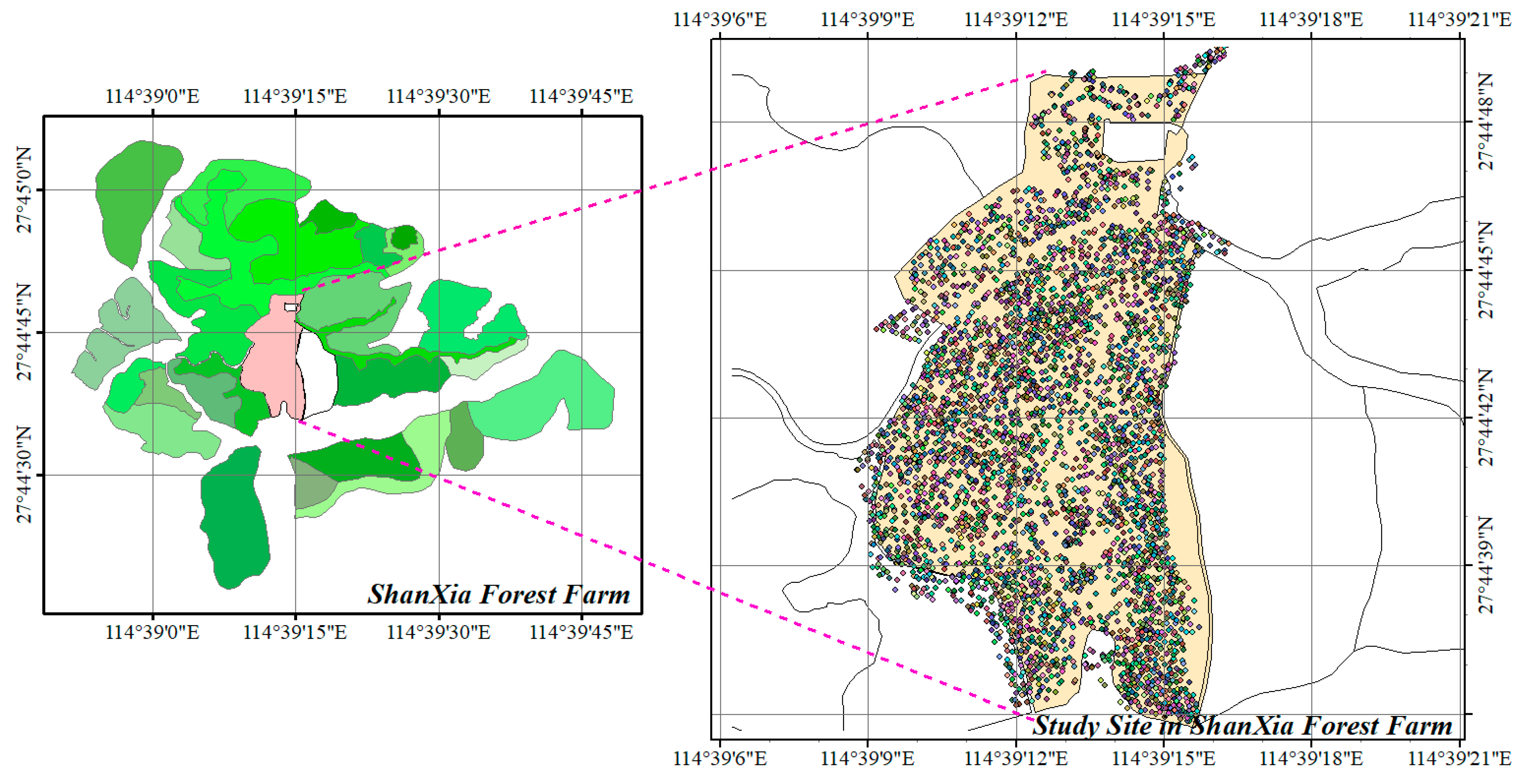
2.1. Study Areas

Our study site was located in the ShanXia Forest Farm in Jiangxi Province in Southern China (27°44′45″ N, 114°39′15″ E) (see Figure 1). The site has a mid-subtropical climate and a mean annual temperature of 19.15 °C, with the highest temperature of 40.3 °C occurring in June and July and the lowest temperature of −2.1 °C occurring in February. Furthermore, annual precipitation totaled 1722.3 mm, with the majority of the precipitation falling in April, May, and June. The annual photoperiod was 1657.4 h, with the longest photoperiod occurring in July, August, September, and October and the shortest occurring in January and February. The Chinese fir mixed plantations selected in this study were established in 1986 with an initial planting spacing of 1m × 1m. Thinning measures were taken when the plantations were 13 years and 20 years old. The first thinning measure was to reduce the intraspecific competition for resource by increasing the growth space and the second thinning measure was to fell the low-quality trees and replant broadleaved trees, such as Machilus pauhoi and Schima superba, which are high-value, fire-resistant trees. During the development of the mixed plantations, some Chinese firs died, allowing companion species or generations to develop in natural succession, such as Vernicia fordii, Liquidambar formosana Hance, Paulowinia fortune, Sapium discolorr, Castanopsis fargesii, etc.

2.2. Data Collection

The data was acquired from 5 ha sample plots of a planted mixed forest dominated by Cunninghamia lanceolata, Machilus pauhoi, and Schima superba in March and April 2022 (Figure 2). To accurately locate the trees, the plot was divided into 10 subplots of 100 m × 50 m each (Figure 2). Tree height (H), height-to-crown base (${\mathrm{H}}_{\mathrm{C}\mathrm{B}}$), diameter at breast height (DBH), and crown width (CW) were measured for all trees with a diameter at breast height of (DBH) ≥ 5 cm, and their locations were recorded using a total station (TOPCON-GTS-602AF). Crown width was computed as the arithmetic mean of two crown widths obtained from measurements of four crown radii, representing two azimuths [30]. The first azimuth was defined as the direction from the subject tree to the center of the measurement plot; the second azimuth was perpendicular to the first. In each quadrant, the crown radii were measured as the horizontal distance from the center of the tree bole to the greatest extent of the crown from the bole. The branch tip was located by vertical sighting with a clinometer [31]. Figure 2 depicts a distribution map of the tree species, and each tree population was assigned three layer classes, based on tree height, to select the dominant trees: upper layer trees were H ≥ 20 m; middle layer trees were 10 m ≤ H < 20 m; and lower layer trees were 1.3 m ≤ H < 10 m.

To eliminate edge effects and improve the accuracy of the spatial-structure parameters (SSP), we established a 5 m buffer zone around the plot. In the statistical analysis, only the trees in the reduced window (X, Y) = (300 m × 200 m, except (0 m–100 m, 0–50), (200 m–300 m, 0 m–50 m)) were used as reference trees, and the individual trees in the buffer zone were only considered to be the nearest neighbors of the trees in the reduced window [32]. This edge correction enabled the individual evaluation of each tree to determine whether all n-nearest-neighbors were actually located within the plot.

2.3. Data Analysis

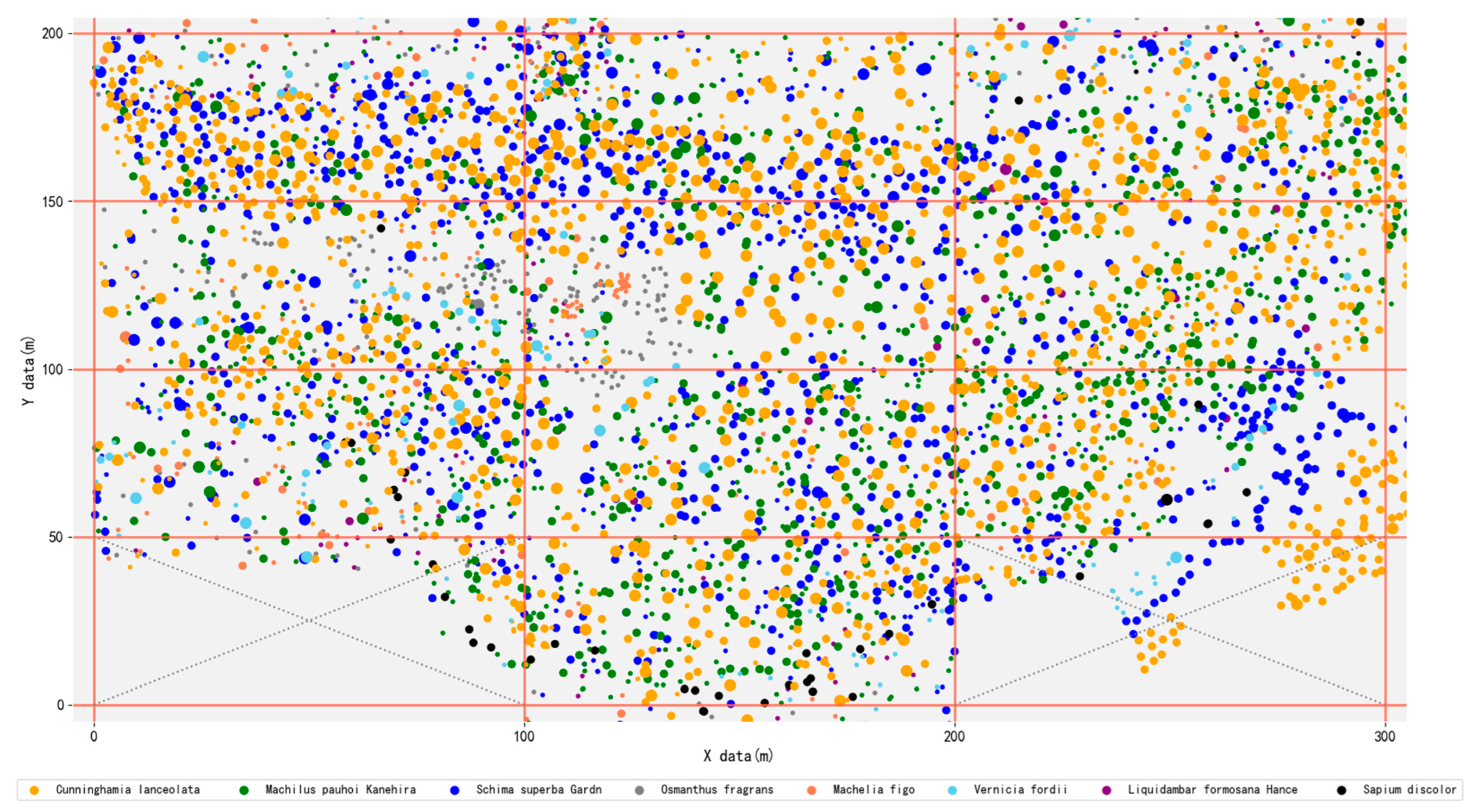
2.3.1. Identification of Dominant Populations for 3D Tree Modeling by the Important Value Index

The importance value (IV) of a species was defined as the average of its relative density (RD), relative frequency (RF), and relative dominance (Rd) and was calculated using the quadratic method [33] for each layer of the planted mixed forest. A total of 32 tree species belonging to 30 genera and 21 families were identified in the planted mixed forest. The total stand density (DBH ≥ 5 cm) was nearly 996.8 trees/ha, with a total basal area of 161.2 m²/ha.

Table 1. IV and characteristics of eight dominant tree populations in the planted mixed forest.

Species	Density	IV (%)				Stand Characteristics
	(Trees ha−1)	Upper Layer	Median Layer	Lower Layer	All	DBH	Height	Basal Area	Dominant Height (m)
						(cm)	(m)	(m2)
Cunninghamia lanceolata (Lamb.) Hook.	273.0	14.57 ± 7.14	15.13 ± 5.19	3.28 ± 1.86	17.18 ± 3.74	24.86 ± 8.91	16.50 ± 5.40	80.83	26.8
Machilus pauhoi Kanehira	252.6	2.53 ± 1.68	10.38 ± 2.73	7.04 ± 3.13	11.13 ± 3.44	13.82 ± 8.25	10.63 ± 3.83	25.72	23.5
Schima superba Gardn. et Champ.	259.0	1.21 ± 1.25	12.78 ± 4.21	4.32 ± 1.88	12.39 ± 4.39	15.32 ± 7.02	11.85 ± 3.55	27.67	23.4
Osmanthus fragrans (Thunb.) Lour.	62.0	0.00 ± 0.00	0.00 ± 0.00	1.82 ± 3.56	1.65 ± 2.94	10.37 ± 3.31	5.74 ± 1.12	2.88	8.2
Machelia figo (Lour.) Spreng.	48.0	0.07 ± 0.21	0.81 ± 0.90	1.12 ± 1.35	1.59 ± 1.60	13.69 ± 8.03	9.30 ± 3.76	4.36	18.8
Vernicia fordii (Hemsl.) Airy Shaw	35.6	0.21 ± 0.55	1.34 ± 1.23	0.41 ± 0.74	1.52 ± 1.65	22.60 ± 9.47	14.21 ± 3.40	7.54	21.1
Liquidambar formosana Hance	27.0	0.03 ± 0.09	0.63 ± 0.90	0.74 ± 0.86	1.24 ± 1.43	16.26 ± 7.63	12.19 ± 3.45	3.01	18.2
Sapium discolor (Champ. ex Benth.) Muell. Arg.	21.8	0.00 ± 0.00	0.91 ± 1.76	0.13 ± 0.40	0.74 ± 1.21	22.22 ± 7.83	13.33 ± 1.92	4.21	15.4

Notes: IVs, DBH, and Height are mean ± SD; the upper layer was tree height (H) ≥ 20 m; the middle layer was 10 m ≤ tree height (H) < 20 m; and the lower layer was 1.3 m tree height (H) < 10 m.

shows the IVs of the forest’s eight dominant tree populations. Cunninghamia lanceolata, Machilus pauhoi, and Schima superba accounted for 88.24% of the total stand density, and their IVs were clearly superior to those of the other tree species in different stand layers. As a result, they were identified as the dominant populations in the forest for 3D tree modeling (Table 1).

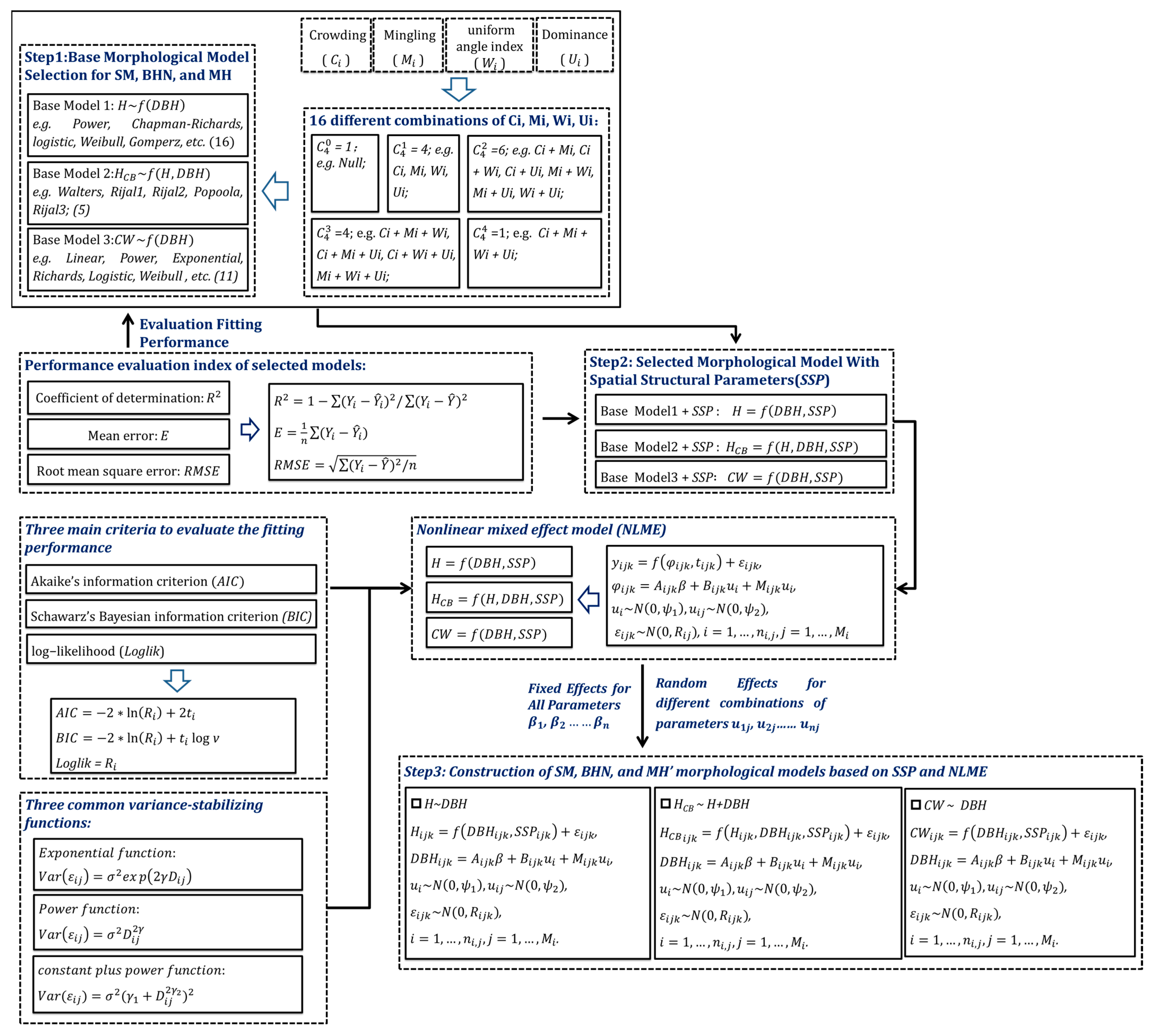
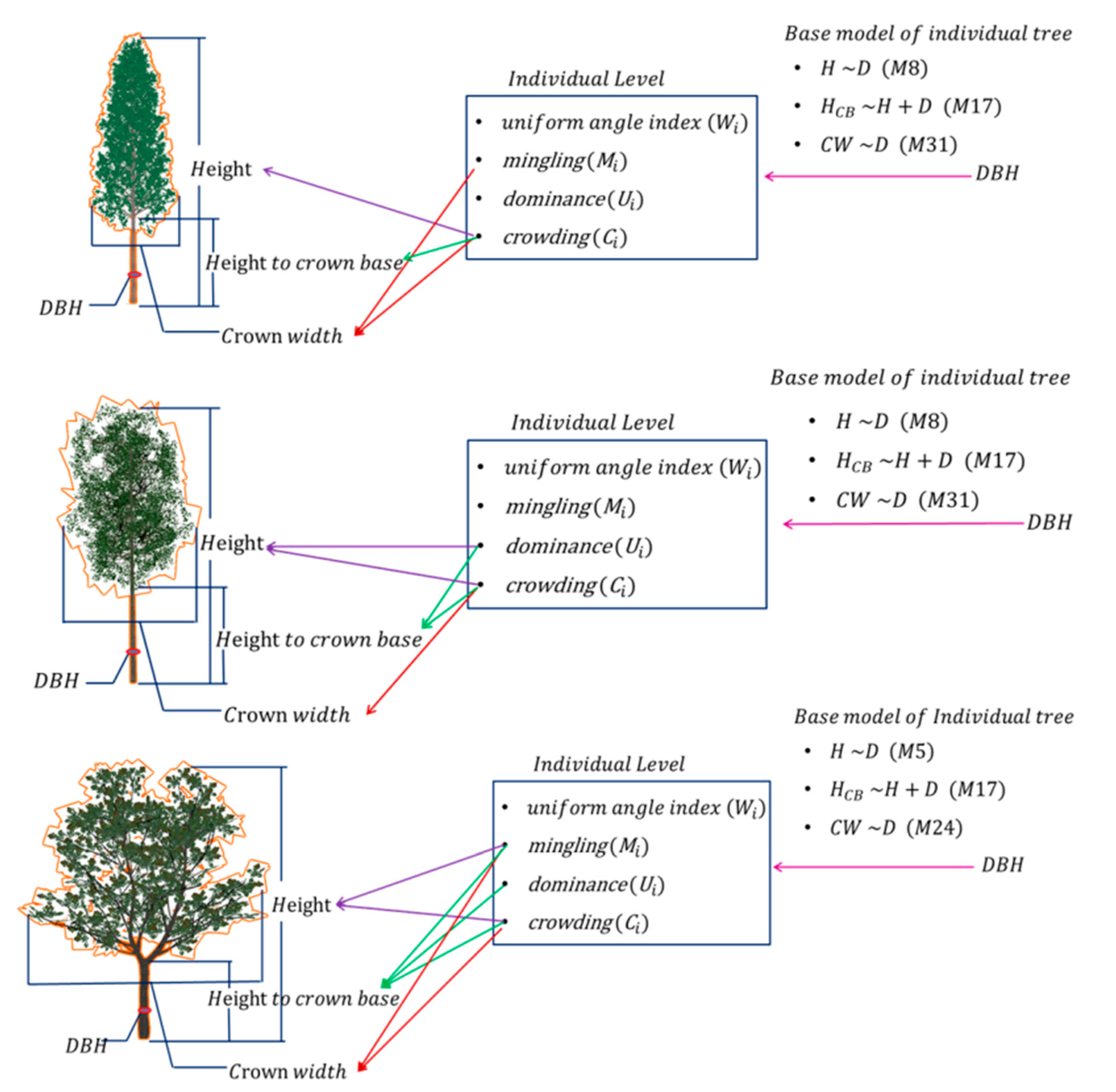
2.3.2. Nonlinear Mixed-Effect Morphological Model of Three Predominant Trees

(1) Base morphological model selection.

In this paper, we chose 16 H~DBH models, 5 HCB~H and DBH models, and 11 CW~DBH models from the literature for appraisal as the base models [27,28,34,35]. These candidate base models were fitted to the 10 plot data (5 ha) using nonlinear least squares regression. The three statistical variables (e.g., coefficient of determination (R²), mean error (E), root-mean-squared error (RMSE)) were used to evaluate the performance of the base models (see Figure 3). The H, H_CB, and CW base models evaluated in this study are shown in

Table 2. Base model selection: H is the total tree height (m), DBH is the diameter at breast height (cm), H_CB is the height-to-crown base (m), and CW is the crown width (m); a, b, and c are the parameters of the model. M1~M32 represents the formulae of the morphological characteristic models.

Model	Formula	Model Form	Model	Formula	Model Form
M1	H~1.3 + DBH2/(a∗DBH + b)2	Naslund	M17	HCB~H/(1 + exp(a + b∗DBH))	Walters
M2	H~1.3 + a∗DBH/(1 + DBH)b	Curtis	M18	HCB~H/(1 + exp(a + b∗DBH))1/2	Rijal 1
M3	H~1.3 + a∗exp(−b/DBH)	Schumacher	M19	HCB~H/(1 + exp(a + b∗DBH))1/6	Rijal 2
M4	H~1.3 + a∗(1 − exp(−b∗DBH))	Meyer	M20	HCB~H/(a + exp(−b∗DBH))	Popoola
M5	H~1.3 + a∗DBHb	Power	M21	HCB~H/(1 − a∗exp(−b∗DBH))	Rijal 3
M6	H~1.3 + a∗DBH/(b + DBH)	Michaelis-Menten	M22	CW~a + b∗DBH	Linear
M7	H~1.3 + exp(a − b/(DBH + 1))	Wykoff	M23	CW~a + b∗DBH + c∗DBH2	Quadratic
M8	H~1.3 + a∗((1 − exp(-b∗DBH)))	Chapman–Richards	M24	CW~a∗DBHb	Power
M9	H~1.3 + DBH2/(a∗DBH2 + b∗DBH + c)	Prodan	M25	CW~a∗(1−exp(−b∗DBH))	Monomolecular
M10	H~1.3 + a/(1 + b∗exp(−c∗DBH))	logistic	M26	CW~(DBH/(a + b∗DBH))2	Hossfeld I
M11	H~1.3 + a∗(1-exp(−b∗DBHc))	Weibull	M27	CW~a∗(b)DBH	Compound
M12	H~1.3 + a∗exp(−b∗exp(−c∗DBH))	Gomperz	M28	CW~exp(a + b∗DBH)	Growth
M13	H~1.3 + a∗DBH(b∗DBH−c)	Sibbesen	M29	CW~a∗exp(b∗DBH)	Exponential
M14	H~1.3 + a∗exp(−b∗DBH−c)	Korf	M30	CW~a∗(1 − exp(−b∗DBH))	Richards
M15	H~1.3 + a∗exp(−b/(DBH + c))	Ratkowsky	M31	CW~a/(1 + b∗exp(−c∗DBH))	Logistic
M16	H~1.3 + a/(1 + 1/(b∗DBHc))	Hossfeld IV	M32	CW~a∗(1 − exp(−b∗DBH))	Weibull

.

(2) Additional predictor variables.

A structural unit was defined as a neighborhood consisting of a focal tree and its four nearest neighbors [36]. In a mixed forest, tree size (DBH or crown), tree crowding, tree species, and tree distribution in space were used to describe any structural unit synchronously. These variables were easily expressed by a set of structural stand parameters: $W_i$, $M_i$, $C_i$, and $U_i$ [37,38]. Therefore, there were 16 different combinations of $W_i$, $M_i$, $C_i$, and $U_i$ for selecting the best performing model according to two rules: higher prediction accuracy and lower computational cost (see Figure 3).

$$W_i=\frac{1}{n}{\sum }_{j=1}^n{Z}_{ij},Z_{ij}=\left\{\begin{array}{l}\begin{array}{cc}1,& if \alpha -angle is smaller than {\alpha }_0\end{array}\\ \begin{array}{cc}\begin{array}{cc}0,\hspace{1em}\hspace{1em}& otherwise\end{array}& \end{array}\end{array}\right.$$

(1)

where $W_i$ is defined as the proportion of angles $\alpha$ smaller than the standard angle ${\alpha }_0$ (72°) and reflects the degree of uniformity of tree distribution.

$$M_i=\frac{1}{n}{\sum }_{j=1}^n{V}_{ij},V_{ij}=\left\{\begin{array}{l}\begin{array}{cc}1,& if neighbor j is not the same species as reference tree i\end{array}\\ \begin{array}{cc}\begin{array}{cc}0,\hspace{1em}\hspace{1em}\hspace{1em}\hspace{1em}& otherwise\end{array}& \end{array}\end{array}\right.$$

(2)

where $M_i$ is defined as the proportion of the four nearest neighbors that are of a different species than reference tree i, and it reflects the spatial segregation of different species in a multispecies forest.

$$U_i=\frac{1}{n}{\sum }_{j=1}^n{K}_{ij},K_{ij}=\left\{\begin{array}{c}\begin{array}{cc}0,& if neighbor j is smaller than reference tree i\end{array}\\ \begin{array}{cc}\begin{array}{ccc}1,& & otherwise\end{array}& \end{array}\end{array}\right.$$

(3)

where $U_i$ is defined as the degree of DBH differentiation in this paper and represents the relationship between the size of the reference tree i and its four nearest neighbors.

$$C_i=\frac{1}{n}{\sum }_{j=1}^n{P}_{ij},P_{ij}=\left\{\begin{array}{c}\begin{array}{cc}1,& if average crowns of neighbor j and reference tree i\end{array}\\ is smaller than that of reference i\\ \begin{array}{cc}\begin{array}{ccc}0,& & otherwise\end{array}& \end{array}\end{array}\right.$$

(4)

where $C_i$ reflects the relationship between the canopy of the reference tree i and its four nearest neighbors and can reveal the degree of crowding of the reference tree i.

(3) Construction of mixed-effect morphological model.

We have incorporated the fixed effects for all parameters in the morphological characteristics models and compared different combinations of all parameters with random effects in the model to identify the parameters that needed to be included, according to the value of the Akaike information criteria (AIC) and Schwarz’s Bayesian information criterion (BIC), which were the main criteria for evaluating the fitting performance. In order to solve the problem of heteroscedasticity in the morphological models, we used three typical variance-stabilizing functions (e.g., exponential function, power function, and constant-plus-power function) (4–6) (Figure 3) and selected the best-performing function based on the AIC and the log-likelihood (Loglik) values (see Figure 3).

The graphic exploration and correlational analysis were used for evaluation of the contributions of the covariate predictors to the H, H_CB, and CW models. All analyses were conducted using R, version 4.1.2. The best-performing model was selected to include additional covariate predictors for formulations of the H, H_CB, and CW mixed-effect models.

(4) Assessment and analysis of morphological models

The main differences between rule-based tree modeling (RTM) and 3D tree modeling based on a structural unit (TMSU) were the morphological models’ parameter-estimation model and whether the tree modeling considered the spatial structure. In general, the parameter estimation in a traditional morphological model in RTM was based on the ordinary least squares (OLS) model, whereas in TMSU, it was based on a nonlinear mixed-effect model (NLME). In order to validate the feasibility and superiority of the morphological models in TMSU for 3D tree modeling, statistics (R², E, RMSE) and a residual plot of three dominant tree-based morphological models were applied to assess and analyze the morphological models based on OLS and NLME.

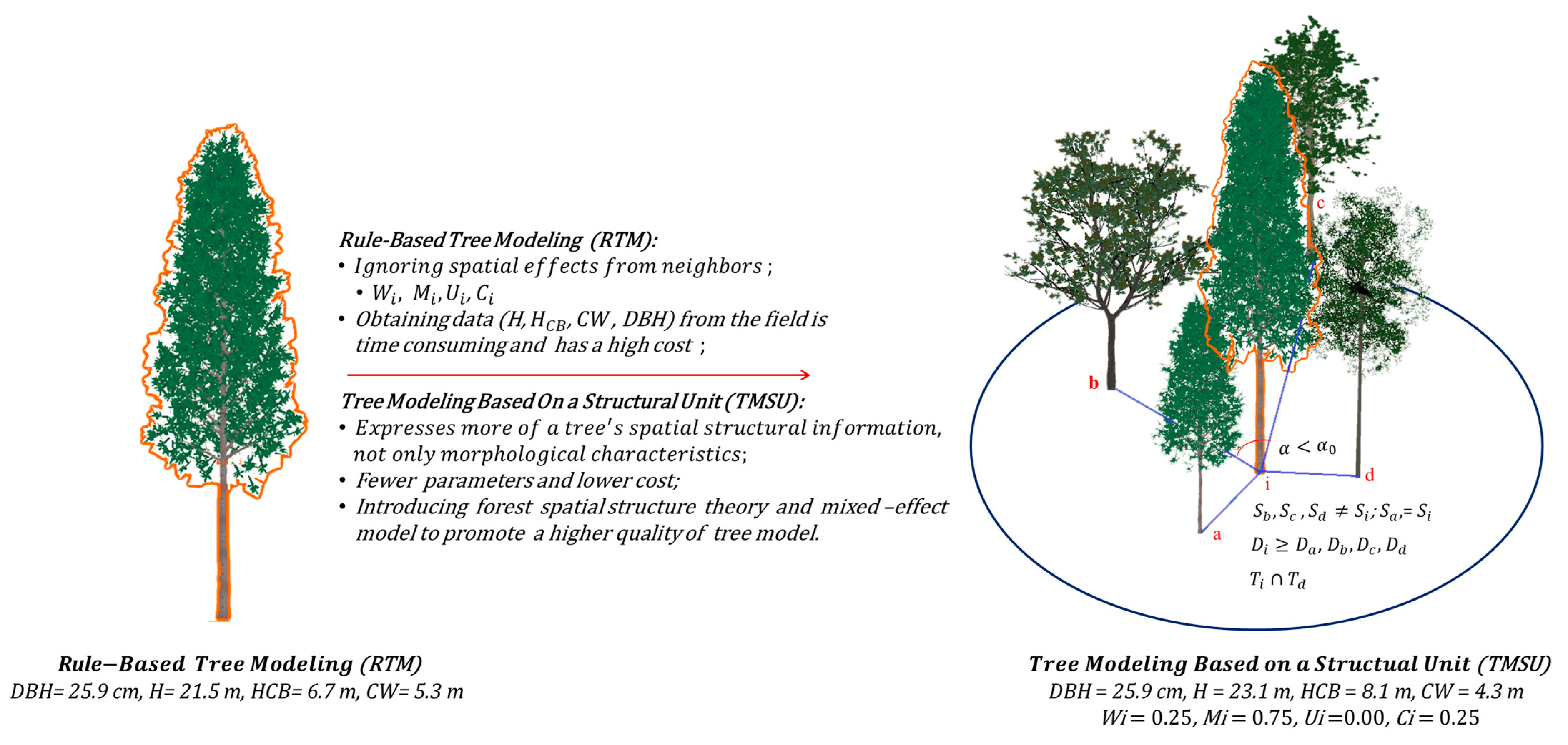
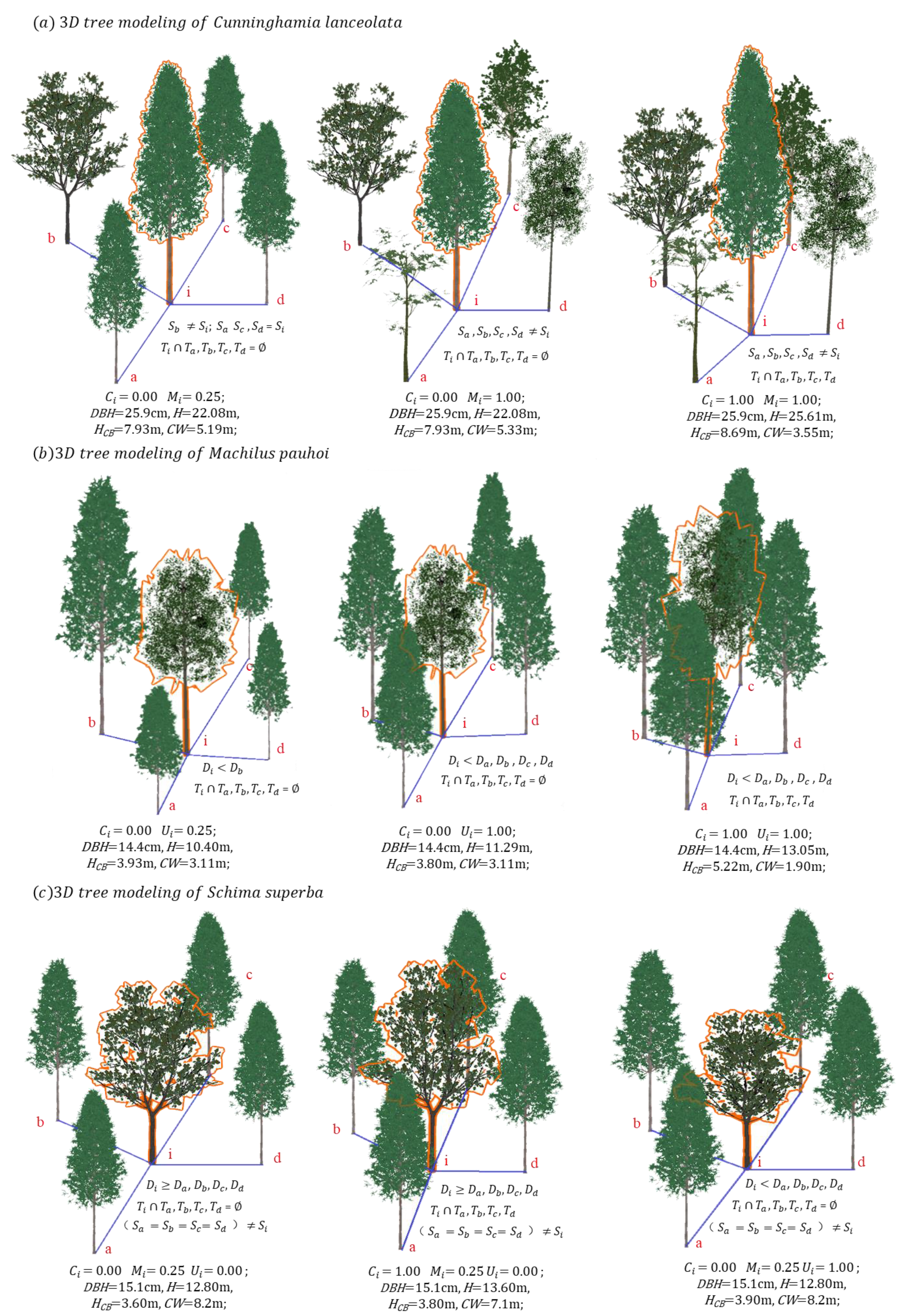
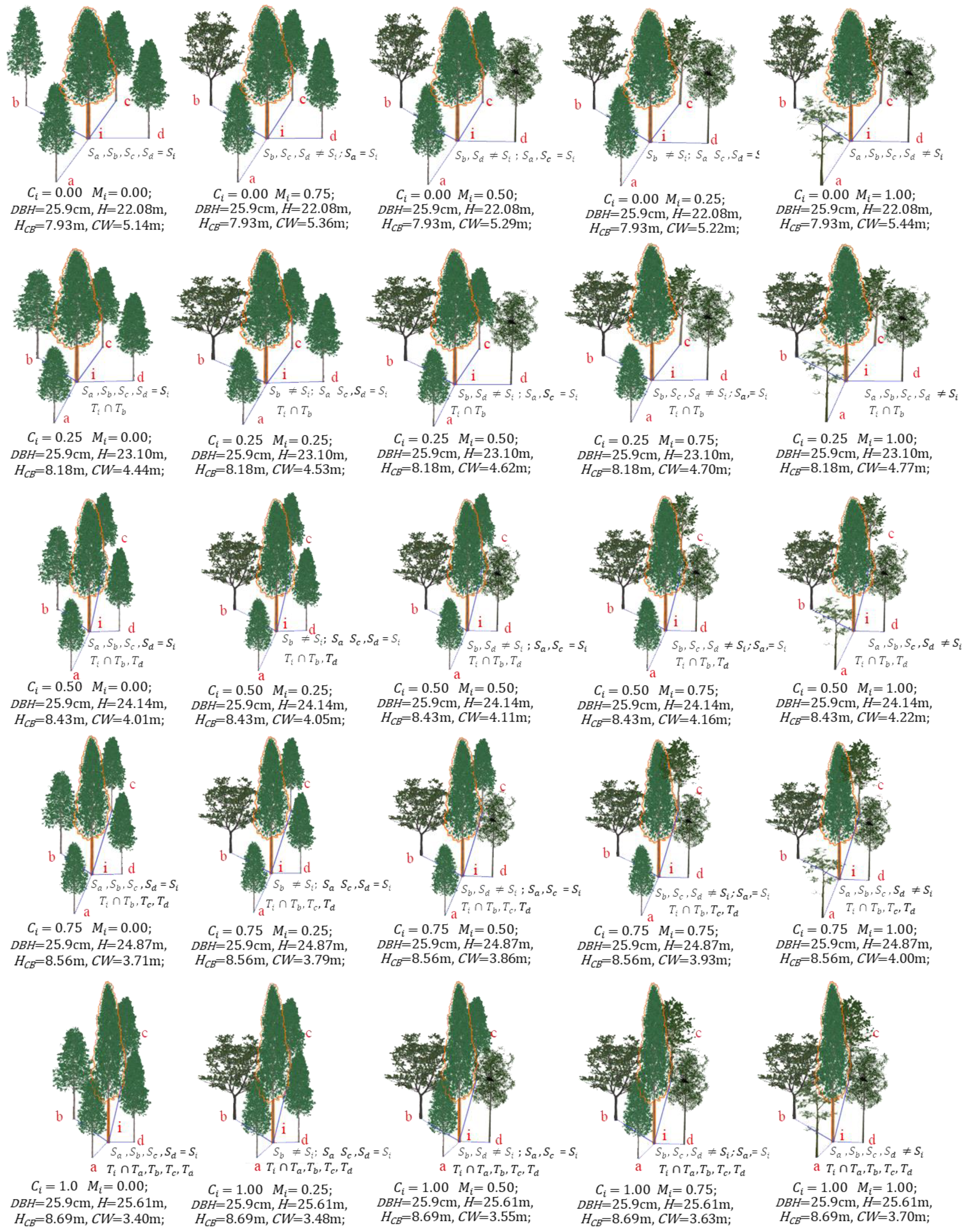
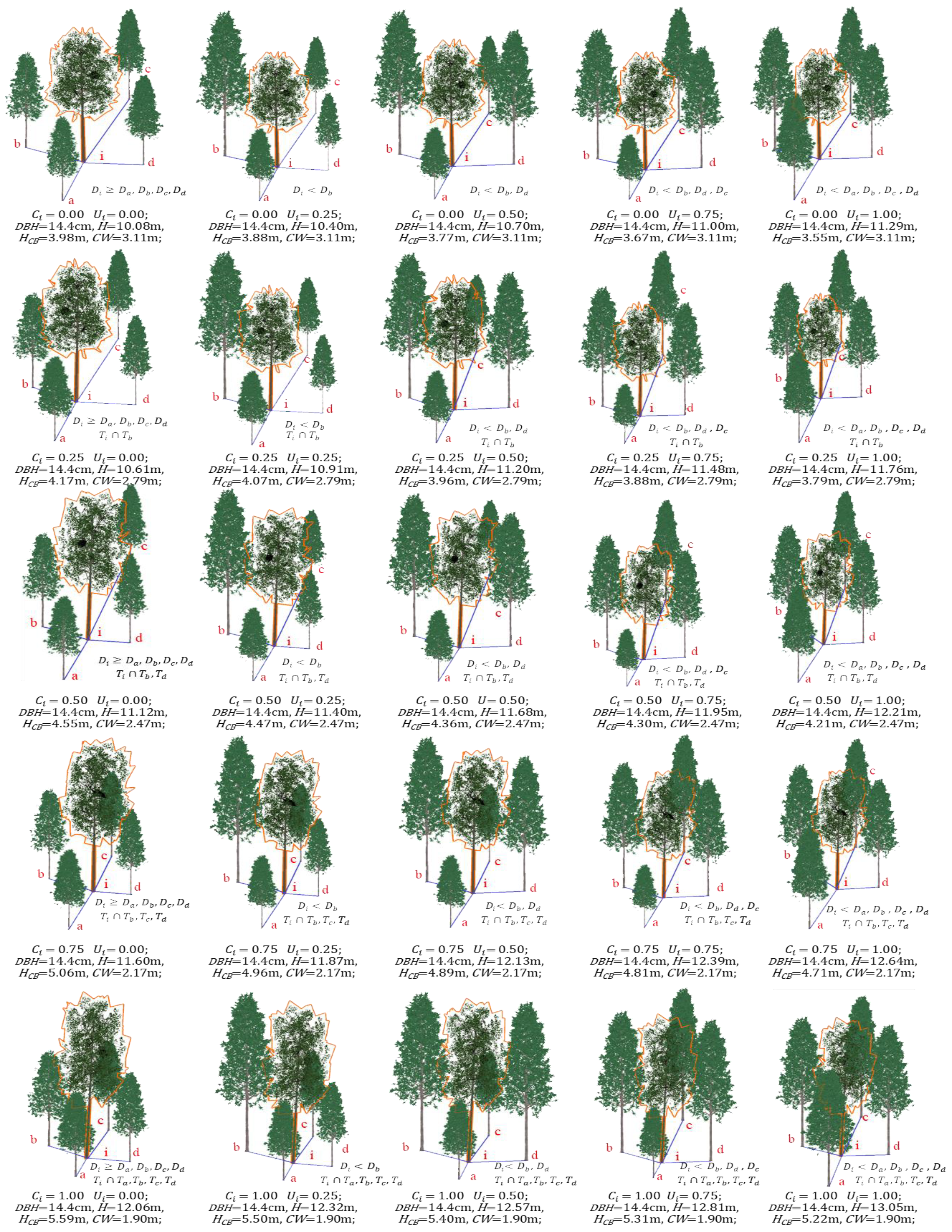
2.3.3. 3D Tree Modeling Based on a Structural Unit

Rule-based tree modeling (RTM) employs morphological parameters, such as H, H_CB, DBH, and CW, to reconstruct a reference tree i. However, ignoring the influence of spatial structure on reference tree i at a small scale would result in a decrease in the quality of 3D tree modeling and the reality of a virtual forest in forest visualization applications. Our research proposed a new method of 3D tree modeling based on a structural unit (TMSU) that incorporated structural forest theory into 3D tree modeling and achieved 3D tree modeling at the individual tree level with few parameters (see Figure 4). A nonlinear mixed-effect model was introduced in this study to improve the prediction accuracy of the morphological characteristics and parameters (e.g., H, H_CB, CW) by avoiding the random effect from the plot and increasing the applicability of the method by reducing the time and computational demand. Based on the predicted morphological data, we reconstructed a 3D tree model with our Creating Tree System (CTS) [39,40,41,42], which was developed by the Institute of Forest Resource Information Techniques of the Chinese Academy of Forestry (CAF). The CTS used in this study was based on an improved IFS algorithm [43], and it provided a graphical user interface, 3D visualization tools, and a python scripting interface, as well as the ability to create 3D tree models by selecting the tree species and inputting the H, H_CB, DBH, and CW parameters.

3. Results

3.1. Three-Dimensional Tree Morphological Model Development at the Individual Tree Level

(1) Function selection.

Table 2 displays the fit statistics of the functions. Although the evaluation indices for all the functions were nearly identical, $\mathrm{M}6\left(\mathrm{C}\mathrm{h}\mathrm{a}\mathrm{p}\mathrm{m}\mathrm{a}\mathrm{n}-\mathrm{R}\mathrm{i}\mathrm{c}\mathrm{h}\mathrm{a}\mathrm{r}\mathrm{d} \mathrm{f}\mathrm{o}\mathrm{r} \mathrm{S}\mathrm{M} \mathrm{a}\mathrm{n}\mathrm{d} \mathrm{B}\mathrm{H}\mathrm{N}’\mathrm{s} \mathrm{H}-\mathrm{D}\right)$, M5 (Power for MH’s $\mathrm{H}-D$), M17 (Walters for SM, BHN, and MH’s ${\mathrm{H}}_{\mathrm{CB}}-\mathrm{D}$), M31(Logistic for SM and BHN’s $\mathrm{C}\mathrm{W}-\mathrm{D}$), and M24 (Power for MH’s $\mathrm{C}\mathrm{W}-\mathrm{D}$) performed slightly better with the fewest parameters. As a result, these functions were chosen as the basic nonlinear model for building the morphological model.

Morphological models of the three predominant trees were the following:

$$\mathrm{SM}:H_{ij}=1.3+a\ast \left(1-exp\left(-b\ast D_{ij}\right)\right)+{\epsilon }_{ij}$$

(5)

$${H_{CB}}_{ij}=H_{ij}/(1+exp(a+b\ast D_{ij}\left)\right)+{\epsilon }_{ij}$$

(6)

$${CW}_{ij}=a/(1+b\ast exp(-c\ast D_{ij}\left)\right)+{\epsilon }_{ij}$$

(7)

$$\mathrm{BHN}:H_{ij}=1.3+a\ast (1-exp(-b\ast D_{ij}\left)\right)+{\epsilon }_{ij}$$

(8)

$${H_{CB}}_{ij}=H_{ij}/(1+exp(a+b\ast D_{ij}\left)\right)+{\epsilon }_{ij}$$

(9)

$${CW}_{ij}=a/(1+b\ast exp(-c\ast D_{ij}\left)\right)+{\epsilon }_{ij}$$

(10)

$$\mathrm{MH}:H_{ij}=1.3+a\ast {D_{ij}}^b+{\epsilon }_{ij}$$

(11)

$${H_{CB}}_{ij}=H_{ij}/(1+exp(a+(b\ast M_i+c\ast C_i+d\ast U_i)\ast D_{ij}\left)\right)+{\epsilon }_{ij}$$

(12)

$${CW}_{ij}=a\ast {D_{ij}}^b+{\epsilon }_{ij}$$

(13)

where $H_{ij},D_{ij},{H_{CB}}_{ij},{CW}_{ij}$ are the height (m), the diameter at breast height (cm), the height-to-crown base (m), and the crown width (m) of tree i in the plot j; a, b, and c are the formal parameters; and ${\epsilon }_{i\mathrm{j}}$ is an error term.

(2) Incorporating additional predictor variables.

We tested 16 different combinations of $W_i$, $M_i$, $C_i$, and $U_i$ to select the variables that made a significant contribution to the variation of the morphological characteristic ($H,H_{CB},CW$) in order to determine the influence of the spatial structure of individual trees. The statistical results showed that $C_i,M_i,\mathrm{a}\mathrm{n}\mathrm{d} U_i$ were strongly correlated with the morphological variation and, thus, were included in Equations (5)–(13). The following was the final base model used to build the morphological variation mixed-effect model:

$$\mathrm{SM}: H_{ij}=1.3+a\ast (1-exp((-b+c\ast C_i)\ast D_{ij}\left)\right)+{\mathsf{\epsilon }}_{ij}$$

(14)

$${H_{CB}}_{ij}=H_{ij}/(1+exp(a+(b+c\ast C_i)\ast D_{ij}\left)\right)+{\mathsf{\epsilon }}_{ij}$$

(15)

$${CW}_{ij}=a/(1+b\ast exp((-\mathrm{c}+\mathrm{d}\ast C_i+\mathrm{e}\ast M_i)\ast D_{ij}\left)\right)+{\mathsf{\epsilon }}_{ij}$$

(16)

$$\mathrm{BHN}:H_{ij}=1.3+a\ast (1-exp((-b+c\ast C_i+\mathrm{d}\ast U_i)\ast D_{ij}\left)\right)+{\mathsf{\epsilon }}_{ij}$$

(17)

$${H_{CB}}_{ij}=H_{ij}/(1+exp(a+(b\ast C_i+c\ast U_i)\ast D_{ij}\left)\right)+{\mathsf{\epsilon }}_{ij}$$

(18)

$${CW}_{ij}=a/(1+b\ast exp((-\mathrm{c}+\mathrm{d}\ast C_i)\ast D_{ij}\left)\right)+{\mathsf{\epsilon }}_{ij}$$

(19)

$$\mathrm{MH}:H_{ij}=1.3+(a+c\ast M_i+\mathrm{d}\ast C_i)\ast {D_{ij}}^b+{\mathsf{\epsilon }}_{ij}$$

(20)

$${H_{CB}}_{ij}=H_{ij}/(1+exp(a+(b\ast M_i+c\ast C_i+d\ast U_i)\ast D_{ij}\left)\right)+{\mathsf{\epsilon }}_{ij}$$

(21)

$${CW}_{ij}=(a+c\ast C_i+d\ast M_i)\ast {D_{ij}}^b+{\mathsf{\epsilon }}_{ij}$$

(22)

where $H_{ij},D_{ij},{H_{CB}}_{ij},{CW}_{ij}$ are the height (m), the diameter at breast height (cm), the height-to-crown base (m), and the crown width (m) of tree i in the plot j; a, b, and c are the formal parameters; $C_i,$ $M_i,$ and $U_i$ are the degree of crowding, mingling, and dominance of the reference tree i base on structural unit; and ${\epsilon }_{ij}$ is an error term.

(3) Constructing mixed-effect model with parameters for the spatial structure.

After considering the model parameters (a, b, c, d, e) involved, there were seven different combinations of random effects at the sample plot level for Equations (14), (15) and (18), 15 different combinations for Equations (17), (19) and (20)–(22), and 31 different combinations for Equation (16). When fitted to the data, only model alternatives 5, 6, and 10 converged in Equations (14)–(16), respectively; whereas 12, 6, and 1 converged in Equations (17)–(19), respectively. Model alternatives 5, 9, and 6 converged in Equations (20)–(22), respectively. Among the models that converged, the NLME model with random parameters on a/b/c in Equation (14), c in Equation (15), a/b in Equation (16), b/c in Equation (17), b/c in Equation (18), a/b/d in Equation (19), a in Equation (20), a in Equation (21), and c/d in Equation (22) showed the smallest AIC and BIC. Three dominant trees’ morphological models with mixed effects became the following:

$$\mathrm{SM}:H_{ij}=1.3+({\beta }_1+u_{1j})\ast (1-exp((-{\beta }_2-u_{2j}+({\beta }_3+u_{3j})\ast C_i)\ast D_{ij}\left)\right)+{\mathsf{\epsilon }}_{ij}$$

(23)

$${H_{CB}}_{ij}=H_{ij}/(1+exp({\beta }_1+({\beta }_2+({\beta }_3+u_{1j})\ast C_i)\ast D_{ij}\left)\right)+{\mathsf{\epsilon }}_{ij}$$

(24)

$${CW}_{ij}=({\beta }_1+u_{1j})/(1+({\beta }_2+u_{2j})\ast exp((-{\beta }_3+{\beta }_4\ast C_i+{\beta }_5\ast M_i)\ast D_{ij}\left)\right)+{\mathsf{\epsilon }}_{ij}$$

(25)

$$\mathrm{BHN}:H_{ij}=1.3+{\beta }_1\ast (1-exp((-{\beta }_2-u_{1j}+({\beta }_3+u_{2j})\ast C_i+{\beta }_4\ast U_i)\ast D_{ij}\left)\right)+{\mathsf{\epsilon }}_{ij}$$

(26)

$${H_{CB}}_{ij}=H_{ij}/(1+exp({\beta }_1+({\beta }_2+u_{1j})\ast C_i+{(\beta }_3+u_{2j})\ast U_i)\ast D_{ij}\left)\right)+{\mathsf{\epsilon }}_{ij}$$

(27)

$${CW}_{ij}=({\beta }_1+u_{1j})/(1+({\beta }_2+u_{2j})\ast exp((-{\beta }_3+({\beta }_4+u_{3j})\ast C_i)\ast D_{ij}\left)\right)+{\mathsf{\epsilon }}_{ij}$$

(28)

$$\mathrm{MH}: H_{ij}=1.3+({\beta }_1+u_{1j}+{\beta }_3\ast M_i+{\beta }_4\ast C_i)\ast {D_{ij}}^{{\beta }_2}+{\mathsf{\epsilon }}_{ij}$$

(29)

$${H_{CB}}_{ij}=H_{ij}/(1+exp({\beta }_1+u_{1j}+({\beta }_2\ast M_i+{\beta }_3\ast C_i+{\beta }_4\ast U_i)\ast D_{ij}\left)\right)+{\mathsf{\epsilon }}_{ij}$$

(30)

$${CW}_{ij}=({\beta }_1+({\beta }_3+u_{1j})\ast C_i+({\beta }_4+u_{2j})\ast M_i)\ast {D_{ij}}^{{\beta }_2}+{\mathsf{\epsilon }}_{ij}$$

(31)

where ${\beta }_1-{\beta }_5$ are mixed-effect parameters; $u_{1j},u_{2j},u_{3j},{\mathrm{a}\mathrm{n}\mathrm{d} u}_{4j}$ are random-effect parameters generated by the plot on ${\beta }_1,{\beta }_2,{\beta }_3,{\beta }_4$, respectively; and ${\epsilon }_{ij}$ is an error term.

(4) Within-plot variance–covariance (R) structure.

Because our data did not show spatial autocorrelations, we assumed the matrix of the within-plot error autocorrelation was an identity matrix. However, we found heteroscedasticity in our preliminary analysis even after the random effects were included in the morphological model with SSP. We then evaluated three variance functions for their heteroscedasticity-reducing performances. The results showed that Equations (24), (27)–(30) and (31) produced significantly different results than the models without variance functions, whereas Equations (23), (25) and (26) did not. According to the AIC and Loglik values, the power variance function and constant power variance function performed the best among the tested variance functions (

Table 3. Performance of mixed-effect model Equations (23)–(31) using morphological data with different variance functions. SM, BHN, and MH represent Cunninghamia lanceolata, Machilus pauhoi, and Schima superba, respectively.

Species	Model	Evaluation Indices	Residual Variance Function
			Null	Exponential Function	Power Function	Constant Plus Power Function
SM	Equation (23)	AIC	4336.224	4337.334	4337.458	4339.477
		Loglik	−2158.11	−2157.667	−2157.729	−2157.739
		p Value		p > 0.05	p > 0.05	p > 0.05
	Equation (24)	AIC	3438.982	3421.818	3421.136	3423.136
		Loglik	−1712.491	−1702.909	−1702.568	−1702.568
		p Value		p < 0.0001	p < 0.0001	p < 0.0001
	Equation (25)	AIC	1935.082	1935.461	1934.881	1936.881
		Loglik	−960.5411	−959.7304	−959.441	−959.4404
		p Value		p > 0.05	p > 0.05	p > 0.05
BHN	Equation (26)	AIC	3825.354	3827.209	3825.14	3827.14
		Loglik	−1906.677	−1906.604	−1905.57	−1905.57
		p Value		p > 0.05	p > 0.05	p > 0.05
	Equation (27)	AIC	3322.544	3249.631	3231.132	3235.042
		Loglik	−1906.677	−1616.815	−1607.57	−1608.521
		p Value		p < 0.0001	p < 0.0001	p < 0.0001
	Equation (28)	AIC	3160.599	2365.384	2449.84	2342.501
		Loglik	−1574.299	−1175.692	−1217.92	−1163.251
		p Value	p < 0.0001	p < 0.0001	p < 0.0001	p < 0.0001
MH	Equation (29)	AIC	4316.121	4313.26	4310.291	4312.291
		Loglik	−2150.061	−2147.63	−2146.145	−2146.145
		p Value		p < 0.05	p < 0.05	p < 0.05
	Equation (30)	AIC	3798.104	3701.172	3699.936	3701.532
		Loglik	−1888.052	−1838.586	−1837.968	−1837.766
		p Value		p < 0.0001	p < 0.0001	p < 0.0001
	Equation (31)	AIC	2462.686	2418.486	2427.477	2416.827
		Loglik	−1223.343	−1200.243	−1204.739	−1198.413
		p Value		p < 0.0001	p < 0.0001	p < 0.0001

). Therefore, the final modes were the following: Equation (23) + null, Equation (24) + power function, Equation (25) + power function, Equation (26) + power function, Equation (27) + power function, Equation (28) + constant plus power function, Equation (29) + power function, Equation (30) + power function, and Equation (31) + constant plus power function. By including the variance function, the model’s AIC decreased from 3438.982 to 3421.136 in Equation (24), from 1935.082 to 1934.881 in Equation (25), from 3825.354 to 1934.881 in Equation (26), from 3322.544 to 3231.132 in Equation (27), from 3160.599 to 2342.501 in Equation (28), from 4316.121 to 4310.291 in Equation (29), from 3798.104 to 3699.936 in Equation (30), and from 2462.686 to 2416.827 in Equation (31).

(5) Estimation of parameters.

All parameter estimates of the OLS and NLME models at the sample plot level with the power variance function or constant plus power variance function were significantly different from zero (p < 0.05), and the parameters are listed in

Table 4. Parameter estimates and evaluation indices of each model. SM, BHN, and MH represent Cunninghamia lanceolata, Machilus pauhoi, and Schima superba, respectively. If the letters a, b, and c, are the same, it represents no significant difference between models; otherwise, there are significant differences between models. ** and *** represent significant and extremely significant, respectively.

Species	Formula	Model	Fixed Parameters					Evaluation Indexes
			𝛽1	𝛽2	𝛽3	𝛽4	𝛽5	AIC	Loglik	p Value
SM	H-D	Equation (5)	33.4665	0.0266	——	——	——	4686.538	−2340.27	a
		Equation (14)	32.5791	0.0252	−0.0037	——	——	4350.543	−2168.27	b ***
		Equation (23)	36.7543	0.0236	−0.0045	——	——	4336.224	−2158.11	c ***
	HCB-H	Equation (6)	0.4501	−0.0012	——	——	——	3488.336	−1741.17	a
		Equation (15)	0.4230	0.0061	−0.0087	——	——	3441.651	−1716.83	b ***
		Equation (24)	0.3896	0.0073	−0.0096	——	——	3421.136	−1702.57	c **
	CW-D	Equation (7)	5.9591	2.4952	0.0538	——	——	2224.718	−1108.36	a
		Equation (16)	5.5826	2.3971	0.0461	−0.0367	0.0153	2030.871	−1009.44	b ***
		Equation (25)	5.5212	2.4130	0.0520	−0.0310	0.0162	1934.881	−959.441	c ***
BHN	H-D	Equation (8)	19.3411	0.0540	——	——	——	3970.13	−1982.07	a
		Equation (17)	19.6529	0.0399	−0.0123	−0.0072	——	3935.849	−1962.93	b ***
		Equation (26)	20.0990	0.0399	−0.0133	−0.0078	——	3825.14	−1905.57	c ***
	HCB-H	Equation (9)	0.2933	0.0043	——	——	——	3404.81	−1699.41	a
		Equation (18)	0.0384	−0.0310	0.0202	——	——	3335.732	−1663.87	b ***
		Equation (27)	0.0408	−0.0308	0.0133	——	——	3231.132	−1607.57	c ***
	CW-D	Equation (10)	8.3246	4.1547	0.0885	——	——	3218.003	−1605	a
		Equation (19)	8.4723	3.7601	0.0501	−0.0386	——	3188.058	−1589.03	b ***
		Equation (28)	6.7421	3.2953	0.0721	−0.0455	——	2342.501	−1163.25	c ***
MH	H-D	Equation (11)	2.5166	0.5378	——	——	——	4577.814	−2285.91	a
		Equation (20)	2.6616	0.5135	−0.3857	0.3370	——	4526.287	−2258.14	b ***
		Equation (29)	2.3741	0.5686	−0.2014	0.0622	——	4310.291	−2146.15	c ***
	HCB-H	Equation (12)	0.8568	−0.0036	——	——	——	3980.823	−1987.41	a
		Equation (21)	0.5636	0.0253	0.0185	−0.0103	——	3919.156	−1954.58	b ***
		Equation (30)	0.5479	0.0277	0.0132	−0.0026	——	3699.936	−1837.97	c ***
	CW-D	Equation (13)	0.8478	0.5819	——	——	——	2749.965	−1371.98	a
		Equation (22)	0.5918	0.5606	0.3178	0.1041	——	2554.176	−1272.09	b ***
		Equation (31)	0.6514	0.5591	0.2820	0.0519	——	2416.827	−1198.41	c ***

. When the fixed parameters were substituted into Equations (23)–(31), the morphological model for SM, BHN, and MH, respectively, became the following:

$$\mathrm{SM}:H_{ij}=1.3+(36.7543+u_{1j})\ast (1-exp((-0.0236-u_{2j}+(-0.0045+u_{3j})\ast C_i)\ast D_{ij}\left)\right)+{\mathsf{\epsilon }}_{ij}$$

(32)

$${H_{CB}}_{ij}=H_{ij}/(1+exp(0.3896+(0.0073+(-0.0096+u_{1j})\ast C_i)\ast D_{ij}\left)\right)+{\mathsf{\epsilon }}_{ij}$$

(33)

$${CW}_{ij}=(5.5212+u_{1j})/(1+(2.4130+u_{2j})\ast exp((-0.0520+(-0.0310\ast C_i)+0.0162\ast M_i)\ast D_{ij}\left)\right)+{\mathsf{\epsilon }}_{ij}$$

(34)

$$\mathrm{BHN}: H_{ij}=1.3+20.0990\ast (1-\mathrm{e}\mathrm{x}\mathrm{p}((-0.0399-u_{1j}+(-0.0133+u_{2j})\ast C_i+(-0.0078\ast U_i\left)\right)\ast D_{ij}\left)\right)+{\mathsf{\epsilon }}_{ij}$$

(35)

$${H_{CB}}_{ij}=H_{ij}/(1+exp(0.0408+(-0.0308+u_{1j})\ast C_i+(0.0133+u_{2j})\ast U_i)\ast D_{ij}))+{\mathsf{\epsilon }}_{ij}$$

(36)

$${CW}_{ij}=(6.7421+u_{1j})/(1+(3.2953+u_{2j})\ast exp((-0.0721+(-0.0455+u_{3j})\ast C_i)\ast D_{ij}\left)\right)+{\mathsf{\epsilon }}_{ij}$$

(37)

$$\mathrm{MH}:H_{ij}=1.3+(2.3741+u_{1j}-0.2014\ast M_i+0.0622\ast C_i)\ast {D_{ij}}^{0.5686}+{\mathsf{\epsilon }}_{ij}$$

(38)

$${H_{CB}}_{ij}=H_{ij}/(1+exp(0.5479+u_{1j}+(0.0277\ast M_i+0.0132\ast C_i-0.0026\ast U_i)\ast D_{ij}\left)\right)+{\mathsf{\epsilon }}_{ij}$$

(39)

$${CW}_{ij}=(0.6514+(0.2820+u_{1j})\ast C_i+(0.0519+u_{2j})\ast M_i)\ast {D_{ij}}^{0.5591}+{\mathsf{\epsilon }}_{ij}$$

(40)

In order to validate the effect of the plot level and SSP on the model parameters, we recorded the performance statistics and parameters of the final NLME and OLS models. According to the AIC, Loglik, and p-value in Table 4, As shown, Equations (23)–(31) had the smallest AIC and the largest Loglik values, and there was a significant difference between Equations (5) and (14); Equations (14) and (23); Equations (6) and (15); Equations (15) and (24); Equations (7) and (16); Equations (16) and (25); Equations (8) and (17); Equations (17) and (26); Equations (9) and (18); Equations (18) and (27); Equations (10) and (19); Equations (19) and (28); Equations (11) and (20); Equations (20) and (29); Equations (12) and (21); Equations (21) and (30); Equations (13) and (22); and, finally, between Equations (22) and (31), which indicated that the plot and SSP had significant effects on the morphological models of SM, BHN, and MH.

(6) Assessment and analysis of morphological models.

Most models of the morphological characteristics in TMSU differed significantly from the models in RTM, according to

Table 5. Parameter estimates and evaluation indices of each model. SM, BHN, and MH represent Cunninghamia lanceolata, Machilus pauhoi, and Schima superba, respectively; $u_{1j}$, $u_{2j}$,$u_{3j}$ are the random effect parameters caused by the jth sample plot on 𝛽_1, 𝛽_2, 𝛽₃, respectively.

Species	Formula	Model	Variance Components						Fit Statistics
			${\mathsf{\sigma }}_{{\mathit{u}}_{1\mathit{j}}}^2$	${\mathsf{\sigma }}_{{\mathit{u}}_{2\mathit{j}}}^2$	${\mathsf{\sigma }}_{{\mathit{u}}_{3\mathit{j}}}^2$	${\mathsf{\sigma }}_{{\mathit{u}}_{1\mathit{j}}}{\mathit{\sigma }}_{{\mathit{u}}_{2\mathit{j}}}$	${\mathsf{\sigma }}_{{\mathit{u}}_{1\mathit{j}}}{\mathit{\sigma }}_{{\mathit{u}}_{3\mathit{j}}}$	${\mathsf{\sigma }}_{{\mathit{u}}_{2\mathit{j}}}{\mathit{\sigma }}_{{\mathit{u}}_{3\mathit{j}}}$	R2	E	RMSE
SM	H-D	Equation (5)	——	——	——	——	——	——	0.7155	−0.0201	2.7644
		Equation (14)	——	——	——	——	——	——	0.7369	−0.0199	2.6584
		Equation (23)	4.99 × 100	7.51 × 10−5	2.90 × 10−5	−9.86 × 10−1	8.83 × 10−1	−9.47 × 10−1	0.8203	−0.0190	2.1971
	HCB-H	Equation (6)	——	——	——	——	——	——	0.6121	0.0635	1.4820
		Equation (15)	——	——	——	——	——	——	0.6313	0.0739	1.4450
		Equation (24)	3.78 × 10−6	——	——	——	——	——	0.6406	0.0670	1.4265
	CW-D	Equation (7)	——	——	——	——	——	——	0.4276	−0.0004	0.7671
		Equation (16)	——	——	——	——	——	——	0.5341	−0.0004	0.6921
		Equation (25)	1.24 × 10−1	2.95 × 10−2	——	−1.81 × 10−1	——	——	0.5965	−0.0013	0.6441
BHN	H-D	Equation (8)	——	——	——	——	——	——	0.6752	0.0250	2.1741
		Equation (17)	——	——	——	——	——	——	0.6887	0.0201	2.1285
		Equation (26)	3.17 × 10−6	9.95 × 10−5	——	−8.83 × 10−1	——	——	0.7376	0.0205	1.9542
	HCB-H	Equation (9)	——	——	——	——	——	——	0.4095	0.0482	1.5897
		Equation (18)	——	——	——	——	——	——	0.4542	0.0383	1.5284
		Equation (27)	2.49 × 10−5	1.61 × 10−4	——	−4.30 × 10−1	——	——	0.4860	0.0467	1.4832
	CW-D	Equation (10)	——	——	——	——	——	——	0.4594	−0.0012	1.4319
		Equation (19)	——	——	——	——	——	——	0.4782	−0.0015	1.4068
		Equation (28)	3.59 × 100	3.41 × 100	3.47 × 10−13	1.00 × 100	−3.20 × 10−2	−3.20 × 10−2	0.5271	0.0032	1.3393
MH	H-D	Equation (11)	——	——	——	——	——	——	0.5161	0.0008	2.4594
		Equation (20)	——	——	——	——	——	——	0.5426	−0.0021	2.3912
		Equation (29)	7.43 × 10−2	——	——	——	——	——	0.6473	−0.0029	2.0999
	HCB-H	Equation (12)	——	——	——	——	——	——	0.3018	−0.0148	1.8170
		Equation (21)	——	——	——	——	——	——	0.3468	−0.0177	1.7575
		Equation (30)	3.77 × 10−2	——	——	——	——	——	0.4282	0.0078	1.6443
	CW-D	Equation (13)	——	——	——	——	——	——	0.5322	0.0020	0.9734
		Equation (22)	——	——	——	——	——	——	0.6180	0.0054	0.8796
		Equation (31)	1.10 × 10−2	2.76 × 10−3	——	−9.95 × 10−1	——	——	0.6658	0.0077	0.8228

. For example, as compared to the morphological models of Equations (5)–(13) and (23)–(31), which were based on NLME and incorporated variables of the spatial structurers, we were able to significantly increase the prediction accuracy of the morphological characteristics by 10.4%, 3.02%, and 17.8% for SM’s H, HCB, and CW, respectively; 6.5%, 7.6%, and 8.9% for BHN’s H, HCB, and CW, respectively; and 13.3%, 15.7%, and 13.4% for MH’s H, HCB, and CW, respectively.

A box plot of the residuals of the dependent variable classes of three dominant trees was examined to further assess the feasibility of the fitted models based on OLS and NLME (see Figure 5). In each plot, nearly all absolute values of the standard residuals based on OLS and NLME models were less than two. Furthermore, the residuals from the NLME model showed no significant trends, whereas some residual plots from the OLS model did, such as the HCB model of Cunninghamia lanceolata, Machilus pauhoi, and Schima superba, as well as the CW model of Machilus pauhoi and Schima superba. Only a few larger deviations were observed for trees that were unusually large or small. The residual from the NLME model exhibited no variance in heteroskedasticity. As a result, the NLME models Equations (32)–(40) had superior statistical performance and could be used for SM, BHN, and MH’s 3D tree modeling in TMSU, respectively.

3.2. Analysis of 3D Tree Modeling Based on a Structural Unit

We discovered that the reference tree’s $C_i,M_i,\mathrm{a}\mathrm{n}\mathrm{d} U_i$ had a substantial influence on the morphological features of morphological characteristic of SM, BHN, and MH, according to the analytical results of the nonlinear mixed-effect morphological models of three dominant species. For example, (i) crowding and mingling had a significant impact on SM’s morphological characteristics: the higher the degree of crowding, the higher the tree height and the height-to-crown base, the smaller the crown width, while under the same crowding, the higher the mingling, the bigger the crown width. (ii) Crowding and dominance had an impact on BHN’s morphological characteristics: the bigger the crowding, the higher the tree height and the height-to-crown base, the smaller the crown width, while under the same crowding, the higher the dominance, the bigger the tree height and the lower the height-to-crown base. (iii) Crowding, dominance, and mingling all had an impact on the morphological characteristics of MH: the bigger the crowding, the higher the tree height and the smaller the crown width, while under the same crowding and mingling, the higher the dominance, the higher the height-to-crown base. (see Figure 6).

In this study, we have selected three very different scenes for SM, BHN, and MH as examples to reconstruct 3D tree modeling with a structural unit (see Figure 7). Based on the value classes of $C_i,M_i,\mathrm{a}\mathrm{n}\mathrm{d} U_i$, we constructed the SM and BHN model libraries with 25 scenes each (see Appendix A Figure A1 and Figure A2) and an MH model library with 125.

4. Discussion

4.1. The Development of Morphological Characteristic Models Involving Forest Spatial Structure in TMSU

A model of morphological characteristics involving forest spatial structure is an essential component of 3D tree modeling based on a structural unit. By acquiring several morphological parameters for 3D tree reconstruction, such as tree height, height-to-crown base, diameter at breast height, and crown width, RTM used fewer micro-characteristics of the individual trees [4,5,6,7]. However, forest environments are not homogeneous even at very small scales. The spatial structures must be incorporated into the morphological characteristics in order to accurately model 3D trees in an environment with a high degree of structural diversity and heterogeneity [12,13,14]. In our study, TMSU used four spatial-structure variables (e.g., $W_i$, $M_i$, $C_i$, and $U_i$) to describe the spatial structures and their effects on morphological traits. According to Table 4, we discovered that these spatial structures could increase the precision with which morphological characteristics were predicted due to the spatial heterogeneity of a reference tree. For example, as compared to the RTM model Equations (5)–(13), the TMSU model Equations (14)–(22) incorporated variables of the spatial structures and then improved its prediction accuracy of the morphological characteristics by 2.1%, 1.9%, and 10.7% for SM’s H, H_CB, and CW, respectively; 1.4%, 4.5%, and 1.9% for BHN’s H, H_CB, and CW, respectively; and finally, 2.7%, 4.5%, and 8.9% for MH’s H, H_CB, and CW, respectively. However, when developing morphological characteristic models, researchers have suggested that adding excessive parameters affected model convergence and lengthened the time to compute parameter estimates, especially for the nonlinear mixed-effect modeling strategy used in this study [27,28,44]. Furthermore, adding a number of tree or spatial-structure variables to the inventory increased the cost and time required to obtain the measurements for those variables [29,44]. Therefore, for the final morphological prediction model of SM in TMSU, we selected one tree variable (D) and two spatial-structure variables ($C_i$, $M_i$); one tree variable (D) and two spatial-structure variables ($C_i$, $U_i$) for the final morphological prediction model of BHN; and one tree variable (D) and three spatial-structure variables ($C_i$, $U_i$, $M_i$) for the final morphological prediction model of MH.

Nonlinear mixed-effect models are appealing for the analysis of hierarchically structured data that are auto-correlated, as compared to the OLS model because of their flexibility in accounting for the covariate structure that is overlooked in conventional regression procedures. Therefore, in this study, we selected the Chapman–Richards, Walters, logistic, and power models as the base morphological models based on the statistical variables ${\mathrm{R}}^2$, E, and RMSE, and then we integrated them with a nonlinear mixed-effect model approach at the plot level to construct morphological models of three dominant trees involving spatial-structure parameters. As shown in Table 5, a random effect model in TMSU Equations (23)–(31) outperformed a model without a random effect in RTM Equations (14)–(22) in terms of prediction accuracy for the full dataset. The result was consistent with most research conclusions [24,25,26,27,28]. As a result, morphological models of three dominant trees in TMSU were chosen for 3D tree modeling due to their higher precision and spatial capabilities. In addition, the morphological models in TMSU were limited in their capacity to handle changes in spatial structures (e.g., those caused by human activity or natural succession) [45] and complete data acquisition that could reflect different spatial-structure conditions. Generally, as the spatial structure of the planted mixed forest would not be significantly altered in a short time, the models in TMSU could be utilized for producing a short-term forecast (less than 5 years). Therefore, in order to improve the applicability of the morphological model in TMSU, we will consider climate variables, in addition to natural succession and human activities, and devise more plots with different spatial-structure conditions in our next project [46,47].

4.2. Three-Dimensional Tree Modeling in a Highly Heterogeneous Forest Environment

In forest visualization research, accurate 3D tree modeling with heterogeneous spatial forest structures is required (e.g., forest quality assessment, health supervision, and forest management planning and assessment) [48]. Given the complexity of forest structures and heterogeneous habitats, describing the relationship between any individual tree and its neighbors in a 3D tree model is a significant issue. In this study, we addressed the challenges of 3D tree modeling in a complex and highly heterogeneous forest environment in order to determine the spatial-structure variables, explore the relationships between spatial structures and morphological characteristics, and achieve 3D tree modeling based on a structural unit.

Most researchers have developed various qualitative and quantitative indices to describe the reference tree and its neighbor trees in a forest stand, such as the index of Clark and Evans [49], the diffusion index [50], Ripley’s K-function [51], the K-function [52], the O-ring statistic [53], the Gini coefficient [54], Pielou’s isolation index [55], the mean directional index [56], Gadow’s species mingling [57], the mixed ratio [58], and the uniform angle index [59,60]. However, some of these indices have been predominantly used in forestry and ecology, and they do not meet the prerequisites for visually and intuitively portraying 3D tree modeling based on a structural unit [19,20]. In addition, certain approaches for analyzing spatial structures consider the neighboring tree species to some extent, although they can only describe the overall or unilateral structure of the reference tree population. For example, the size differentiation, mixed conditions, and the degree of crowding of the reference tree at different distance scales remained unknown when using $W_i$ to analyze the distribution patterns. Therefore, these methods solely considered the distribution pattern and overlooked factors such as the tree size, the degree of crowding, and the degree of species aggregation. Furthermore, an entirely different structure could yield the same outcome. Obviously, it has been challenging to accurately depict the spatial structure of a tree population. The forest is a complex and dynamic ecosystem, particularly when it contains many different species and has a highly heterogeneous spatial structure. The four most significant characteristics of the population structure for any species in a mixed forest may be interspecific and intraspecific variances in tree sizes, species mingling, crowding, and distribution patterns [60]. The spatial structural parameters ${W_i,M}_i,C_i,\mathrm{a}\mathrm{n}\mathrm{d} U_i$ were used in TMSU to describe the relationships between any reference tree and its four adjacent neighboring trees. It uncovered reference tree population characteristics and modeled a 3D tree in a more accurate and thorough manner by simultaneously employing two or more pieces of structural information.

According to TMSU-based morphological models, we found that $C_i,M_i,{\mathrm{a}\mathrm{n}\mathrm{d} U}_i$ had a strong influence on the morphological characteristic of SM, BHN, and MH. For example, in SM, BHN, and MH, there was an identical phenomenon where the degree of crowding had a positive relationship with tree height, height-to-crown base, and crown width, which could be related to a growth response strategy of trees in a crowded and highly competitive environment to increase the tree’s height to occupy the main layer of the forest and obtain more resources, such as light, moisture, and nutrition [17,60]. This could also promote the self-thinning of the branches, which increases the height-to-crown base for the limited availability of the light resource [10], as well as retaining a narrow crown width due to competition with conspecific and nonspecific species [16]. Furthermore, under the same degree of crowding, mingling was positively correlated with tree crown width in SM, and dominance was positively correlated with tree height but negatively correlated with the height-to-crown base in BHN; under the same crowding and mingling conditions, the dominance was positively correlated with the height-to-crown base in MH. The results could be linked to the competitive response mechanism of various tree species, such as light transmittance, shade tolerance, and biological characteristics. Therefore, considering the unique coupling responses between the spatial-structure parameters and the morphological characteristics, we created model libraries for the three dominant species with 25 scenes based on the value classes of $C_i \mathrm{a}\mathrm{n}\mathrm{d} M_i$ for SM; 25 scenes based on the value classes of $C_i \mathrm{a}\mathrm{n}\mathrm{d} U_i$ for BHN; and 125 scenes based on the value classes of $C_i,M_i,\mathrm{a}\mathrm{n}\mathrm{d} U_i$ for MH, respectively.

5. Conclusions

This study provided a new approach for 3D tree modeling TMSU. The differences between RTM and TMSU were focused on: (i) Four spatial structural parameters ($W_i$, $M_i$, $C_i$, and $U_i$) were incorporated into the morphological characteristic models of the reference trees and revealed the relationship between the spatial-structure variables and the morphological features. (ii) The nonlinear mixed-effect model was introduced into the parameter estimation of the TMSU-based morphological model for higher precision and applicability. By comparing the two approaches, RTM and TMSU, we found that (i) the prediction accuracy of the TMSU-based morphological model increased by 10.4%, 3.02%, and 17.8% for SM’s H, HCB, and CW, respectively; 6.5%, 7.6%, and 8.9% for BHN’s H, HCB, and CW, respectively; and 13.3%, 15.7%, and 13.4% for MH’s H, HCB, and CW, respectively, as compared to the RTM morphological models. (ii) TMSU provided more spatial-structure information with fewer parameters in the morphological models and revealed the relationships between the spatial structures and the morphological traits of the reference tree.

References

1. Paulus, S.; Dupuis, J.; Mahlein, A.K.; Kuhlmann, H. Surface feature based classification of plant organs from 3D laserscanned point clouds for plant phenotyping. BMC Bioinform. 2013, 14, 238. [Google Scholar] [CrossRef] [Green Version]
2. Thapa, S.; Zhu, F.; Walia, H.; Yu, H.; Ge, Y. A novel LiDAR-based instrument for high-throughput, 3D measurement of morphological traits in maize and sorghum. Sensors 2018, 18, 1187. [Google Scholar] [CrossRef] [Green Version]
3. Indirabai, I.; Nair, M.V.H.; Jaishanker, R.N.; Nidamanuri, R.R. Terrestrial laser scanner based 3D reconstruction of trees and retrieval of leaf area index in a forest environment. Ecol. Inform. 2019, 53, 100986. [Google Scholar] [CrossRef]
4. Sun, R.; Jia, J.; Jaeger, M. Intelligent tree modeling based on L-system. In Proceedings of the 2009 IEEE 10th International Conference on Computer-Aided Industrial Design & Conceptual Design, Wenzhou, China, 26–29 November 2009; pp. 1096–1100. [Google Scholar] [CrossRef]
5. Wang, G.; Zhang, D.; Zhou, K.; Jia, J. Rule and reuse based lightweight modeling and real time web3D rendering of forest scenes. In Proceedings of the 23rd International ACM Conference on 3D Web Technology, Poznań, Poland, 20–22 June 2018; pp. 1–8. [Google Scholar] [CrossRef]
6. Tang, L.; Peng, X.; Chen, C.; Huang, H.; Lin, D. Three-dimensional Forest growth simulation in virtual geographic environments. Earth Sci. Inform. 2019, 12, 31–41. [Google Scholar] [CrossRef]
7. Kim, D.; Kang, W.H.; Hwang, I.; Kim, J.; Kim, J.H.; Park, K.S.; Son, J.E. Use of structurally-accurate 3D plant models for estimating light interception and photosynthesis of sweet pepper (Capsicum annuum) plants. Comput. Electron. Agric. 2020, 177, 105689. [Google Scholar] [CrossRef]
8. Zhang, X.; Li, H.; Dai, M.; Ma, W.; Quan, L. Data-driven synthetic modeling of trees. IEEE Trans. Vis. Comput. Graph. 2014, 20, 1214–1226. [Google Scholar] [CrossRef]
9. Seidel, D.; Hoffmann, N.; Ehbrecht, M.; Juchheim, J.; Ammer, C. How neighborhood affects tree diameter increment–new insights from terrestrial laser scanning and some methodical considerations. For. Ecol. Manag. 2015, 336, 119–128. [Google Scholar] [CrossRef]
10. Bayer, D.; Seifert, S.; Pretzsch, H. Structural crown properties of Norway spruce (Picea abies [L.] Karst.) and European beech (Fagus sylvatica [L.]) in mixed versus pure stands revealed by terrestrial laser scanning. Trees 2013, 27, 1035–1047. [Google Scholar] [CrossRef]
11. Seidel, D.; Leuschner, C.; Müller, A.; Krause, B. Crown plasticity in mixed forests—Quantifying asymmetry as a measure of competition using terrestrial laser scanning. For. Ecol. Manag. 2011, 261, 2123–2132. [Google Scholar] [CrossRef]
12. Forrester, D.I.; Benneter, A.; Bouriaud, O.; Bauhus, J. Diversity and competition influence tree allometric relationships–developing functions for mixed-species forests. J. Ecol. 2017, 105, 761–774. [Google Scholar] [CrossRef] [Green Version]
13. Vincent, G.; Harja, D. Exploring ecological significance of tree crown plasticity through three-dimensional modelling. Ann. Bot. 2008, 101, 1221–1231. [Google Scholar] [CrossRef] [Green Version]
14. Purves, D.W.; Lichstein, J.W.; Pacala, S.W. Crown plasticity and competition for canopy space: A new spatially implicit model parameterized for 250 North American tree species. PLoS ONE 2007, 2, e870. [Google Scholar] [CrossRef]
15. Valladares, F.; Niinemets, Ü. Shade tolerance, a key plant feature of complex nature and consequences. Annu. Rev. Ecol. Evol. Syst. 2008, 39, 237–257. [Google Scholar] [CrossRef] [Green Version]
16. Jucker, T.; Bouriaud, O.; Coomes, D.A. Crown plasticity enables trees to optimize canopy packing in mixed-species forests. Funct. Ecol. 2015, 29, 1078–1086. [Google Scholar] [CrossRef] [Green Version]
17. Lines, E.R.; Zavala, M.A.; Purves, D.W.; Coomes, D.A. Predictable changes in aboveground allometry of trees along gradients of temperature, aridity and competition. Glob. Ecol. Biogeogr. 2012, 21, 1017–1028. [Google Scholar] [CrossRef]
18. Grueters, U.; Seltmann, T.; Schmidt, H.; Horn, H.; Pranchai, A.; Vovides, A.G.; Peters, R.; Vogt, J.; Dahdouh-Guebas, F.; Berger, U. The mangrove forest dynamics model mesoFON. Ecol. Model. 2014, 291, 28–41. [Google Scholar] [CrossRef]
19. Pommerening, A.; Gaulton, R.; Magdon, P.; Myllymäki, M. CanopyShotNoise–An individual-based tree canopy modelling framework for projecting remote-sensing data and ecological sensitivity analysis. Int. J. Remote Sens. 2021, 42, 6837–6865. [Google Scholar] [CrossRef]
20. Fischer, F.J.; Labriere, N.; Vincent, G.; Hérault, B.; Alonso, A.; Memiaghe, H.; Bissiengou, P.; Kenfack, D.; Saatchi, S.; Chaveet, J. A simulation method to infer tree allometry and forest structure from airborne laser scanning and forest inventories. Remote Sens. Environ. 2020, 251, 112056. [Google Scholar] [CrossRef]
21. Yang, Z.; Liu, Q.; Luo, P.; Ye, Q.; Sharma, R.P.; Duan, G.; Zhang, H.; Fu, L. Nonlinear mixed-effects height to crown base model based on both airborne LiDAR and field datasets for Picea crassifolia Kom trees in northwest China. For. Ecol. Manag. 2020, 474, 118323. [Google Scholar] [CrossRef]
22. Ma, A.; Miao, Z.; Xie, L.; Dong, L.; Li, F. Crown width prediction for Larix olgensis plantations in Northeast China based on nonlinear mixed-effects model and quantile regression. Trees 2022, 36, 1761–1776. [Google Scholar] [CrossRef]
23. Sharma, R.P.; Štefančík, I.; Vacek, Z.; Vacek, S. Generalized nonlinear mixed-effects individual tree diameter increment models for beech forests in Slovakia. Forests 2019, 10, 451. [Google Scholar] [CrossRef] [Green Version]
24. Sharma, R.P.; Vacek, Z.; Vacek, S.; Kučera, M. A nonlinear mixed-effects height-to-diameter ratio model for several tree species based on Czech national forest inventory data. Forests 2019, 10, 70. [Google Scholar] [CrossRef] [Green Version]
25. Bronisz, K.; Mehtätalo, L. Mixed-effects generalized height–diameter model for young silver birch stands on post-agricultural lands. For. Ecol. Manag. 2020, 460, 117901. [Google Scholar] [CrossRef]
26. Ciceu, A.; Garcia-Duro, J.; Seceleanu, I.; Badea, O. A generalized nonlinear mixed-effects height–diameter model for Norway spruce in mixed-uneven aged stands. For. Ecol. Manag. 2020, 477, 118507. [Google Scholar] [CrossRef]
27. Fu, L.; Zhang, H.; Sharma, R.P.; Pang, L.; Wang, G. A generalized nonlinear mixed-effects height to crown base model for Mongolian oak in northeast China. For. Ecol. Manag. 2017, 384, 34–43. [Google Scholar] [CrossRef]
28. Fu, L.; Sharma, R.P.; Hao, K.; Tang, S. A generalized interregional nonlinear mixed-effects crown width model for Prince Rupprecht larch in northern China. For. Ecol. Manag. 2017, 389, 364–373. [Google Scholar] [CrossRef]
29. Zhang, S.; Sun, J.; Duan, A.; Zhang, J. Variable-exponent taper equation based on multilevel nonlinear mixed effect for Chinese fir in China. Forests 2021, 12, 126. [Google Scholar] [CrossRef]
30. Bragg, D.C. A local basal area adjustment for crown width prediction. North. J. Appl. For. 2001, 18, 22–28. [Google Scholar] [CrossRef] [Green Version]
31. Marshall, D.D.; Johnson, G.P.; Hann, D.W. Crown profile equations for stand-grown western hemlock trees in northwestern Oregon. Can. J. For. Res. 2003, 33, 2059–2066. [Google Scholar] [CrossRef] [Green Version]
32. Li, Y.; Hui, G.; Zhao, Z.; Hu, Y.; Ye, S. Spatial structural characteristics of three hardwood species in Korean pine broad-leaved forest—Validating the bivariate distribution of structural parameters from the point of tree population. For. Ecol. Manag. 2014, 314, 17–25. [Google Scholar] [CrossRef]
33. Mueller-Dombois, D.; Ellenberg, H. Aims and Methods of Vegetation Ecology; Wiley: New York, NY, USA, 1974. [Google Scholar]
34. Mehtätalo, L.; de-Miguel, S.; Gregoire, T.G. Modeling height-diameter curves for prediction. Can. J. For. Res. 2015, 45, 826–837. [Google Scholar] [CrossRef] [Green Version]
35. Leduc, D.; Goelz, J. A height–diameter curve for longleaf pine plantations in the Gulf Coastal Plain. South. J. Appl. For. 2009, 33, 164–170. [Google Scholar] [CrossRef] [Green Version]
36. Von Gadow, K.; Hui, G.Y. Characterizing forest spatial structure and diversity. In Sustainable Forestry in Temperate Regions; Björk, L., Ed.; SUFOR, University of Lund: Lund, Sweden, 2002; pp. 20–30. [Google Scholar]
37. Hui, G.; Zhang, G.; Zhao, Z.; Yang, A. Methods of forest structure research: A review. Curr. For. Rep. 2019, 5, 142–154. [Google Scholar] [CrossRef]
38. Gadow, K.; Zhang, G.Q.; Durrheim, G.; Drew, D.; Seydack, A. Diversity and production in an Afromontane Forest. For. Ecosyst. 2016, 3, 15. [Google Scholar] [CrossRef] [Green Version]
39. Li, S.; Zhang, H.; Li, Y.; Yang, T.; Shen, K. Three-Dimensional Visualization Simulation of Chinese Fir Stand Growth Based on Unity3D. In Proceedings of the 2018 3rd International Conference on Mechanical, Control and Computer Engineering (ICMCCE), Huhhot, China, 14–16 September 2018; pp. 530–534. [Google Scholar] [CrossRef]
40. Liu, H.; Zhang, H.Q.; Ju, H.B.; Tang, X.; Hu, B. 3-D tree model and its visualization in Guozigou forest farm. For. Res. Beijing 2016, 29, 74–79. [Google Scholar] [CrossRef]
41. Lu, K.N.; Zhang, H.Q.; Liu, M.; Ouyang, G. Design and implementation of individual tree growth visualization system of Cunninghamia lanceolata. For. Res. Beijing 2012, 25, 207–211. [Google Scholar] [CrossRef]
42. Wu, Q.; Zhang, H.; Chen, Y.F.; Liu, M. Study on visual simulation technology of Cunninghamia lanceolata morphological characters. For. Res. Beijing 2010, 23, 59–64. [Google Scholar] [CrossRef]
43. Zhang, H.; Liu, M. Tree growth simulation method based on improved IFS algorithm. In Proceedings of the 2009 International Conference on Computational Intelligence and Software Engineering, Wuhan, China, 11–13 December 2009; pp. 1–5. [Google Scholar] [CrossRef]
44. Fu, L.; Sun, H.; Sharma, R.P.; Lei, Y.; Zhang, H.; Tang, S. Nonlinear mixed-effects crown width models for individual trees of Chinese fir (Cunninghamia lanceolata) in south-central China. For. Ecol. Manag. 2013, 302, 210–220. [Google Scholar] [CrossRef]
45. Knutti, R. Should we believe model predictions of future climate change? Philos. Trans. R. Soc. A Math. Phys. Eng. Sci. 2008, 366, 4647–4664. [Google Scholar] [CrossRef]
46. Leng, W.; He, H.S.; Bu, R.; Dai, L.; Hu, Y.; Wang, X. Predicting the distributions of suitable habitat for three larch species under climate warming in Northeastern China. For. Ecol. Manag. 2008, 254, 420–428. [Google Scholar] [CrossRef]
47. Lei, X.; Yu, L.; Hong, L. Climate-sensitive integrated stand growth model (CS-ISGM) of Changbai larch (Larix olgensis) plantations. For. Ecol. Manag. 2016, 376, 265–275. [Google Scholar] [CrossRef]
48. Tasoulas, E.; Varras, G.; Tsirogiannis, I.; Myriounis, C. Development of a GIS application for urban forestry management planning. Procedia Technol. 2013, 8, 70–80. [Google Scholar] [CrossRef] [Green Version]
49. Clark, P.J.; Evans, F.C. Distance to nearest neighbor as a measure of spatial relationships in populations. Ecology 1954, 35, 445–453. [Google Scholar] [CrossRef]
50. Morisita, M. Estimation of population density by spacing method. Mem. Fac. Sci. Kyushu Univ. Ser. E Biol. 1954, 1, 187–197. [Google Scholar] [CrossRef]
51. Ripley, B.D. Modelling spatial patterns. J. R. Stat. Soc. Ser. B Methodol. 1977, 39, 172–192. [Google Scholar] [CrossRef]
52. Upton, G.; Fingleton, B. Spatial Data Analysis by Example. Volume 1: Point Pattern and Quantitative Data; John Wiley & Sons Ltd.: Chichester, UK, 1985. [Google Scholar]
53. Wiegand, T.; AMoloney, K. Rings, circles, and nullal. Rule and reuse based lightweight mecology. Oikos 2004, 104, 209–229. [Google Scholar] [CrossRef]
54. Lexerød, N.L.; Eid, T. An evaluation of different diameter diversity indices based on criteria related to forest management planning. For. Ecol. Manag. 2006, 222, 17–28. [Google Scholar] [CrossRef]
55. Getzin, S.; Dean, C.; He, F.; Trofymow, J.A.; Wiegand, K.; Wiegand, T. Spatial patterns and competition of tree species in a Douglastems, chronosequence on Vancouver Island. Ecography 2006, 29, 671–682. [Google Scholar] [CrossRef]
56. Corral-Rivas, J.J.; Wehenkel, C.; Castellanos-Bocaz, H.A.; Vargas-Larreta, B.; Diéguez-Aranda, U. A permutation test of spatial randomness: Application to nearest neighbour indices in forest stands. J. For. Res. 2010, 15, 218–225. [Google Scholar] [CrossRef]
57. Gadow, K.; Füldner, K. Zur bestandesbeschreibung in der forsteinrichtung. Forst Und Holz 1993, 48, 602–606. [Google Scholar]
58. Gadow, V.K.; Hui, G.Y. Modelling Forest Development; Springer Science & Business Media: Göttingen, Germany, 1999. [Google Scholar]
59. Aguirre, O.; Hui, G.; von Gadow, K.; Jiménez, J. An analysis of spatial forest structure using neighbourhood-based variables. For. Ecol. Manag. 2003, 183, 137–145. [Google Scholar] [CrossRef]
60. Hui, G.; Wang, Y.; Zhang, G.; Zhao, Z.; Bai, C.; Liu, W. A novel approach for assessing the neighborhood competition in two different aged forests. For. Ecol. Manag. 2018, 422, 49–58. [Google Scholar] [CrossRef]
Figure 1. Location of our study site in a subtropical area of China. Notes: the pink area in the left map represents the study region at ShanXia Forest Farm; colorful points in the right map represent different tree species in the study site.
Forests 14 00639 g001
Figure 2. Spatial distribution of eight dominant tree populations at different layers in 5 ha (50 m × 100 m) planted mixed forest in Shanxia Forest Farm. The upper layer tree was tree height (H) > 20 m; the middle layer tree was 10 m ≤ H <20 m; and the lower layer tree was 1.3 m ≤ H < 10 m. Different sizes of circles represent the layers in the forest, where the large-size circle is the upper layer and the middle-size circle is the middle layer, and the small-size circle is the lower layer in the mixed forest.
Forests 14 00639 g002
Figure 3. Schematic diagram showing the nonlinear mixed-effect morphological model with spatial-structure parameters (SSP). It includes three steps of morphological construction based on SSP and NLME, evaluation index, and variance-stabilizing functions. The first step is the selection of the base morphological models of SM, BHN, and MH; the second step is the selection of the morphological model with spatial-structure parameters (SSP); and the third step is the construction of the nonlinear mixed-effect of SM, BHN, and MH. SM, BHN, and MH represent Cunninghamia lanceolata, Machilus pauhoi, and Schima superba, respectively.
Forests 14 00639 g003
Figure 4. Three-dimensional tree modeling based on RTM and TMSU.
Forests 14 00639 g004
Figure 5. Box plots of standard residuals of three dominant tree morphological models. The box length, whisker length, horizontal lines in red, and plus signs in a box represent the interquartile range (IQR); the class minimum and maximum values in the IQR; and the class median and mean values, respectively. Cunninghamia lanceolata, Machilus pauhoi, and Schima superba are represented by SM, BHN, and MH, respectively.
Forests 14 00639 g005
Figure 6. Three-dimensional tree modeling of three predominant trees based on a structural unit.
Forests 14 00639 g006
Figure 7. Three-dimensional modeling of Cunninghamia lanceolata, Machilus pauhoi, and Schima superba under different C i , U i , and M i . The values of C i , U i , and M i were 0.00, 0.25, 0.50, 0.75, and 1.00, respectively. Cunninghamia lanceolata, Machilus pauhoi, and Schima superba are represented by SM, BHN, and MH, respectively. Since Cunninghamia lanceolata (DBH = 25.9 cm), Machilus pauhoi (DBH = 14.4 cm), and Schima superba (DBH = 15.1 cm) occurred the most frequently in the study region, we chose them as our examples.
Forests 14 00639 g007