


Growth Characteristics of Seven Willow Species Distributed in Eastern Japan in Response to Compost Application

1
Forestry and Forest Products Research Institute, Tsukuba 305-8687, Japan
2
Hokkaido Research Center, Forestry and Forest Products Research Institute, Hitsujigaoka 7, Toyohira, Sapporo 062-8516, Japan
*
Author to whom correspondence should be addressed.
Forests 2023, 14(3), 606; https://doi.org/10.3390/f14030606
Submission received: 19 January 2023
/
Revised: 10 March 2023
/
Accepted: 16 March 2023
/
Published: 18 March 2023
(This article belongs to the Topic Plants Nutrients)
Abstract
:To establish a short rotation coppice (SRC) system in the temperate region of East Asia, planting was conducted for cuttings from seven species, including Salix eriocarpa, S. gilgiana, S. gracilistyla, S. integra, S. sachalinensis, S. serissaefolia, and S. subfragilis, with wide distribution in eastern Japan. During cultivation, cheap compost derived from swine manure and containing high concentrations of various nutrients was added. Three treatment groups, including control, low manure (5 Mg ha−1), and high manure (10 Mg ha−1) treatments, were established, and seven willows were grown for two complete growing seasons to obtain the clone density of 10,000 cuttings ha−1. The manure treatments accelerated the growth of all the willow species after two growing seasons. The averages of annual biomass production of seven willows grown under the control, low manure, and high manure treatments were 0.2 Mg ha−1yr−1, 5.3 Mg ha−1yr−1, and 8.5 Mg ha−1yr−1, respectively. By comparing with the biomasses of seven willows, the largest annual biomass production rates of 14.1 and 13.7 Mg ha−1yr−1 were observed in the high manure treatments of S. sachalinensis and S. subfragilis, respectively. For two species under the high manure treatment, S. sachalinensis had the thickest shoots, and S. subfragilis had the tallest shoots. These growth characteristics of S. sachalinensis and S. subfragilis originate from their high biomass production. Overall, these results suggest that S. sachalinensis and S. subfragilis are potentially feasible candidates for the SRC system in temperate regions of East Asia.
1. Introduction
Willows (genus Salix) are fast-growing deciduous trees that are predominantly distributed in the northern hemisphere [1]. Woody biomass is currently used as one of the key sources of renewable energy in the world [2]. Therefore, the short rotation coppice (SRC) system was established as a suitable model for sustainable willow biomass production system by planting cuttings of different clones on a farmland at a density 10,000–20,000 clones ha−1 [3,4]. Timber of willows are harvested on the basis of 2–5 year cutting cycles [3,4]. The SRC system is used for commercial production of willows in European countries, such as Sweden, the United Kingdom, Ireland, and Denmark, and northern America [5,6,7,8,9]. Of the 500 currently known willow species in the world, over 270 are distributed in East Asia [1,10]. Although willow cultivation is not commercially exploited, the SRC system has been developed in boreal regions [11,12,13]. However, willows planted using the SRC system in Japan are limited to two indigenous species, including Salix pet-susu and S. sachalinensis, which are distributed in boreal regions, and exotic species [11,12,13,14,15]. The exploitation methods of various willow species distributed in various parts of East Asia are yet to be established. There is only one preliminary case for the cultivation of seven willow species distributed in eastern Japan [16].
Generally, the selection of willow species is important for the establishment of the SRC system [17]. Willow species include shrubs with a low growth rate [10], thus, their growth patterns vary, and the selection of fast-growing species is essential. During selection, cultivation method that allows the planting of various willow species under the same nutrient condition is preferred [18]. Willows have characteristic high nutrient requirement, and fertilizer application is essential for their cultivation under the SRC system [18,19,20]. The leaves of willows contain a high concentration of nutrients, which vary widely among species [18] and can estimate be used to reflect their growth characteristics [21]. The growth of the willow is strongly influenced by the availability of nitrogen (N), phosphorus (P), and other macronutrients [19]. Several studies have shown that willows can accumulate calcium (Ca) and magnesium (Mg) in the aboveground plant organ [22,23]. Fontana et al. [21] indicated that the concentration of Ca in leaves is positively correlated with the biomass production of willows, which suggested that fertilizer containing Ca should be used in their cultivation. However, those conducting willow cultivation in East Asia have not analyzed various kinds of nutrients [11,12,13,14,15,16], and their roles for growth are unclear.
Moreover, there were some reports have shown no direct correlation between leaf nutrient concentration and biomass production [24,25]. Vector analysis is another method for estimating growth through nutrient uptake analysis (Figure 1) [26,27], and the method can estimate the nutrient content and biomass using vector patterns that varies between the fast- and slow-growing species. When one is estimating the effects of fertilization, the fast-growing willow species typically show larger vectors in the upper right direction compared with those of the slow-growing species [28]. A previous study used vector analysis to verify nitrogen uptake by willows; however, the analysis did not estimate the effects of fertilizer application [29].
In addition, the selection of fertilizer is also important for the SRC system. Recent studies have used recycled organic waste materials as fertilizers for willow cultivation [31,32,33,34,35,36]. Among the waste materials, swine excrement showed high concentrations of various nutrient components, including micronutrients, and is an effective compost material [37,38]. In Japan, most farmer rear swine for pork [39], and composting using swine manure is more common compared with it is using other livestock wastes [40]. Compost derived from swine manure is considered to be cost effective and is used for the low-cost cultivation of willows [35]. The effects of swine slurry application on the accelerated production of willow biomass have previously been demonstrated [33,34]. However, the role of swine manure in the cultivation of willows is yet to be investigated.
The aim of this study was to compare the growth characteristics of several willow species grown in eastern Japan and to select suitable species for the establishment of SRC systems in the temperate region of East Asia. Field experiments were conducted with planting cuttings of different willow species, followed by the application of compost derived from swine manure. We hypothesized that the growth of willows would vary among species, with the prediction that the fast-growing willow species would show marked increases in biomass after the compost application, enhanced nutrient uptakes from the compost, and their characteristics based on vector analysis would be reflected by large vectors. To verify these hypotheses, we examined the ecophysiological traits of several willow species, including (1) nutrient concentrations in the soil and compost, (2) the biomass of individuals, (3) physiological characteristics, and (4) concentrations of nutrients in the leaves.
2. Materials and Methods
2.1. Study Site
The experiment was conducted at the nursery in the Forestry and Forest Products Research Institute (FFPRI) in Ibaraki Prefecture located in eastern Japan (36°01′ N, 140°07′ E; 24 m above sea level). The meteorological data obtained by the institute from 2016 to 2020 include total annual precipitation of 1192 mm, as well as annual mean, maximum, and minimum temperatures of 15.1 °C, 36.6 °C, and −6.4 °C, respectively (FFPRI, unpublished data). The soil in this area is classified as a Cambisol in the FAO/UNESCO soil taxonomy [41]. For the experimental period (from 2019 to 2021), monthly precipitation and average maximum and minimum temperatures are shown in Figure 2. Annual precipitation totals in 2019, 2020, and 2021 were 1357, 1105, and 1383 mm, respectively.
2.2. Preparation of Willow Cuttings
Thirty willow species of indigenous and exotic origins are distributed in Japan [42]. Seven willow species distributed in the Ibaraki Prefecture area were selected and used in this study, including S. eriocarpa Franch. et Sav., S. gilgiana Seemen, S. gracilistyla Miq., S. integra Thunb., S. sachalinensis F. Schmidt, S. serissaefolia Kimura, and S. subfragilis Andersson. These willows are typical species found in riverbeds in eastern Japan [43,44]. The geographical distribution of the seven species and the source location of the riverbed of wild mother trees planted at FFPRI are shown in Table 1. In December 2018, branches were collected from four, three, two, four, and two mother trees of S. eriocarpa, S. gilgiana, S. gracilistyla, S. sachalinensis, and S. serissaefolia, respectively. For S. subfragilis, we could not find a suitable site for collection of branches in 2018. Moreover, branches of S. integra collected in 2018 died because of drought stress. Thus, branches were collected from two S. integra and nine S. subfragilis trees in December 2019. All the individual trees were spatially separated at least by 15 m and were regarded as different genotypes. The number of branches per an individual was two for the conservation of vegetation.
Branches of each willow species were divided, then cuttings of 20 cm in length and 1–3 cm in diameter were prepared following the unified general protocol [11,12,13]. The cuttings were placed in plastic boxes with a wet paper towel, then preserved in a refrigerator at 4 °C. Moreover, size of branches was different among seven willows, and number of cuttings was also different. A total of 54, 94, 39, 42, 51, 66, and 60 cuttings were obtained from S. eriocarpa, S. gilgiana, S. gracilistyla, S. integra, S. sachalinensis, S. serissaefolia, and S. subfragilis, respectively.
2.3. Experimental Design
Three experiment groups, including the control (Con), low manure treatment (LM), and high manure treatment (HM), were established. In Japan, willows are ornamentally cultivated as traditional flowers, with 2 kg m−2 being the recommended compost requirement for their cultivation [47]. In this study, 2 kg m−2 was also used in the LM treatment, while 4 kg m−2 compost was added in the HM treatment. In advance, we verified the availability of 4 kg m−2 compost by a willow planting experiment for one-growing season, and we confirmed low mortality and growth acceleration [48]. Therefore, we adopted 4 kg m−2 compost for the HM treatment. In March 2019, 2 Mg compost derived from swine manure (ca. USD 11 Mg−1) was purchased from a local swine farmer in Ibaraki Prefecture. The concentrations of nutrients in swine manure are shown in Table 2.
Before planting, two sites of 17 m × 26 m and 11 m × 12 m were prepared at the FFPRI nursery and marked as “Site A” and “Site B”, respectively (Figure 3). The cuttings of S. eriocarpa, S. gilgiana, S. gracilistyla, S. sachalinensis, and S. serissaefolia were planted at Site A in 2019, while S. integra and S. subfragilis were planted at Site B in 2020. Before planting, the sites were plowed several times by a tractor, and planting lines each at an interval of 2 m were established in the two plots. The Con, LM, and HM treatments were randomly applied in duplicates at the sites. Manure was added before planting at a 50 cm width around the planting line (Figure 3), then mixed with the soil using a tractor. The amount of manure per area, including the area with no manure between planting lines, was 5 and 10 Mg ha−1 for the LM and HM treatments, respectively.
Three or two blocks (5 m × 2 m) centering each planting line at Sites A or B, respectively, were generated (Figure 3). Cuttings of S. eriocarpa, S. gilgiana, S. gracilistyla, S. sachalinensis, and S. serissaefolia were randomly planted in six blocks at Site A in late April 2019, while S. gilgiana cuttings were planted in twelve blocks at Site A. Moreover, the cuttings of S. integra and S. subfragilis were randomly planted in six blocks at Site B in late April 2020. Each cutting was planted at a 50 cm interval, while the distance between the blocks of same planting line was at least 1 m, and the planting density of Sites A and B was ca. 10,000 cuttings ha−1. After planting, sheets of weed control (1.5 m of width, Nihon Widecloth Co., Osaka, Japan) were established in the area with no manure between the planting lines). Each site was periodically weeded by hand, and additional manure was applied by hand mixing in April 2020 for Site A and April 2021 for Site B. The amount of additional manure was same as it was before planting.
2.4. Soil Analysis
The pH and soil chemical properties, including total C and N and exchangeable P, Ca, Mg, potassium (K), sodium (Na), manganese (Mn), iron (Fe), and zinc (Zn), were measured. Soil samples were collected after the addition of manure and before planting from the 36 blocks of three treatments at Site A, as well as from the 12 blocks of three treatments at Site B. Soil samples were collected the depth of 0–20 cm, then mixed uniformly; in addition, four samples of manure were collected for analysis. To determine the pH of soils, 25 mL of distilled water was mixed with 10 g of fresh soil, then homogenized by shaking for 1 h [49], followed by us taking pH measurement using a pH meter (AS800, As One Co., Osaka, Japan).
The soil and compost samples were air dried prior to chemical analysis. Total C and N concentrations were determined by the NC analyzer (Sumigraph NC-22F, Sumika Chemical Analysis Service, Tokyo, Japan). Exchangeable P was separated using dilute acid fluoride [50], then agitated for 1 min, and the extract solution was measured with molybdenum blue method [51] using a spectrophotometer (AE-450N, Erma Inc., Tokyo, Japan). The exchangeable Ca, Mg, K, Na, and Mn were quantified by mixing 4 g of dry samples with 100 mL of 1 M ammonium acetate solution, then shaking them for 1 h [50], and the extracted solutions were analyzed using an atomic absorption spectrophotometer (AA-7700F, Shimadzu Co., Kyoto, Japan). The exchangeable Fe was quantified by mixing 4 g of dry samples with 100 mL of 1 M potassium chloride solution, then shaking it for 1 h [50]. The exchangeable Zn was quantified by mixing 10 g of dry samples with 50 mL of 0.1 M Hydrochloric acid solution, then shaking it for 1 h [50]. The exchangeable Fe and Zn were analyzed using an inductively coupled plasma-mass spectrometry (ICP-MS) analyzer (7700, Agilent Technology Inc., Santa Clara, CA, USA).
2.5. Measurements of Plant Growth and Photosynthetic Rate
The survival rate, number of stems, height of largest shoot, and diameter at the ground level of the largest shoot were measured at 3, 6, 14, and 18 months after planting for all the individuals. Moreover, we estimated by the relative height growth rate (RHGR, [52]). The RHGR was calculated as follows:
where Hα and Hβ were the heights in years α and β, respectively. RHGR was calculated from the data obtained at 3 and 18 months after planting.
RHGR = (lnHα − lnHβ)/(α − β)
The area-based photosynthetic rate at light saturation (A) and stomatal conductance (gs) were measured in the leaves of seven willows at the second level from the top from six individuals in two blocks of each treatment. For S. gilgiana, three individuals from four blocks of each treatment were selected. The selection of individuals was randomly performed in September to acquire the photosynthetic rate. For the selection, individuals from both ends of a block, which showed the largest amount of growth by edge effects were avoided. For S. gracilistyla, S. integra, and S. sachalinensis, there were dead individuals, and number of individuals of some treatments were decreased below twelve. Thus, the numbers of individuals of S. gracilistyla, S. integra, and S. sachalinensis taken for the measurements of photosynthetic rate and stomatal conductance were nine, ten, and eleven, respectively. The measurements of photosynthetic rate and stomatal conductance were taken using a portable gas analyzer (LI-6400, LiCor, Lincoln, NE, USA) under steady-state conditions at 25 °C and an ambient CO2 concentration of 40.0 Pa. The LED light source was adjusted to saturated light intensity of 1800 µmol m−2s−1 photosynthetic photon flux density. Moreover, we calculated intrinsic water use efficiency (IWUE) as follows [53]:
where A and gs are the photosynthetic rate and stomatal conductance, respectively.
IWUE = A/gs
2.6. Measurement of Willow Biomass
The dry masses of leaves, stems and branches, and roots of the seven willow species were measured. The aboveground tissues of individuals were collected at 18 months after planting (October of the second year). The individuals from the collections were unified to same individuals for the measurements of photosynthetic rate and stomatal conductance. The collected aboveground tissues were placed in large paper bag and oven dried at 70 °C for 4 d. After drying, the leaf tissues were used to measure the leaf dry mass, while stems and branches tissues were used to estimate the dry mass.
The stems and branches of the remaining individuals were collected after 20 months since they were planted (December of second year) for the fresh mass measurement. About 100 g (fresh mass) of stem samples were collected, and their fresh masses were measured. The stem samples were placed in separate envelopes and oven dried at 70 °C for 3 d. After attaining about <100 g fresh weight, all the samples were transferred to a single envelope. After drying, the dry masses of all stems and branches were calculated based on their moisture contents. Moreover, the area-based biomass per year of each block was calculated. The data of biomass were composed of the dry masses of stems and branches of all the individuals in a block.
The collection of root samples was conducted in February from the same individuals used for the measurements of whole aboveground biomass. Root samples were dug up using an air spade. The area of digging was all of block (5 m × 2 m) for LM and HM treatments. For the individuals subjected to the Con treatment, root samples were collected from the area of a circle with a radius of 50 cm. The depth of the dug area was 30 cm for each treatment. Root samples were washed twice with tap water and placed in a large paper bag, then used to determine the root dry mass after oven drying at 70 °C for 4 d. Moreover, we calculated shoot/root ratio (S/R) of individuals as follows [54]:
where LDM, SDM, and RDM are the leaf, stem and branch, and root dry masses, respectively.
S/R = (LDM + SDM)/RDM
2.7. Analysis of Chemical Element Concentrations in Plant Organs
The concentrations of N, P, K, Ca, Mg, Mn, Fe, and Zn were determined from 50 g of leaves collected from the tops of the plant stems subjected to the LM and HM treatments. For the Con treatment, all of the leaf samples were used for analysis. Leaf samples were ground into a fine powder using a sample mill (WB-1; Osaka Chemical Co., Osaka, Japan), and the N concentration was determined using an NC analyzer (Sumigraph NC-22F, Sumika Chemical Analysis Service, Tokyo, Japan). The remaining samples were digested using the HNO3–HCl–H2O2 method [55]. The concentration of P was determined using a spectrophotometer (AE-450N, Erma Inc., Tokyo, Japan), while the concentrations of K, Ca, and Mg were determined using atomic absolution spectrophotometer (AA-7700F, Shimadzu Co., Kyoto, Japan). Concentrations of Mn, Fe, and Zn were determined using an ICP-MS analyzer (7700, Agilent Technology Inc., Santa Clara, CA, USA).
The concentrations of nutrients were subjected to vector analysis as previously described [26,27,30]. For the relative leaf dry mass and relative concentrations, the value of Con treatment was set at 100. We calculated relative leaf dry mass of LM and HM treatments as follows:
where LDMmanure and LDMcontrol were the leaf dry masses of manure and control treatments, respectively.
Relative leaf dry mass = LDMmanure/LDMcontrol × 100
Moreover, the relative nutrient concentrations were calculated as follows:
where NCcmanure and NCccontrol were the concentrations of nutrients of manure and control treatments, respectively. The relative nutrient contents were also calculated as follows:
Relative nutrient concentration = NCcmanure/NCccontrol × 100
Relative nutrient content = LDMmanure × NCcmanure/LDMcontrol × NCccontrol × 100
2.8. Statistical Analysis
All parameters tested were initially compared between the two planting lines of each treatment using one-way analysis of variance (ANOVA) in JMP 14.0.0 (SAS Institute Inc., Cary, NC, USA), and since no significant differences were detected between two planting lines, the mean values of parameters in each treatment were pooled.
For the soil chemical properties, two-way ANOVA was used. We compared three treatments, two sites, and their interactions. For the height, diameter, number of shoots, RHGR, photosynthetic rate, stomatal conductance, IWUE, biomass, dry mass of each organ, and concentrations of elements, two-way ANOVA was used. We compared seven willows, three treatments, and their interactions. Moreover, Tukey test was used for the comparison among the Con, LM, and HM treatments of each willow group. Statistical significance inferred at p < 0.05 is presented as different alphabetical letters. The mean values followed by the same letter showed no significant differences.
The six parameters of growth characteristics (height, diameter, RHGR, leaf, stem and branch, and root dry mass), three parameters of physiological characteristics (A, gs, and IWUE), and eight parameters of element concentrations in leaves (N, P, K, Ca, Mg, Mn, Fe, and Zn) were analyzed by principal component analysis (PCA) using JMP 14.0.0. The data of height and diameter were taken at 18 months after planting. Moreover, correlation analysis was used to estimate the relationship between the concentrations of nutrients and the growth of willow species. For the selection of growth parameters, a significant exponential correlation was detected between the height of the largest shoots and the dry masses of stems and branches of the seven willows (p < 0.001). Thus, we speculated that the growth of willow could be estimated as the height of the largest shoot using RHGR in a correlation analysis. Moreover, we discussed the relationship between growth and nutrients from the results of correlation analysis.
3. Results
3.1. Soil Properties of Con, LM, and HM Treatments
The pH and levels of various chemical elements were examined in Sites A, B, and the compost (Table 2). The soil pH showed significant differences among the three treatments (p < 0.001, ANOVA). Only for Na, there was significant differences between two sites (p < 0.01, ANOVA). There was no significant interaction between the treatments and sites.
Compared with three treatments, the soil pH showed the highest value in the HM treatment (p < 0.05, Tukey). The concentrations of C, N, P, Ca, Mg, K, Na, Mn, and Zn were significantly high in the HM treatment (p < 0.05, Tukey). Notably, a low concentration of P was detected in the Con treatment, while its levels were over 50-fold higher in the HM treatment. In contrast, the concentration of Fe was significantly more decreased in the LM and HM treatments than it was in the Con treatment (p < 0.05, Tukey).
3.2. Growth Parameters of Willow Individuals
The heights of the largest shoots of the seven willows were significantly difference three months after planting (Figure 4, p < 0.001, ANOVA). The heights of seven willows were also significantly different among three treatments from three months (p < 0.001, ANOVA), and each willow species subjected to the LM and HM treatments were significantly taller than those subjected to the Con treatment (p < 0.001, Tukey). The heights of S. eriocarpa, S. integra, and S. subfragilis species were significantly taller in the HM group than those in the LM treatment group from 14 months after planting (p < 0.001, Tukey). In contrast, S. gilgiana, S. gracilistyla, S. sachalinensis, and S. serissaefolia did not show significant difference between the LM and HM treatments (Tukey). Thus, trends of the heights of three treatments were different among the seven willows after three months, and there was significantly interaction between the willows and treatments (p < 0.001, ANOVA). Compared with the heights at 18 months after planting, S. subfragilis showed the highest value of 363 cm in the HM treatment.
Similarly, the diameters of the largest shoots of the seven willows were significantly difference three months after planting (Figure 5, p < 0.001, ANOVA). The diameters of the seven willows were also significantly different among three treatments after three months (p < 0.001, ANOVA), and each willow species showed that the diameters of those in the LM and HM treatment groups were significantly larger than those in the Con treatment group after six months (p < 0.001, Tukey). The diameters of S. eriocarpa, S. integra, S. sachalinensis, and S. subfragilis species were significantly larger in the HM group than those in the LM treatment group six months after planting (p < 0.001, Tukey). In contrast, S. gilgiana, S. gracilistyla, and S. serissaefolia did not show significant difference between the LM and HM treatments (Tukey). Thus, the trends of diameters of three treatments were different among the seven willows after three months, and there was significantly interaction between the willows and treatments (p < 0.001, ANOVA). The largest diameter of 52 mm was observed in S. sachalinensis subjected to the HM treatment 18 months after planting.
The morphologies of the willows were different among seven species. Pictures of six willows in three treatments groups, except for S. integra, are shown (Figure 6). The crown sizes of individuals were narrow in S. eriocarpa, S. gilgiana, and S. subfragilis, and the stems were straight. For three willows, there was no morphological difference among the three treatments.
In S. sachalinensis and S. serissaefoila, the crown size of individuals was larger than those in S. eriocarpa, S. gilgiana, and S. subfragilis. The crown length of S. sachalinensis and S. serissaefoila was over 2 m for the LM and HM treatments 18 months after planting. For S. sachalinensis, the morphological characteristics were different from those that were subjected to the Con treatment compared with those that were subjected to the manure treatments, and crown size was narrow, and the stems were straight. The crown of S. gracilistyla and S. integra was wider compared with those of the other willow species, and its length was larger than the length of the vertical axis (height). S. gracilistyla and S. integra had no morphological difference among the three treatments.
The survival rates of willow cuttings varied among the seven species (Table 3). All S. eriocarpa cuttings survived until the end of experiment. The survival rates of S. gilgiana, S. gracilistyla, S. integra, S. serissaefolia, and S. subfragilis were lower in the Con treatment than they were after the manure treatment. In contrast, S. gracilistyla and S. sachalinensis had low survival rates under the HM treatment.
The number of stems and RHGR were significantly difference among the seven willows (p < 0.001, ANOVA). In contrast, the number of stems was not significantly difference among three treatments (ANOVA). However, S. eriocarpa and S. integra showed significant increases in the number of stems under the manure treatment (p < 0.05, Tukey). Thus, the trends of the number of stems were different among the seven willows, and there was a significant interaction between the willows and treatments (p < 0.01, ANOVA). The individuals of S. gracilistyla had many more stems compared with those of the other willow species. The RHGR values were significantly difference among the three treatments (p < 0.001, ANOVA). The RHGR values of the seven willows were significantly larger in the LM and HM treatments than they were in the Con treatment (p < 0.05, Tukey). Of all the species, the highest RHGR value was detected in S. subfragilis under the HM treatment. In contrast, the lowest RHGR value was detected in S. subfragilis under the Con treatment. Thus, the trends of RHGR were different among the three treatments, and there was significantly interaction between the willows and treatments (p < 0.001, ANOVA).
3.3. Photosynthetic Rate, Stomatal Conductance, and Intrinsic Water Use Efficiency
The photosynthetic rate at light saturation (A), stomatal conductance (gs), and the values of IWUE of the seven willows species were significantly different (Table 4, p < 0.001, ANOVA). Moreover, the values of A, gs, and IWUE were significantly difference among the three treatments (p < 0.05, ANOVA).
The A value of seven willows were significantly larger in the LM and HM treatments than they were in the Con treatment (p < 0.05, Tukey). Of all the willow species, S. subfragilis had the highest A value under the HM treatment, while the lowest A value was detected in S. integra under the Con treatment. In contrast, the A value in the Con treatment group was a lower value for S. subfragilis compared with those of the other willow species. Thus, the trends of A value were different among three treatments, and there was significantly interaction between the willows and treatments (p < 0.001, ANOVA).
The gs values of S. eriocarpa, S. gilgiana, S. gracilistyla, S. integra, and S. subfragilis were significantly larger in the LM and HM treatments than they were in the Con treatment (p < 0.05, Tukey). However, the gs value of S. sachalinensis and S. serissaefolia was not significantly difference among the three treatments (Tukey). Thus, the trends of the gs value were different among the seven willows, and there was significantly interaction between the willows and treatments (p < 0.001, ANOVA). Compared with those of the seven willows, S. eriocarpa and S. subfragilis in the LM and HM treatments showed higher values.
The value of IWUE in S. eriocarpa, S. integra and S. subfragilis were significantly larger in the Con treatments than they were in the LM treatment (p < 0.05, Tukey). There was no significant interaction between the willows and treatments (ANOVA). Of all the willow species, S. sachalinensis in the LM and HM treatment groups had an over 50 µmol mol−1 IWUE value, and this was a larger value compared with those of the other willow species.
3.4. Differences in the Biomass of Willows
The annual biomass production was significantly difference among the seven willows (Figure 7, p < 0.001, ANOVA). Moreover, biomass production was significantly difference among the three treatments (p < 0.001, ANOVA). Comparing the three treatments, the averages of annual biomass production of seven willows grown under Con, LM, and HM treatments were 166 kg ha−1yr−1, 5338 kg ha−1yr−1, and 8463 kg ha−1yr−1, respectively. Biomass production for S. gilgiana and S. sachalinensis was higher under the LM and HM treatments than it was in the Con treatment (p < 0.05, Tukey). Similarly, S. integra and S. subfragilis showed significantly more biomass production under HM than they did with the Con treatment (p < 0.05, Tukey). Other willow species also exhibited increased biomasses after the manure treatment, however, there was no significant differences due to low number of data and large deviations. Thus, the trends of biomass production were different among the seven willows, and there was significantly interaction between the willows and treatments (p < 0.001, ANOVA). Dramatically increased biomass production over 13 Mg was detected under the HM treatment for S. sachalinensis and S. subragilis.
For the dry masses of each tissue from individuals, there were significantly difference among the seven willows (Table 5, p < 0.001, ANOVA). Moreover, the dry masses of each tissue were significantly difference among the three treatments (p < 0.001, ANOVA). Comparing three treatments, the dry masses of each tissue of all willow species were significantly larger in the manure treatments than they were in the Con treatment (p < 0.01, Tukey). The dry mass of tissues from S. integra, S. sachalinensis, and S. subfragilis were also significantly larger under the HM treatment than they were in the LM treatment group (p < 0.05, Tukey). In contrast, the dry masses of each organ from S. gracilistyla and S. serissaefolia showed no significant differences in the LM and HM treatments (Tukey). The dry mass of leaves, stems, and branches of S. eriocarpa was significantly larger under the HM treatment than they were in the LM treatment group (p < 0.05, Tukey). Only the dry mass of stems and branches of S. gilgiana showed significantly larger values under the HM treatment than those in the LM treatment group (p < 0.05, Tukey). Thus, the trends of dry masses of each tissue were different among the seven willows, and there was significantly interaction between the willows and treatments (p < 0.001, ANOVA).
The evaluation of the S/R ratio showed that compared with the HM treatment, the ratio ranged from 2.9 to 3.9 in six willows, except for S. integra. In contrast, the S/R ratio of S. integra under the HM treatment was 1.8, and it had a high ratio of biomass to belowground tissues.
3.5. Nutrient Concentrations
The concentrations of N, P, K, Ca, Mg, Mn, Fe, and Zn in the leaves were significantly different among the seven willows (Table 6 and Table 7, p < 0.001, ANOVA). Moreover, the concentrations of these nutrients, except for K, were significantly different among the three treatments (p < 0.05, ANOVA). For each nutrient, the trends of concentrations among three treatments was different among the seven willows. Thus, the concentrations of these nutrients, except for Zn, had a significant interaction between the willows and treatments (p < 0.05, ANOVA).
Comparing the three treatments, the N concentrations in the leaves of S. eriocarpa, S. sachalinensis, and S. subfragilis were significantly higher in the manure treatments than those in the Con treatment (Table 6, p < 0.05, Tukey). In contrast, there was no significant difference among the three treatments of S. gilgiana, S. gracilistyla, S. integra, and S. serissaefolia (Tukey). The N concentration in six willows ranged from 1300 to 1600 µmol g−1, while the value was highest in S. subfragilis, at over 1700 µmol g−1 under the manure treatment.
The P concentrations in the leaves of S. gilgiana, S. integra, and S. subfragilis were significantly higher in the manure treatments than those in the Con treatment (p < 0.05, Tukey). S. gracilistyla had a significantly increased P concentration under the HM treatment (p < 0.05, Tukey). In contrast, there was no significant difference among the three treatments of S. eriocarpa, S. sachalinensis, and S. serissaefolia (Tukey).
The K concentration in the leaves subjected to the LM treatment of S. integra was significantly higher than it was in the Con treatment (p < 0.05, Tukey). In contrast, the K concentration in S. gracilistyla and S. serissaefolia was significantly decreased after the manure treatment (p < 0.05, Tukey).
The Ca concentrations in the leaves of S. serissaefolia and S. subfragilis showed highly significant values under the manure treatment (p < 0.05, Tukey). For S. gracilistyla, the Ca concentration more significantly increased under the HM treatment compared to that of the Con treatment (p < 0.05, Tukey). In contrast, S. eriocarpa, S. gilgiana, S. integra, and S. sachalinensis showed no significantly different Ca concentrations among the three treatment groups (Tukey).
The Mg concentration in the leaves was significantly increased under the manure treatment in S. eriocarpa, S. gilgiana, S. sachalinensis, and S. serissaefolia (Table 7, p < 0.05, Tukey). S. subfragilis showed a more significant increase in the Mg concentration under the HM compared to that of the Con treatment (p < 0.05, Tukey). In contrast, the Mg concentration in S. gracilistyla under the LM treatment was significantly lower than those of the Con and HM treatments, while S. integra and S. sachalinensis showed no significantly different Mg concentrations in all the three treatment groups.
The concentrations of micronutrients (Mn, Fe, and Zn) in the leaves had no trend of a significant increase due to the manure treatments of seven willows. The Mn concentrations of S. serissaefolia and S. subfragilis had significantly higher values in the Con treatments compared with those subjected to the manure treatments (p < 0.05, Tukey). The Fe concentrations of six willows, except for S. integra, had significantly higher values in the Con treatments compared with those subjected to the manure treatments (p < 0.05, Tukey). The Zn concentration of S. eriocarpa and S. serissaefolia showed significantly high values in the Con treatments compared with those subjected to the manure treatments (p < 0.05, Tukey).
3.6. The PCA Analysis, Vector Analysis, and Correlations between Concentration of Nutrients and Growth
The relationships among 17 parameters and the PC1 and PC2 components in seven willows are presented in Figure 8. The axes of the coordinate system are the PC1 and PC 2 components. The position of the ends of the vectors near the unit circle indicate that much of the information contained in the variables is carried by the principal components. The values of variance of PC1 were different among the seven willows, and the value was the highest in S. subfragilis (52.8%) and the lowest in S. gracilistyla (39.1%). The trends of variance of PC2 were different from PC1, and the value was the highest in S. integra (21%) and the lowest in S. eriocarpa (12.7%).
Six growth parameters (height, diameter, RHGR, leaf, stem and branch, and root dry masses), A, and gs were positively correlated with component PC1 in the right side of the figure of each willow species. The trends of IWUE were different among seven willows, and the directions of the vector were different between A and gs. For the nutrients in leaves, there were the trends that amount of nutrients increased in the manure treatments, which showed a positive correlation with component PC1. In contrast, Fe in seven willows showed a negative correlation with component PC1. The trends of K, Mn, and Zn were different among the seven species, and there was no common characteristic.
In terms of the distribution of individuals written in left side of the figure of each willow species, almost all of individuals in the Con treatment group showed negative PC1 coordinates for seven willows. In contrast, a greater number of individuals in LM and HM treatment groups showed positive PC1 coordinates for seven willows. The ranges of individuals subjected to LM and HM treatments were overlapped for seven willows.
Results of the vector analyses of seven willows are shown in Figure 9. For each species, the relative contents of each nutrient and relative leaf dry mass increased following the manure treatment, with the highest relative leaf dry masses of 4150 and 8825 under the LM and HM treatments, respectively, being observed in S. subrfagilis. Moreover, S. subfragilis showed an enhanced uptake of N, P, Ca, and Mg nutrients, which were further accelerated by the HM treatment. The relative dry mass of 3070 was observed in S. gilgiana under the LM treatment, with an enhanced uptake of Mg, P, and Ca. However, S. gilgiana did not show further enhanced uptake of nutrients under the HM treatment. The relative leaf dry mass was a high value (2090) in S. eriocarpa under the LM treatment, and the uptake of N and Mg were enhancement. In contrast, S. eriocarpa showed no further enhanced uptake of N and Mg under the HM treatment.
S. sachalinensis exhibited a low relative leaf dry mass compared with that of the three above-mentioned willows due to large volumes of leaf dry mass in the Con treatment. The relative leaf dry mass of S. sachalinensis under LM treatment was 843, and uptake of N, P, Ca, and Mg were enhanced. However, S. sachalinensis showed decreased relative concentrations of P, Ca, and Mg under the HM treatment. The relative leaf dry masses of S. serissaefolia were comparable under both LM and HM treatments, with 820 and 874, respectively. S. serissaefolia demonstrated an enhanced uptake of Ca and Mg under the LM treatment, and the uptake of Mg was further increased under the HM treatment. The relative leaf dry mass of S. gracilistyla (667) decreased under the HM treatment compared to its value of 867 after the LM treatment. S. gracilistyla only showed enhanced Mg uptake under the LM treatment. Compared with the points between the LM and HM treatments, the vectors of P and Ca from the LM to HM treatments showed an upper-left direction, which indicates toxicity. The relative leaf dry mass of S. integra under the LM treatment showed the lowest value of 695 compared to that of the other tested willows; however, the value increased markedly under the HM treatment (1338). In addition, S. integra showed an enhanced uptake of P and K under the LM treatment, which diluted under the HM treatment.
For the three micronutrients (Mn, Fe, and Zn), there was no enhancement of the uptake for seven willows. The vector of Fe were in a lower-right direction for seven willows, and trends of dilution were observed. The vectors of Mn and Zn showed horizontal or lower-right directions, and two nutrients were non-limiting to the growth of seven willows.
Correlation analysis of the growth parameters and nutrient concentrations revealed a significant positive relationship between RHGR and P concentrations in S. gilgiana, S. gracilistyla, S. integra, S. sachalinensis, S. serissaefolia, and S. subfragilis (Table 8, p < 0.05). Similarly, a positive association was observed between N and RHGR in S. eriocarpa, S. gilgiana, S. integra, S. sachalinensis, and S. subfragilis (p < 0.05). Moreover, the Ca concentration showed a significantly positive relationship with RHGR in S. sachalinensis, S. serissaefolia, and S. subfragilis (p < 0.05), while S. eriocarpa, S. gracilistyla, S. sachalinensis, S. serissaefolia, and S. subfragilis also demonstrated positive correlations between the Mg concentration and RHGR (p < 0.05).
However, the K concentration showed a significantly negative relationship with RHGR in S. gracilistyla (p < 0.05). Moreover, the Fe concentration showed a significantly negative relationship with RHGR in six willows, except for S. integra (p < 0.05). The Mn concentration showed a significantly negative relationship with RHGR in S. gracilistyla and S. subfragilis. (p < 0.01). The Zn concentration showed a significantly negative relationship with RHGR in S. eriocarpa (p < 0.001).
4. Discussion
4.1. Changes in the Growth Characteristics of Willows after Manure Treatment
Based on the growth of seven species of willows used in this study, swine manure was evidently shown to markedly accelerate plant growth (Figure 4, Figure 5 and Figure 7, Table 5). In this experiment, we used cuttings collected from two to nine wild mother trees. The distance between the mother trees of each willow species was at least 15 m, and genotypes might be different among them. Although cuttings of each willow species had different genetic backgrounds, cuttings of seven willows showed markedly growth accelerations after the application of manure. S. eriocarpa, S. gilgiana, S. integra, S. sachalinensis, and S. subfragilis showed accelerated increases in the biomass after the HM treatment (Figure 7, Table 5), which suggest that their growth acceleration is due to the fertile condition. Notably, a higher biomass of over 13 Mg ha−1yr−1 was observed in S. sachalinensis and S. subfragilis under the HM treatment (Figure 7), while the biomass productions of all individuals planted were also comparatively large. Under the HM treatment, S. sachalinensis had the thickest shoot compared to those of other willow species (Figure 5), which is consistent with its high biomass production. In contrast, S. subfragilis produced the tallest shoot under the HM treatment relative to those of the other species (Figure 4), which also could explain its observed large biomass production.
Typically, an ideal biomass production of above 10 Mg ha−1yr−1 is considered to be feasible for industrial exploitation, and S. sachalinensis could achieved this biomass production in boreal regions [12]. Moreover, the biomass production of well-tended commercial willows was up to 14 Mg ha−1yr−1, as reported by Baker et al. [4]. Consistently, our study also confirmed that S. sachalinensis could successfully generate similar biomass production in the temperate region. A preliminary study reported a biomass production of 10 Mg ha−1yr−1 for S. subfragilis [16]; however, the study provided no fertilizer information. Here, we confirm that S. subfragilis could achieve high biomass production with swine manure application.
Before we discuss the comparison of the different biomasses with those of other researches, we state that our results of biomass were obtained from row plots of blocks with no borders. Pig slurry application could result in biomass production of 16.5 Mg ha−1yr−1 (590 kg N ha−1) for S. miyabeana, while their control experiment generated 13.2 Mg ha−1yr−1 production [32]. These values are higher than the value observed in our study. Similarly, S. viminalis generated the highest biomass production of 15.1 Mg ha−1yr−1 (150 kg N ha−1) after wastewater sludge application [30], while their biomass control treatment showed a high value of 10.6 Mg ha−1yr−1, which were both higher than those observed in our study. The nitrogen value of area-based manure application in this study was 330 kg N ha−1 under the HM treatment; however, the biomasses of S. sachalinensis and S. subfragilis were inferior to that reported by Labrecque and Teodoroscu [31], and the different biomass productions in these three experiments could likely be due to fertility level of the original soil. The biomasses of S. eriocarpa, S. gilgiana, and S. integra are inferior to those of S. sachalinensis and S. subfragilis (Figure 7). The dry mass of the stems and branches of S. eriocarpa was over 2000 g (Table 5); however, some individuals showed a low biomass. As a result, S. eriocarpa did not achieve the biomass of 10 Mg ha−1yr−1. A previous study showed that the growth of willows varied both according to clones and species of origin [56], which indicates that selection of clones is also important for the establishment of high biomass-producing willows. S. eriocarpa has the potential to achieve high biomass productivity if its high productivity clone can be identified. Moreover, Kitagawa et al. [16] also demonstrated the high productivity capacity of S. eriocarpa (76 Mg ha−1 for three years). However, the biomass productions of S. gilgiana and S. integra under the HM treatment were lower than half those of S. sachalinensis and S. subfragilis (Figure 7). Therefore, the practical uses of S. gilgiana and S. integra might be limited.
S. gracilistyla and S. serissaefolia showed more growth under the LM treatment, but they were without further growth acceleration under the HM treatment (Table 5), which indicate the little effects of excess manure application on their growth. The largest dry mass of the stems and branches under the LM treatment was 2000 g for S. serissaefolia (Table 5), and when this dry mass was calculated by the area-based annual biomass, the value was 10 Mg ha−1yr−1. This value was larger than that of S. pet-susu, which is already cultivated in the boreal region of Japan [12], and this value suggests its potential for efficient growth under the recommended amount of manure. This observation was consistent with the previously reported high S. serissaefolia productivity of 30 Mg ha−1 over two years [16]. In contrast, the biomass of S. gracilistyla under the LM treatment was less than half that of S. serissaefolia. Thus, the growth acceleration of S. gracilistyla by fertilization was inferior to that of S. serissaefolia.
Under the Con treatment, all willow species showed considerably low biomass productions (Figure 7, Table 5), which could be attributed to suppressed growth due to the infertility of the original nursery soil. To compare the differences in biomass, we calculated the relative biomass value reported by Marron [34] (Biomass of manure treatment/Biomass of control treatment × 100). The total relative biomass values in this study were 11,800% for S. subfragilis under the HM treatment (maximum value) and 1900% for S. integra under the LM treatment (minimum value). These values were outstripped compared with those of the willow production reported by Marron [34] and Fabio and Smart [24], and the largest value of 650% was observed for S. discolor [57]. A recent study reported a relative biomass production of 4350% for a cultivar of Salix spp. under the luxury fertilization of N [58]. The results of relative biomass values of our experiment were quite high compared with those of previous research, and the improvement capacity of infertile soil at the nursery was also quite high, with abundant nutrients in the swine manure.
4.2. Changes in the Nutrient Concentrations and Effects of Willows after Manure Treatment
From the results in Table 2, concentrations of N, P, K, Ca, Mg, Na, Mn, and Zn in the soil were increased by the addition of manure. The application of manure could increase their elements in the soil. Meanwhile, there is no symptom of toxicity of nutrients from the vector analysis in six willows, except for the HM treatment of S. gracilistyla (Figure 9). Therefore, the application of twice the amount of manure (HM treatment) compared with the recommended requirement (LM treatment) had a little effect on the growth of six willows. In contrast, the amount of Fe was not increased by the treatment of manure, and that of Fe in compost did not increase the concentration in the soil. The concentrations of P and K in the compost used in our study (Table 2) were higher than those reported in the compost from other countries [37,38], with the observed 12.7% concentration of P being dramatically higher than that of the swine manure in Japan [59]. The P concentration in swine manure has been shown to vary with the production process, with a higher value being reported in the compost produced by open-type mechanical agitation [59]. The swine manure used in this study was produced using a similar process, which could explain the observed high P concentration.
The P concentrations in leaves were significantly different among the three treatments (Table 6), and these values showed a significant positive relationship with RHGR for S. gilgiana, S. gracilistyla, S. integra, S. sachalinensis, S. serissaefolia, and S. subfragilis (Table 8). Enhanced P uptake in all the above species, except for S. gracilistyla and S. serissaefolia, was also confirmed by vector analysis (Figure 9), which suggests that the uptake of P is likely associated with the growth acceleration of willow species. Different P concentrations among sites or clones has previously been reported [21,25]. However, the P concentration in plant tissues showed no positive correlation with biomass production [21,25], and some reports also showed no changes in the values after fertilization [31,60,61]. In contrast, our results indicated that manure application could affect the P concentration in leaves and accelerate the growth of willows. This result could be due to P deficiency in the original soil. The P concentration in soil in this study was lower than that observed in other studies [33,34,60]. This suggests that P deficiency in the soil under the Con treatment might have suppressed the growth of the willows. The soil condition probably improved drastically after the addition of P from the swine manure, resulting in its uptake and the accelerated growth of willow species. Similarly, the increased biomass production of willows was observed after fertilizer application in the field with an initially low P concentration [62].
The N concentration In leaves was also significantly different among the three treatments. (Table 6). The uptake of N increased in S. eriocarpa, S. sachalinensis, and S. subfragilis after the manure addition (Table 6), and the efficient uptake of these willow species was also reflected by the vector analysis (Figure 9). Moreover, the N concentration showed a positive correlation with RHGR only in S. eriocarpa, S. gilgiana, S. integra, S. sachalinensis, and S. subfragilis (Table 8). Thus, the efficient uptake of N accelerated the growth of S. eriocarpa, S. sachalinensis, and S. subfragilis. The concentration of N in S. gilgiana and S. integra showed no increase after manure addition (Table 6). The N concentration varied among individuals, which suggests that the difference in the concentration probably affects growth. The concentration of N and the photosynthetic rate (A) of S. subfragilis were markedly higher than those of other species after the manure treatment (Table 4). Generally, the photosynthetic rate shows a positive correlation with the concentration of nitrogen [63]. The high photosynthetic rate of S. subfragilis was probably due to the high N concentration in the leaves. Some studies have examined the relationship between the growth of willows and the N concentration [24,35]. The average N response after the manure addition was 23% (123 of the relative concentration for our vector analysis [35]), which was consistent with the trends observed in S. eriocarpa, S. sachalinensis, and S. subfragilis (Figure 9). The willow species quoted by Marron [35] were S. miyabeana and S. viminalis [33,60], and these have been used to developed high-biomass-producing cultivars [64]. S. eriocarpa, S. sachalinensis, and S. subfragilis also might potentially be used to develop cultivars with high productivity.
The Mg concentrations in the leaves were significantly different among the three treatments, showing an obvious accelerated uptake in S. eriocarpa, S. gilgiana, S. sachalinensis, S. serissaefolia, and S. subfragilis, which correspond with their large dry masses of the stems and branches (Table 7). Mg uptake was also enhanced in all willow species, except for S. integra, based on the vector analysis (Figure 9). However, the Mg concentration was shown to have a little effect on the growth of willow [20,21], while its enhanced uptake has also been confirmed previously [22]. A positive correlation between Mg concentration and RHGR was detected in S. eriocarpa, S. gracilistyla, S. sachalinensis, S. serissaefolia, and S. subfragilis in this study (Table 8), which suggests that the role of Mg in growth acceleration is concerned with many willow species. In addition, the Ca concentrations in leaves were significantly different among the three treatments (Table 6). Ca showed a positive correlation with RHGR in S. sachalinensis, S. serissaefolia, and S. subfragilis (Table 8), and these species also exhibited enhanced Ca uptake based on the vector analysis (Figure 9). The importance of Ca uptake in the growth of willow has previously been demonstrated [21]; however, its effects on willow distributed in East Asia might be limited for some species.
In contrast, the K concentrations had significant differences among the three treatments (Table 6). Moreover, the K concentration was not positively correlated with RHGR (Table 8). The concentration of K also showed no significant role in the vector analysis, with some willow species showing a dilution effect (Figure 9), which suggest its unlikely roles in the acceleration of growth of willow species distributed in East Asia. Similar observations were also reported by Hytönen [62]. The concentrations of micronutrients (Mn, Fe, and Zn) were significantly different among the three treatments (Table 7); however, there was no positive correlation with RHGR. The uptake of three micronutrients was not enhanced from the results of the vector analysis (Figure 9). Thus, the effects of micronutrients were smaller on the growth of seven willows compared with those of other macronutrients. Similar observation was also reported by Fontana et al. [21], and concentrations of Mn, Fe, and Zn in the leaves of willows did not show positive effects on biomass production. For Fe, an obvious trend of dilution was confirmed in seven willows from the vector analysis (Figure 9), and the concentration was decreased in soil after the manure treatment (Table 2). There is a possibility that Fe in the soil may be depleted after the manure treatment.
4.3. Comparison of Growth Characteristics among Seven Willows
Based on our results, every growth parameter (height, diameter, RHGR, and leaf, stem and branch, and root dry mass) showed significant differences among the seven willows (Figure 4 and Figure 5, Table 3 and Table 5; p < 0.001 ANOVA). Moreover, every growth parameter had a significant interaction between the seven willows and three treatments (Figure 4 and Figure 5, Table 3 and Table 5; p < 0.001 ANOVA). In terms of the cause of this interaction, seven willows were accelerated the growth by the manure treatment, and their different growth patterns are shown. In contrast, the growth rates of those in the Con treatment group were a little different among the seven willows. As a result, every growth parameter showed a significant interaction. Seven willows expressed inherent growth patterns under the manure treatments.
Moreover, the different crown shapes affected the differences in growth (Figure 6). The characteristics of a narrow crown and straight stems in S. eriocarpa, S. gilgiana, and S. subfragilis were reflected in high values for height (Figure 4). S. sachalinensis and S. serissaefoila, which had large size of crown, showed the trend of thicker stems compared with those of S. eriocarpa, S. gilgiana, and S. subfragilis (Figure 5). The blocks with S. sachalinensis and S. serissaefolia had no interval space at the end of experiment. Therefore, the planting density of 10,000 cuttings ha−1 was appropriate for S. sachalinensis and S. serissaefolia. In contrast, S. gracilistyla and S. integra, which had a wide crown, showed small values for height and diameter (Figure 4 and Figure 5). S. gracilistyla had a horizontal stem growth direction (Figure 6), and its branches reached the neighboring planting line at the end of experiment. This characteristic of S. gracilistyla made it unsuitable for the practical application. S. integra are considered as shrub species [10], and the crown size was small at the end of experiment.
In terms of the results of PCA, the growth parameters (height, diameter, RHGR, and leaf, stem and branch, and root dry mass) showed a positive correction with component PC1 (Figure 8). Moreover, plot of the individuals in the HM and LM treatments showed more positive PC1 coordinates compared with those in the Con treatment. These trends were almost same among seven willows. Thus, component PC1 may be a factor that regulates growth. Moreover, the vectors of A and gs also had positive associations with PC1 for seven willows, and their trends were similar to that of the growth parameters. Their values may be concerned with growth parameters. In addition, the nutrients showing the highest positive correlation coefficient in Table 8 had the same directions as that of the vector with RHGR in PCA (N in S. eriocarpa, P in S. gilgiana, S. integra, and S. subfragilis, Ca in S. serissaefolia, and Mg in S. gracilistyla and S. sachalinensis). The trends of correlation analysis in terms of the relationships between nutrients and RHGR may be reflected in the PCA.
In terms of the physiological characteristics, S. subfragilis showed the highest value of A in the LM and HM treatments (Table 4), and this characteristic is probably reflected in the high values for height and RHGR (Figure 4, Table 3). IWUE had an inherent value among the willow species, and it decreased due to fertilization [65]. We also confirmed the decrease in IWUE due to the manure treatments. Compared with seven willows, the IWUE showed high values in S. sachalinensis and S. gilgiana. In general, the value of IWUE is a key parameter in drought-prone areas [53]. In general, S. sachalinensis has a high acclimation capacity in varied habitats [66], and it sometimes grows on the slopes of volcanoes [67]. For S. gilgiana, the habitat is similar to that of S. subfragilis, and two species are mainly distributed in the lower reaches of rivers with a gentle channel gradient [43]. However, the acclimation capacity to drought stress is higher in S. gilgiana than it is in S. subfragilis [68]. There is a possibility that high values of IWUE in S. sachalinensis and S. gilgiana may reflect an acclimation capacity to drought stress.
Compared with two sites, only Na showed higher concentration at Site B than it did at A (Table 2); however, Na is not an essential nutrient for plant growth. Individuals of S. integra and S. subfragilis planted at Site B was accelerated their growth under high-level Na conditions (Figure 4 and Figure 5). Therefore, the nutrient conditions of two sites were almost same, and the effects of Na were probably too small for the growth of S. integra and S. subrfagilis. Moreover, the experimental periods between the two sites were different, and Site B was used one year later. In terms of the different climatic conditions, the trends of maximum and minimum temperatures were similar among three years, whereas the trend of precipitation was different (Figure 2). Especially, in 2021, we recorded a high amount of precipitation in August. S. subfragilis showed a markedly accelerated height from 14 to 18 months (Figure 4), and a high value for RHGR (Table 3). In general, the photosynthetic rate was decreased by the drought in summer [69]. In 2019 and 2020, the amount precipitation in August was smaller than it was July and September, and a drought was probably occurred in this month. There is a possibility that S. subfragilis may have accelerated its growth in the summer of 2021 by mitigating the decrease in the photosynthetic rate because of high precipitation in August. In October 2019, two typhoons hit eastern Japan, and a high value of precipitation was recorded (Figure 2). However, there was a little effect on the growth of willows.
5. Conclusions
To establish SRC systems for the cultivation of willow in temperature region of eastern Asia, we planted cuttings of seven willows using compost. Compost derived from swine manure contained high concentrations of various nutrients. All the tested willow species showed accelerated growth rate after the swine manure addition. Our results evidently show that the enhanced uptake of nutrients could increase their concentrations in the leaves, and this uptake contributed to accelerating the growth of most of the willow species. Accordingly, compost derived from swine manure could ensure a low-cost SRC system. Moreover, the degree of growth acceleration due to the application of compost differed among willow species. Therefore, verifying the response to compost application was important for the selection of willow species.
Compared with seven willows, S. sachalinensis, S. subfragilis, S. eriocarpa, and S. serissaefolia were classified as fast-growing species based on their biomass data. Especially, S. sachalinensis and S. subfragilis showed large biomasses, and their area-based values per year were 14.1 and 13.7 Mg ha−1yr−1, respectively. Thus, we conclude that S. sachalinensis and S. subfragilis are suitable willow species for the successful establishment of an SRC system for willow plantation in the temperate regions in eastern Asia. Moreover, the stems and branches dry masses of S. eriocarpa and S. serissaefolia were about 2 kg, and these values are lower compared to those of S. sachalinensis and S. subfragilis. However, S. sachalinensis and S. subfragilis showed a potential for improving their biomass through clone selection. In the future, we intend to select clones for a high growth rate for the establishment of a commercial SRC system.
Author Contributions
M.K. and M.T. conceived the study. S.K., M.K. and A.U. conducted field work and collected the branches of willow trees. M.K. and M.T. prepared the compost of swine manure. M.K. prepared cutting of seven willows and established the nursery. M.K. measured growth and photosynthetic rates and analyzed the concentrations of various nutrients. All of authors discussed the results and co-wrote the paper. All authors have read and agreed to the published version of the manuscript.
Funding
This research received no external funding.
Data Availability Statement
The data presented in this study are available on request from the corresponding author.
Acknowledgments
We thank researchers from the FFPRI for their guidance throughout the study. We are also grateful to K. Arai for his technical assistance with the experiments at the nursery. We also thank M. Ishikawa for her help with preparation for the analysis.
Conflicts of Interest
The authors declare no conflict of interest.
Abbreviations
| Full term | Abbreviation |
| Photosynthetic rate at light saturation | A |
| Analysis of variance | ANOVA |
| Carbon | C |
| Calcium | Ca |
| Control treatment | Con |
| Iron | Fe |
| Forestry and Forest Products Research Institute | FFPRI |
| Stomatal conductance | gs |
| Height of year (α, β) | Hα, Hβ |
| High manure treatment | HM |
| Inductively coupled plasma-mass spectrometry | ICP-MS |
| Intrinsic water use efficiency | IWUE |
| Potassium | K |
| Leaf dry mass | LDM |
| Low manure treatment | LM |
| Magnesium | Mg |
| Manganese | Mn |
| Nitrogen | N |
| Sodium | Na |
| Concentration of nutrient | NCc |
| Phosphorus | P |
| Principal component analysis | PCA |
| Root dry mass | RDM |
| Relative height growth rate | RHGR |
| Stem and branch dry mass | SDM |
| Shoot/root ratio | S/R |
| Short rotation coppice | SRC |
| Zinc | Zn |
References
- Dickmann, D.I.; Kuzovkina, J. Poplars and willows of the world, with emphasis on silviculturally important species. In Poplars and Willows: Trees for Society and the Environment; Isebrands, J.G., Richardson, J., Eds.; CABI Publishing: Wallingford, UK, 2014; pp. 8–91. [Google Scholar]
- Olba-Zięty, E.; Stolarski, M.J.; Krzyżaniak, M. Economic evaluation of the production of perennial crops for energy purposes—A review. Energies 2021, 14, 7147. [Google Scholar] [CrossRef]
- Weih, M.; Glynn, C.; Baum, C. Willow short-rotation coppice as model system for exploring ecological theory on biodiversity-ecosystem function. Diversity 2019, 11, 125. [Google Scholar] [CrossRef] [Green Version]
- Baker, P.; Charlton, A.; Johnston, C.; Leahy, J.J.; Lindegaard, K.; Pisano, I.; Prendergast, J.; Preskett, D.; Skinner, C. A review of willow (Salix spp.) as an integrated biorefinery feedstock. Ind. Crops Prod. 2022, 189, 115823. [Google Scholar] [CrossRef]
- Larsson, S.; Nordh, N.E.; Farrell, J.; Tweddle, P. Manual for SRC Willow Growers; Lantmännen Agroenergi: Örebro, Sweden, 2007; p. 18. [Google Scholar]
- Don, A.; Osborne, B.; Hastings, A.; Skiba, U.; Carter, M.S.; Drewer, J.; Flessa, H.; Freibauer, A.; Hyvönen, N.; Jones, M.B.; et al. Land-use change to bioenergy production in Europe: Implications for the greenhouse gas balance and soil carbon. GCB Bioenergy 2012, 4, 372–391. [Google Scholar] [CrossRef] [Green Version]
- Lindegaard, K.N.; Adams, P.W.R.; Holley, M.; Lamley, A.; Henriksson, A.; Larsson, S.; von Engelbrechten, H.G.; Esteban Lopez, G.; Pisarek, M. Short rotation plantations policy history in Europe: Lessons from the past and recommendations for the future. Food Energy Secur. 2016, 5, 125–152. [Google Scholar] [CrossRef] [Green Version]
- Townsend, P.A.; Haider, N.; Body, L.; Heavy, J.; Miller, T.A.; Volk, T.A. A Roadmap for Poplar and Willow to Provide Environmental Services and to Build the Bioeconomy; Washington State University: Pullman, WA, USA, 2018; p. 36. [Google Scholar]
- Guidi, W.; Pitre, F.E.; Labrecque, M. Short-rotation coppice of willows for the production of biomass in eastern Canada. In Biomass Now—Suitable Growth and Use; Motovic, M.D., Ed.; Intech Open: London, UK, 2013; pp. 421–448. [Google Scholar]
- Wu, Z.; Raben, P. Flora of China; Missouri Botanical Garden Press: St. Louis, MO, USA, 1995; p. 479. [Google Scholar]
- Han, Q.; Harayama, H.; Uemura, A.; Ito, E.; Utsugi, H. The effect of the planting depth of cuttings on biomass of short rotation willow. J. For. Res. 2017, 22, 131–134. [Google Scholar] [CrossRef]
- Han, Q.; Harayama, H.; Uemura, A.; Ito, E.; Utsugi, H.; Kitao, M.; Maruyama, Y. High biomass productivity of short-rotation willow plantation in boreal Hokkaido achieved by mulching and cutback. Forests 2020, 11, 505. [Google Scholar] [CrossRef]
- Harayama, H.; Uemura, A.; Utsugi, H.; Han, Q.; Kitao, M.; Maruyama, Y. The effects of weather, harvest frequency, and rotation number on yield of short rotation coppice willow over 10 years in northern Japan. Biomass Bioenergy 2020, 142, 105797. [Google Scholar] [CrossRef]
- Mitsui, Y.; Seto, S.; Nishio, M.; Minato, K.; Ishizawa, K.; Satoh, S. Willow clones with high biomass yield in short rotation coppice in the southern region of Tohoku district (Japan). Biomass Bioenergy 2010, 34, 467–473. [Google Scholar] [CrossRef]
- Satoh, S.; Ishizawa, K.; Mitsui, Y.; Minato, K. Growth and above-ground biomass production of a willow clone with high productivity, Salix pet-susu clone KKD. J. Jpn. Inst. Energy 2012, 91, 948–953. [Google Scholar] [CrossRef] [Green Version]
- Kitagawa, I.; Matuo, T.; Yamagishi, M.; Haraguchi, M. Willow tree biomass production technology for laborsaving management of abandoned cropland in the Kanto Region. In Transactions of the Japanese Society of Irrigation, Drainage and Rural Engineering; The Japanese Society of Irrigation, Drainage and Rural Engineering, Ed.; The Japanese Society of Irrigation, Drainage and Rural Engineering: Tokyo, Japan, 2012; pp. 522–523. (In Japanese) [Google Scholar]
- Kajba, D.; Andrić, I. Selection of willows (Salix sp.) for biomass production. South-East Eur. For. 2014, 5, 145–151. [Google Scholar] [CrossRef] [Green Version]
- Viherä-Aarnio, A.; Saarsalmi, A. Growth and nutrition of willow clones. Silva Fenn. 1994, 28, 177–188. [Google Scholar] [CrossRef] [Green Version]
- Amichev, B.Y.; Hangs, R.D.; Konecsni, S.M.; Stadnyk, C.N.; Volk, T.A.; Bélanger, N.; Vujanovic, V.; Schoenau, J.J.; Moukoumi, J.; Van Rees, K.C.J. Willow short-rotation production systems in Canada and northern United States: A review. Soil Sci. Soc. Am. J. 2014, 78, S168–S181. [Google Scholar] [CrossRef] [Green Version]
- Istenič, D.; Božič, G. Short-rotation willows as a wastewater treatment plant: Biomass production and the fate of macronutrients and metals. Forests 2021, 12, 554. [Google Scholar] [CrossRef]
- Fontana, M.; Labrecque, M.; Messier, C.; Bélanger, N. Permanent site characteristics exert a larger influence than atmospheric conditions on leaf mass, foliar nutrients and ultimately aboveground biomass productivity of Salix miyabeana ‘SX67’. For. Ecol. Manag. 2018, 427, 423–433. [Google Scholar] [CrossRef]
- Adegbidi, H.G.; Volk, T.A.; White, E.H.; Abrahamson, L.P.; Briggs, R.D.; Bickelhaupt, D.H. Biomass and nutrient removal by willow clones in experimental bioenergy plantations in New York state. Biomass Bioenergy 2001, 20, 399–411. [Google Scholar] [CrossRef]
- Hytönen, J.; Saarsalmi, A. Long-term biomass production and nutrient uptake of birch, alder and willow plantations on cut-away peatland. Biomass Bioenerg. 2009, 33, 1197–1211. [Google Scholar] [CrossRef]
- Fabio, E.S.; Smart, L.B. Effects of nitrogen fertilization in shrub willow short rotation coppice production—A quantitative review. GCB Bioenergy 2018, 10, 548–564. [Google Scholar] [CrossRef]
- Larsen, S.U.; Jørgensen, U.; Lærke, P.E. Biomass yield, nutrient concentration and nutrient uptake by SRC willow cultivars grown on different sites in Denmark. Biomass Bioenergy 2018, 116, 161–170. [Google Scholar] [CrossRef]
- Hasse, D.L.; Rose, R. Vector analysis and its use for interpreting plant nutrient shifts in response to silvicultural treatments. For. Sci. 1995, 41, 54–66. [Google Scholar] [CrossRef]
- Scagel, C.F. Growth and nutrient use of ericaceous plants grown in media amended with sphagnum moss peat or coir dust. HortScience 2003, 38, 46–54. [Google Scholar] [CrossRef]
- Miller, B.D.; Hawkins, B.J. Nitrogen uptake and utilization by slow- and fast-growing families of interior spruce under contrasting fertility regimes. Can. J. For. Res. 2003, 33, 959–966. [Google Scholar] [CrossRef]
- Hangs, R.D.; Schoenau, J.J.; van Rees, K.C.J.; Knight, J.D. The effect of irrigation on nitrogen uptake and use efficiency of two willow (Salix spp.) biomass energy varieties. Can. J. Plant Sci. 2012, 92, 563–575. [Google Scholar] [CrossRef] [Green Version]
- Kayama, M.; Yamanaka, T. Growth characteristics of ectomycorrhizal seedlings of Quercus glauca, Quercus salicina, Quercus myrsinaefolia, and Castanopsis cuspidata planted in calcareous soil. Forests 2016, 7, 266. [Google Scholar] [CrossRef]
- Labrecque, M.; Teodorescu, T.I. Influence of plantation site and wastewater sludge fertilization on the performance and foliar nutrient status of two willow species grown under SRIC in southern Quebec (Canada). For. Ecol. Manag. 2001, 150, 223–239. [Google Scholar] [CrossRef]
- Wróblewska, H. Studies on the effect of compost made of post-use wood waste on the growth of willow plants. Mol. Cryst. Liq. Cryst. 2008, 483, 352–366. [Google Scholar] [CrossRef]
- Cavanagh, A.; Gasser, M.O.; Labrecque, M. Pig slurry as fertilizer on willow plantation. Biomass Bioenergy 2011, 35, 4165–4173. [Google Scholar] [CrossRef]
- Holm, B.; Heinsoo, K. Biogas digestate suitability for the fertilisation of young Salix plants. Balt. For. 2014, 20, 263–271. [Google Scholar]
- Marron, N. Agronomic and environmental effects of land application of residues in short-rotation tree plantations: A literature review. Biomass Bioenergy 2015, 81, 378–400. [Google Scholar] [CrossRef]
- Hänel, M.; Istenič, D.; Brix, H.; Arias, C.A. Wastewater-fertigated short-rotation coppice, a combined scheme of wastewater treatment and biomass production: A state-of-the-art review. Forests 2022, 13, 810. [Google Scholar] [CrossRef]
- Chastain, J.P.; Camberato, J.J.; Albrecht, J.E.; Adams, J., III. Swine Manure Production and Nutrient Conten.; Clemson University: Clemson, SC, USA, 2003; p. 18. [Google Scholar]
- Raza, S.T.; Zhu, B.; Ali, Z.; Liang, T.J. Vermicomposting by Eisenia fetida is a sustainable and eco-friendly technology for better nutrient recovery and organic waste management in upland areas of China. Pak. J. Zool. 2019, 51, 1027–1034. [Google Scholar] [CrossRef]
- Oh, S.H.; Whitley, N.C. Pork production in China, Japan and South Korea. Asian-Australas. J. Anim. Sci. 2011, 24, 1629–1636. [Google Scholar] [CrossRef]
- Harada, Y. Treatment and Utilization of Animal Wastes in Japan; Food and Fertilizer Technology Center: Taipei, Taiwan, 1994; p. 11. [Google Scholar]
- Food and Agriculture Organization. An Explanatory Note on the FAO World Soil Resources Map at 1:25,000,000 Scale; World Soil Resources Reports 66; FAO: Rome, Italy, 1993; p. 64. [Google Scholar]
- Yoshikawa, H.; Mogi, T. The Handbook of Japanese Salicaceae; Bun-ichi Co., Ltd.: Tokyo, Japan, 2019; 176p. (In Japanese) [Google Scholar]
- Yoshikawa, M.; Fukushima, T. Distribution and developmental patterns of floodplain willow communities along the Kinu river, central Japan. Veg. Sci. 1999, 16, 25–37, (In Japanese and English Summary). [Google Scholar]
- Dempo, J.; Horioka, K.; Yonemoto, M.; Ito, M. Regional distribution of willow forests at lowland riverbanks in Japan after human disturbance. Ecol. Civil. Eng. 2008, 11, 13–27, (In Japanese and English Summary). [Google Scholar] [CrossRef]
- GBIF. Free and Open Access to Biodiversity Data; Global Biodiversity Information Facility: Copenhagen, Denmark, 2022; Available online: https://www.gbif.org/ (accessed on 13 January 2020).
- Nagamitsu, T.; Futamura, N. Sex expression and inbreed depression in progeny derived from an extraordinary hermaphrodite of Salix subfragilis. Bot. Stud. 2014, 55, 3. [Google Scholar] [CrossRef] [PubMed] [Green Version]
- Aomori Pref. Manual of Floriculture; Aomori Pref: Aomori, Japan, 2001; p. 588. (In Japanese) [Google Scholar]
- Kayama, M.; Kikuchi, S.; Uemura, A.; Kuramoto, S.; Takahashi, M. Effect of compost for the growth of willow grown in Kanto region. Kanto J. For. Res. 2020, 71, 179–180. (In Japanese) [Google Scholar]
- Van Reeuwijk, L.P. Procedures for Soil Analysis, 6th ed.; International Soil Reference and Information Centre: Wagningen, The Netherland, 2002; p. 100. [Google Scholar]
- Sparks, D.L.; Page, A.L.; Helmke, P.A.; Loeppert, R.H.; Soltanpour, P.N.; Tabatabai, M.A.; Johnson, C.T.; Sumner, M.E. Methods of Soil Analysis, Part 3. Chemical Methods; Soil Science Society of America Inc.: Madison, WI, USA, 1996; p. 1390. [Google Scholar]
- American Public Health Association; American Water Works Association; Water Environment Federation. Standard Methods for the Examination of Water and Wastewate, 20th ed.; American Public Health Association: Washington, DC, USA, 1998; p. 1220. [Google Scholar]
- Ishimaru, K.; Tokuchi, N.; Osawa, N.; Kawamura, K.; Takeda, H. Behavior of four broad-leaved tree species used to revegetate eroded granite hill slopes. J. For. Res. 2005, 10, 27–34. [Google Scholar] [CrossRef]
- Gentilesca, T.; Battipaglia, G.; Borghetti, M.; Colangelo, M.; Altieri, S.; Ferrara, A.M.S.; Lapolla, A.; Rita, A.; Ripullone, F. Evaluating growth and intrinsic water-use efficiency in hardwood and conifer mixed plantations. Trees 2021, 35, 1329–1340. [Google Scholar] [CrossRef]
- Khaldi, A.; Ammar, R.B.; Woo, S.Y.; Akrimi, N.; Zid, E. Salinity tolerance of hydroponically grown Pinus pinea L. seedlings. Acta Physiol. Plant. 2011, 33, 765–775. [Google Scholar] [CrossRef]
- Goto, S. Digestion method. In Manual of Plant Nutrition; Editorial Committee of Methods for Experiments in Plant Nutrition, Ed.; Hakuyusha: Tokyo, Japan, 1990; pp. 125–128. (In Japanese) [Google Scholar]
- Larsson, S. Genetic improvement of willow for short-rotation coppice. Biomass Bioenergy 1998, 15, 23–26. [Google Scholar] [CrossRef]
- Labrecque, M.; Teodorescu, T.I.; Daigle, S. Effect of wastewater sludge on growth and heavy metal bioaccumulation of two Salix species. Plant Soil 1995, 171, 303–316. [Google Scholar] [CrossRef]
- Muklada, H.; Fabio, E.S.; Smart, L.B. Growth, nitrogen uptake, and nutritional value of a diverse panel of shrub willow (Salix spp.) genotypes in response to nitrogen fertilization. Agronomy 2022, 12, 2678. [Google Scholar] [CrossRef]
- Ito, T.; Komiyama, T.; Saigusa, M.; Morioka, M. Phosphate composition of swine and poultry manure compounds. Jpn. J. Soil Sci. Plant Nutr. 2010, 81, 215–223, (In Japanese and English Summary). [Google Scholar]
- Quaye, A.K.; Volk, T.A.; Hafner, S.; Leopold, D.J.; Schirmer, C. Impacts of paper sludge and manure on soil and biomass production of willow. Biomass Bioenerg. 2011, 35, 2796–2806. [Google Scholar] [CrossRef]
- Sevel, L.; Nord-Larsen, T.; Ingerslev, M.; Jørgensen, U.; Raulund-Rasmussen, K. Fertilization of SRC willow, I: Biomass production response. BioEnergy Res. 2014, 7, 319–328. [Google Scholar] [CrossRef]
- Hytönen, J. Effect of fertilizer treatment on the biomass production and nutrient uptake of short-rotation willow on cut-away peatlands. Silva Fenn. 1995, 29, 21–40. [Google Scholar] [CrossRef] [Green Version]
- Takashima, T.; Hikosaka, K.; Hirose, T. Photosynthesis or persistence: Nitrogen allocation in leaves of evergreen and deciduous Quercus species. Plant Cell Environ. 2004, 27, 1047–1054. [Google Scholar] [CrossRef]
- Berthod, N.; Brereton, N.J.B.; Pitre, F.E.; Labrecque, M. Five willow varieties cultivated across diverse field environments reveal stem density variation associated with high tension wood abundance. Front. Plant Sci. 2015, 6, 948. [Google Scholar] [CrossRef] [Green Version]
- Major, J.E.; Mosseler, A.; Malcolm, J.W. Assimilation efficiencies and gas exchange responses of four Salix species elevated CO2 under soil moisture stress and fertilization treatments. Forests 2022, 13, 776. [Google Scholar] [CrossRef]
- Ishikawa, S. Ecological studies of the floodplain willow forests in the Tohoku district. Res. Rep. Kochi Univ. Nat. Sci. 1982, 31, 95–104, (In Japanese and English Summary). [Google Scholar]
- Haruki, M.; Tsuyuzaki, S. Woody plant establishment during the early stages of volcanic succession on Mount Usu, northern Japan. Ecol. Res. 2001, 16, 451–457. [Google Scholar] [CrossRef]
- Morita, Y.; Nakamura, A. Effects of flooding and the following dry condition on growth and physiological characteristics of Salix species. J. Jpn. Soc. Reveget. Technol. 2003, 29, 147–152, (In Japanese and English Summary). [Google Scholar] [CrossRef] [Green Version]
- Kayama, M.; Makoto, K.; Nomura, M.; Sasa, K.; Koike, T. Growth characteristics of Sakhalin spruce (Picea glehnii) planted on the northern Japanese hillsides exposed to strong winds. Trees 2009, 23, 145–157. [Google Scholar] [CrossRef]
Figure 1.
Graphical illustration interpreting the changes in dry mass content and concentrations of nutrients grown under three different treatments. The content isograms represent combinations of dry mass and concentration required at a constant content per unit dry mass. The arrows indicate the direction in which each interpretation holds (adapted from Hasse and Rose [24], Scagel [25], and Kayama and Yamanaka [30]). The star located at the left section of this figure represents the reference point, and the dry mass, concentration, and contents of nutrients were obtained from the control treatment.

Figure 2.
Monthly precipitation and minimum and maximum temperatures at the FFPRI, Ibaraki, Japan (from 2019 to 2021).
Figure 2.
Monthly precipitation and minimum and maximum temperatures at the FFPRI, Ibaraki, Japan (from 2019 to 2021).

Figure 3.
Schematic design of FFPRI nursery (left) and the arrangement of a block (right). We planted cuttings of S. eriocarpa, S. gilgiana, S. gracilistyla, S. sachalinensis, and S. serissaefolia in 2019 at Site A. We planted cuttings of S. integra and S. subfragilis in 2020 at Site B. Squares of white, grey, and black show Con, LM, and HM treatments, respectively. Numbers written beside the names of abbreviated willow species show the numbers of planting cuttings. The interval of planting of cutting was 50 cm, and width of compost application was 50 cm width around the planting line. The interval of planting line between the two blocks was 2 m.

Figure 4.
Height of largest shoot of individuals of seven willows grown under three treatments (mean ± SD). The number of individuals were as shown in Table 3. Asterisks indicate significant differences among seven willows, three treatments, and their interaction (W × T) calculated by ANOVA. Different alphabetical letters indicate significant differences between the three treatments based on Tukey test (p < 0.05).

Figure 5.
Diameter of largest shoot of individuals of seven willows grown under three treatments (mean ± SD). The number of individuals were as shown in Table 3. Asterisks indicate significant differences among seven willows, three treatments, and their interaction (W × T) calculated by ANOVA (*** = p < 0.001). Different alphabetical letters indicate significant differences between the three treatments based on Tukey test (p < 0.05).

Figure 6.
Pictures of seven willow species of three treatments 13 months after planting. The white line written in each picture was the scale of 1 m. The picture on the shrub of S. integra was not planted in this experiment.
Figure 6.
Pictures of seven willow species of three treatments 13 months after planting. The white line written in each picture was the scale of 1 m. The picture on the shrub of S. integra was not planted in this experiment.

Figure 7.
Annual biomass production of seven willows grown under three treatments (mean + SD). The number of samples was four (n = 4) for S. gilgiana, and two (n = 2) for other willow species. Asterisks indicate significant differences among seven willows, three treatments, and their interaction (W × T) calculated by ANOVA (*** = p < 0.001). Different alphabetical letters indicate significant differences between the three treatments based on Tukey test (p < 0.05).

Figure 8.
Principal component analysis (PCA) on the six parameters of physiological and growth characteristics (height, diameter, RHGR, leaf, stem and branch, and root dry masses), three parameters of physiological characteristics (A, gs, and IWUE), and eight parameters of element concentrations in leaves (N, P, K, Ca, Mg, Mn, Fe, and Zn). For each figure of seven willows, the right side of the figure shows the position of loading vectors relative to PC1 and PC2. The left side of the figure shows the observations of individuals placed on the plane spanned by the PC1 and PC2 components. The circles in blue, green, and orange in the left figure represent the ranges of distribution of individuals in Con, LM, and HM treatment groups, respectively.


Figure 9.
Comparison of relative nutrient concentrations in the leaves and leaf dry mass of seedlings of seven willows. The content isograms represent the combination of dry mass and concentrations required for the values in LM and HM treatments relative to those in the Con treatment. The value 100 represents the dry mass and concentration of nutrients in the Con treatment.


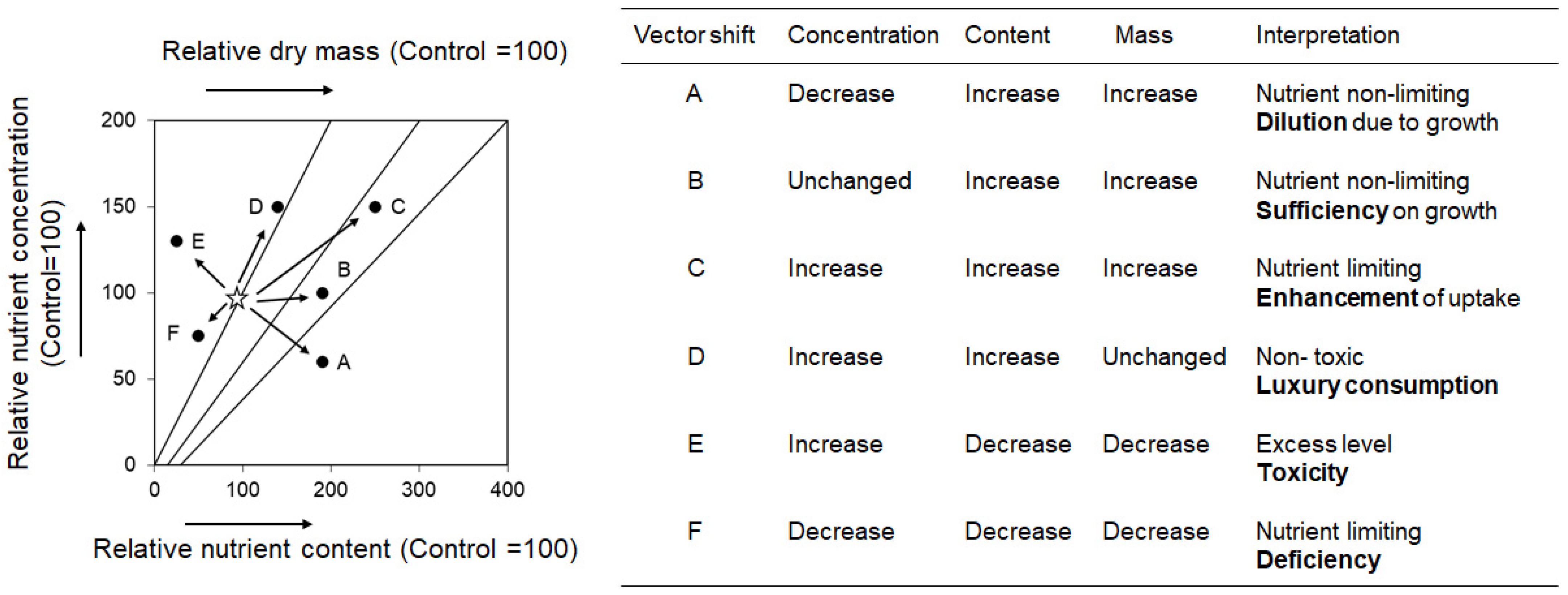
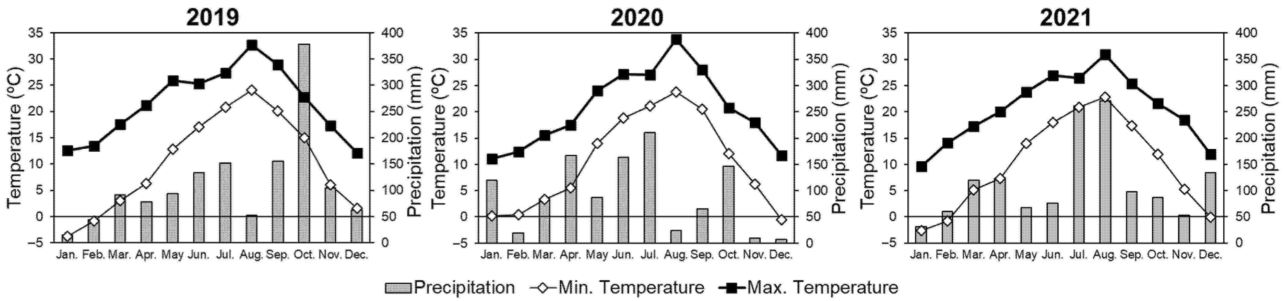
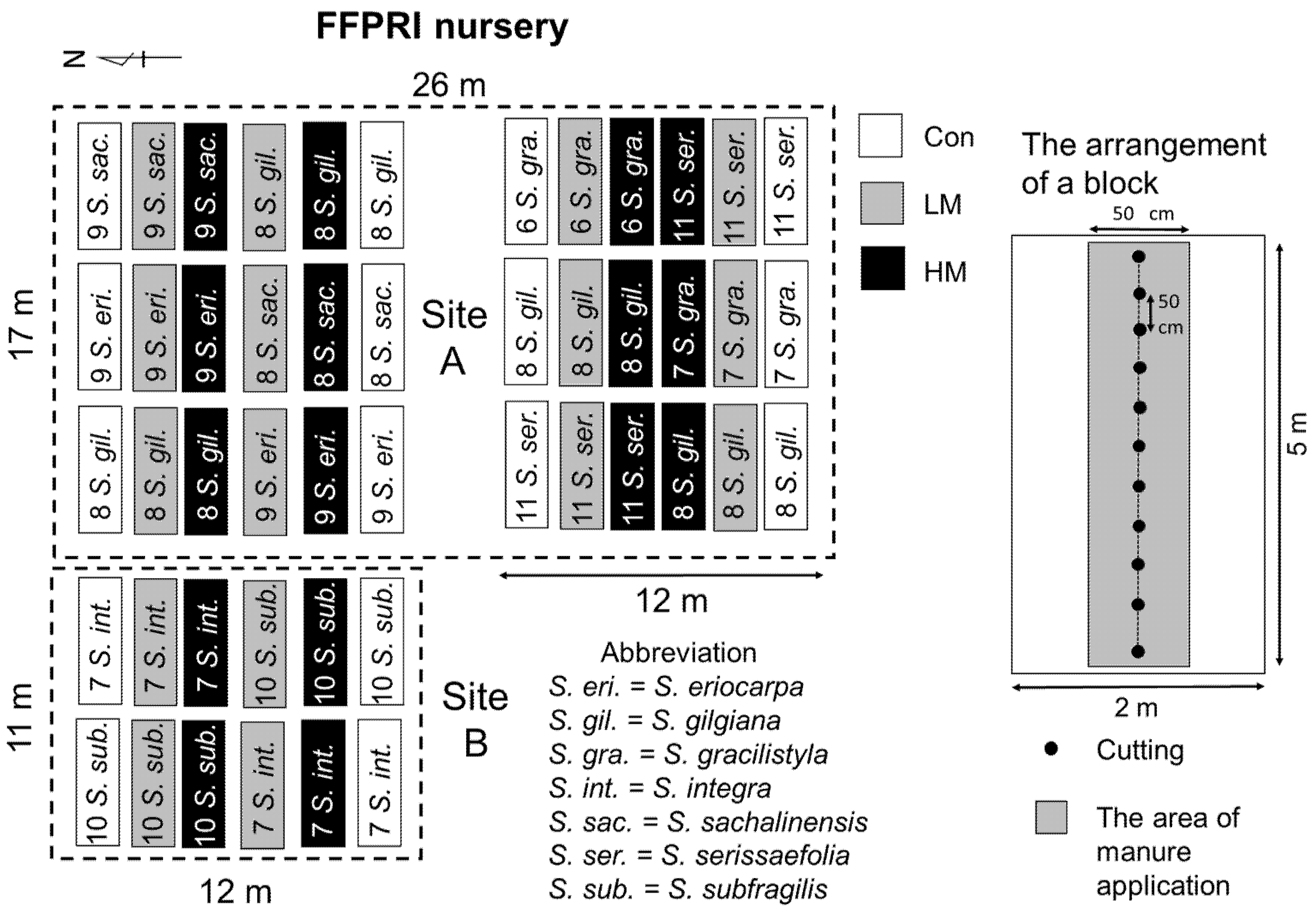
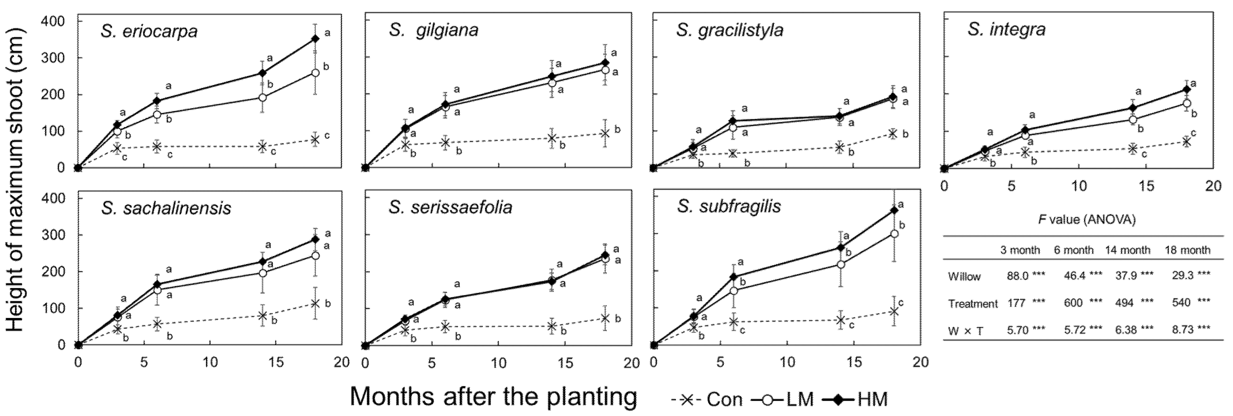
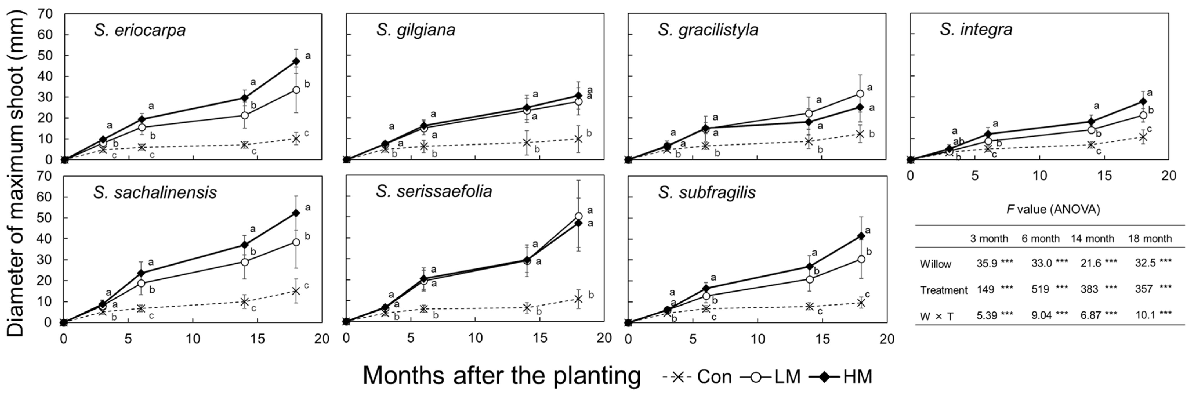
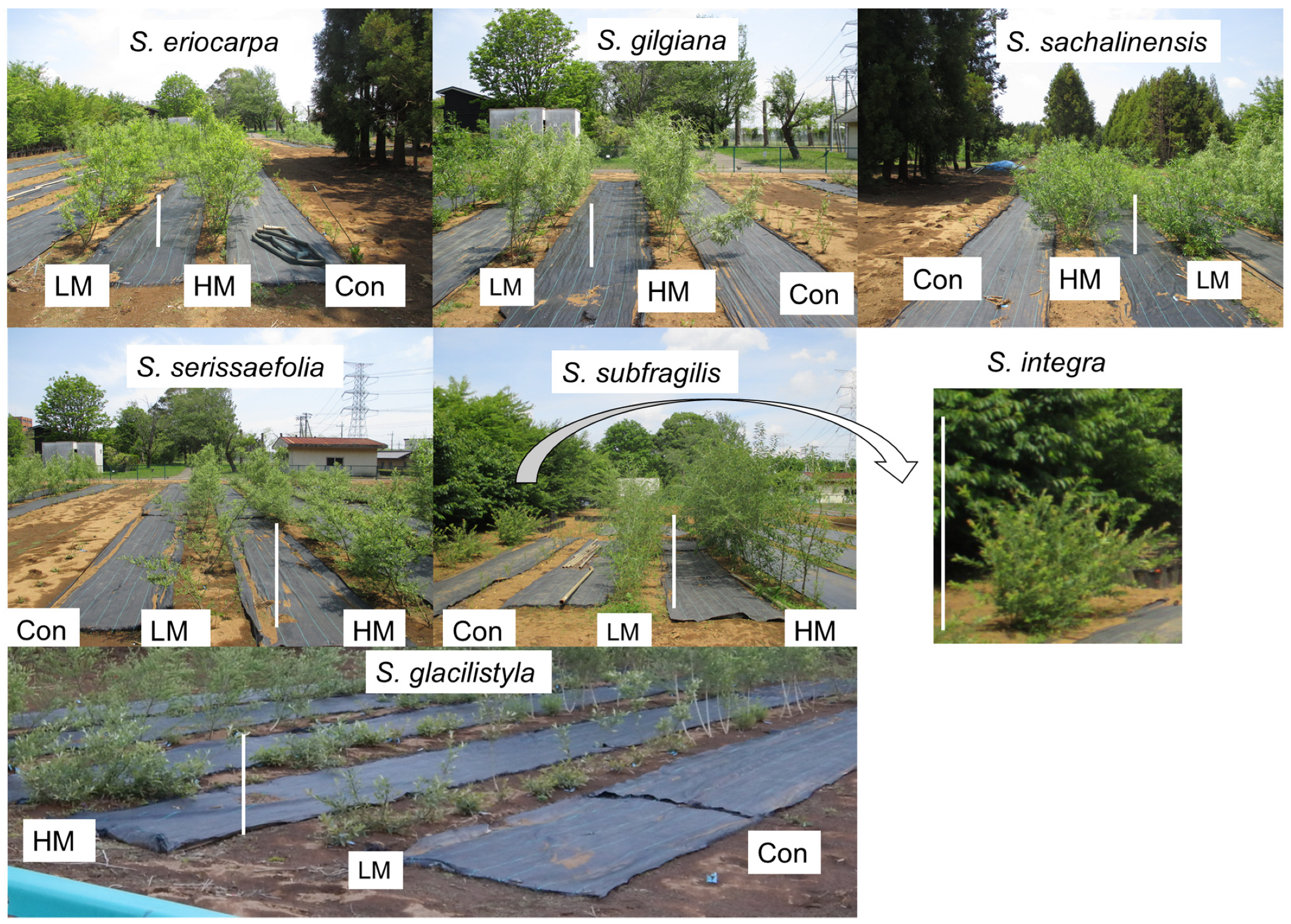
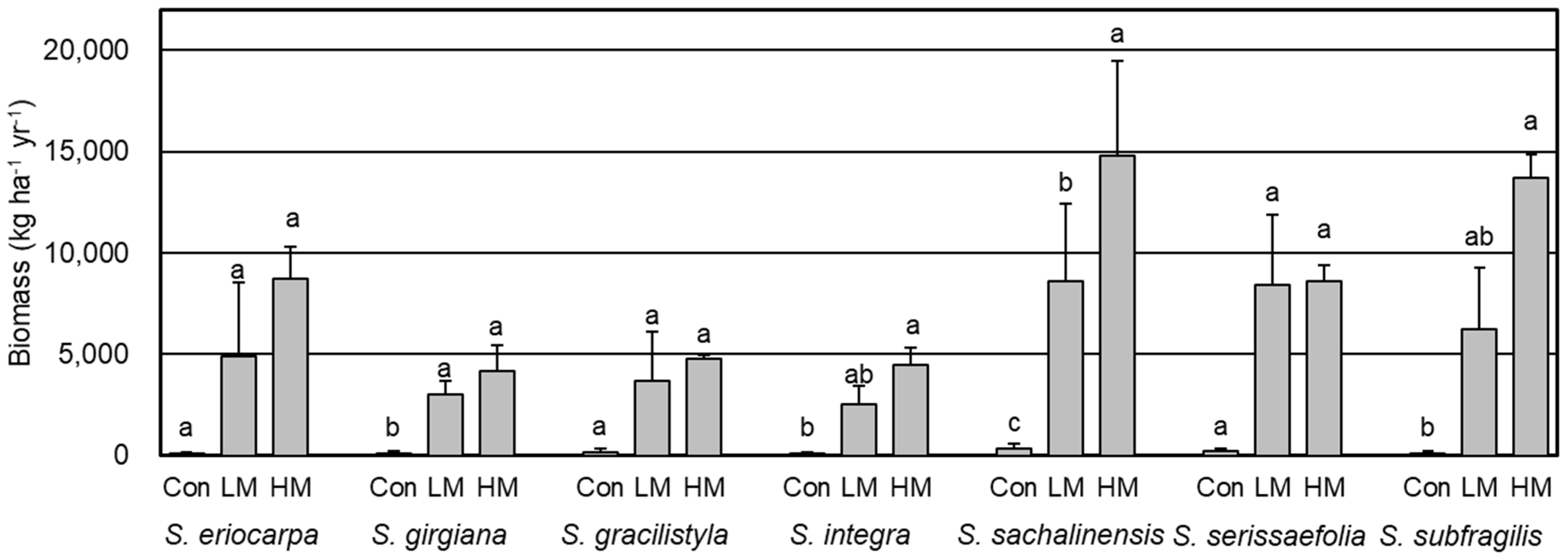
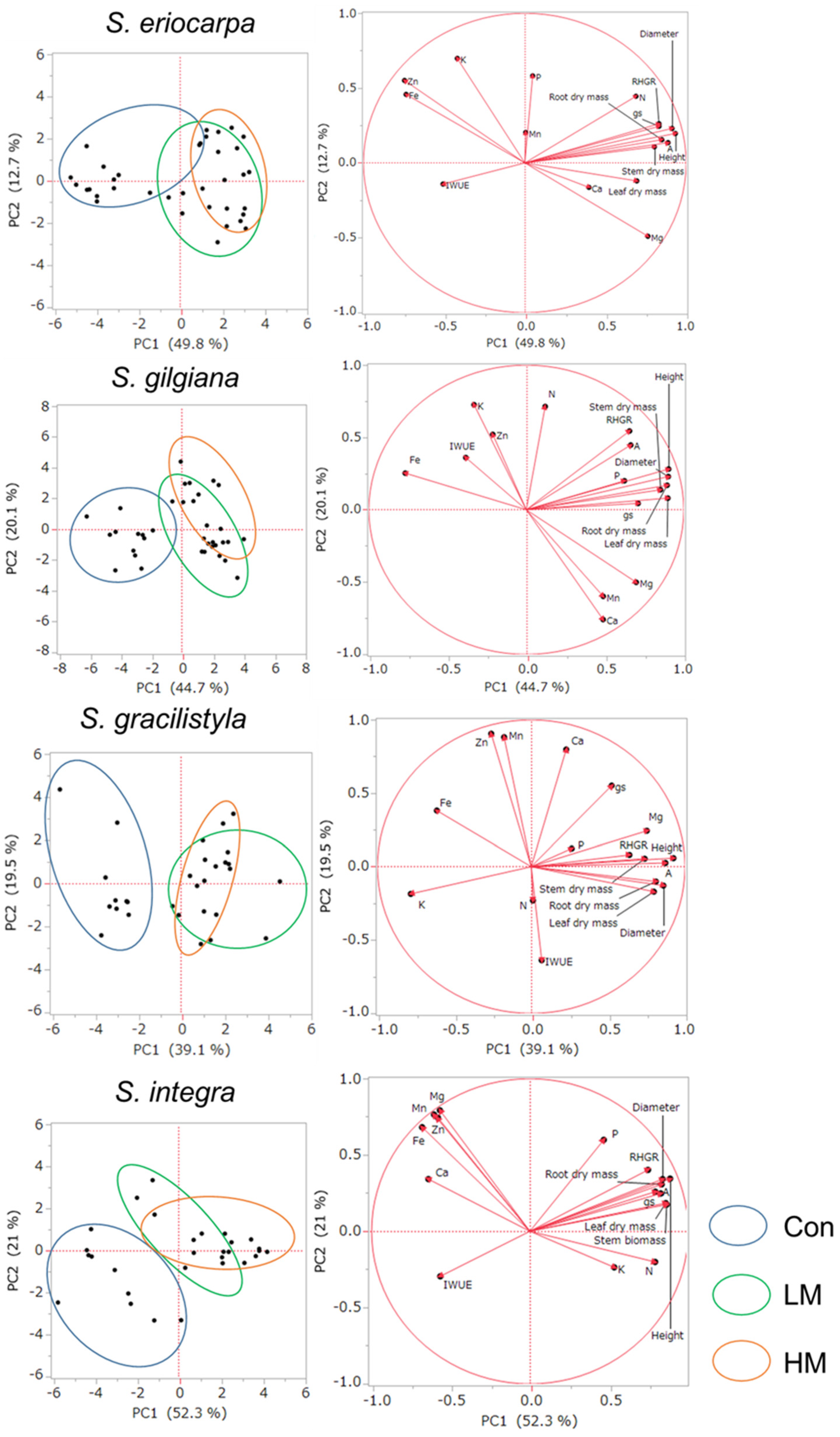
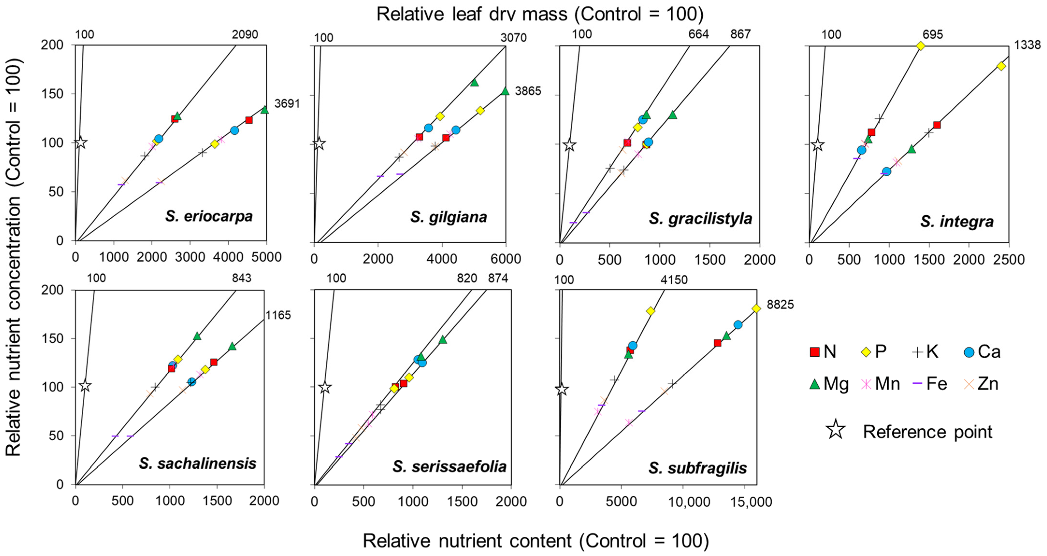
Table 1.
Habitat, range of distribution, and the geographical sources of the seven willow species used to generate cuttings for planting in the nursery.
Table 1.
Habitat, range of distribution, and the geographical sources of the seven willow species used to generate cuttings for planting in the nursery.
| Willow | Habitat | The Source Location of Cuttings (Latitude and Longitude) |
|---|---|---|
| S. eriocarpa | North-east China, far eastern Russia, Korea, and Japan (Honshu, Shikoku, and Kyushu) (1,2) | Kokai river (35°59′ N, 134°00′ E) |
| S. gilgiana | Korea and Japan (Honshu) (2,3) | Sugao marsh (36°00′ N, 139°55′ E) |
| S. gracilistyla | Far eastern Russia, northeast China, Korea, and Japan (3) | Kuji river (36°44′ N, 140°23′ E) |
| S. integra | Inner Mongolia, Korea, Japan, and far eastern Russia (3) | Naka river (36°33′ N, 140°18′ E) |
| S. sachalinensis | North-east China, Korea, Japan (Hokkaido, Honshu, Shikoku), and far eastern Russia (1,3) | Kuji river (36°47′ N, 140°22′ E) |
| S. serissaefolia | Japan (Honshu) (3) | Naka river (36°33′ N, 140°18′ E) |
| S. subfragilis | Japan, Korea, far eastern Russia, and China (3,4) | Kokai river (36°01′ N, 134°00′ E) |
Table 2.
Chemical properties of soils after treatments in Site A (n = 12), Site B (n = 4), and compost (n = 4) (mean ± SD). Asterisks indicate significant differences among three treatments, two sites, and their interaction (T × S) calculated by ANOVA. ** = p < 0.01 and *** = p < 0.001.
Table 2.
Chemical properties of soils after treatments in Site A (n = 12), Site B (n = 4), and compost (n = 4) (mean ± SD). Asterisks indicate significant differences among three treatments, two sites, and their interaction (T × S) calculated by ANOVA. ** = p < 0.01 and *** = p < 0.001.
| Parameter | Treatment | Site A | Site B | F Value (ANOVA) | ||||
|---|---|---|---|---|---|---|---|---|
| pH | Con | 5.59 ± 0.13 | c | 5.70 ± 0.06 | c | Treatment | 159 | *** |
| LM | 6.29 ± 0.07 | b | 6.31 ± 0.13 | b | Site | 2.5 | n.s. | |
| HM | 6.66 ± 0.22 | a | 6.78 ± 0.20 | a | T × S | 0.4 | n.s. | |
| Compost | 7.36 ± 0.04 | |||||||
| C (mol kg−1) | Con | 2.98 ± 0.46 | c | 2.84 ± 0.09 | c | Treatment | 20.7 | *** |
| LM | 4.35 ± 0.96 | b | 3.89 ± 0.10 | b | Site | 3.5 | n.s. | |
| HM | 6.04 ± 1.53 | a | 4.84 ± 0.44 | a | T × S | 0.9 | n.s. | |
| Compost | 28.8 ± 0.3 | (34.4%) | ||||||
| N (mmol kg−1) | Con | 193 ± 21 | c | 186 ± 5 | c | Treatment | 35.8 | *** |
| LM | 293 ± 44 | b | 276 ± 8 | b | Site | 2.3 | n.s. | |
| HM | 410 ± 93 | a | 351 ± 48 | a | T × S | 0.5 | n.s. | |
| Compost | 2344 ± 53 | (3.28%) | ||||||
| P (mmol kg−1) | Con | 1.4 ± 0.5 | c | 1.5 ± 0.2 | c | Treatment | 187 | *** |
| LM | 39.0 ± 14.6 | b | 48.3 ± 4.5 | b | Site | 4.0 | n.s. | |
| HM | 77.0 ± 12.1 | a | 88.2 ± 12.1 | a | T × S | 1.0 | n.s. | |
| Compost | 4101 ± 39 | (12.7%) | ||||||
| Ca (mmol kg−1) | Con | 10.6 ± 3.5 | c | 6.9 ± 0.8 | c | Treatment | 62.6 | *** |
| LM | 26.5 ± 9.6 | b | 30.0 ± 2.8 | b | Site | 0.4 | n.s. | |
| HM | 39.6 ± 9.2 | a | 44.4 ± 6.9 | a | T × S | 1.2 | n.s. | |
| Compost | 562 ± 44 | (2.24%) | ||||||
| Mg (mmol kg−1) | Con | 1.7 ± 0.8 | c | 1.3 ± 0.1 | c | Treatment | 204 | *** |
| LM | 19.2 ± 3.3 | b | 19.2 ± 4.9 | b | Site | 0.1 | n.s. | |
| HM | 31.1 ± 4.5 | a | 30.5 ± 6.1 | a | T × S | <0.1 | n.s. | |
| Compost | 405 ± 82 | (0.98%) | ||||||
| K (mmol kg−1) | Con | 2.7 ± 0.8 | c | 2.1 ± 0.4 | c | Treatment | 139 | *** |
| LM | 25.0 ± 2.9 | b | 25.8 ± 5.3 | b | Site | 0.8 | n.s. | |
| HM | 44.6 ± 4.4 | a | 43.4 ± 5.7 | a | T × S | 0.8 | n.s. | |
| Compost | 1368 ± 91 | (5.34%) | ||||||
| Na (mmol kg−1) | Con | 2.0 ± 0.6 | c | 1.5 ± 0.1 | c | Treatment | 88.1 | *** |
| LM | 14.5 ± 6.0 | b | 22.2 ± 3.5 | b | Site | 7.5 | ** | |
| HM | 28.2 ± 8.6 | a | 36.5 ± 5.6 | a | T × S | 2.2 | n.s. | |
| Compost | 265 ± 19 | (0.61%) | ||||||
| Mn (µmol kg−1) | Con | 118 ± 33 | b | 111 ± 3 | c | Treatment | 12.8 | *** |
| LM | 150 ± 24 | a | 141 ± 3 | b | Site | 1.1 | n.s. | |
| HM | 171 ± 26 | a | 161 ± 4 | a | T × S | <0.1 | n.s. | |
| Compost | 2389 ± 141 | (131 ppm) | ||||||
| Fe (µmol kg−1) | Con | 92.3 ± 19.7 | a | 93.4 ± 12.6 | a | Treatment | 80.8 | *** |
| LM | 41.6 ± 7.8 | b | 42.2 ± 5.7 | b | Site | <0.1 | n.s. | |
| HM | 34.9 ± 7.5 | b | 35.3 ± 4.8 | b | T × S | <0.1 | n.s. | |
| Compost | 588 ± 35 | (33 ppm) | ||||||
| Zn (µmol kg−1) | Con | 19 ± 7 | c | 15 ± 2 | c | Treatment | 50.2 | *** |
| LM | 304 ± 108 | b | 244 ± 35 | b | Site | 2.5 | n.s. | |
| HM | 453 ± 152 | a | 363 ± 52 | a | T × S | 0.6 | n.s. | |
| Compost | 2065 ± 199 | (1350 ppm) | ||||||
Note. The ratio of compost and water for the measurement of pH was 1:5. Different alphabetical letters indicate significant differences between the three treatments based on by Tukey test (p < 0.05).
Table 3.
Survival rates of individuals, number of stems per individual and RHGR for the individual of seven willows grown under three treatments (mean ± SD except for survival). Asterisks indicate significant differences among seven willows, three treatments, and their interaction (W × T) calculated by ANOVA. ** = p < 0.01 and *** = p < 0.001.
| Species | Treatment | Survival (%) | Stems | RHGR (cm cm−1yr−1) | ||
|---|---|---|---|---|---|---|
| S. eriocarpa (n = 18) | Con | 100 | 1.94 ± 0.73 | b | 0.354 ± 0.180 | b |
| LM | 100 | 3.22 ± 1.31 | a | 0.632 ± 0.178 | a | |
| HM | 100 | 3.11 ± 1.23 | a | 0.694 ± 0.064 | a | |
| S. gilgiana (n = 32) | Con | 75 | 2.18 ± 0.90 | a | 0.396 ± 0.263 | b |
| LM | 88 | 2.34 ± 0.96 | a | 0.604 ± 0.124 | a | |
| HM | 94 | 2.31 ± 0.99 | a | 0.640 ± 0.146 | a | |
| S. gracilistyla (n = 13) | Con | 69 | 4.22 ± 2.39 | a | 0.387 ± 0.282 | b |
| LM | 92 | 4.00 ± 2.00 | a | 0.686 ± 0.254 | a | |
| HM | 69 | 3.40 ± 1.90 | a | 0.767 ± 0.232 | a | |
| S. integra (n = 14) | Con | 73 | 1.72 ± 0.79 | b | 0.397 ± 0.163 | b |
| LM | 79 | 3.00 ± 1.48 | a | 0.711 ± 0.131 | a | |
| HM | 86 | 3.00 ± 0.95 | a | 0.769 ± 0.108 | a | |
| S. sachalinensis (n = 17) | Con | 82 | 2.67 ± 1.15 | a | 0.405 ± 0.143 | b |
| LM | 71 | 2.64 ± 1.43 | a | 0.791 ± 0.115 | a | |
| HM | 65 | 2.73 ± 1.56 | a | 0.750 ± 0.092 | a | |
| S. serissaefolia (n = 22) | Con | 68 | 4.64 ± 2.73 | a | 0.484 ± 0.314 | b |
| LM | 82 | 3.31 ± 1.45 | a | 0.779 ± 0.187 | a | |
| HM | 82 | 3.00 ± 2.13 | a | 0.781 ± 0.088 | a | |
| S. subfragilis (n = 20) | Con | 70 | 2.07 ± 1.16 | a | 0.302 ± 0.175 | b |
| LM | 80 | 2.53 ± 0.83 | a | 0.861 ± 0.142 | a | |
| HM | 95 | 2.78 ± 1.31 | a | 0.938 ± 0.148 | a | |
| F value (ANOVA) | Willow | 12.0 | *** | 12.0 | *** | |
| Treatment | 0.72 | n.s. | 86.3 | *** | ||
| W × T | 2.52 | ** | 6.77 | *** |
Note. Survival rates and number of stems were calculated at 18 months after planting. Different letters indicate significant differences between the three treatments based on Tukey test (p < 0.05).
Table 4.
Photosynthetic rate at light saturation (A), stomatal conductance (gs) and intrinsic water use efficiency (IWUE) of the leaves of individuals of seven willows grown under three treatments (mean ± SD). Asterisks indicate significant differences among seven willows, three treatments, and their interaction (W × T) calculated by ANOVA. * = p < 0.05 and *** = p < 0.001.
| Species | Treatment | A (µmol m−2s−1) | gs (mol m−2s−1) | IWUE (µmol mol−1) | |||
|---|---|---|---|---|---|---|---|
| S. eriocarpa (n = 12) | Con | 11.2 ± 2.6 | b | 0.502 ± 0.222 | b | 25.6 ± 11.0 | a |
| LM | 18.5 ± 1.6 | a | 1.061 ± 0.113 | a | 17.7 ± 2.7 | b | |
| HM | 19.4 ± 1.7 | a | 1.064 ± 0.237 | a | 18.9 ± 3.2 | ab | |
| S. gilgiana (n = 12) | Con | 14.4 ± 4.0 | b | 0.339 ± 0.130 | b | 45.2 ± 8.8 | a |
| LM | 18.7 ± 1.9 | a | 0.461 ± 0.087 | a | 41.8 ± 7.7 | a | |
| HM | 20.3 ± 2.5 | a | 0.494 ± 0.081 | a | 42.6 ± 11.1 | a | |
| S. gracilistyla (n = 9) | Con | 13.7 ± 2.2 | b | 0.651 ± 0.217 | b | 22.2 ± 4.8 | a |
| LM | 21.1 ± 2.0 | a | 0.977 ± 0.338 | a | 24.0 ± 8.1 | a | |
| HM | 20.5 ± 1.0 | a | 0.971 ± 0.359 | a | 24.4 ± 10.4 | a | |
| S. integra (n = 10) | Con | 6.9 ± 3.1 | b | 0.274 ± 0.168 | b | 28.6 ± 11.6 | a |
| LM | 15.1 ± 2.3 | a | 0.833 ± 0.222 | a | 18.8 ± 3.7 | b | |
| HM | 16.2 ± 3.6 | a | 0.834 ± 0.275 | a | 20.7 ± 5.5 | ab | |
| S. sachalinensis (n = 11) | Con | 13.5 ± 1.8 | b | 0.336 ± 0.208 | a | 45.3 ± 3.5 | a |
| LM | 19.8 ± 2.8 | a | 0.511 ± 0.201 | a | 52.2 ± 4.6 | a | |
| HM | 20.8 ± 1.9 | a | 0.537 ± 0.272 | a | 53.4 ± 3.2 | a | |
| S. serissaefolia (n = 12) | Con | 14.4 ± 3.6 | b | 0.467 ± 0.133 | a | 33.1 ± 12.6 | a |
| LM | 22.4 ± 3.3 | a | 0.567 ± 0.172 | a | 39.3 ± 7.6 | a | |
| HM | 20.8 ± 1.9 | a | 0.621 ± 0.160 | a | 41.4 ± 9.7 | a | |
| S. subfragilis (n = 12) | Con | 11.3 ± 1.4 | b | 0.429 ± 0.163 | b | 29.0 ± 10.8 | a |
| LM | 24.2 ± 2.4 | a | 1.291 ± 0.565 | a | 21.1 ± 6.3 | b | |
| HM | 24.3 ± 2.3 | a | 1.009 ± 0.351 | a | 25.7 ± 5.4 | ab | |
| F value (ANOVA) | Willow | 31.4 | *** | 23.7 | *** | 45.1 | *** |
| Treatment | 284 | *** | 59.2 | *** | 3.80 | * | |
| W × T | 3.89 | *** | 4.14 | *** | 1.73 | n.s. | |
Note. Different alphabetical letters indicate significant differences between the three treatments based on Tukey test (p < 0.05).
Table 5.
Dry mass in different tissues of individuals of the seven willows grown under three treatments (mean ± SD). Asterisks indicate significant differences among seven willows, three treatments, and their interaction (W × T) calculated by ANOVA (*** = p < 0.001).
Table 5.
Dry mass in different tissues of individuals of the seven willows grown under three treatments (mean ± SD). Asterisks indicate significant differences among seven willows, three treatments, and their interaction (W × T) calculated by ANOVA (*** = p < 0.001).
| Species | Treatment | Leaf (g) | Stem & Branch (g) | Root (g) | |||
|---|---|---|---|---|---|---|---|
| S. eriocarpa (n = 12) | Con | 10 ± 5 | c | 15 ± 6 | c | 25 ± 15 | b |
| LM | 214 ± 97 | b | 1255 ± 3911 | b | 586 ± 383 | a | |
| HM | 378 ± 215 | a | 2052 ± 550 | a | 802 ± 183 | a | |
| S. gilgiana (n = 12) | Con | 10 ± 5 | b | 20 ± 11 | c | 21 ± 6 | b |
| LM | 316 ± 103 | a | 1090 ± 331 | b | 380 ± 107 | a | |
| HM | 413 ± 138 | a | 1452 ± 415 | a | 482 ± 147 | a | |
| S. gracilistyla (n = 9) | Con | 43 ± 13 | b | 58 ± 22 | b | 48 ± 15 | b |
| LM | 372 ± 220 | a | 1124 ± 892 | a | 426 ± 299 | a | |
| HM | 285 ± 140 | a | 885 ± 393 | a | 396 ± 112 | a | |
| S. integra (n = 10) | Con | 11 ± 5 | c | 27 ± 15 | c | 53 ± 18 | c |
| LM | 71 ± 40 | b | 536 ± 315 | b | 383 ± 167 | b | |
| HM | 137 ± 44 | a | 989 ± 358 | a | 635 ± 191 | a | |
| S. sachalinensis (n = 11) | Con | 53 ± 41 | c | 81 ± 62 | c | 69 ± 46 | c |
| LM | 447 ± 243 | b | 1538 ± 862 | b | 684 ± 447 | b | |
| HM | 617 ± 206 | a | 3086 ± 1417 | a | 1195 ± 504 | a | |
| S. serissaefolia (n = 12) | Con | 25 ± 23 | b | 46 ± 46 | b | 34 ± 28 | b |
| LM | 202 ± 123 | a | 2081 ± 1416 | a | 733 ± 435 | a | |
| HM | 215 ± 128 | a | 2111 ± 1100 | a | 708 ± 363 | a | |
| S. subfragilis (n = 12) | Con | 6 ± 2 | c | 26 ± 16 | c | 37 ± 14 | c |
| LM | 234 ± 125 | b | 1205 ± 857 | b | 451 ± 288 | b | |
| HM | 497 ± 228 | a | 3317 ± 1375 | a | 1030 ± 337 | a | |
| F value (ANOVA) | Willow | 16.3 | *** | 10.1 | *** | 8.45 | *** |
| Treatment | 139 | *** | 133 | *** | 154 | *** | |
| W × T | 5.35 | *** | 5.93 | *** | 4.38 | *** | |
Note. Different alphabetical letters indicate significant differences between the three treatments based on Tukey test (p < 0.05).
Table 6.
Concentrations of chemical elements N, P, K and Ca (dry mass) in the leaves of individuals of seven willows grown under three treatments (mean ± SD). Asterisks indicate significant differences among seven willows, three treatments, and their interaction (W × T) calculated by ANOVA. * = p < 0.05, ** = 0.01 and *** = p < 0.001.
| Species | Treatment | N (µmol g−1) | P (µmol g−1) | K (µmol g−1) | Ca (µmol g−1) | ||||
|---|---|---|---|---|---|---|---|---|---|
| S. eriocarpa (n = 12) | Con | 1160 ± 171 | b | 177 ± 33 | a | 251 ± 27 | a | 242 ± 59 | a |
| LM | 1445 ± 129 | a | 184 ± 29 | a | 218 ± 32 | a | 252 ± 26 | a | |
| HM | 1427 ± 170 | a | 175 ± 32 | a | 226 ± 44 | a | 273 ± 28 | a | |
| S. gilgiana (n = 12) | Con | 1460 ± 189 | a | 150 ± 32 | b | 140 ± 42 | a | 390 ± 86 | a |
| LM | 1568 ± 163 | a | 192 ± 39 | a | 121 ± 30 | a | 455 ± 141 | a | |
| HM | 1555 ± 127 | a | 201 ± 26 | a | 137 ± 38 | a | 448 ± 142 | a | |
| S. gracilistyla (n = 9) | Con | 1450 ± 93 | a | 143 ± 14 | b | 304 ± 32 | a | 271 ± 57 | b |
| LM | 1450 ± 78 | a | 144 ± 16 | b | 225 ± 45 | b | 277 ± 54 | ab | |
| HM | 1472 ± 87 | a | 168 ± 18 | a | 229 ± 46 | b | 339 ± 60 | a | |
| S. integra (n = 10) | Con | 1215 ± 206 | a | 128 ± 26 | b | 280 ± 70 | b | 286 ± 113 | a |
| LM | 1365 ± 198 | a | 258 ± 75 | a | 354 ± 70 | a | 269 ± 57 | a | |
| HM | 1455 ± 254 | a | 230 ± 45 | a | 313 ± 44 | ab | 207 ± 40 | a | |
| S. sachalinensis (n = 11) | Con | 1131 ± 129 | b | 190 ± 70 | a | 186 ± 28 | a | 158 ± 51 | a |
| LM | 1369 ± 198 | a | 244 ± 65 | a | 186 ± 52 | a | 194 ± 48 | a | |
| HM | 1420 ± 170 | a | 224 ± 53 | a | 194 ± 26 | a | 167 ± 42 | a | |
| S. serissaefolia (n = 12) | Con | 1423 ± 170 | a | 135 ± 56 | a | 182 ± 33 | a | 246 ± 35 | b |
| LM | 1424 ± 138 | a | 134 ± 17 | a | 149 ± 22 | b | 315 ± 50 | a | |
| HM | 1473 ± 82 | a | 149 ± 32 | a | 140 ± 23 | b | 308 ± 43 | a | |
| S. subfragilis (n = 12) | Con | 1250 ± 348 | b | 113 ± 15 | b | 514 ± 148 | a | 132 ± 51 | b |
| LM | 1723 ± 173 | a | 201 ± 49 | a | 551 ± 53 | a | 188 ± 42 | a | |
| HM | 1814 ± 118 | a | 204 ± 30 | a | 532 ± 52 | a | 217 ± 63 | a | |
| F value (ANOVA) | Willow | 13.8 | *** | 15.9 | *** | 236 | *** | 56.6 | *** |
| Treatment | 37.5 | *** | 32.4 | *** | 1.07 | n.s. | 6.00 | ** | |
| W × T | 4.41 | *** | 4.68 | *** | 2.73 | ** | 2.13 | * | |
Note. Different alphabetical letters indicate significant differences between the three treatments based on Tukey test (p < 0.05).
Table 7.
Concentrations of chemical elements Mg, Mn, Fe and Zn (dry mass) in the leaves of individuals of seven willows grown under three treatments (mean ± SD). Asterisks indicate significant differences among seven willows, three treatments, and their interaction (W × T) calculated by ANOVA. * = p < 0.05, ** = 0.01 and *** = p < 0.001.
| Species | Treatment | Mg (µmol g−1) | Mn (µmol g−1) | Fe (µmol g−1) | Zn (µmol g−1) | ||||
|---|---|---|---|---|---|---|---|---|---|
| S. eriocarpa (n = 12) | Con | 92 ± 10 | b | 2.44 ± 0.89 | a | 1.96 ± 0.42 | a | 1.57 ± 0.31 | a |
| LM | 118 ± 18 | a | 2.35 ± 0.21 | a | 1.12 ± 0.41 | b | 0.97 ± 0.32 | b | |
| HM | 124 ± 15 | a | 2.53 ± 0.42 | a | 1.16 ± 0.35 | b | 0.96 ± 0.29 | b | |
| S. gilgiana (n = 12) | Con | 112 ± 22 | b | 1.42 ± 0.11 | a | 1.62 ± 0.30 | a | 1.17 ± 0.22 | a |
| LM | 183 ± 63 | a | 1.50 ± 0.19 | a | 1.09 ± 0.32 | b | 1.08 ± 0.26 | a | |
| HM | 173 ± 41 | a | 1.56 ± 0.31 | a | 1.12 ± 0.21 | b | 1.15 ± 0.39 | a | |
| S. gracilistyla (n = 9) | Con | 101 ± 11 | a | 2.17 ± 0.68 | a | 11.4 ± 12.6 | a | 1.42 ± 0.80 | a |
| LM | 95 ± 12 | b | 1.96 ± 0.35 | a | 3.5 ± 1.6 | ab | 1.00 ± 0.39 | a | |
| HM | 124 ± 17 | a | 2.23 ± 0.35 | a | 2.3 ± 1.1 | b | 1.34 ± 0.43 | a | |
| S. integra (n = 10) | Con | 108 ± 33 | a | 3.81 ± 2.31 | a | 3.28 ± 2.12 | a | 2.53 ± 1.28 | a |
| LM | 114 ± 47 | a | 3.84 ± 2.56 | a | 2.79 ± 2.74 | a | 2.54 ± 1.17 | a | |
| HM | 104 ± 41 | a | 3.11 ± 2.23 | a | 2.29 ± 2.29 | a | 2.11 ± 1.09 | a | |
| S. sachalinensis (n = 11) | Con | 63 ± 15 | b | 2.58 ± 0.74 | a | 3.32 ± 1.65 | a | 0.85 ± 0.07 | a |
| LM | 97 ± 23 | a | 3.17 ± 0.62 | a | 1.65 ± 0.76 | b | 0.79 ± 0.10 | a | |
| HM | 90 ± 23 | a | 2.92 ± 0.50 | a | 1.65 ± 0.57 | b | 0.83 ± 0.67 | a | |
| S. serissaefolia (n = 12) | Con | 92 ± 14 | b | 3.94 ± 0.96 | a | 15.7 ± 7.9 | a | 1.33 ± 0.53 | a |
| LM | 121 ± 19 | a | 2.83 ± 0.69 | b | 6.6 ± 5.1 | b | 0.78 ± 0.29 | b | |
| HM | 137 ± 22 | a | 2.46 ± 0.66 | b | 4.4 ± 4.3 | b | 0.64 ± 0.32 | b | |
| S. subfragilis (n = 12) | Con | 66 ± 34 | b | 4.64 ± 1.60 | a | 1.66 ± 0.42 | a | 1.48 ± 0.58 | a |
| LM | 89 ± 18 | ab | 3.48 ± 0.67 | b | 1.35 ± 0.21 | b | 1.28 ± 0.23 | a | |
| HM | 101 ± 11 | a | 2.96 ± 0.42 | b | 1.25 ± 0.14 | b | 1.42 ± 0.20 | a | |
| F value (ANOVA) | Willow | 27.8 | *** | 19.7 | *** | 22.6 | *** | 29.6 | *** |
| Treatment | 36.6 | *** | 3.90 | * | 22.2 | *** | 6.84 | ** | |
| W × T | 2.27 | * | 2.24 | * | 5.34 | *** | 1.35 | n.s. | |
Note. Different alphabetical letters indicate significant differences between the three treatments based on Tukey test (p < 0.05).
Table 8.
Regression correlation coefficients between RHGR (dependent variable) and concentrations of elements in the leaves (independent variable) of willow individuals.
Table 8.
Regression correlation coefficients between RHGR (dependent variable) and concentrations of elements in the leaves (independent variable) of willow individuals.
| Species | Element | r | F | Element | r | F |
|---|---|---|---|---|---|---|
| S. eriocarpa (n = 36) | N | 0.611 | 20.2 *** | Mg | 0.484 | 10.4 ** |
| P | 0.068 | 0.16 | Mn | −0.052 | 0.09 | |
| K | −0.040 | 0.05 | Fe | −0.536 | 13.7 *** | |
| Ca | 0.130 | 0.58 | Zn | −0.548 | 14.6 *** | |
| S. gilgiana (n = 36) | N | 0.415 | 7.07 * | Mg | 0.209 | 1.55 |
| P | 0.592 | 18.3 *** | Mn | −0.028 | 0.03 | |
| K | 0.199 | 1.41 | Fe | −0.406 | 6.52 * | |
| Ca | −0.054 | 0.10 | Zn | 0.006 | <0.01 | |
| S. gracilistyla (n = 27) | N | −0.012 | <0.01 | Mg | 0.572 | 13.6 *** |
| P | 0.463 | 7.62 * | Mn | −0.121 | 0.40 *** | |
| K | −0.434 | 6.51 * | Fe | −0.480 | 8.10 ** | |
| Ca | 0.186 | 1.01 | Zn | −0.183 | 0.93 | |
| S. integra (n = 30) | N | 0.469 | 7.91 ** | Mg | −0.068 | 0.13 |
| P | 0.540 | 11.6 ** | Mn | −0.157 | 0.68 | |
| K | 0.286 | 2.50 | Fe | −0.254 | 1.86 | |
| Ca | −0.331 | 3.45 | Zn | −0.168 | 0.79 | |
| S. sachalinensis (n = 33) | N | 0.470 | 8.77 ** | Mg | 0.613 | 18.7 *** |
| P | 0.541 | 12.8 ** | Mn | 0.274 | 2.52 | |
| K | 0.141 | 0.63 | Fe | −0.575 | 15.3 *** | |
| Ca | 0.403 | 6.03 * | Zn | −0.042 | 0.05 | |
| S. serissaefolia (n = 36) | N | 0.167 | 0.98 | Mg | 0.372 | 5.47 * |
| P | 0.375 | 5.57 * | Mn | −0.261 | 2.42 | |
| K | −0.198 | 1.40 | Fe | −0.369 | 5.19 * | |
| Ca | 0.392 | 6.19 * | Zn | −0.313 | 3.59 | |
| S. subfragilis (n = 36) | N | 0.638 | 23.4 *** | Mg | 0.466 | 9.42 ** |
| P | 0.720 | 36.6 *** | Mn | −0.471 | 9.70 ** | |
| K | 0.024 | 0.02 | Fe | −0.431 | 7.75 ** | |
| Ca | 0.583 | 17.5 *** | Zn | 0.013 | <0.01 |
Note. * p < 0.05, ** p < 0.01, and *** p < 0.001.
Disclaimer/Publisher’s Note: The statements, opinions and data contained in all publications are solely those of the individual author(s) and contributor(s) and not of MDPI and/or the editor(s). MDPI and/or the editor(s) disclaim responsibility for any injury to people or property resulting from any ideas, methods, instructions or products referred to in the content. |
© 2023 by the authors. Licensee MDPI, Basel, Switzerland. This article is an open access article distributed under the terms and conditions of the Creative Commons Attribution (CC BY) license (https://creativecommons.org/licenses/by/4.0/).
Share and Cite
MDPI and ACS Style
Kayama, M.; Kikuchi, S.; Uemura, A.; Takahashi, M. Growth Characteristics of Seven Willow Species Distributed in Eastern Japan in Response to Compost Application. Forests 2023, 14, 606. https://doi.org/10.3390/f14030606
AMA Style
Kayama M, Kikuchi S, Uemura A, Takahashi M. Growth Characteristics of Seven Willow Species Distributed in Eastern Japan in Response to Compost Application. Forests. 2023; 14(3):606. https://doi.org/10.3390/f14030606
Chicago/Turabian StyleKayama, Masazumi, Satoshi Kikuchi, Akira Uemura, and Masayoshi Takahashi. 2023. "Growth Characteristics of Seven Willow Species Distributed in Eastern Japan in Response to Compost Application" Forests 14, no. 3: 606. https://doi.org/10.3390/f14030606
Note that from the first issue of 2016, this journal uses article numbers instead of page numbers. See further details here.