Article

Identification of Pine Wilt Disease Infected Wood Using UAV RGB Imagery and Improved YOLOv5 Models Integrated with Attention Mechanisms

1
College of Science, Anhui Agricultural University, Hefei 230036, China
2
Laboratory of Sensors, Ministry of Agriculture and Rural Affairs, Hefei 230036, China
3
Precision Forestry Key Laboratory of Beijing, School of Forestry, Beijing Forestry University, Beijing 100083, China
4
Chinese Academy of Surveying & Mapping, Beijing 100091, China
5
Institute of Agricultural Information, Chinese Academy of Agricultural Sciences, Beijing 100091, China
6
Anhui Vocational and Technical College of Industrial Economy, Hefei 230051, China
*
Authors to whom correspondence should be addressed.
These authors contributed equally to this work.
Forests 2023, 14(3), 588; https://doi.org/10.3390/f14030588
Submission received: 17 January 2023 / Revised: 6 March 2023 / Accepted: 14 March 2023 / Published: 16 March 2023

Abstract

:
Pine wilt disease (PWD) is a great danger, due to two aspects: no effective cure and fast dissemination. One key to the prevention and treatment of pine wilt disease is the early detection of infected wood. Subsequently, appropriate treatment can be applied to limit the further spread of pine wilt disease. In this work, a UAV (Unmanned Aerial Vehicle) with a RGB (Red, Green, Blue) camera was employed as it provided high-quality images of pine trees in a timely manner. Seven flights were performed above seven sample plots in northwestern Beijing, China. Then, raw images captured by the UAV were further pre-processed, classified, annotated, and formed the research datasets. In the formal analysis, improved YOLOv5 frameworks that integrated four attention mechanism modules, i.e., SE (Squeeze-and-Excitation), CA (Coordinate Attention), ECA (Efficient Channel Attention), and CBAM (Convolutional Block Attention Module), were developed. Each of them had been shown to improve the overall identification rate of infected trees at different ranges. The CA module was found to have the best performance, with an accuracy of 92.6%, a 3.3% improvement over the original YOLOv5s model. Meanwhile, the recognition speed was improved by 20 frames/second compared to the original YOLOv5s model. The comprehensive performance could well support the need for rapid detection of pine wilt disease. The overall framework proposed by this work shows a fast response to the spread of PWD. In addition, it requires a small amount of financial resources, which determines the duplication of this method for forestry operators.

1. Introduction

Pine wilt disease (PWD) is a forest disease caused by the pine wood nematode. PWD was first discovered in China in 1982. Currently, PWD is spreading rapidly in China. Therefore, PWD is listed as a significant invasive alien species in China [1]. Meanwhile, PWD is also included in the phytosanitary list [2,3]. Technically, when a pine tree is infected by PWD, it is defined as infected wood. An infected wood will have a distinct look in four phases and different biological properties when compared to healthy trees [4]. In the first stage of being infected with PWD, there will be fewer noticeable changes. Simultaneously, the resin secretion inside pines will start to decrease. In the second stage, the needles in the crown will lose their luster, and the crown part of the tree will turn yellow or red. At the same time, the resin secretion will cease. In the third stage, the infected wood will start to die off. In the fourth and last stage, the needles of the entire canopy will turn from yellow to brown until the end of physical activities [5].
PWD is highly contagious. The early detection of PWD is the key to the prevention and control of this disease [6]. There are many methods to identify PWD nowadays. A major approach is manual visual interpretation in field surveys, which has a lower financial and technical requirement [7]. Generally speaking, the infected wood is determined by observing changes in the appearance of pine trees using the eyes of crew members [8,9]. One problem is that manual interpretation is inefficient and highly subjective. Meanwhile, it is hard to be applied if we have to monitor large areas of forests [10]. Therefore, it is necessary to develop an objective and efficient method for the early detection of PWD.
Instead of manual interpretation, ground experiments and remote sensing methods were employed to monitor PWD [7]. Beyond the visual appearance, ground experiments can accurately measure the spectral information of plants and can be used to provide precise references to remote sensing approaches. For example, Kim et al. collected leaf reflection spectra of the infected wood. The best indicator for the detection of spectral reflectance characteristics of black pine forests was determined [11]. Lee et al. used a ground-based hyperspectral sensor to analyze the band changes of the infected wood at different stages [12]. The results showed that the greatest magnitude of vegetation index change was observed at 688 nm wavelength. Xue et al. analyzed the spectral bands to determine the light conditions and growth environment of different trees in the woodland [13].
After gaining experience provided by ground experiments, people can use remote sensing methods for large-area monitoring [6]. From the perspective of data sources, we divide remote sensing methods into two categories. The first category is the satellite/manned aircraft remote sensing methods using public data sources. These data sources are usually used to monitor large areas of forests, being multi-band and multi-temporal [14]. For example, Zhang et al. integrated high-resolution satellite image data, spectral data, and temporal and spatial feature information. This study constructed criteria for the infected wood that could improve the detection accuracy [15]. A method based on the simulation of an extended stochastic radiative transfer model for forest pests and diseases was proposed by Li et al. This method allowed the extraction of infected wood in two phases of medium-resolution satellite images [16]. Wang et al. used Gaofen-2 remote sensing images to construct a dataset of discolored standing tree samples of PWD. The recall rate of PWD discolored standing tree monitoring in the study area was 80.09% [17]. Li et al. proposed an approach to retrieve PWD-infected areas from medium-resolution satellite images of two phases based on the simulations of an extended stochastic radiative transfer model for forests infected by pests [16].
As mentioned, one characteristic of PWD is its rapid spread speed [18]. Owing to this fact, a major drawback of public data sources is the lack of real-time availability. For this problem, a UAV (Unmanned Aerial Vehicle) can acquire images of the target area in a short period of time. Therefore, we can take advantage of this to conduct forest surveys quickly [19]. Compared to multispectral and radar sensors, data images acquired by optical RGB (red, green, blue) cameras are easier to process and analyze. Meanwhile, optical RGB (Red, Green, Blue) cameras are mounted on the UAV with a great numbers. The data structure of RGB images is different from multispectral and SAR data. Therefore, novel tools, such as machine learning techniques, are widely employed [13,20]. For example, Yu et al. used YOLOv4 (You Only Look Once v4) and a Faster-R-CNN (Regions with Convolutional Neural Network features) algorithm for data processing. The detection rate was improved by taking into account the influence of broadleaf trees on the recognition of infected wood [21]. A PWD identification network SCANet (spatial-context-attention network) was proposed by Qin et al. In this study, the overall accuracy was 79% [22]. An end-to-end automatic pest detection framework was designed based on a multi-scale attention-UNet (MA-UNet) model. It achieved a recall rate of 57.38% [23]. Hu et al. used Mask R-CNN with multitasking capability as a backbone network to build a monitoring model. An improved multiscale receptive field block module was added to Mask R-CNN to extract detailed features of PWD and reduce the missed detection of PWD [24].
It is well known that the machine learning method is often used nowadays. Recent popular algorithms, such as YOLOv5, have fewer reports in the detection of PWD. Meanwhile, we noticed that the attention mechanism shows its power to enhance the original YOLOv5 frameworks in other fields of study [25]. Therefore, the attention mechanism tired of being employed in our study. Furthermore, our previous work found that the infected wood would become smaller in the images when we intended to cover a larger area with a relatively higher flight altitude. The side effects of the high cruising attitude of the UAV also had the following problems. For example, image quality is easily influenced by shading from the environment and surrounding trees; the changes of light are much more obvious; the model does not easily extract features and the recognition accuracy of the image model uses previously mentioned methods. Therefore, to overcome these problems, four YOLOv5 models with attention mechanisms were developed and tested in order to discover the current optimal solution for detecting PWD on UAV RGB images in our study. Meanwhile, the RGB camera has a low demand for financing, which facilitates its implementation in forest farms and developing regions.

2. Materials and Methods
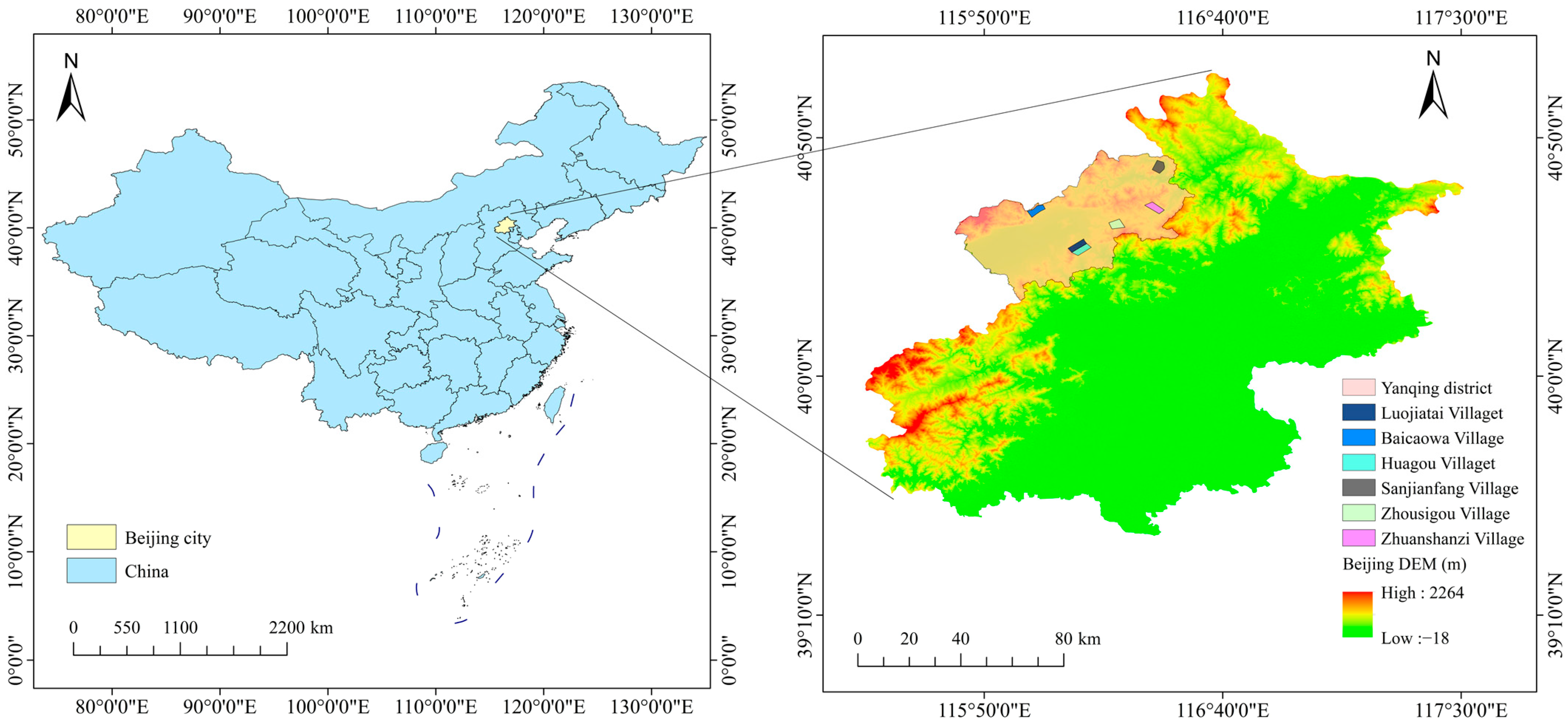
2.1. Study Area

The study area was located in Yanqing District, Beijing, China. Yanqing District is in the northwest of Beijing, with a range of 115°44′–116°34′ E and 40°16′–40°47′ N. As shown in Figure 1, the area of the study area is 1993.75 km2. Yanqing District has a large area of pine forest resources [26]. Currently, PWD is found sporadically in the study area. Before this work, the primary investigation method was manual reporting. Figure 1 shows the seven sampling locations in gray. These locations were selected by comprehensive consideration of stratified sampling and the experience of the local forest management department.

2.2. UAV Flights and Field Survey

Seven UAV flights were performed between 30 April and 30 June 2022, when the weather conditions were mild. The UAV we used was the DF-100 fixed-wing UAV [27]. The full-length is 1450 mm. The wingspan is 2430 mm. The maximum take-off weight is 18 kg. The maximum rate of climb is 6 m/s. The maximum operating altitude is 4000 m above sea level. The maximum wind resistance is class 5. The cruising speed is 70–100 km/h. Each raw image captured by the RGB camera contains four bands in the visible range.

2.2.1. Take off Check

We checked the equipment and materials used in the sortie. We checked the weather conditions to ensure the quality of aerial photography and images. We checked the air-craft, cameras and other major equipment and power systems to ensure safety.

2.2.2. Layout of Image Control Points

The control points are placed evenly in the study area as far as possible, and the control of the corners of the study area is strengthened. This can not only reduce the number of control points meeting the accuracy requirements, but also can effectively improve the accuracy all around.

2.2.3. Quality Inspection

The flight quality mainly includes image overlap, image inclination and rotation angle, route curvature and altitude, map profile coverage and zonal coverage, etc.
The specification in this paper requires that the general overlap of the heading should not be less than 53%; the general requirement of the side overlap is not less than 15%. The image film inclination angle generally cannot be greater than 5°. The maximum cannot exceed 12°. Image film rotation angle should be less than 15°. The aerial photography requires that the curvature of the route is not greater than 3%. The difference in height between adjacent images of the same route should not be greater than 30 m, and the maximum height and minimum height should not exceed 50 m. The actual height in the photography zone should not exceed 5% of the designed height. This aerial photography requires the side coverage beyond the boundary line of the area should be higher than 50% of the image width.

2.3. Data Set Preparation

2.3.1. Identification of Infected Wood

The total area of the UAV mission was 842.05 km2. Through visual interpretation, it was found that 463 woods were infected. The brief statistic of infected wood is shown in Table 1. After the pre-processing of the UAV data was completed, we found some images that were not able to be identified by visual recognition. Therefore, we conducted a field survey in order to precisely determine the tree status on those images to improve the overall confidence level of the ground truth data set.

2.3.2. Preprocessing for Imagery Consistency

The quality of images taken by the UAV is subject to many mechanical and environmental factors [28]. For example, a flight can be affected by various natural factors, such as light and wind, during data collection. These factors may cause image flaws. Therefore, it is necessary to apply a preprocessing step to those images [29]. After our flights, it was found that raw images were with different light conditions and sharpness. Therefore, it was necessary to perform corrections for light and sharpness consistency [30]. In the last step, Inpho (Trimble, Stuttgart, Germany) was used to produce the DOM (Digital Orthophoto Map) images. The overlap rate was to set to 100% and the cut rate was to set to 0–5%. After that, orthophotos of the desired size were cut out and the raw dataset was well prepared.

2.3.3. Manual Labeling of Infected Wood

There were two main appearance characteristics of the infected wood in the study area. One appearance was characterized by the complete wilting of the needles and the overall yellowish color. Another cosmetic feature was that the needles were still in existence, but the color of the canopy had changed to red. Trees with these two characteristics were labeled as infected wood. There was also a special circumstance to be mentioned. Some of the healthy trees had a similar appearance to the infected wood, such as red broadleaf trees. Those trees might interfere with the identification of infected wood. Therefore, we labeled those trees as an independent class in the dataset.

2.3.4. Data Set for Formal Analysis

We used ArcGIS 10.8 (Esri, Redlands, CA, USA) to segment images into an ensemble of 256 × 256-pixel images. Then those images were put into the training set, the validation set, and the test set randomly. Their ratio was 7:1:2 accordingly. Several enhancements were applied to raw images to enlarge the sample sizes to 1435 images of infected wood [31,32]. Table 2 shows the statistics of the dataset for formal analysis.

2.4. Machine Learning Methods

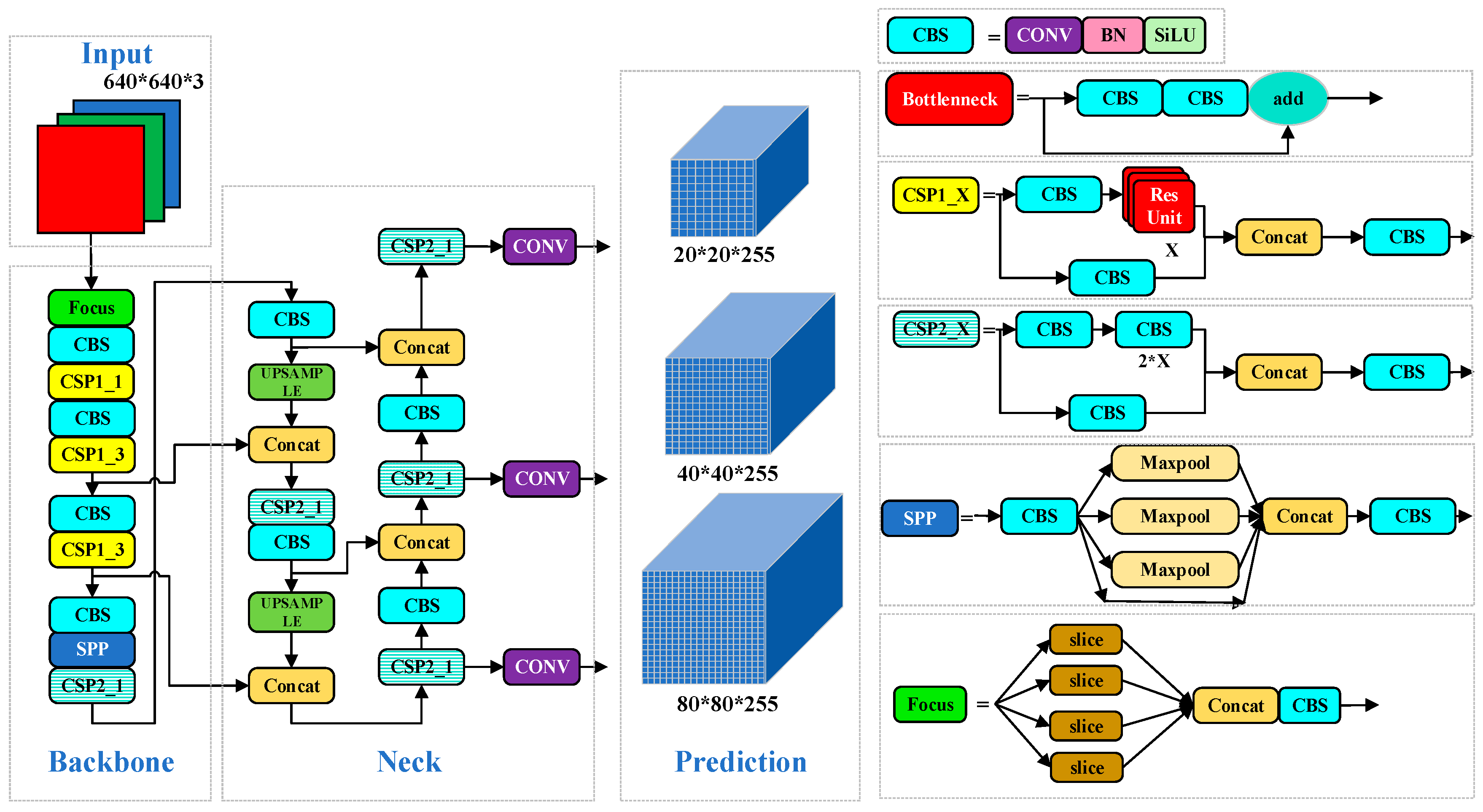
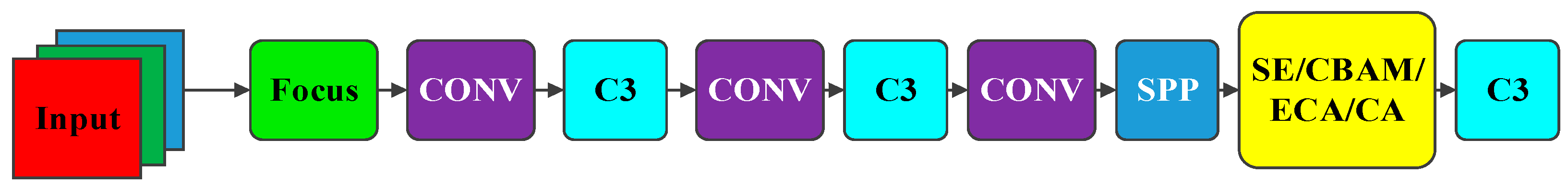
2.4.1. YOLOv5s Structure

In this paper, the default YOLOv5s model was employed to provide a base reference [33]. YOLOv5s is composed of four main parts. The four parts are Input, Backbone, Neck, and Prediction. As shown in Figure 2, the input refers to the inputted infected wood image. Backbone is mainly used for feature extraction of infected wood on images. The role of Neck is to further combine features and pass them to the next layer. The role of Prediction is to identify the final infected wood by its features.

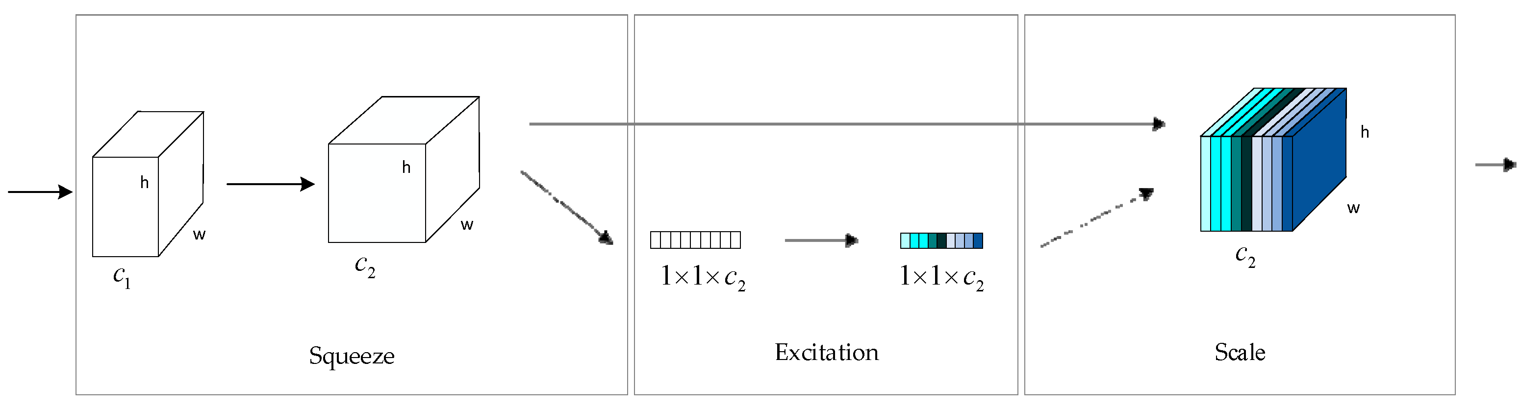
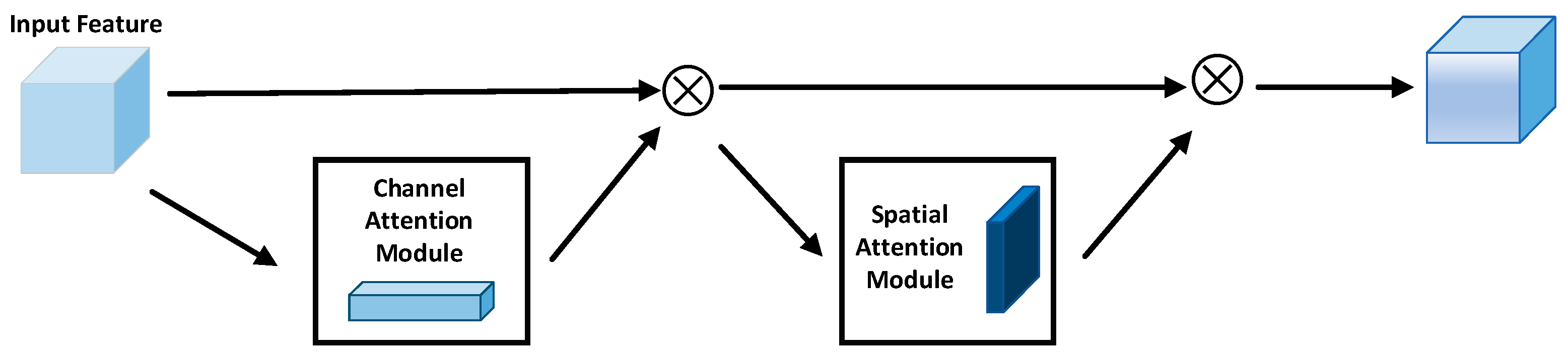
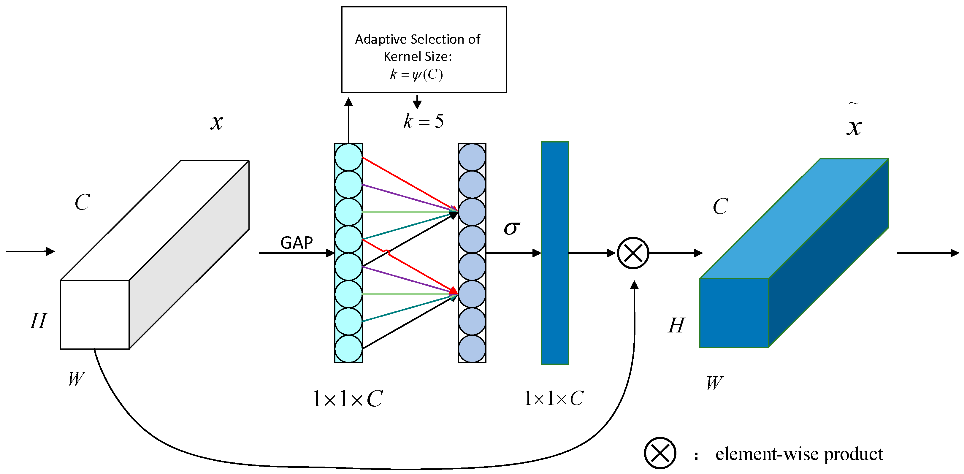
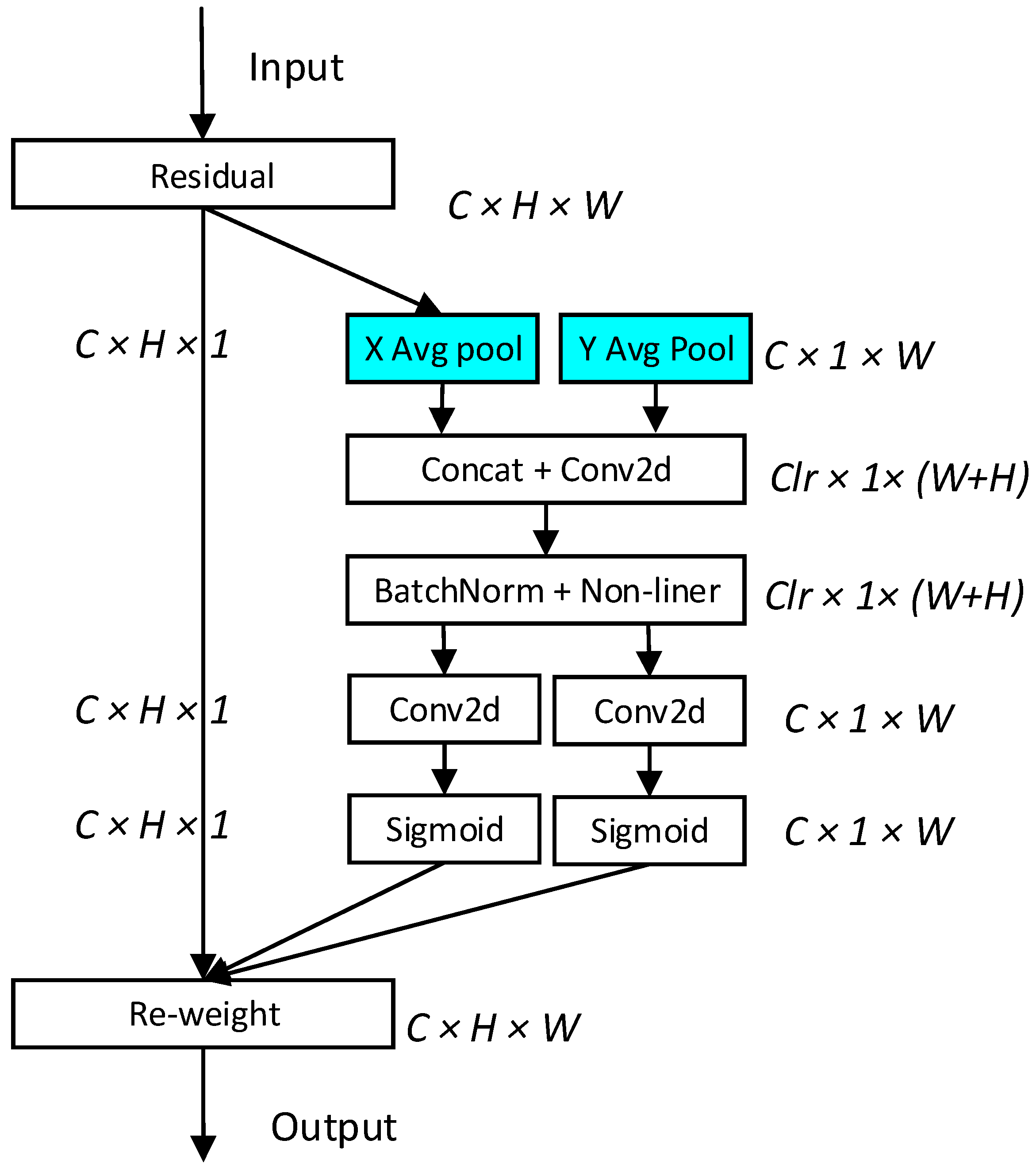
2.4.2. Attention Mechanism

Attention has arguably become one of the most important concepts in the deep learning field. It is inspired by the biological systems of humans that tend to focus on the distinctive parts when processing large amounts of information [35]. In a vision system, an attention mechanism can be treated as a dynamic selection process that is realized by adaptively weighting features according to the importance of the input [36]. The attention mechanism is one of the research directions in machine learning that is attracting more interest recently. It has been shown that attention mechanisms can make improvements compared to the original models. This is because the attention mechanism can improve the generalization ability of machine learning models [35]. However, at this stage, the attention mechanism has been applied less in forestry pest identification. In other fields, such as flame detection [37] and ship detection [38], there is a well of implementation of attention mechanisms. In this work, we tried to apply this mechanism in identifying infected wood caused by PWD.
Based on the experience of our previous studies, different attention mechanisms may have different effects on model improvement. Therefore, this work applied four attention mechanisms to find the most optimal among those mechanisms. These four mechanisms are introduced as the following.
The structure of the SE (squeeze-and-excitation) module is shown in Figure 3. SE consists of two parts, squeeze and excitation [39]. The SE module can emphasize features of interest and highlight the differences between different object features [40]. Lin Y et al. improved the network by inserting SE modules in the deep structure of the network. In this work, the SE model reduced the effect of useless features in the channel that might have a negative impact on recognition accuracy [41].
The structure of CBAM (Convolutional Block Attention Module) is shown in Figure 4. CBAM consists of a Channel Attention Module (CAM) and a Partial Attention Module (SAM) [42]. CAM is mainly used to concentrate important information on the channel dimension. SAM is used to collect important information in the spatial dimension.
The structure of the ECA (Efficient Channel Attention) module is shown in Figure 5. The ECA model is a process of feature enhancement in the channel dimension. The ECA model is designed based on SE models. It fully connects layer to 1×1 convolution that can keep the channel dimension constant while channel attention information is focused [43]. The ECA model improves performance at a lower cost. Usually, the ECA model is used to determine the best location to improve performance [44].
The structure of the CA (Coordinate Attention) module is shown in Figure 6. CA is different from other attention mechanisms. It can capture features on two channels at the same time. This feature helps to improve the focus on target characteristics [45]. Kong L et al. found that adding the CA module could help to extract important feature information without increasing the network parameters and model computation [46].
We expected that the attention mechanism could enhance the extraction of infected wood features. Therefore, four attention mechanisms are used to optimize the original YOLOv5s model. The attention mechanisms were added to the YOLOv5s backbone network. The location of the insert of attention mechanisms is shown in Figure 7 using yellow.
To maximize performance, no changes were made to other modules in the backbone network. Instead, the attention mechanism module was added before the last C3. The focus node was mainly responsible for making slices of inputted images. The convolution (CONV) node consisted of batch normalization (gradient disappearance management) and activation operations. SPP (spatial pyramid pooling) can convert a feature map of arbitrary size into a fixed-size feature vector. C3 was the module that preformed learning on features.

2.5. Implementation and Assessment Methods

2.5.1. Experimental Platform and Parameter Settings

We used a desktop computer with the specifications shown in Table 3. PyTorch1.11.0 (FAIR, Santa Monica, CA and New York, NY, USA) was used as the IDE (Integrated Development Environment). The learning rate was set to 0.01. The Epoch value was set to 300 for the training rounds. The Batch Size was set to 32.
In the table, CPU refers to the central processing unit; GPU refers to the graphics processing unit; CUDA refers to Compute Unified Device Architecture.

2.5.2. Evaluation Indicators

Two evaluation indices, i.e., detection accuracy and detection speed, were used to evaluate the algorithms performance. For the detection accuracy, P (Precision), R (Recall), F1-score, IoU (Intersection of Union), PR curve, AP (Average Precision) and mAP (mean AP) provided us with quantitative metrics for the assessment. For the detection speed, FPS (Frames Per Second) is a widely used indicator.
From those indicators, P is the ratio of the number of correctly predicted positive samples and the number of all predicted positive samples. P is calculated using the following Equation (1):
P r e c i s i o n = T P T P + F P
TP (True positive) refers to the number of positive classes predicted as positive samples FP (False positive) refers to the number of negative classes predicted to be positive samples.
R refers to the ratio of samples with a positive prediction out of all predicted samples. R is calculated using the following Equation (2):
R e c a l l = T P T P + F N
whereas FP refers to the number of negative classes predicted to be positive samples. FN (False Negative) refers to the number of negative samples that were incorrectly predicted by the positive classes.
F1 score is the harmonic mean of P and R. F1 is calculated using the following Equation (3):
F 1   s c o r e = 2 × P × R P + R
whereas P refers to the ratio of the number of correctly predicted positive samples and the number of all predicted positive samples. R refers to the ratio of samples with a positive prediction out of all predicted samples.
Average Precision (AP) indicates the accuracy rate of a class of targets. AP is calculated using the following Equation (4):
A P = 0 1 P ( R ) d R
whereas P refers to the ratio of the number of correctly predicted positive samples and the number of all predicted positive samples; R refers to the ratio of samples with a positive prediction out of all predicted samples.
PR (Precision-Recall) curve is a curve with P as the horizontal coordinate and R as the vertical coordinate. mAP (mean Average Precision) is the average of AP over all detected classes. mAP is calculated using the following Equation (5):
m A P = 1 n i = 1 n A P
whereas AP refers to the accuracy rate of a class of targets.
FPS stands for images per second [47]. Whereas t refers to the time (seconds) that one image is processed. FPS is calculated using the following Equation (6):
F P S = 1 t

3. Results and Discussion

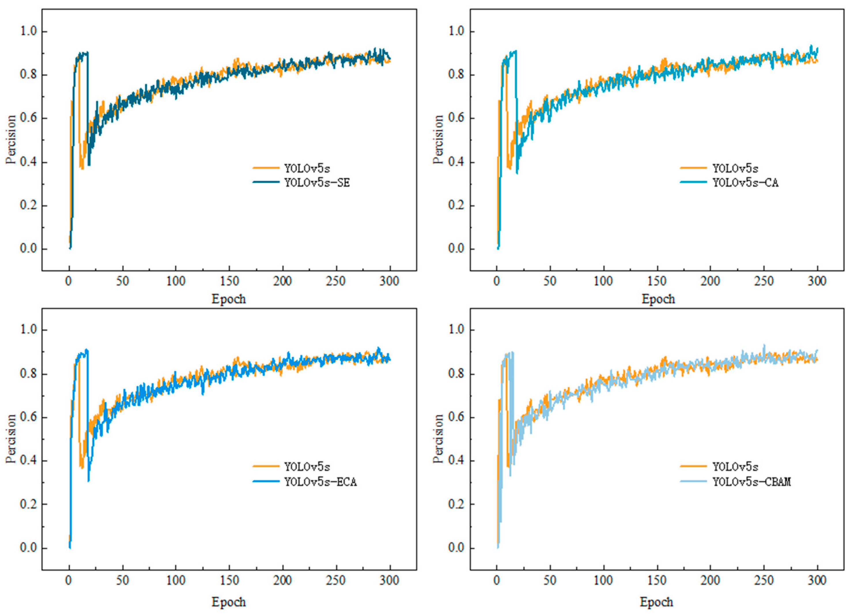
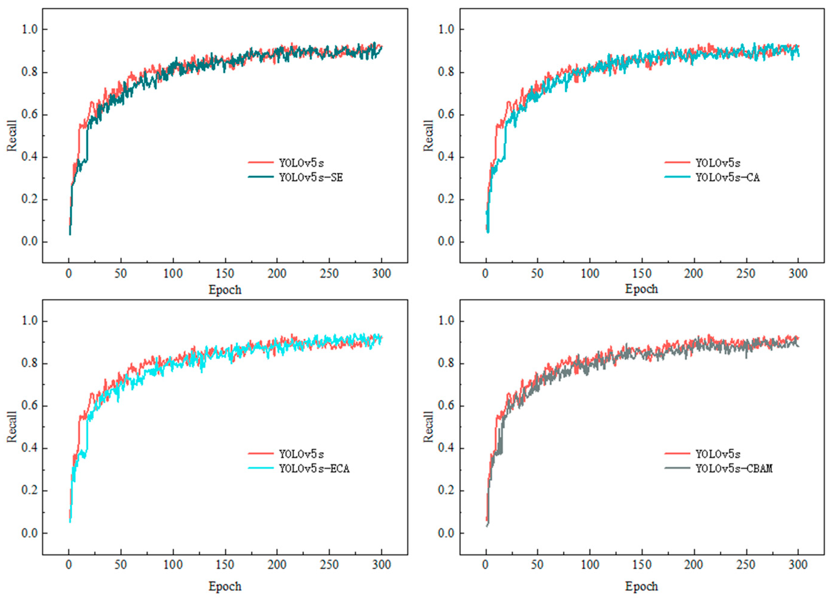
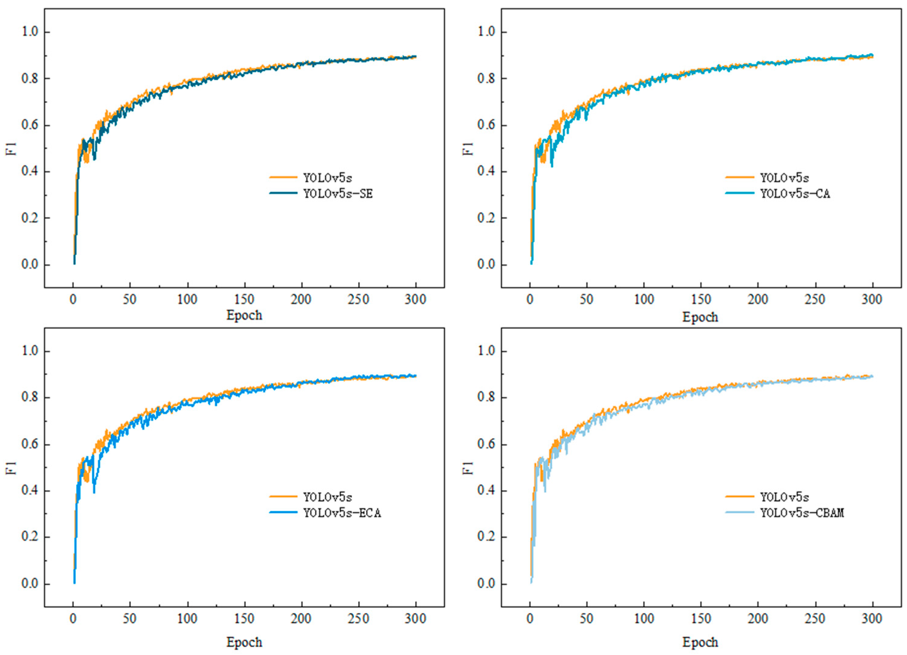
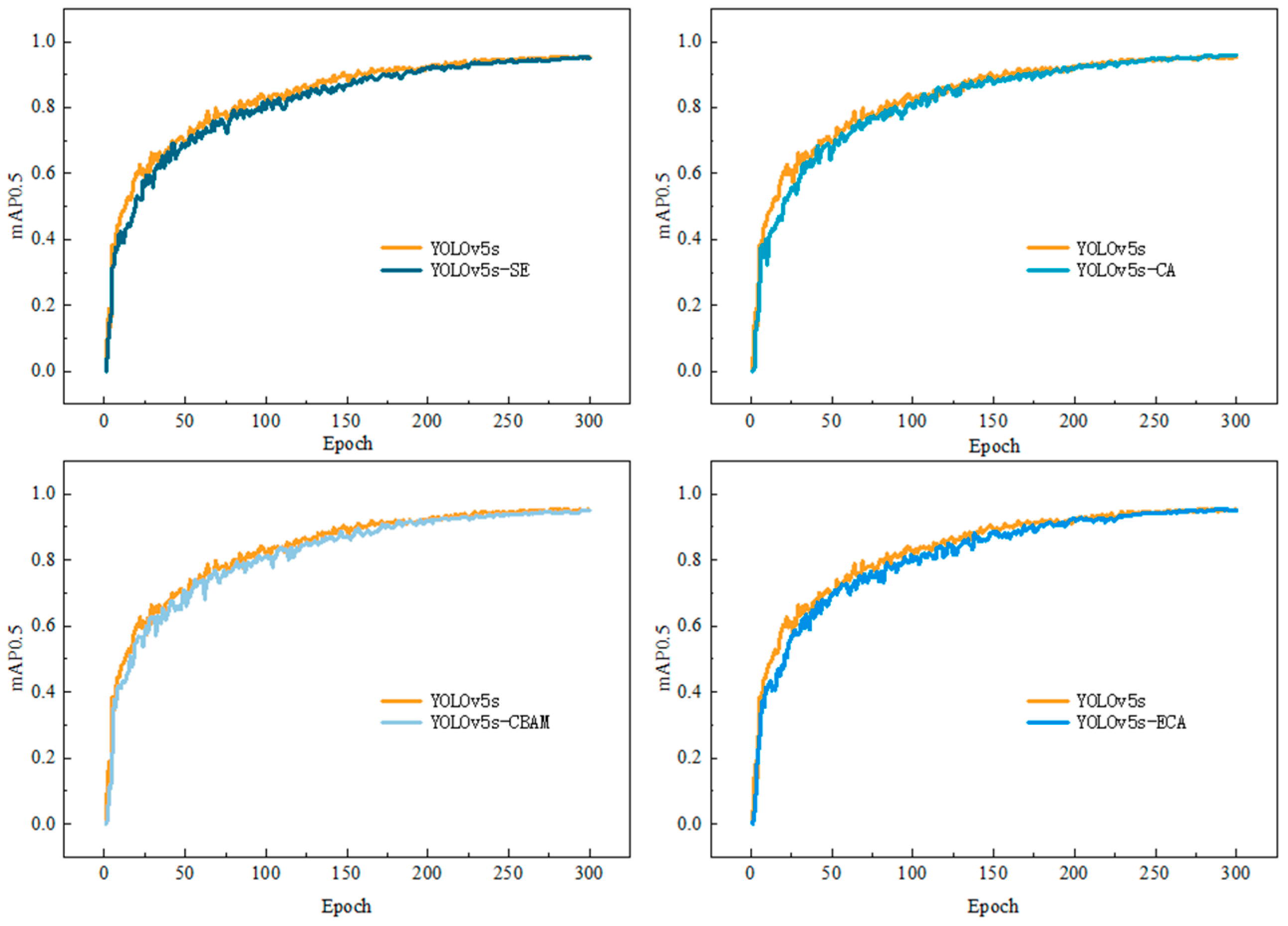
3.1. Training Set Results

Table 4 shows the results of five different models, including the original YOLOv5s, YOLOv5s-SE, YOLOv5s-CA, YOLOv5s-ECA, and YOLOv5s-CBAM. We can see that the precision in the YOLOv5s-ECA model was reduced. Meanwhile, the precision of YOLOv5s-SE, YOLOv5s-CA, and YOLOv5s-CBAM increased compared to the original YOLOv5s model, which indicated that the introduction of attention mechanisms had a notable chance to enhance the overall performance.
For those with positive gains, the YOLOv5s-CA model had the highest accuracy and mAP, which were 95.60% and 97.70%, respectively. YOLOv5s-ECA had the highest recall rate at 95.40%. In terms of file size, the YOLOv5s-CA model weight file is the largest at 16.0 MB. The weight files of YOLOv5s-ECA model and the YOLOv5s were relatively small at ca. 14.4 MB. It could be observed that the addition of attention mechanisms had a minor affect on the file size. It facilitated the re-use of models in different scenarios and multiplatforms.
Figure 8 shows the changes in the accuracy of each model during the training processes. It can be seen that all models had dramatic changes of precision during the initial stage of training. Then the precision gradually increased and stabilized. Among all models, the YOLOv5s-CBAM model used the minimum cycles to become stabilized. The reason could be attributed to the cooperation of both channels in the CBAM model. It accelerated the model training compared to other methods that used one channel. The YOLOv5s-ECA model had the maximum amplitude during the initial stage. This might indicate that the YOLOv5s-ECA model had a faster understanding of the key features of PWD-infected woods.
Figure 9 shows the changes of the recall value of each model during the training processes. The recall value of YOLOv5s-ECA shows notable improvements compared to the original YOLOv5s model. Besides that, no significant differences were found when comparing the models with the attention mechanisms. In the initial rise stage in all figures, we can see that there is a delay of a few rounds between the YOLOv5s model with the attention mechanism and the original YOLOv5s model. The cause for this phenomenon might be related to the added steps imported by attention mechanisms that enhanced the overall complexity.
Figure 10 shows the changes in the F1 score of each model during the training processes. F1 score is a parameter that combines the accuracy and recall, which can be more responsive to the comprehensive performance of the model. In the first 50 rounds of training, the F1 scores of all models improved rapidly and integrated trends of decline. After 50 rounds, F1 scores of all models steadily increased. It indicated that the key features of PWD, such as color and spatial pattern, shown in images were generally identified. The rest of the work would be to improve the overall accuracy.
Figure 11 shows the changes of the mAP value of each model during the training processes. It can be seen that the trend shown in Figure 11 is similar to the one in Figure 9. The high degree of overlap between the trend line of the original YOLOv5s model and the trend line of the modified models decreases the distinguishability of the mAP value.

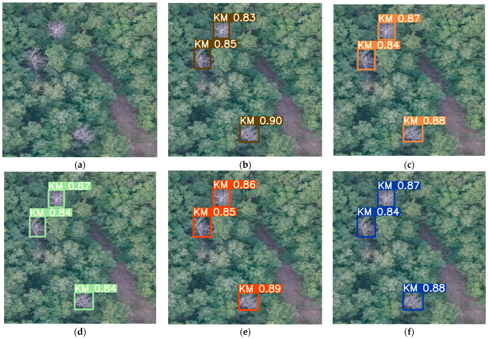
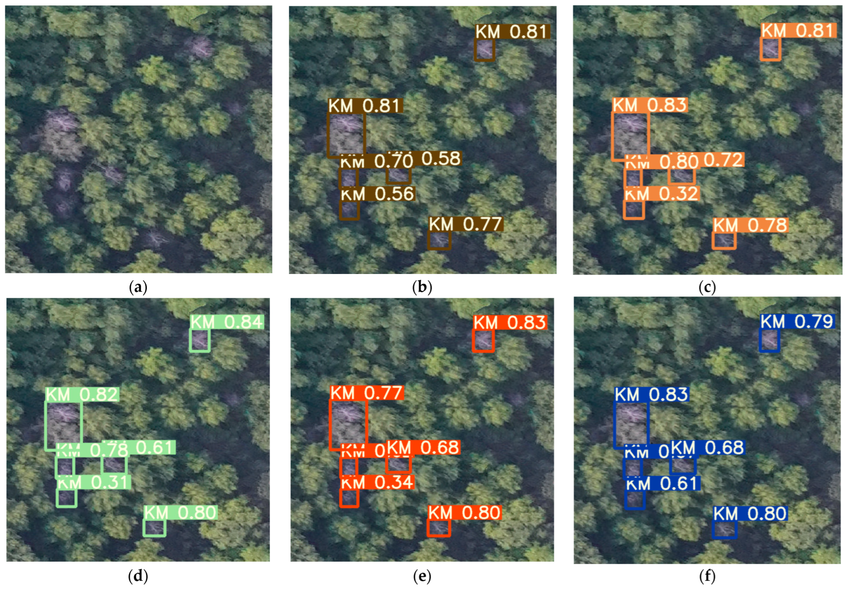
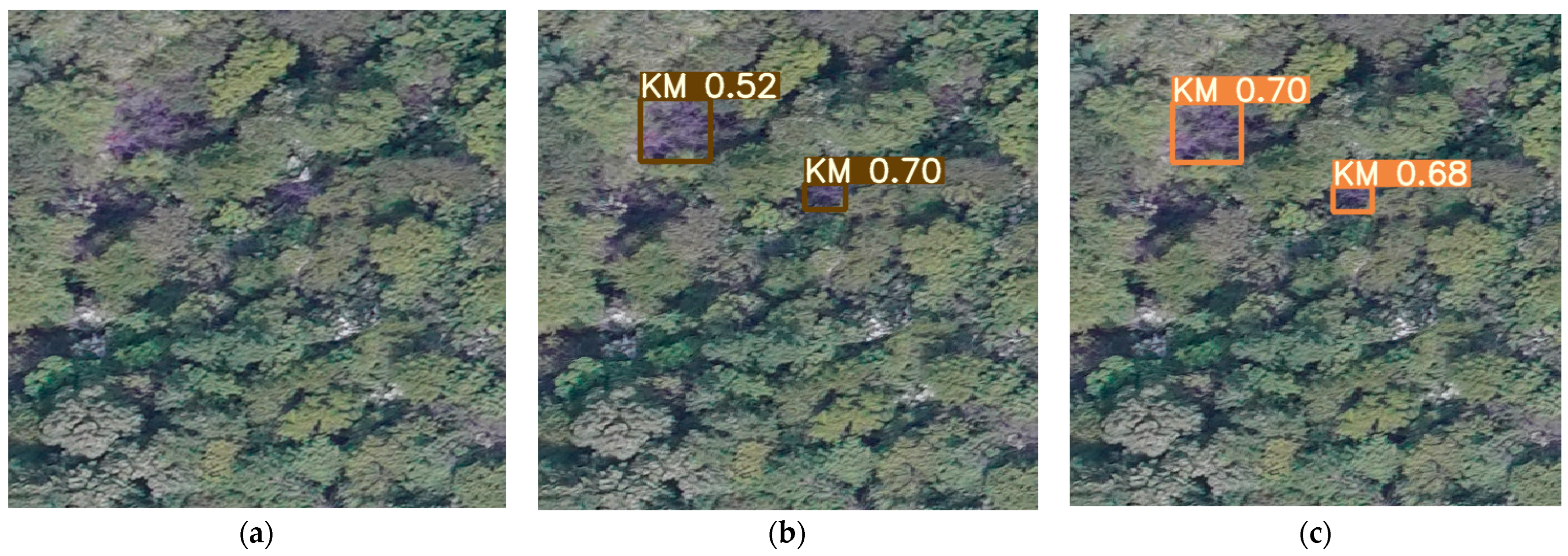
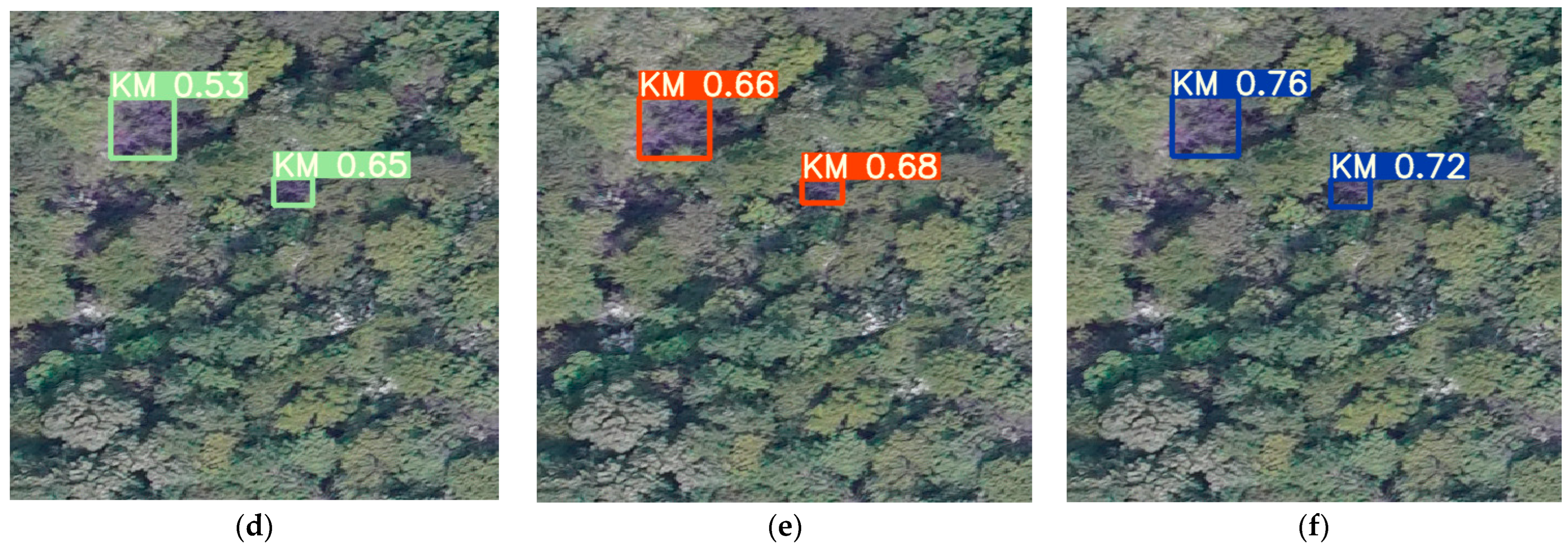
3.2. Test Set Result

Table 5 shows the results of the test set. We can see that the YOLOv5s-ECA model achieved better performance on precision (enhanced by 1.1%) compared to the original YOLOv5s model. On the opposite side, the YOLOv5s-ECA model performed 0.5% worse than the original YOLOv5s model in terms of accuracy on the training set as shown in Table 4. The possible reason could be due to the difference in sample size between the test set and the training set. It is known that the sample size of the training set was 3.5 times larger than the size of the test set. If we input more images into the test set, we would expect that the improvement in accuracy might be reduced to the value of −0.5%. It might be an issue of sample sizes. Due to this finding, we would like to suggest trying to divide the training set and test set in a 1:1 ratio to investigate what would happen in our future work.
Besides the YOLOv5s-ECA model, other models that employed the attention mechanism showed consistency in both the training set and test set. Among them, the YOLOv5s-CA model had the best performance, which was inconsistent with the training set results. Compared to the original YOLOv5s model, the precision of the YOLOv5s-CA model improved at 3.30%. Meanwhile, the average improvement of all models that employed the attention mechanism was 1.30%. For other indicators, for example, the recall value of three models decreased, i.e., the YOLOv5s-SE model, YOLOv5s-CA model, and YOLOv5s-ECA model. The reason was due to the algorithmic features of deep learning methods. It is usual to have different feedback both in precision and recall [48]. For FPS, all models that employed the attention mechanism had improvements compared to the original YOLOv5s. We believe that FPS can also be considered as an indirect indicator to measure the precision. The reason was that a faster model might concentrate key features with high quality together. The possible reason is that a faster model may extract key features with a more concise and effective model.
Figure 12 and Figure 13 show the results of target detection under two typical conditions, i.e., the scatter (Figure 12) and density (Figure 13) distribution of infected wood. In the conditions of the scatter distribution, the degree of confidence for each infected wood was similar. On the contrary, the degree of confidence of each infected wood had great differences in the conditions of the density distribution. For example, the YOLOv5s-SE model, YOLOv5s-ECA model and YOLOv5s-CBAM model were less effective in the identification of infected wood. Meanwhile, YOLOv5s-CA had the most stable performance.
Figure 14 shows the target detection results under the condition of the affected wood pictures which are difficult to judge directly by human eyes. For example, all models can successfully identify the infected wood. YOLOv5s-SE model, YOLOv5s-ECA model and YOLOv5s-CBAM model are less effective in the identification of infected wood. Meanwhile, YOLOv5s-CA had the most stable performance.
We concluded that the possible reasons for why the YOLOv5s-CA model achieved the best performance were the following: The primary cause might be the mechanism of the CA model itself. As mentioned above in Section 2.4.2, the mechanism of the CA model was more focused on helping the main backbone network to extract the features of the infected woods by reducing the unimportant information. Meanwhile, key mechanisms in other attention mechanisms, such as the one in the ECA model, did not have this process. From this, it could be seen that applying an additional filter to clear images before the deep learning process could have contributions to the overall results.
The essential subject in this study was the image, as well as pixels of infected woods. Pixels were stored with spatial information in an image. The location information encoding technics in the CA model reported better performance than other attention mechanisms [49]. To be specific, the SE and ECA were better in processing channel information and had no focus on spatial information. The SE model had a notable loss of raw information through a global pooling layer.
Another advantage of the CA model was that it had a smart strategy to control the redundant loss of information. On the contrary, some attention mechanisms, such as the CBAM model, apply a larger compression ratio in processing. For example, the channel dimension in the CBAM model is usually compressed to 1. As a consequence, much more raw information would be lost. Owing to this problem, the CA model uses 2D (two-dimensions) global pooling to convert a feature tensor to a single feature vector, and coordinate attention divides channel attention into two 1D features encoding processes that aggregate data along the two spatial directions. This operation contributed to the precise label of the position of infected wood.

3.3. Improvements and Deficiencies

Compared to previously reported works, our study achieved improvements in terms of statistical indicators. For example, it had significantly higher detection accuracy com-pared to the improved MobileNetv2-YOLOv4 (86.85%) obtained by Zhengzhi Sun et al. [50], and the unsupervised method with decision fusion (91.35%) proposed by Jianhua Wan et al. [51]. The adding of attention mechanisms had the major contribution to the improvement. In addition to the benefit from novel algorithms, the high quality of UAV images could also contribute to the overall results. Furthermore, we did a full clean of the UAV, including the lens of the camera before each flight. This guarantees the good condition of the hardware. Furthermore, we applied manual inspection of each image. All this additional work enhanced the quality of raw images in our study. Compared to previous reported works using UAVs [52,53], our overall accuracy had a notable improvement.
There are several directions for improvement in this study. First of all, the quantity of raw images could be extended. Due to the limitation of the special aviation controls of UAVs in the capital area, we were unable to fly more. According to this problem, we could employ algorithmic compensation, such as GAN (Generative Adversarial Network) methods [54,55]. This work will be listed in our next stage study. Secondly, it would be possible to try modification in the neck network to seek much more potential [49]. In the end, it would be worth having the experiment of the re-use of the trained model in other devices and a simple field. This will listed in our next steps.

4. Conclusions

In this study, the attention mechanism proved its feasibility by yielding a positive gain to the original YOLOv5s model for the detection of infected wood by PWD. All four attention mechanisms, i.e., Coordinate Attention (CA), Efficient Channel Attention (ECA), Convolutional Block Attention Module (CBAM), and Squeeze-and-Excitation (SE), have improved in terms of detection accuracy. The average improvement is 1.10%. Meanwhile, it was found that the CA model has the greatest enhancement of accuracy at 3.30%. Accordingly, the CA model was determined to be the best model. The accuracy of the CA model in the test set was 95.50%, which was far in excess of reported results in satellite-based research. In addition to accuracy, all attention mechanisms showed better technical performance on FPS. Owing to this fact, we presumed that FPS can be also regarded as an indirect indictor of accuracy.
The causes of the improvements by introducing an attention mechanism is expected to be due to the following: First of all, the attention mechanism can reduce the influence of useless features on model recognition to some extent. This feature can contribute to both performances in accuracy and FPS. Secondly, the attention mechanism can enhance the model’s feature selection of infected wood. That is due to 480. Finally, adding the attention mechanism had a reducing effect on the model file size, which provides convenience for the reuse of trained models in small devices.
The overall framework proposed by this work shows a fast response to the spread of PWD. The devices, i.e., the UAV and RBG camera, are cheap. They will not be a financial burden to small scale operators. Meanwhile, by re-use of trained models, there would be no need for expertise in computer science and forestry. Therefore, it is expected to have an easy implementation in PWD control in Beijing and the North China Plain.

Author Contributions

Data acquisition J.Z. (Jun Zheng), N.Z. and D.W.; Data processing, P.Z., J.Z. (Jianqiao Zhu), Y.F. and X.G.; Model construction P.Z. and Z.W.; Visualization, P.Z.; Writing—original draft, P.Z., Z.W., Y.R. and X.G.; Writing—review and editing, P.Z., Z.W., Y.R. and X.G. All authors have read and agreed to the published version of the manuscript.

Funding

This research was funded by University Natural Science Research Project of Anhui Province (grant number KJ2020A0112), University Natural Science Research Project of Anhui Province (grant number KJ2021ZD0177), National Natural Science Foundation of China (grant number 31901240), University Natural Science Research Project of Anhui Province (grant number 2022AH040125) and Beijing Natural Science Foundation (grant number 8234065, 8232038).

Data Availability Statement

Not applicable.

Conflicts of Interest

The authors declare no conflict of interest.

References

  1. Hao, Z.; Huang, J.; Li, X.; Sun, H.; Fang, G. A multi-point aggregation trend of the outbreak of pine wilt disease in China over the past 20 years. For. Ecol. Manag. 2022, 505, 119890. [Google Scholar] [CrossRef]
  2. Li, M.; Li, H.; Sheng, R.-C.; Sun, H.; Sun, S.-H.; Chen, F.-M. The First Record of Monochamus saltuarius (Coleoptera; Cerambycidae) as Vector of Bursaphelenchus xylophilus and Its New Potential Hosts in China. Insects 2020, 11, 636. [Google Scholar] [CrossRef] [PubMed]
  3. Carrasquinho, I.; Lisboa, A.; Inácio, M.L.; Gonçalves, E. Genetic variation in susceptibility to pine wilt disease of maritime pine (Pinus pinaster Aiton) half-sib families. Ann. For. Sci. 2018, 75, 85. [Google Scholar] [CrossRef] [Green Version]
  4. Dou, G.; Yan, D.-H. Research Progress on Biocontrol of Pine Wilt Disease by Microorganisms. Forests 2022, 13, 1047. [Google Scholar] [CrossRef]
  5. Hu, G.; Yin, C.; Wan, M.; Zhang, Y.; Fang, Y. Recognition of diseased Pinus trees in UAV images using deep learning and AdaBoost classifier. Biosyst. Eng. 2020, 194, 138–151. [Google Scholar] [CrossRef]
  6. Wu, W.; Zhang, Z.; Zheng, L.; Han, C.; Wang, X.; Xu, J.; Wang, X. Research Progress on the Early Monitoring of Pine Wilt Disease Using Hyperspectral Techniques. Sensors 2020, 20, 3729. [Google Scholar] [CrossRef]
  7. Li, M.; Li, H.; Ding, X.; Wang, L.; Wang, X.; Chen, F. The Detection of Pine Wilt Disease: A Literature Review. Int. J. Mol. Sci. 2022, 23, 10797. [Google Scholar] [CrossRef]
  8. Lausch, A.; Borg, E.; Bumberger, J.; Dietrich, P.; Heurich, M.; Huth, A.; Jung, A.; Klenke, R.; Knapp, S.; Mollenhauer, H.; et al. Understanding Forest Health with Remote Sensing, Part III: Requirements for a Scalable Multi-Source Forest Health Monitoring Network Based on Data Science Approaches. Remote Sens. 2018, 10, 1120. [Google Scholar] [CrossRef] [Green Version]
  9. Brovkina, O.; Cienciala, E.; Surovy, P.; Janata, P. Unmanned aerial vehicles (UAV) for assessment of qualitative classification of Norway spruce in temperate forest stands. Geo-Spat. Inf. Sci. 2018, 21, 12–20. [Google Scholar] [CrossRef] [Green Version]
  10. Kuswidiyanto, L.W.; Noh, H.H.; Han, X.Z. Plant Disease Diagnosis Using Deep Learning Based on Aerial Hyperspectral Images: A Review. Remote Sens. 2022, 14, 6031. [Google Scholar] [CrossRef]
  11. Kim, S.-R.; Lee, W.-K.; Lim, C.-H.; Kim, M.; Kafatos, M.C.; Lee, S.-H.; Lee, S.-S. Hyperspectral Analysis of Pine Wilt Disease to Determine an Optimal Detection Index. Forests 2018, 9, 115. [Google Scholar] [CrossRef] [Green Version]
  12. Lee, J.B.; Kim, E.S.; Lee, S.H. An Analysis of Spectral Pattern for Detecting Pine Wilt Disease Using Ground-Based Hyperspectral Camera. Korean J. Remote Sens. 2014, 30, 665–675. [Google Scholar] [CrossRef] [Green Version]
  13. Sun, C.; Huang, C.; Zhang, H.; Chen, B.; An, F.; Wang, L.; Yun, T. Individual Tree Crown Segmentation and Crown Width Extraction From a Heightmap Derived From Aerial Laser Scanning Data Using a Deep Learning Framework. Front. Plant Sci. 2022, 13. [Google Scholar] [CrossRef]
  14. Tao, H.; Li, C.; Cheng, C.; Jiang, L.; Hu, H. Research Progress on Remote Sensing Monitoring of pine wilt disease. Forest Research. 2020, 33, 172–183. [Google Scholar] [CrossRef]
  15. Zhang, B.; Ye, H.; Lu, W.; Huang, W.; Wu, B.; Hao, Z.; Sun, H. A Spatiotemporal Change Detection Method for Monitoring Pine Wilt Disease in a Complex Landscape Using High-Resolution Remote Sensing Imagery. Remote Sens. 2021, 13, 2083. [Google Scholar] [CrossRef]
  16. Li, X.; Tong, T.; Luo, T.; Wang, J.; Rao, Y.; Li, L.; Jin, D.; Wu, D.; Huang, H. Retrieving the Infected Area of Pine Wilt Disease-Disturbed Pine Forests from Medium-Resolution Satellite Images Using the Stochastic Radiative Transfer Theory. Remote Sens. 2022, 14, 1526. [Google Scholar] [CrossRef]
  17. Wang, J.; Zhao, J.; Sun, H.; Lu, X.; Huang, J.; Wang, S.; Fang, G. Satellite Remote Sensing Identification of Discolored Standing Trees for Pine Wilt Disease Based on Semi-Supervised Deep Learning. Remote Sens. 2022, 14, 5936. [Google Scholar] [CrossRef]
  18. Zhou, H.; Yuan, X.; Zhou, H.; Shen, H.; Ma, L.; Sun, L.; Fang, G.; Sun, H. Surveillance of pine wilt disease by high resolution satellite. J. For. Res. 2022, 33, 1401–1408. [Google Scholar] [CrossRef]
  19. Nevalainen, O.; Honkavaara, E.; Tuominen, S.; Viljanen, N.; Hakala, T.; Yu, X.; Hyyppä, J.; Saari, H.; Pölönen, I.; Imai, N.N.; et al. Individual Tree Detection and Classification with UAV-Based Photogrammetric Point Clouds and Hyperspectral Imaging. Remote Sens. 2017, 9, 185. [Google Scholar] [CrossRef] [Green Version]
  20. Duarte, A.; Borralho, N.; Cabral, P.; Caetano, M. Recent Advances in Forest Insect Pests and Diseases Monitoring Using UAV-Based Data: A Systematic Review. Forests 2022, 13, 911. [Google Scholar] [CrossRef]
  21. Yu, R.; Luo, Y.; Zhou, Q.; Zhang, X.; Wu, D.; Ren, L. Early detection of pine wilt disease using deep learning algorithms and UAV-based multispectral imagery. For. Ecol. Manag. 2021, 497, 119493. [Google Scholar] [CrossRef]
  22. Qin, J.; Wang, B.; Wu, Y.; Lu, Q.; Zhu, H. Identifying Pine Wood Nematode Disease Using UAV Images and Deep Learning Algorithms. Remote Sens. 2021, 13, 162. [Google Scholar] [CrossRef]
  23. Ye, W.; Lao, J.; Liu, Y.; Chang, C.-C.; Zhang, Z.; Li, H.; Zhou, H. Pine pest detection using remote sensing satellite images combined with a multi-scale attention-UNet model. Ecol. Inform. 2022, 72, 101906. [Google Scholar] [CrossRef]
  24. Hu, G.; Wang, T.; Wan, M.; Bao, W.; Zeng, W. UAV remote sensing monitoring of pine forest diseases based on improved Mask R-CNN. Int. J. Remote Sens. 2022, 43, 1274–1305. [Google Scholar] [CrossRef]
  25. Zang, H.; Wang, Y.; Ru, L.; Zhou, M.; Chen, D.; Zhao, Q.; Zhang, J.; Li, G.; Zheng, G. Detection method of wheat spike improved YOLOv5s based on the attention mechanism. Front. Plant Sci. 2022, 13. [Google Scholar] [CrossRef] [PubMed]
  26. Zhu, Y.; Feng, Z.; Lu, J.; Liu, J. Estimation of Forest Biomass in Beijing (China) Using Multisource Remote Sensing and Forest Inventory Data. Forests 2020, 11, 163. [Google Scholar] [CrossRef] [Green Version]
  27. Jo, S.; Lee, B.; Oh, J.; Song, J.; Lee, C.; Kim, S.; Suk, J. Experimental Study of In-Flight Deployment of a Multicopter from a Fixed-Wing UAV. Int. J. Aeronaut. Space Sci. 2019, 20, 697–709. [Google Scholar] [CrossRef]
  28. Eskandari, R.; Mahdianpari, M.; Mohammadimanesh, F.; Salehi, B.; Brisco, B.; Homayouni, S. Meta-analysis of Unmanned Aerial Vehicle (UAV) Imagery for Agro-environmental Monitoring Using Machine Learning and Statistical Models. Remote Sens. 2020, 12, 3511. [Google Scholar] [CrossRef]
  29. Aslahishahri, M.; Stanley, K.G.; Duddu, H.; Shirtliffe, S.; Vail, S.; Stavness, I. Spatial Super Resolution of Real-World Aerial Images for Image-Based Plant Phenotyping. Remote Sens. 2021, 13, 2308. [Google Scholar] [CrossRef]
  30. Zaki, N.H.M.; Chong, W.S.; Muslim, A.M.; Reba, M.N.M.; Hossain, M.S. Assessing optimal UAV-data pre-processing workflows for quality ortho-image generation to support coral reef mapping. Geocarto Int. 2022, 37, 10556–10580. [Google Scholar] [CrossRef]
  31. Wu, H.-T.; Tang, S.; Huang, J.; Shi, Y.-Q. A novel reversible data hiding method with image contrast enhancement. Signal Process. Image Commun. 2018, 62, 64–73. [Google Scholar] [CrossRef]
  32. Wang, W.; Wang, H.; Yang, S.; Zhang, X.; Wang, X.; Wang, J.; Lei, J.; Zhang, Z.; Dong, Z. Resolution enhancement in microscopic imaging based on generative adversarial network with unpaired data. Opt. Commun. 2022, 503, 127454. [Google Scholar] [CrossRef]
  33. Jung, H.-K.; Choi, G.-S. Improved YOLOv5: Efficient Object Detection Using Drone Images under Various Conditions. Appl. Sci. 2022, 12, 7255. [Google Scholar] [CrossRef]
  34. Yan, B.; Fan, P.; Lei, X.; Liu, Z.; Yang, F. A Real-Time Apple Targets Detection Method for Picking Robot Based on Improved YOLOv5. Remote Sens. 2021, 13, 1619. [Google Scholar] [CrossRef]
  35. Niu, Z.; Zhong, G.; Yu, H. A review on the attention mechanism of deep learning. Neurocomputing 2021, 452, 48–62. [Google Scholar] [CrossRef]
  36. Guo, M.-H.; Xu, T.-X.; Liu, J.-J.; Liu, Z.-N.; Jiang, P.-T.; Mu, T.-J.; Zhang, S.-H.; Martin, R.R.; Cheng, M.-M.; Hu, S.-M. Attention mechanisms in computer vision: A survey. Comput. Vis. Media 2022, 8, 331–368. [Google Scholar] [CrossRef]
  37. Wang, Y.; Hua, C.; Ding, W.; Wu, R. Real-time detection of flame and smoke using an improved YOLOv4 network. Signal Image Video Process. 2022, 16, 1109–1116. [Google Scholar] [CrossRef]
  38. Xie, F.; Lin, B.; Liu, Y. Research on the Coordinate Attention Mechanism Fuse in a YOLOv5 Deep Learning Detector for the SAR Ship Detection Task. Sensors 2022, 22, 3370. [Google Scholar] [CrossRef]
  39. Hu, J.; Shen, L.; Sun, G. Squeeze-and-Excitation Networks. In Proceedings of the 2018 IEEE/CVF Conference on Computer Vision and Pattern Recognition, Salt Lake City, UT, USA, 18–23 June 2018; pp. 7132–7141. [Google Scholar]
  40. Pan, H.; Shi, Y.; Lei, X.; Wang, Z.; Xin, F. Fast identification model for coal and gangue based on the improved tiny YOLO v3. J. Real-Time Image Process. 2022, 19, 687–701. [Google Scholar] [CrossRef]
  41. Lin, Y.; Cai, R.; Lin, P.; Cheng, S. A detection approach for bundled log ends using K-median clustering and improved YOLOv4-Tiny network. Comput. Electron. Agric. 2022, 194, 106700. [Google Scholar] [CrossRef]
  42. Woo, S.; Park, J.; Lee, J.-Y.; Kweon, I.-S. CBAM: Convolutional Block Attention Module. In Proceedings of the European Conference on Computer Vision, Munich, Germany, 8–14 September 2018. [Google Scholar]
  43. Wang, Q.; Wu, B.; Zhu, P.F.; Li, P.; Zuo, W.; Hu, Q. ECA-Net: Efficient Channel Attention for Deep Convolutional Neural Networks. In Proceedings of the 2020 IEEE/CVF Conference on Computer Vision and Pattern Recognition (CVPR), Seattle, WA, USA, 13–19 June 2020; pp. 11531–11539. [Google Scholar]
  44. Kim, M.; Jeong, J.; Kim, S. ECAP-YOLO: Efficient Channel Attention Pyramid YOLO for Small Object Detection in Aerial Image. Remote Sens. 2021, 13, 4851. [Google Scholar] [CrossRef]
  45. Hou, Q.; Zhou, D.; Feng, J. Coordinate Attention for Efficient Mobile Network Design. In Proceedings of the 2021 IEEE/CVF Conference on Computer Vision and Pattern Recognition (CVPR), Nashville, TN, USA, 20–25 June 2021; pp. 13708–13717. [Google Scholar]
  46. Huang, L.; Huang, W. RD-YOLO: An Effective and Efficient Object Detector for Roadside Perception System. Sensors 2022, 22, 8097. [Google Scholar] [CrossRef] [PubMed]
  47. Kong, L.; Wang, J.; Zhao, P. YOLO-G: A Lightweight Network Model for Improving the Performance of Military Targets Detection. IEEE Access 2022, 10, 55546–55564. [Google Scholar] [CrossRef]
  48. Xiao, Y.; Tian, Z.; Yu, J.; Zhang, Y.; Liu, S.; Du, S.; Lan, X. A review of object detection based on deep learning. Multimed. Tools Appl. 2020, 79, 23729–23791. [Google Scholar] [CrossRef]
  49. Du, F.-J.; Jiao, S.-J. Improvement of Lightweight Convolutional Neural Network Model Based on YOLO Algorithm and Its Research in Pavement Defect Detection. Sensors 2022, 22, 3537. [Google Scholar] [CrossRef] [PubMed]
  50. Sun, Z.; Ibrayim, M.; Hamdulla, A. Detection of Pine Wilt Nematode from Drone Images Using UAV. Sensors 2022, 22, 4704. [Google Scholar] [CrossRef]
  51. Wan, J.; Wu, L.; Zhang, S.; Liu, S.; Xu, M.; Sheng, H.; Cui, J. Monitoring of Discolored Trees Caused by Pine Wilt Disease Based on Unsupervised Learning with Decision Fusion Using UAV Images. Forests 2022, 13, 1884. [Google Scholar] [CrossRef]
  52. Xia, L.; Zhang, R.; Chen, L.; Li, L.; Yi, T.; Wen, Y.; Ding, C.; Xie, C. Evaluation of Deep Learning Segmentation Models for Detection of Pine Wilt Disease in Unmanned Aerial Vehicle Images. Remote Sens. 2021, 13, 3594. [Google Scholar] [CrossRef]
  53. You, J.; Zhang, R.; Lee, J. A Deep Learning-Based Generalized System for Detecting Pine Wilt Disease Using RGB-Based UAV Images. Remote Sens. 2021, 14, 150. [Google Scholar] [CrossRef]
  54. Wang, C.; Xu, C.; Yao, X.; Tao, D. Evolutionary Generative Adversarial Networks. IEEE Trans. Evol. Comput. 2019, 23, 921–934. [Google Scholar] [CrossRef] [Green Version]
  55. Sharma, N.; Sharma, R.; Jindal, N. An Improved Technique for Face Age Progression and Enhanced Super-Resolution with Generative Adversarial Networks. Wirel. Pers. Commun. 2020, 114, 2215–2233. [Google Scholar] [CrossRef]
Figure 1. Location of study area.
Forests 14 00588 g001
Figure 2. YOLOv5s structure [34]. In the figure, focus refers to slicing operation; UPSAMPLE refers to up sampling operation; concat refers to fusion channel; CONV refers to standard convolution; BN refers to batch normalization; SiLU refers to activation function; res unit refers to x residual components; maxpool refers to max pooling; slice refers to each slice operation; add refers to fusion addition.
Forests 14 00588 g002
Figure 3. A squeeze-and-excitation block [39]. c1, h and w refers to the three-dimensions of the image; c2, h, and w refers to the three-dimensions of the feature map; 1 × 1 × c2 refers to the size of the pooled feature map; squeeze refers to global distribution of channel-wise responses and shrinking feature maps through spatial dimensions (w × h); excitation refers to explicit model channel-association and gating mechanism to produce channel-wise weights; scale refers to re-weighting the feature maps.
Forests 14 00588 g003
Figure 4. Convolutional block attention module structure diagram [42].
Forests 14 00588 g004
Figure 5. Diagram of the efficient channel attention (ECA) module [43]. In figure, C, H and W refers to the three-dimensions of the image; GAP refers to global average pooling; 1 × 1 × C refers to the size of the pooled feature map; ECA generates channel weights by performing a fast 1D convolution of size k, where k is adaptively determined via a mapping of channel dimension C.
Forests 14 00588 g005
Figure 6. Coordinate attention block [45]. In the figure, C × H × W refers to the three-dimensions of the image; C × H × 1 refers to the size of the pooled feature map; X Avg Pool and Y Avg Pool refers to the one-dimensional horizontal global pooling and one-dimensional vertical global pooling, respectively; C/r × 1× (W + H) refers to the intermediate feature map that encodes spatial information in both the horizontal direction and the vertical direction; Conv2d refers to the two-dimensional convolution; concat refers to the fusion channel; sigmoid refers to the sigmoid function; BatchNorm refers to the BatchNorm algorithm; non-linear refers to non-linear regression; re-weighting refers to re-weighting efforts.
Forests 14 00588 g006
Figure 7. Backbone structure with the attention mechanism module. In the figure, focus refers to the slicing operation. CONV refers to standard convolution. C3 refers to the CSP bottleneck with three convolutions. SPP refers to spatial pyramid pooling.
Forests 14 00588 g007
Figure 8. The changes of precision value during different models’ training.
Forests 14 00588 g008
Figure 9. The changes of the recall value during different models’ training.
Forests 14 00588 g009
Figure 10. The changes of F1 value during different models’ training.
Forests 14 00588 g010
Figure 11. The changes of mAP value during different models’ training.
Forests 14 00588 g011
Figure 12. Comparison of detection performances of different models in the scatter distribution of infected woods. (a) the original image; (b) YOLOv5s; (c) YOLOv5s-SE; (d) YOLOv5s-ECA; (e) YOLOv5s-CBAM; (f) YOLOv5s-CA.
Forests 14 00588 g012
Figure 13. Comparison of detection performances of different models in a dense distribution of infected woods. (a) the original image; (b) YOLOv5s; (c) YOLOv5s-SE; (d) YOLOv5s-ECA; (e) YOLOv5s-CBAM; (f) YOLOv5s-CA. In the figure, KM refers to infected wood; the value aligned to the detection box refers to the degree of confidence.
Forests 14 00588 g013
Figure 14. Comparison of the detection performances of different models for difficult visual determination of infected woods. (a) the original image; (b) YOLOv5s; (c) YOLOv5s-SE; (d) YOLOv5s-ECA; (e) YOLOv5s-CBAM; (f) YOLOv5s-CA.
Forests 14 00588 g014aForests 14 00588 g014b
Table 1. Statistics of spatial distribution and quantities of infected woods.
Simple Plot LocationArea/km2Infected Wood
Cigou Village 9.45120
Luojiatai Village 13.08 15
Baicaowa Village 9.48 22
Huagou Village 12.52 17
Sanjianfang Village 11.61 19
Zhousigou Village 12.96 220
Zhuanshanzi Village 12.91 50
Total842.05 463
Table 2. Datasets for formal analysis.
SetsNumber of Images
Training set 1004
Verification set 144
Test set287
Table 3. Computational environments.
ItemConfiguration
CPUIntel Core i7-11800H (2.30 GHz)
GPUNVIDIA RTX3050 (3072 CUDA cores)
Operating system Windows 10
Software toolsAnaconda 3 (Continuum Analytics, Austin, TX, USA), CUDA 11.2 (NVIDIA, Santa Clara City, CA, USA), Python 3.8
Table 4. Results of different models using the training set.
Model NamePrecision/%Recall/%mAP/%Size/Mb
YOLOv5s92.7094.7097.4014.4
YOLOv5s-SE93.5095.1097.5015.5
YOLOv5s-CA95.6091.8097.7016.0
YOLOv5s-ECA92.2095.4097.6014.4
YOLOv5s-CBAM94.2093.5097.5015.5
Table 5. Results of different models using the test set.
Model NamePrecision/%Recall/%mAP/%FPS/Hz
YOLOv5s89.3089.20 94.20 96
YOLOv5s-SE92.1084.30 95.5098
YOLOv5s-CA92.6087.80 95.50116
YOLOv5s-ECA90.3088.20 95.30102
YOLOv5s-CBAM91.1089.3095.50 102
Disclaimer/Publisher’s Note: The statements, opinions and data contained in all publications are solely those of the individual author(s) and contributor(s) and not of MDPI and/or the editor(s). MDPI and/or the editor(s) disclaim responsibility for any injury to people or property resulting from any ideas, methods, instructions or products referred to in the content.

