
YOLO-Tea: A Tea Disease Detection Model Improved by YOLOv5


Abstract
:1. Introduction
2. Materials and Methods
2.1. Dataset
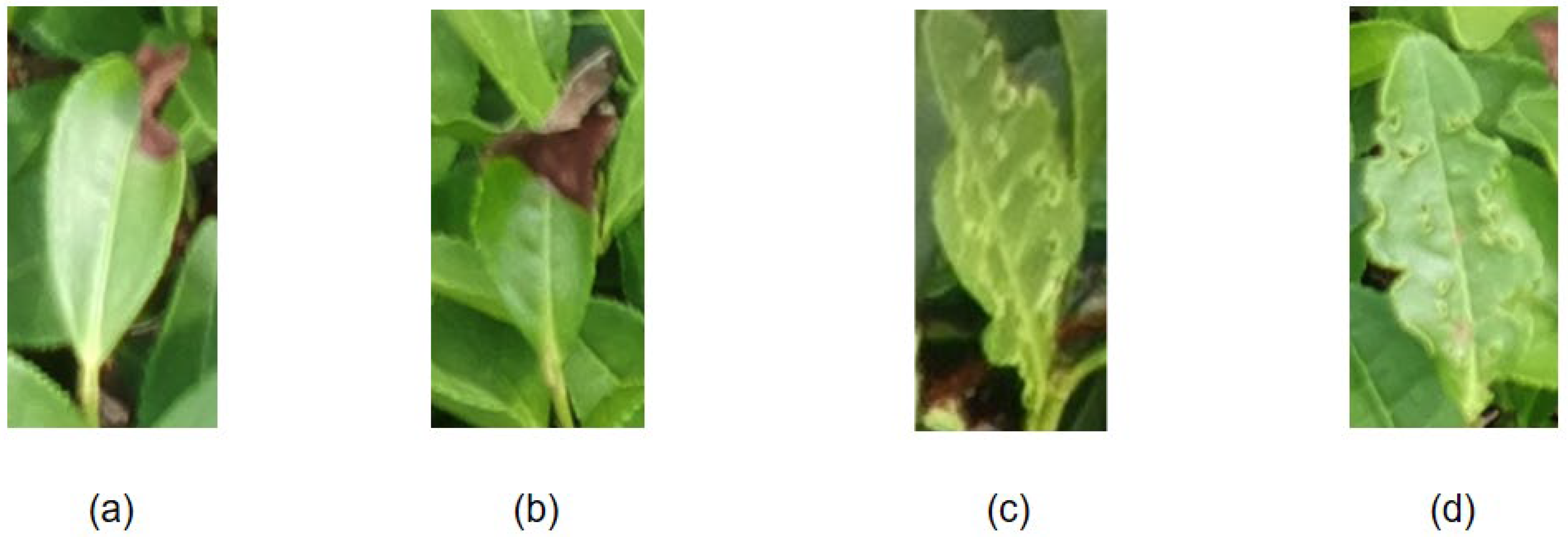
2.1.1. Data Acquisition
2.1.2. Dataset Annotation and Partitioning
2.2. YOLO-Tea
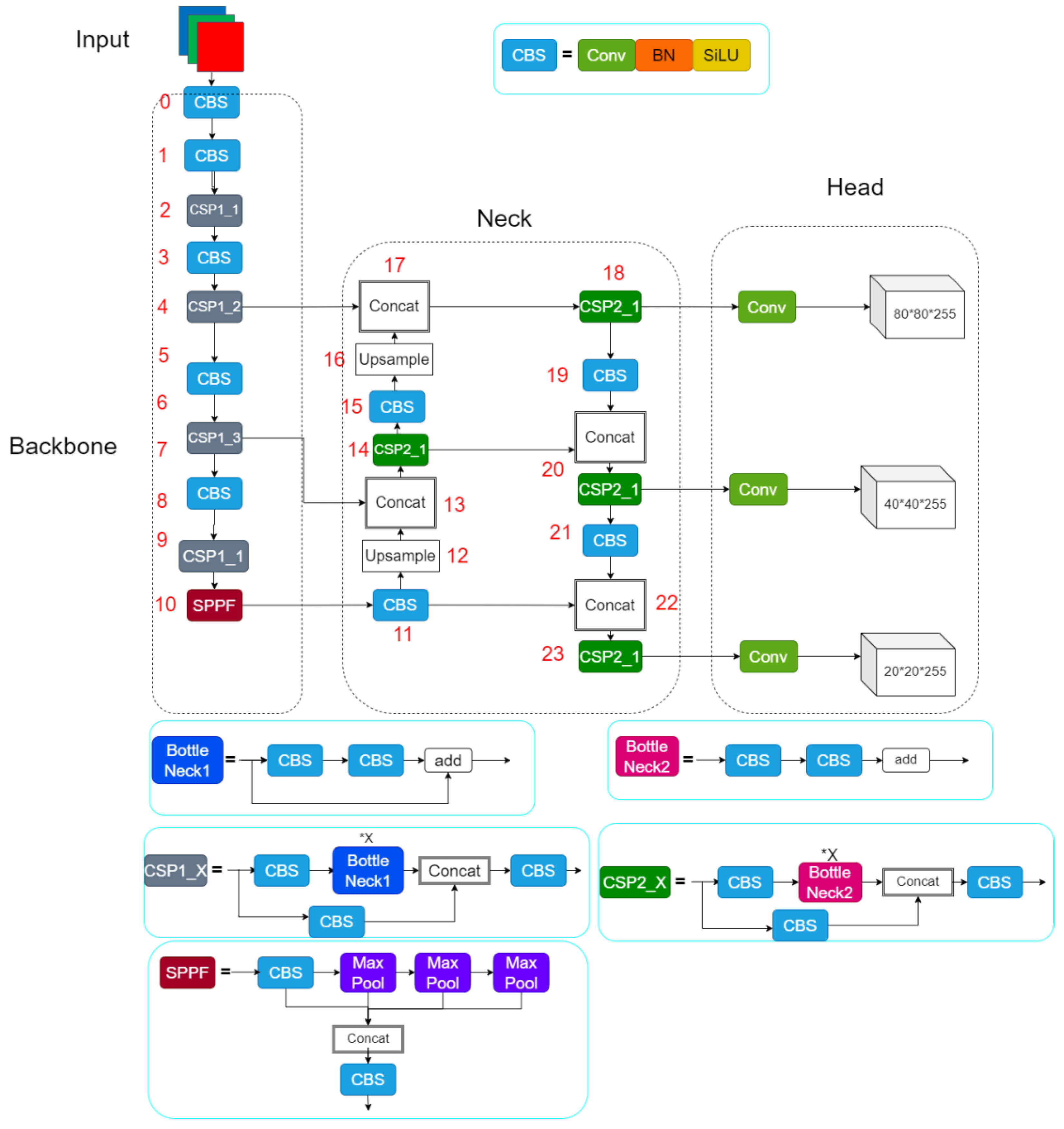
2.2.1. YOLOv5
2.2.2. Convolutional Block Attention Module
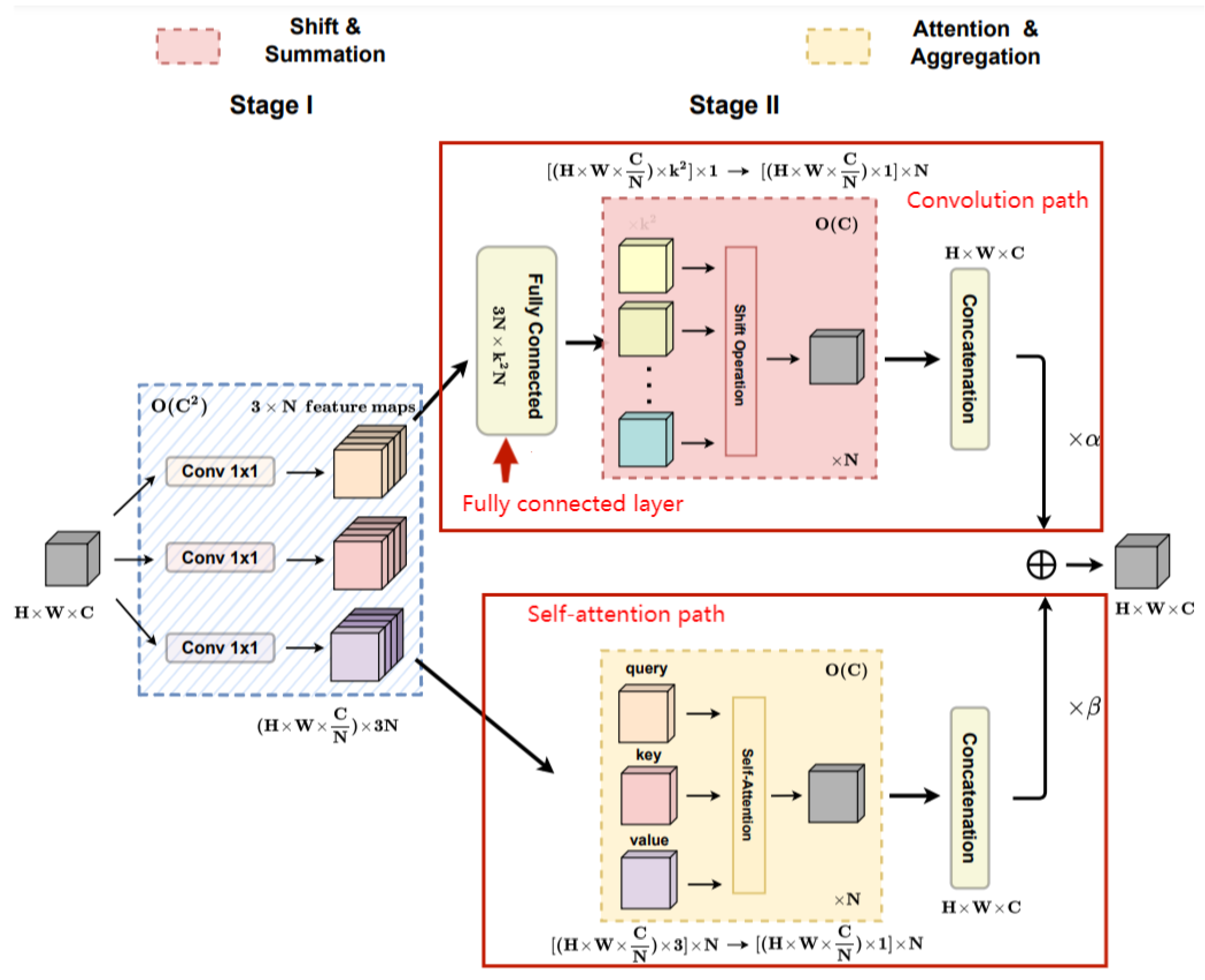
2.2.3. ACmix
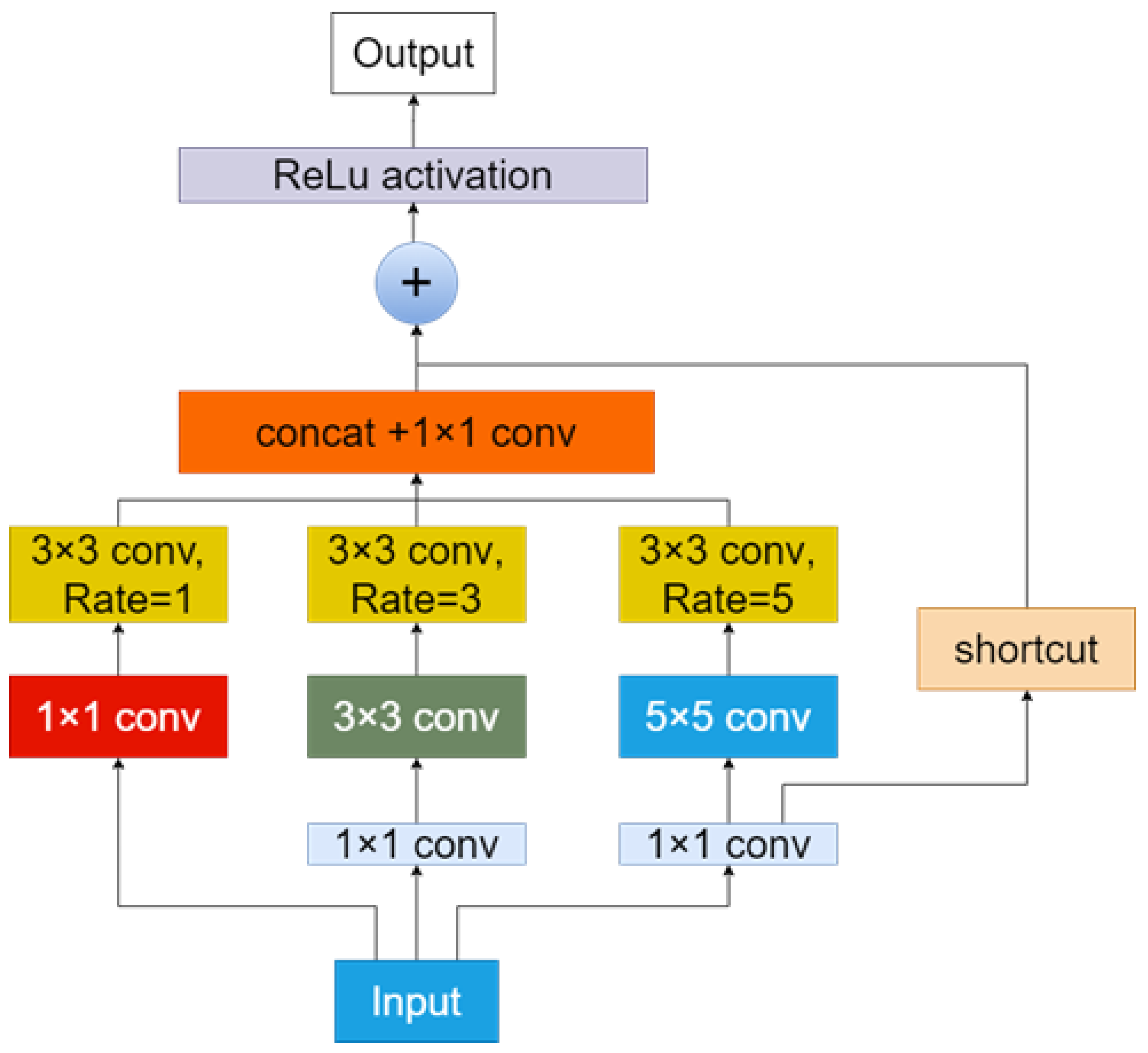
2.2.4. Receptive Field Block
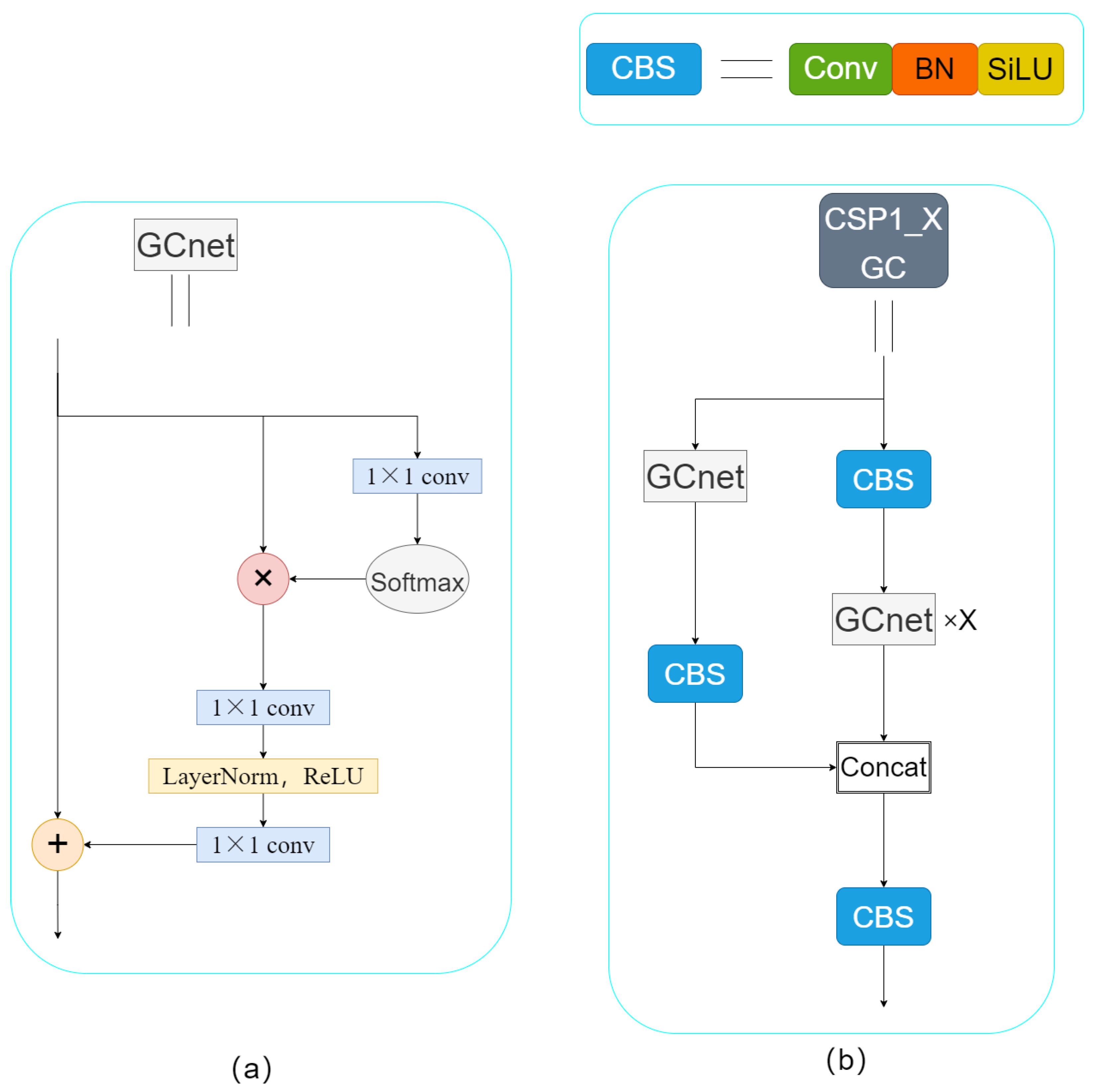
2.2.5. The Methods for Integrating GCNet
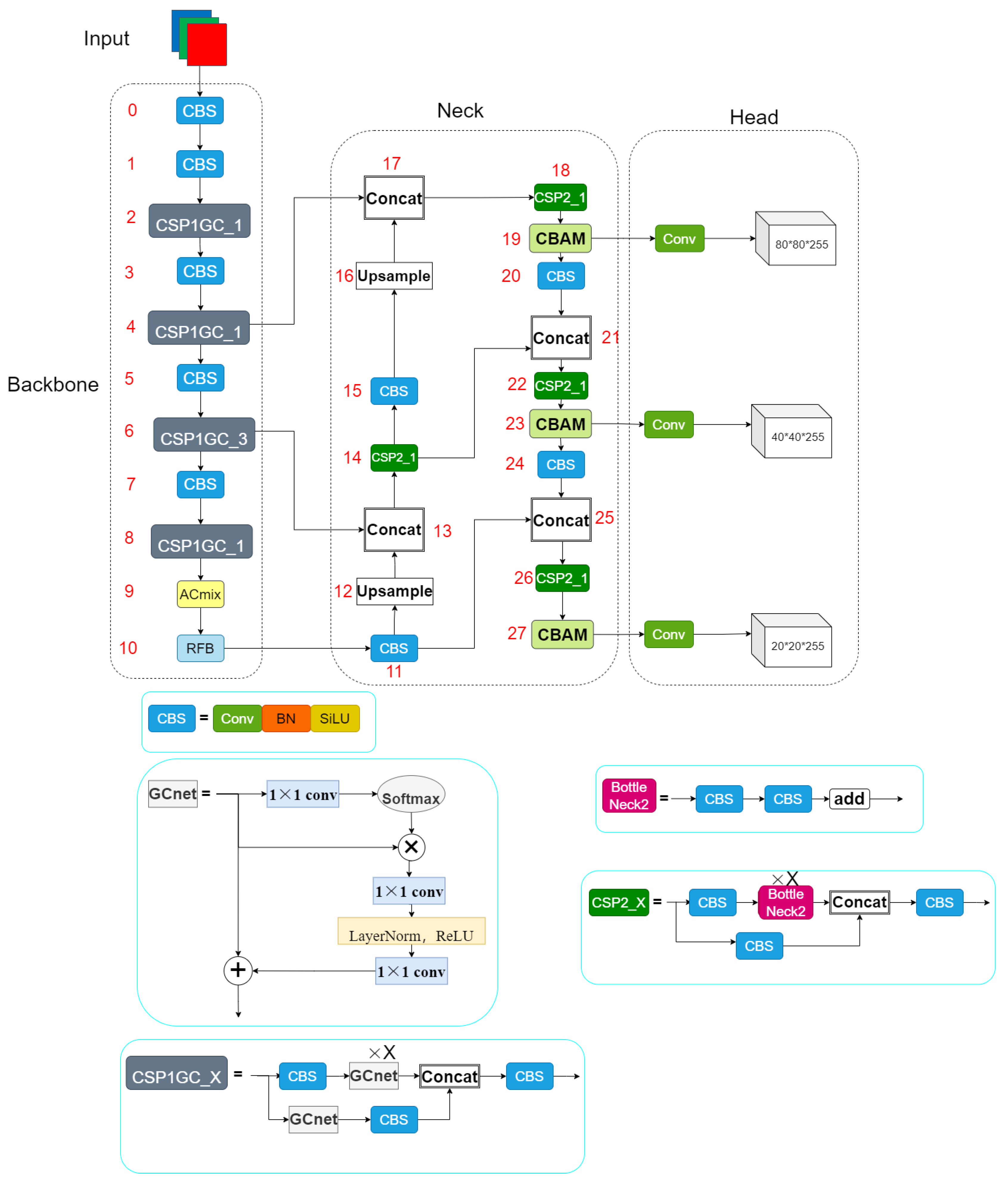
2.2.6. The Structure of YOLO-Tea
2.3. Model Evaluation
3. Results
3.1. Training
3.2. Ablation and Comparison Experiments
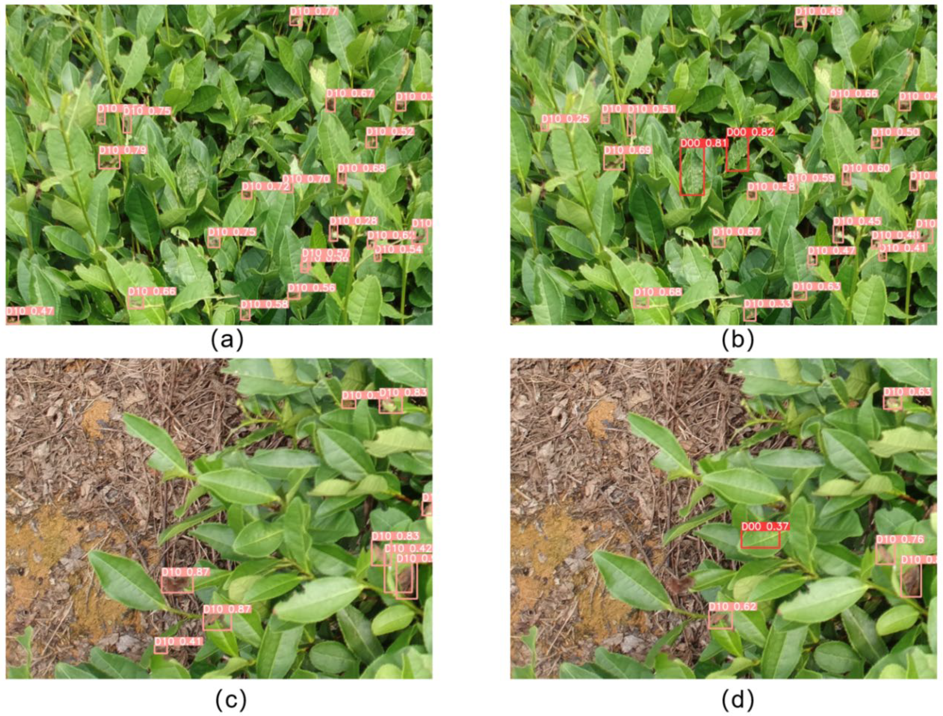
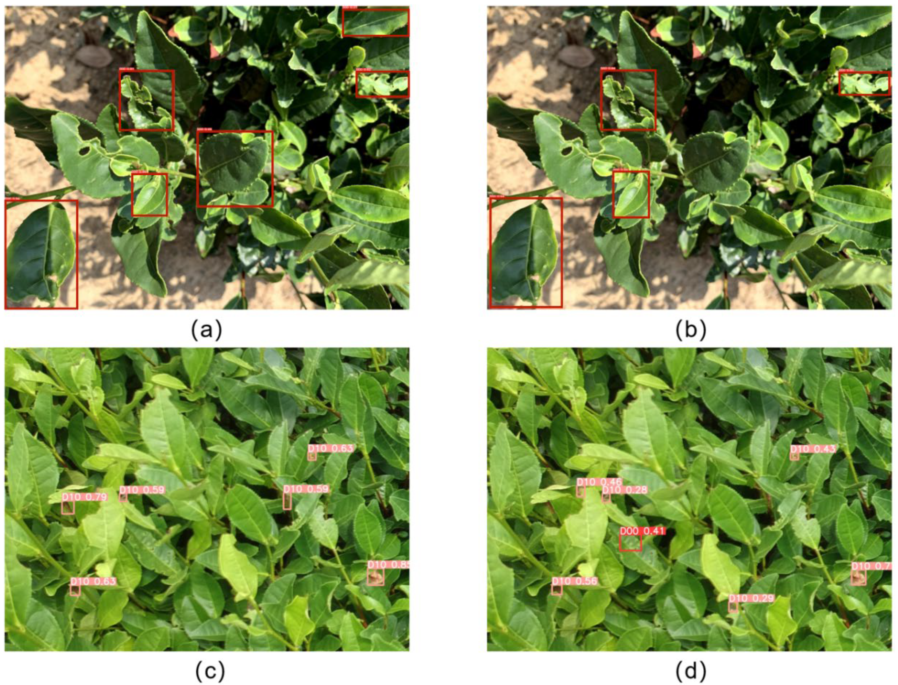
3.3. Comparison
4. Discussion
5. Conclusions
Author Contributions
Funding
Data Availability Statement
Conflicts of Interest
Abbreviations
| CNNs | Convolutional neural networks |
| YOLOv5 | You Only Look Once version 5 |
| CBAM | Convolutional block attention module |
| SPPF | Spatial pyramid pooling fast |
| GCNet | Global context network |
| SLIC | Simple linear iterative cluster |
| SVM | Support vector machine |
| Faster R-CNN | Faster region-based convolutional neural networks |
| SSD | Single Shot Multibox Detector |
| ACmix | Self-attention and convolution |
| CSP1 | Cross-stage partial 1 |
| CSP2 | Cross-stage partial 2 |
| CSPNet | Cross-stage partial networks |
| CAM | Channel attention module |
| SAM | Spatial attention module |
| RFB | Receptive field block |
| SE | Squeeze-and-excitation |
| SNL | Simplified Nonlocal |
| NL | Nonlocal |
| P | Precision |
| R | Recall |
| AP | Average precision |
| IoU | Intersection over union |
| AR | Average recall |
References
- Hu, G.; Yang, X.; Zhang, Y.; Wan, M. Identification of tea leaf diseases by using an improved deep convolutional neural network. Sustain. Comput. Inform. Syst. 2019, 24, 100353. [Google Scholar] [CrossRef]
- Bao, W.; Fan, T.; Hu, G.; Liang, D.; Li, H. Detection and identification of tea leaf diseases based on AX-RetinaNet. Sci. Rep. 2022, 12, 2183. [Google Scholar] [CrossRef] [PubMed]
- Miranda, J.L.; Gerardo, B.D.; Tanguilig, B.T., III. Pest detection and extraction using image processing techniques. Int. J. Comput. Commun. Eng. 2014, 3, 189. [Google Scholar] [CrossRef]
- Barbedo, J.G.A.; Koenigkan, L.V.; Santos, T.T. Identifying multiple plant diseases using digital image processing. Biosyst. Eng. 2016, 147, 104–116. [Google Scholar] [CrossRef]
- Zhang, S.; Wu, X.; You, Z.; Zhang, L. Leaf image-based cucumber disease recognition using sparse representation classification. Comput. Electron. Agric. 2017, 134, 135–141. [Google Scholar] [CrossRef]
- Hossain, S.; Mou, R.M.; Hasan, M.M.; Chakraborty, S.; Razzak, M.A. Recognition and detection of tea leaf’s diseases using support vector machine. In Proceedings of the 2018 IEEE 14th International Colloquium on Signal Processing & Its Applications (CSPA), Penang, Malaysia, 9–10 March 2018. [Google Scholar]
- Sun, Y.; Jiang, Z.; Zhang, L.; Dong, W.; Rao, Y. SLIC_SVM based leaf diseases saliency map extraction of tea plant. Comput. Electron. Agric. 2019, 157, 102–109. [Google Scholar] [CrossRef]
- Chen, J.; Liu, Q.; Gao, L. Visual tea leaf disease recognition using a convolutional neural network model. Symmetry 2019, 11, 343. [Google Scholar] [CrossRef] [Green Version]
- Hu, G.; Wu, H.; Zhang, Y.; Wan, M. A low shot learning method for tea leaf’s disease identification. Comput. Electron. Agric. 2019, 163, 104852. [Google Scholar] [CrossRef]
- Jiang, F.; Lu, Y.; Chen, Y.; Cai, D.; Li, G. Image recognition of four rice leaf diseases based on deep learning and support vector machine. Comput. Electron. Agric. 2020, 179, 105824. [Google Scholar] [CrossRef]
- Sun, X.; Mu, S.; Xu, Y.; Cao, Z.; Su, T. Image recognition of tea leaf diseases based on convolutional neural network. In Proceedings of the 2018 International Conference on Security, Pattern Analysis, and Cybernetics (SPAC), Jinan, China, 14–17 December 2018. [Google Scholar]
- Jiao, L.; Zhang, F.; Liu, F.; Yang, S.; Li, L.; Feng, Z.; Qu, R. A survey of deep learning-based object detection. IEEE Access 2019, 7, 128837–128868. [Google Scholar] [CrossRef]
- Ren, S.; He, K.; Girshick, R.; Sun, J. Faster r-cnn: Towards real-time object detection with region proposal networks. Adv. Neural Inf. Process. Syst. 2015, 28. [Google Scholar] [CrossRef] [Green Version]
- Zhou, G.; Zhang, W.; Chen, A.; He, M.; Ma, X. Rapid detection of rice disease based on FCM-KM and faster R-CNN fusion. IEEE Access 2019, 7, 143190–143206. [Google Scholar] [CrossRef]
- Redmon, J.; Divvala, S.; Girshick, R.; Farhadi, A. You only look once: Unified, real-time object detection. In Proceedings of the IEEE Conference on Computer Vision and Pattern Recognition, Las Vegas, NV, USA, 27–30 June 2016. [Google Scholar]
- Liu, W.; Anguelov, D.; Erhan, D.; Szegedy, C.; Reed, S.; Fu, C.Y.; Berg, A.C. Ssd: Single shot multibox detector. In Proceedings of the European Conference on Computer Vision, Amsterdam, The Netherlands, 11–14 October 2016. [Google Scholar]
- Lin, T.Y.; Goyal, P.; Girshick, R.; He, K.; Dollár, P. Focal loss for dense object detection. In Proceedings of the IEEE International Conference on Computer Vision, Venice, Italy, 22–29 October 2017. [Google Scholar]
- Tian, Y.; Yang, G.; Wang, Z.; Wang, H.; Li, E.; Liang, Z. Apple detection during different growth stages in orchards using the improved YOLO-V3 model. Comput. Electron. Agric. 2019, 157, 417–426. [Google Scholar] [CrossRef]
- Redmon, J.; Farhadi, A. Yolov3: An incremental improvement. arXiv 2018, arXiv:1804.02767. [Google Scholar]
- Roy, A.M.; Bose, R.; Bhaduri, J. A fast accurate fine-grain object detection model based on YOLOv4 deep neural network. Neural Comput. Appl. 2022, 34, 3895–3921. [Google Scholar] [CrossRef]
- Bochkovskiy, A.; Wang, C.; Liao, H.M. Yolov4: Optimal speed and accuracy of object detection. arXiv 2020, arXiv:2004.10934. [Google Scholar]
- Sun, C.; Huang, C.; Zhang, H.; Chen, B.; An, F.; Wang, L.; Yun, T. Individual tree crown segmentation and crown width extraction from a heightmap derived from aerial laser scanning data using a deep learning framework. Front. Plant Sci. 2022, 13, 914974. [Google Scholar] [CrossRef]
- Dai, G.; Fan, J. An industrial-grade solution for crop disease image detection tasks. Front. Plant Sci. 2022, 13, 921057. [Google Scholar] [CrossRef]
- Pan, X.; Ge, C.; Lu, R.; Song, S.; Chen, G.; Huang, Z.; Huang, G. On the integration of self-attention and convolution. In Proceedings of the IEEE/CVF Conference on Computer Vision and Pattern Recognition, New Orleans, LA, USA, 18–24 June 2022. [Google Scholar]
- Woo, S.; Park, J.; Lee, J.Y.; Kweon, I.S. Cbam: Convolutional block attention module. In Proceedings of the European Conference on Computer Vision (ECCV), Munich, Germany, 8–14 September 2018. [Google Scholar]
- Liu, S.; Huang, D. Receptive field block net for accurate and fast object detection. In Proceedings of the European Conference on Computer Vision (ECCV), Munich, Germany, 8–14 September 2018. [Google Scholar]
- Cao, Y.; Xu, J.; Lin, S.; Wei, F.; Hu, H. Gcnet: Non-local networks meet squeeze-excitation networks and beyond. In Proceedings of the IEEE/CVF International Conference on Computer Vision Workshops, Seoul, Republic of Korea, 27–28 October 2019. [Google Scholar]
- Lu, Y.H.; Qiu, F.; Feng, H.Q.; Li, H.B.; Yang, Z.C.; Wyckhuys KA, G.; Wu, K.M. Species composition and seasonal abundance of pestiferous plant bugs (Hemiptera: Miridae) on Bt cotton in China. Crop Prot. 2008, 27, 465–472. [Google Scholar] [CrossRef]
- Qian, J.; Lin, H. A Forest Fire Identification System Based on Weighted Fusion Algorithm. Forests 2022, 13, 1301. [Google Scholar] [CrossRef]
- Wang, C.Y.; Liao HY, M.; Wu, Y.H.; Chen, P.Y.; Hsieh, J.W.; Yeh, I.H. CSPNet: A new backbone that can enhance learning capability of CNN. In Proceedings of the IEEE/CVF Conference on Computer Vision and Pattern Recognition Workshops, Seattle, WA, USA, 14–19 June 2020. [Google Scholar]
- Liu, S.; Qi, L.; Qin, H.; Shi, J.; Jia, J. Path aggregation network for instance segmentation. In Proceedings of the IEEE Conference on Computer Vision and Pattern Recognition, Salt Lake City, UT, USA, 18–23 June 2018. [Google Scholar]
- Wang, X.; Girshick, R.; Gupta, A.; He, K. Non-local neural networks. In Proceedings of the IEEE Conference on Computer Vision and Pattern Recognition, Salt Lake City, UT, USA, 18–23 June 2018. [Google Scholar]
- Hu, J.; Shen, L.; Sun, G. Squeeze-and-excitation networks. In Proceedings of the IEEE Conference on Computer Vision and Pattern Recognition, Salt Lake City, UT, USA, 18–23 June 2018. [Google Scholar]
- Khasawneh, N.; Fraiwan, M.; Fraiwan, L. Detection of K-complexes in EEG signals using deep transfer learning and YOLOv3. Clust. Comput. 2022, 1–11. [Google Scholar] [CrossRef]
- Lin, H.; Tang, C. Intelligent Bus Operation Optimization by Integrating Cases and Data Driven Based on Business Chain and Enhanced Quantum Genetic Algorithm. IEEE Trans. Intell. Transp. Syst. 2021, 23, 9869–9882. [Google Scholar] [CrossRef]
- Lin, H.; Tang, C. Analysis and optimization of urban public transport lines based on multiobjective adaptive particle swarm optimization. IEEE Trans. Intell. Transp. Syst. 2021, 23, 16786–16798. [Google Scholar] [CrossRef]
- Xue, X.; Jin, S.; An, F.; Zhang, H.; Fan, J.; Eichhorn, M.P.; Jin, C.; Chen, B.; Jiang, L.; Yun, T. Shortwave radiation calculation for forest plots using airborne LiDAR data and computer graphics. Plant Phenom. 2022, 2022, 9856739. [Google Scholar] [CrossRef]


| Target | Training Set | Validation Set | Test Set |
|---|---|---|---|
| Green mirid bug (D00) | 1346 | 141 | 177 |
| Tea leaf blight (D10) | 1812 | 192 | 181 |
| Microsoft COCO Evaluation Metrics | |
|---|---|
| Average Precision (AP) | |
| AP at IoU = 0.5 | |
| AP Across Scales | AP at IoU = 0.5:0.95 |
| AP for small target (Size < ) | |
| AP for medium target (< Size < ) | |
| AP for large target (Size > ) | |
| Average Recall (AR) | |
| AR at IoU = 0.5:0.95 | |
| AR Across Scales | |
| AR for small target (Size < ) | |
| AR for medium target (< Size < ) | |
| AR for large target (Size > ) | |
| The metrics we added | |
| AP for tea leaf blight | |
| AP for green mirid bug | |
| Experimental Environment | Details |
|---|---|
| Programming language | Python 3.9 |
| Operating system | Windows 10 |
| Deep learning framework | Pytorch 1.8.2 |
| GPU | NVIDIA GeForce GTX 1070 |
| Training Parameters | Details |
|---|---|
| Epochs | 300 |
| img-size(pixel) | 640 × 640 |
| Initial learning rate | 0.01 |
| Optimization algorithm | SGD |
| Model | ||||||||||
|---|---|---|---|---|---|---|---|---|---|---|
| YOLOv5s (baseline) | 71.7 | 31.1 | 53.6 | 70.1 | 50.2 | 44.6 | 52.6 | 72.1 | 69.3 | 74.1 |
| YOLOv5s + CBAM | 72.4 | 31.4 | 54.4 | 75.3 | 51.6 | 42.2 | 55.4 | 76.1 | 73.3 | 76.3 |
| YOLOv5s + GCnet | 73.0 | 34,2 | 54.6 | 72.4 | 54.0 | 45.4 | 57.5 | 73.3 | 66 | 80.1 |
| YOLOv5 + RFB | 73.7 | 33.1 | 53.9 | 71.2 | 52.4 | 44.9 | 55.4 | 67.5 | 71.2 | 76.1 |
| YOLOv5 + ACmix | 73.7 | 31.2 | 53.8 | 72.1 | 51.1 | 41.7 | 54.9 | 72.4 | 70.6 | 76.8 |
| YOLOv5 + CBAM + ACmix | 75.0 | 33.0 | 54.2 | 79.9 | 52.7 | 39.8 | 58.1 | 80.0 | 71.2 | 78.7 |
| YOLOv5 + CBAM + ACmix + RFB | 75.8 | 32.8 | 56.7 | 82.5 | 54.6 | 44.6 | 58.5 | 84.5 | 71.7 | 79.9 |
| YOLOv5 + CBAM + ACmix + RFB + GCnet (YOLO-Tea) | 79.3 (+7.6) | 34.2 (+3.1) | 57.3 (+3.7) | 85.1 (+15.0) | 54.7 (+4.5) | 44.9 (+0.3) | 57.4 (+4.8) | 85.7 (+13.6) | 73.7 (+4.4) | 82.6 (+8.5) |
| Model | |||
|---|---|---|---|
| YOLOv5s | 71.7 | 69.3 | 74.1 |
| Faster R-CNN | 73.8 | 71.9 | 75.6 |
| SSD | 71.6 | 65.9 | 77.4 |
| YOLO-Tea | 79.3 | 73.7 | 82.6 |
| Model | Parameters | Model Size (MB) |
|---|---|---|
| YOLOv5s | 7025023 | 13.7 |
| YOLOv5s + GCnet | 6262778 | 13.0 (−0.7) |
| YOLOv5 + CBAM + ACmix + RFB | 8722131 | 17.1 |
| YOLO-Tea | 7959886 | 15.6 (−1.5) |
Disclaimer/Publisher’s Note: The statements, opinions and data contained in all publications are solely those of the individual author(s) and contributor(s) and not of MDPI and/or the editor(s). MDPI and/or the editor(s) disclaim responsibility for any injury to people or property resulting from any ideas, methods, instructions or products referred to in the content. |
© 2023 by the authors. Licensee MDPI, Basel, Switzerland. This article is an open access article distributed under the terms and conditions of the Creative Commons Attribution (CC BY) license (https://creativecommons.org/licenses/by/4.0/).
Share and Cite
Xue, Z.; Xu, R.; Bai, D.; Lin, H. YOLO-Tea: A Tea Disease Detection Model Improved by YOLOv5. Forests 2023, 14, 415. https://doi.org/10.3390/f14020415
Xue Z, Xu R, Bai D, Lin H. YOLO-Tea: A Tea Disease Detection Model Improved by YOLOv5. Forests. 2023; 14(2):415. https://doi.org/10.3390/f14020415
Chicago/Turabian StyleXue, Zhenyang, Renjie Xu, Di Bai, and Haifeng Lin. 2023. "YOLO-Tea: A Tea Disease Detection Model Improved by YOLOv5" Forests 14, no. 2: 415. https://doi.org/10.3390/f14020415