

Evaluation of the Ability of SLSTR (Sentinel-3B) and MODIS (Terra) Images to Detect Burned Areas Using Spatial-Temporal Attributes and SVM Classification

 , and
, and
Abstract
:
1. Introduction
2. Materials and Methods
2.1. Materials
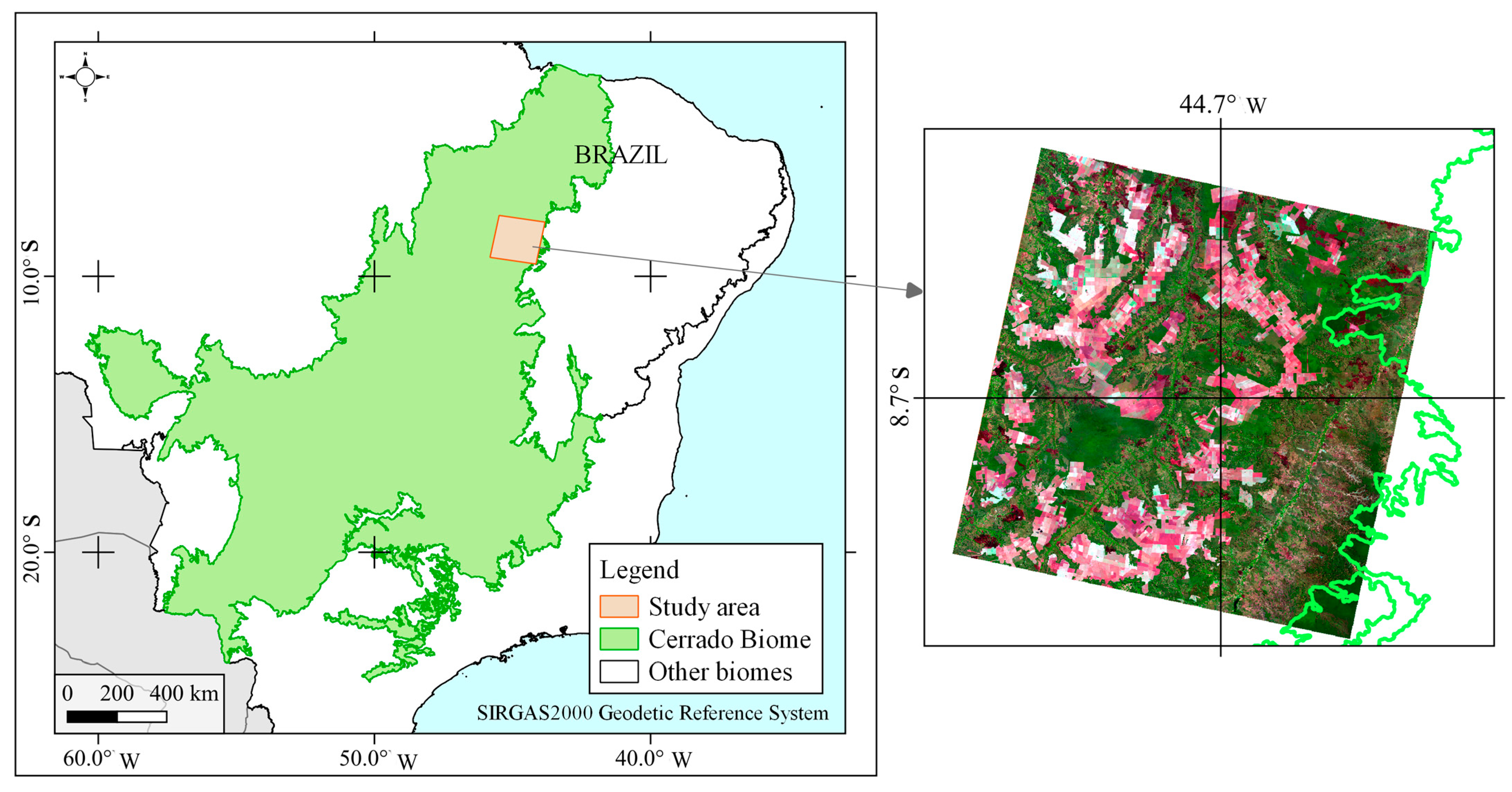
2.1.1. Study Area
2.1.2. Satellite Data
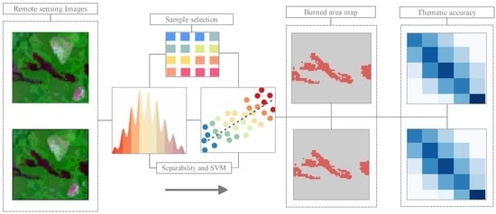
2.2. Methods
2.2.1. Separability Analysis
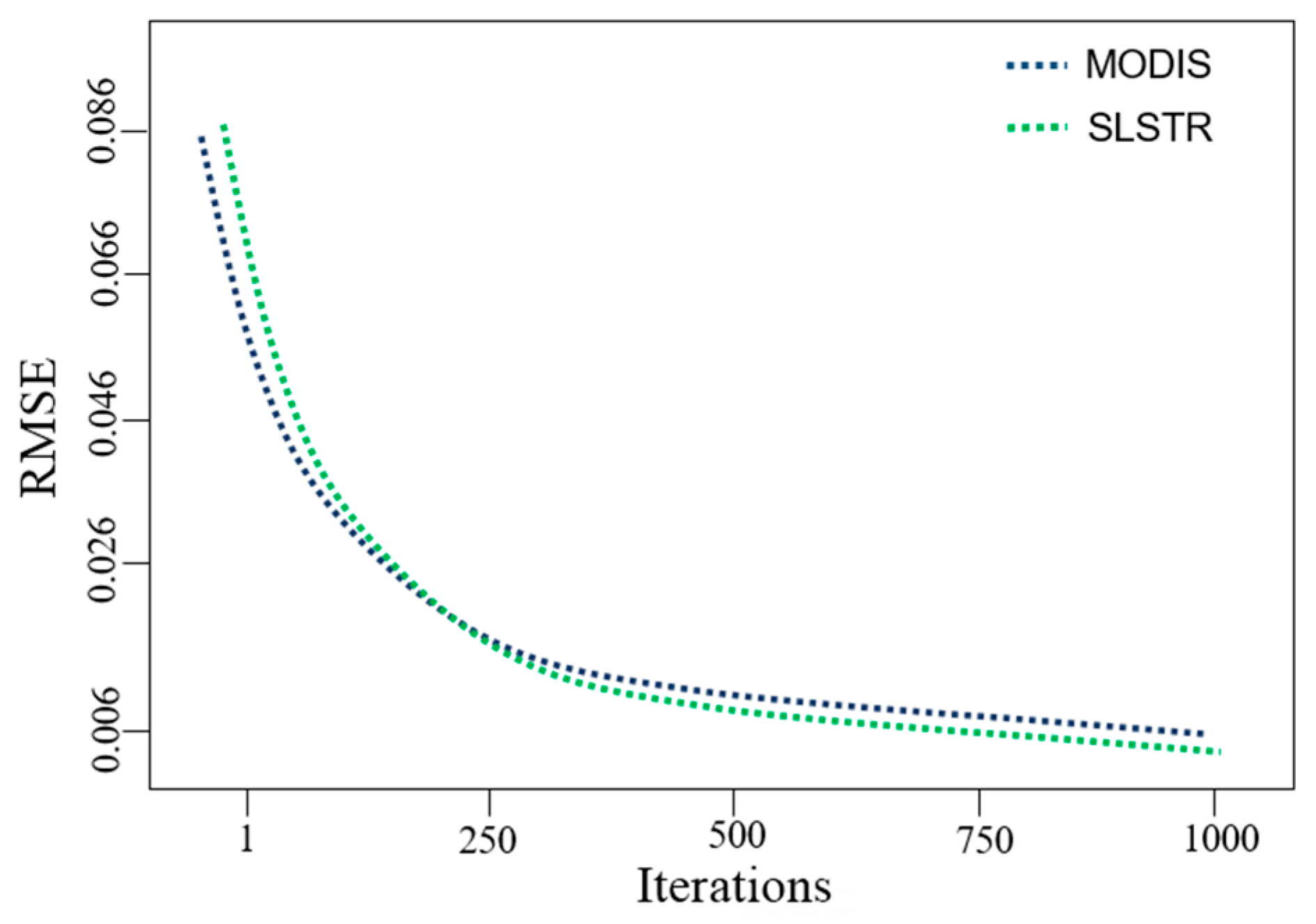
2.2.2. Training and Classification by Support Vector Machine (SVM)
2.2.3. Validation
2.2.4. Accuracy Analysis
2.2.5. Regression Analysis by Proportion of Burned Area in 5 × 5 km Cells
2.2.6. Space-Time Equivalence Coefficient (STEC)
3. Results
3.1. Separability Analysis for SLSTR and MODIS Bands
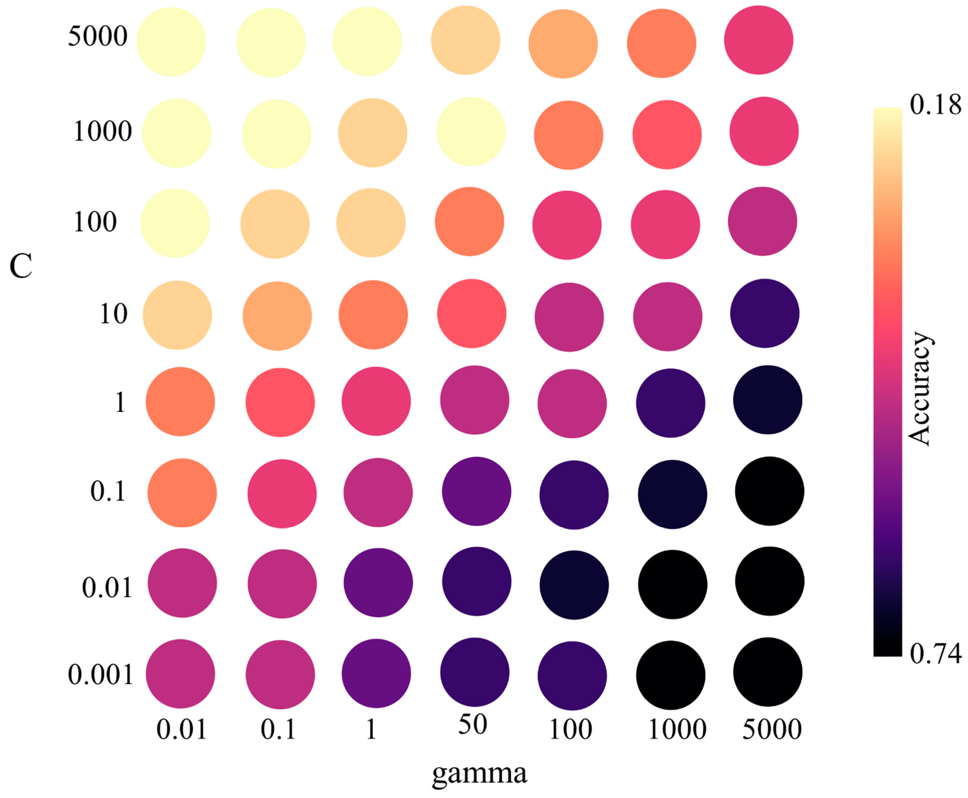
3.2. Effects of Adjustment Parameters on Classification Precision
3.3. SLSTR and MODIS Accuracy Analysis
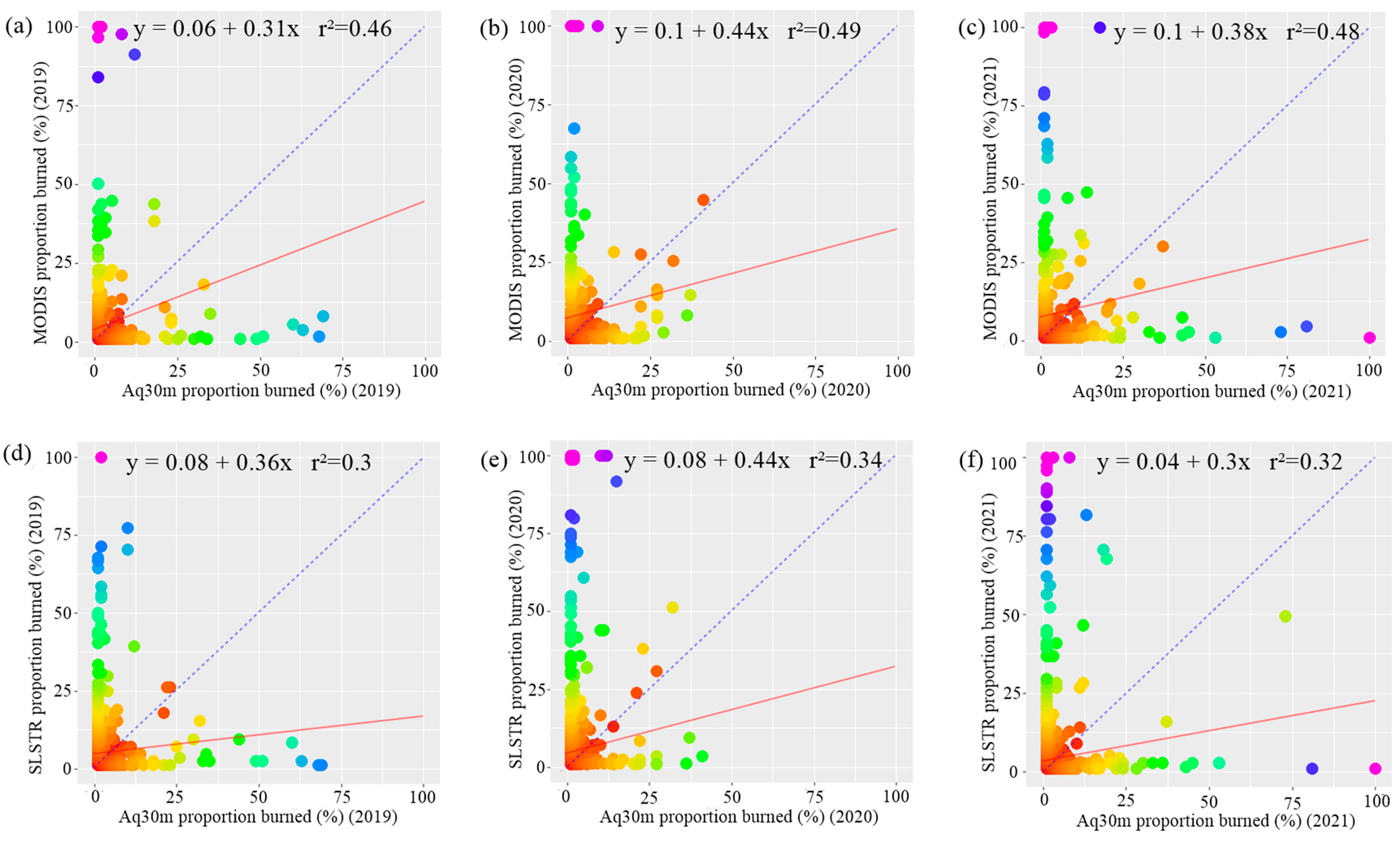
3.4. Proportion of Burned Areas per 5 × 5 km Cells
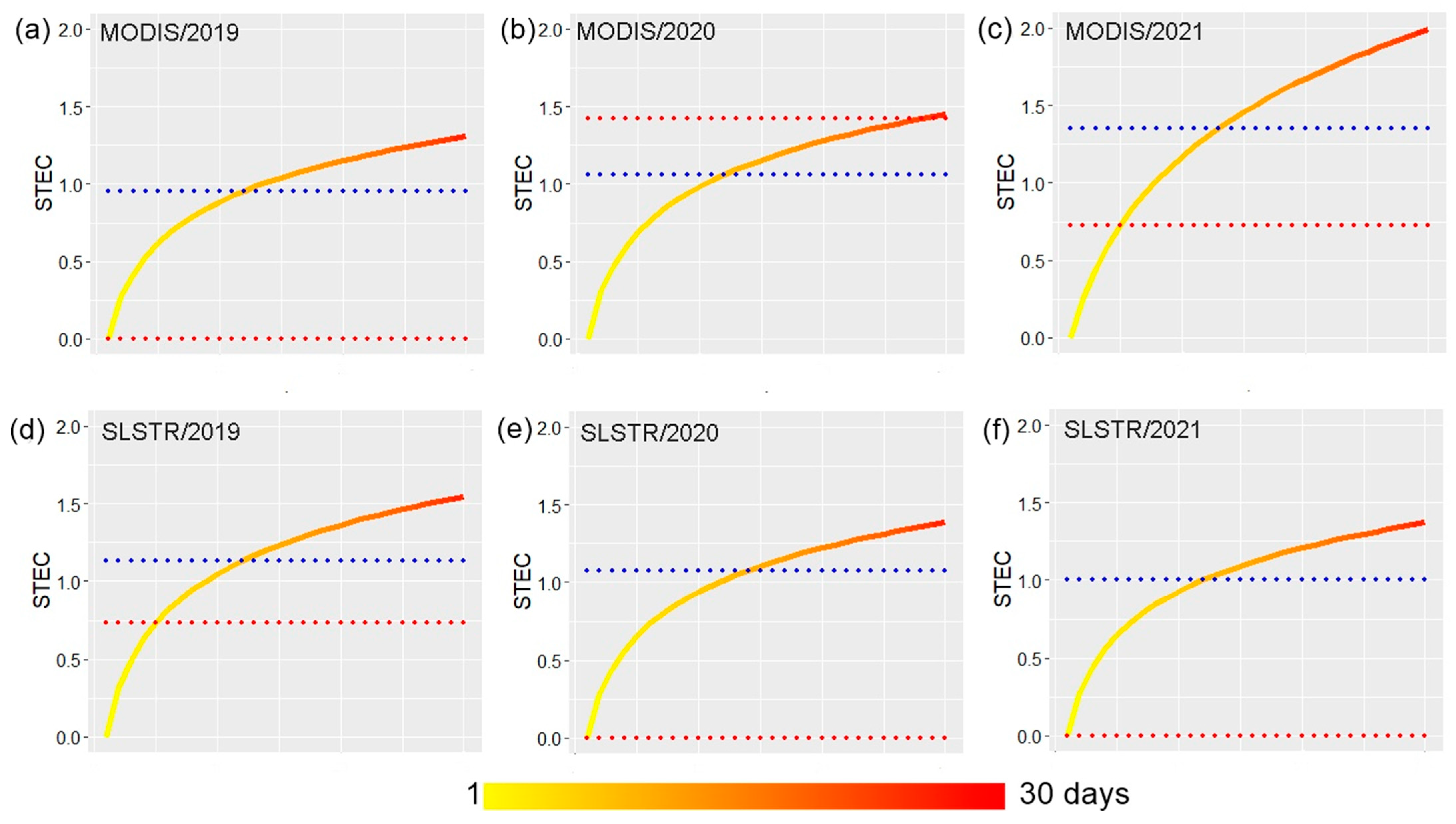
3.5. Assessment of Spatial-Temporal Sensitivity in Fire Detection Based on the STEC Coefficient
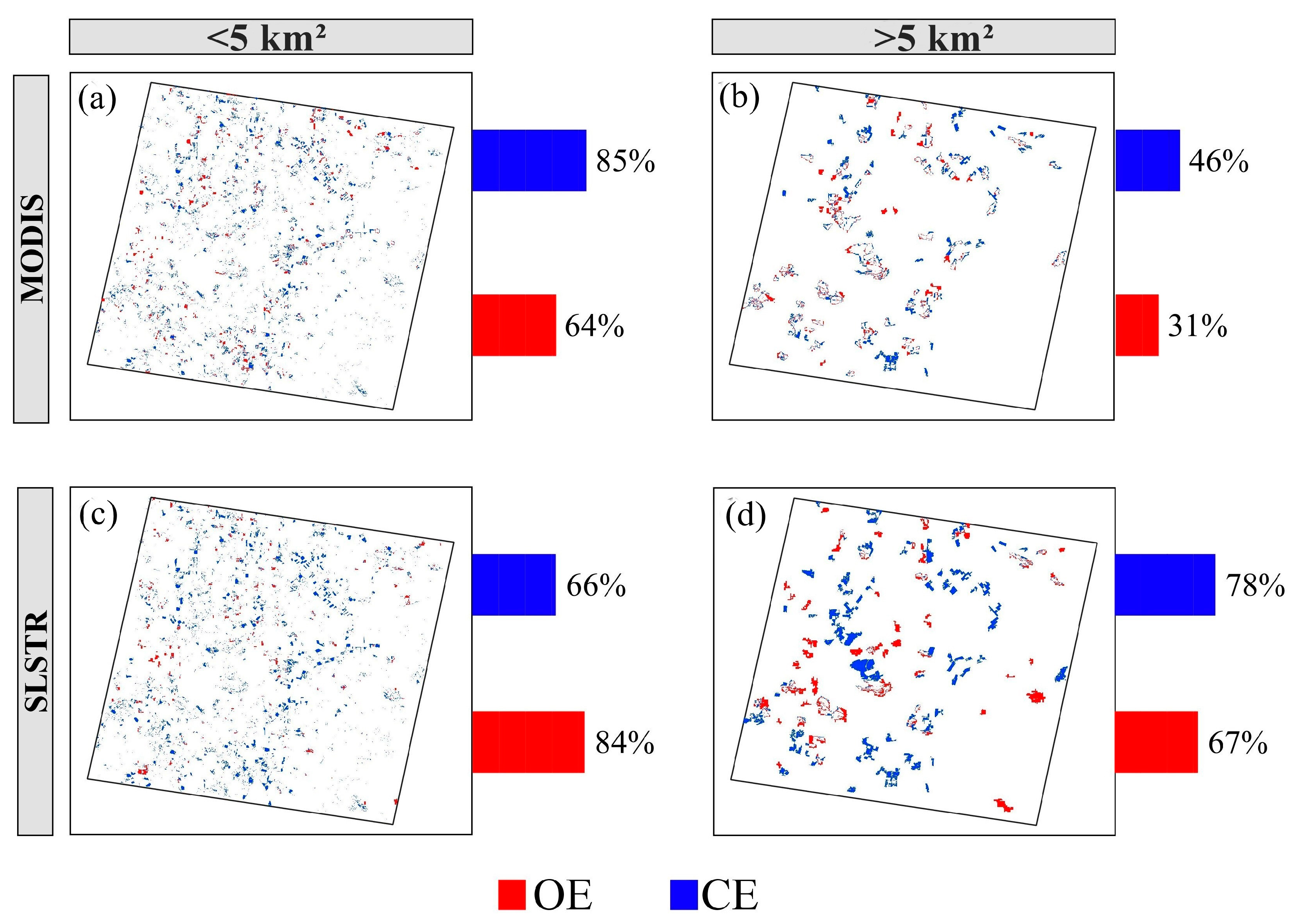
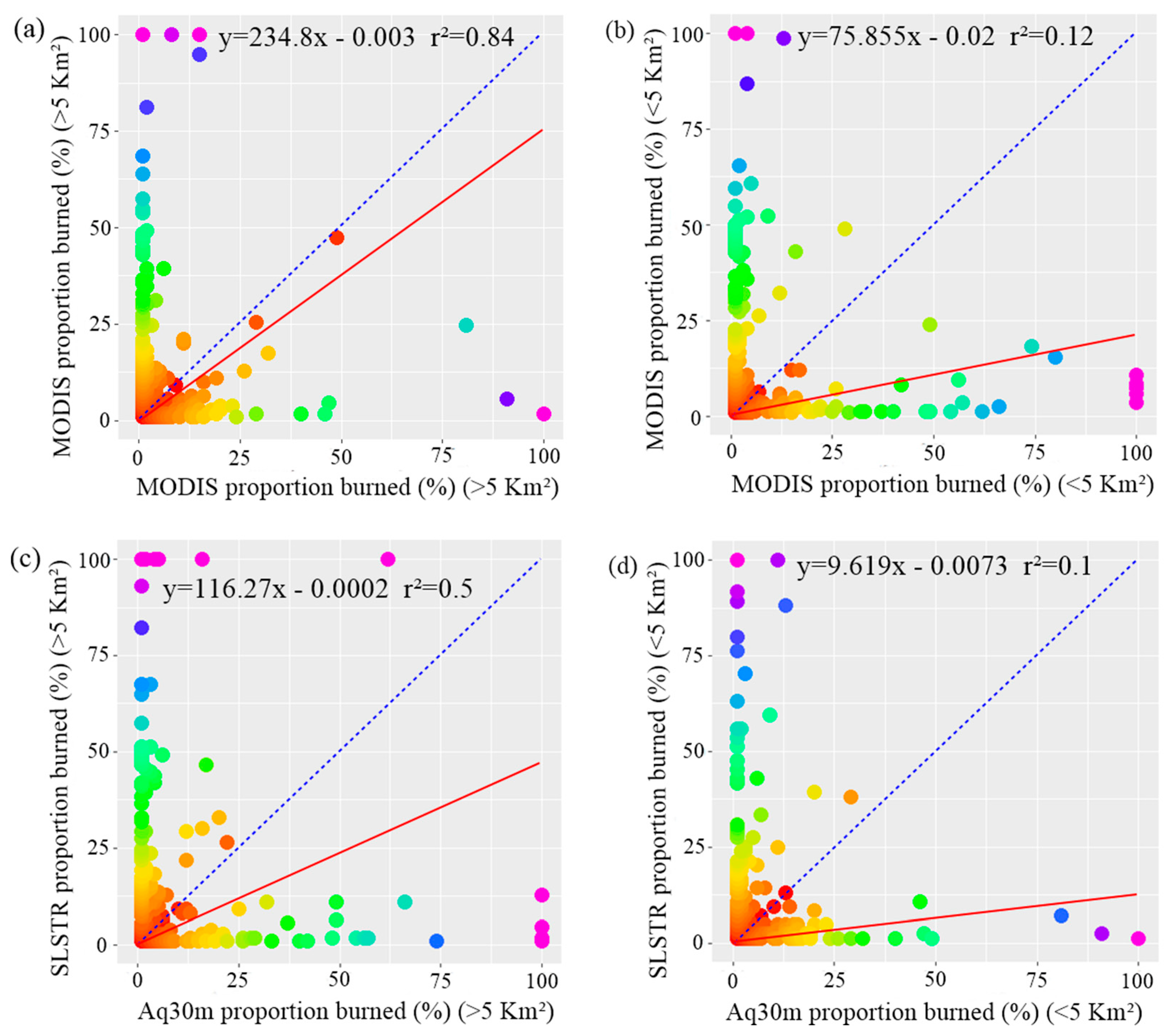
3.6. Analysis of the Accuracy and Linear Regression by Proportion 5 × 5 km for Small and Large Fires in the Year 2021
4. Discussion
4.1. Sensitivity and Separability of Detection Based on Spectral Characteristics
4.2. Analysis of Detection Errors and Relationship with Other Studies in the Mapping of Burned Areas by Satellite
4.3. Influence of Spatial Resolution and Fire Size
4.4. Temporal Influence of Recording of SLSTR and MODIS Scenes Compared to Aq30m
5. Conclusions
Author Contributions
Funding
Data Availability Statement
Conflicts of Interest
References
- Frizzo, T.L.M.; Bonizario, C.; Prado Borges, M.; Vasconcelos, H. Uma revisão dos efeitos do fogo sobre a fauna de formações savânicas do Brasil. Oecologia Aust. 2011, 15, 365–379. Available online: https://revistas.ufrj.br/index.php/oa/article/view/8135 (accessed on 2 November 2021). [CrossRef]
- Reddington, C.L.; Conibear, L.; Robinson, S.; Knote, D.; Arnold, S.R.; Spracklen, D.V. Air Pollution from Forest and Vegetation Fires in Southeast Asia Disproportionately Impacts the Poor. GeoHealth 2021, 5, e2021GH000418. [Google Scholar] [CrossRef]
- Anderson, L.O.; Cheek, D.; EOC Aragao, L.; Andere, L.; Duarte, B.; Salazar, N.; Lima, A.; Duarte, V.; Arai, E. Development of a Point-Based Method for Map Validation and Confidence Interval Estimation: A Case Study of Burned Areas in Amazonia. J. Remote Sens. GIS 2017, 6, 2. [Google Scholar] [CrossRef]
- Redin, M.; dos Santos, G.D.F.; Miguel, P.; Denega, G.L.; Lupatini, M.; Doneda, A.; de Souza, E.L. Impactos Da Queima Sobre Atributos Químicos, Físicos E Biológicos Do Solo. Ciência Florest. 2011, 21, 381–392. [Google Scholar] [CrossRef] [Green Version]
- BRASIL, Ministério do Meio Ambiente. O Bioma Cerrado. 2021. Available online: https://antigo.mma.gov.br/biomas/cerrado.html (accessed on 2 November 2021).
- Lewinsohn, T.M.; Prado, P.I. How Many Species Are There in Brazil? Conserv. Biol. 2005, 19, 619–624. [Google Scholar] [CrossRef]
- Alencar, A.; Shimbo, J.Z.; Lenti, F.; Balzani Marques, C.; Zimbres, B.; Rosa, M.; Arruda, V.; Castro, I.; Ribeiro, J.P.F.M.; Varela, V.; et al. Mapping Three Decades of Changes in the Brazilian Savanna Native Vegetation Using Landsat Data Processed in the Google Earth Engine Platform. Remote Sens. 2020, 12, 924. [Google Scholar] [CrossRef] [Green Version]
- Strassburg, B.B.N.; Brooks, T.; Feltran-Barbieri, R.; Iribarrem, A.; Crouzeilles, R.; Loyola, R.; Latawiec, A.E.; Oliveira Filho, F.J.B.; Scaramuzza, C.A.D.M.; Scarano, F.R.; et al. Moment of Truth for the Cerrado Hotspot. Nat. Ecol. Evol. 2017, 1, 0099. [Google Scholar] [CrossRef] [PubMed]
- Simon, M.F.; Grether, R.; de Queiroz, L.P.; Skema, C.; Pennington, R.T.; Hughes, C.E. Recent Assembly of the Cerrado, a Neotropical Plant Diversity Hotspot, by in Situ Evolution of Adaptations to Fire. Proc. Natl. Acad. Sci. USA 2009, 106, 20359–20364. [Google Scholar] [CrossRef] [Green Version]
- Waigl, C.F.; Stuefer, M.; Prakash, A.; Ichoku, C. Detecting High and Low-Intensity Fires in Alaska Using VIIRS I-Band Data: An Improved Operational Approach for High Latitudes. Remote Sens. Environ. 2017, 199, 389–400. [Google Scholar] [CrossRef]
- Chiang, S.-H.; Ulloa, N.I. Mapping and Tracking Forest Burnt Areas in the Indio Maiz Biological Reserve Using Sentinel-3 SLSTR and VIIRS-DNB Imagery. Sensors 2019, 19, 5423. [Google Scholar] [CrossRef]
- Andela, N.; Morton, D.C.; Giglio, L.; Chen, Y.; Van der Werf, G.R.; Kasibhatla, P.S.; DeFries, R.S.; Collatz, G.J.; Hantson, S.; Kloster, S.; et al. A Human-Driven Decline in Global Burned Area. Science 2017, 356, 1356–1362. [Google Scholar] [CrossRef] [PubMed] [Green Version]
- Chen, Y.; Morton, D.C.; Jin, Y.; Collatz, G.J.; Kasibhatla, P.S.; Van der Werf, G.R.; DeFries, R.S.; Randerson, J.T. Long-Term Trends and Interannual Variability of Forest, Savanna and Agricultural Fires in South America. Carbon Manag. 2013, 4, 617–638. [Google Scholar] [CrossRef]
- Zhang, Y.; Qin, D.; Yuan, W.; Jia, B. Historical Trends of Forest Fires and Carbon Emissions in China from 1988 to 2012. J. Geophys. Res. Biogeosci. 2016, 121, 2506–2517. [Google Scholar] [CrossRef]
- European Space Agency. Sentinel 3—Data Access and Products. 2015. Available online: https://sentinels.copernicus.eu/documents/247904/1848151/Sentinel3_SLSTR_Data_Access_and_Products.pdf (accessed on 20 October 2022).
- European Space Agency, ESA. Introducing Sentinel 3. 2022. Available online: https://www.esa.int/Our_Activities/Observing.../Sentinel-3/Introducing_Sentinel-3 (accessed on 20 October 2022).
- Libonati, R.; DaCamara, C.; Setzer, A.; Morelli, F.; Melchiori, A. An Algorithm for Burned Area Detection in the Brazilian Cerrado Using 4 Μm MODIS Imagery. Remote Sens. 2015, 7, 15782–15803. [Google Scholar] [CrossRef] [Green Version]
- Sperling, S.; Wooster, M.J.; Malamud, B.D. Influence of Satellite Sensor Pixel Size and Overpass Time on Undercounting of Cerrado/Savannah Landscape-Scale Fire Radiative Power (FRP): An Assessment Using the MODIS Airborne Simulator. Fire 2020, 3, 11. [Google Scholar] [CrossRef]
- Rodrigues, J.A.; Libonati, R.; Pereira, A.A.; Nogueira, J.M.P.; Santos, F.L.M.; Peres, L.F.; Santa Rosa, A.; Schroeder, W.; Pereira, J.M.C.; Giglio, L.; et al. How Well Do Global Burned Area Products Represent Fire Patterns in the Brazilian Savannas Biome? An Accuracy Assessment of the MCD64 Collections. Int. J. Appl. Earth Obs. Geoinf. 2019, 78, 318–331. [Google Scholar] [CrossRef]
- Campagnolo, M.L.; Libonati, R.; Rodrigues, J.A.; Pereira, J.M.C. A Comprehensive Characterization of MODIS Daily Burned Area Mapping Accuracy across Fire Sizes in Tropical Savannas. Remote Sens. Environ. 2021, 252, 112115. [Google Scholar] [CrossRef]
- Potter, C.; Klooster, S.; Huete, A.; Genovese, V.; Bustamante, M.; Guimaraes Ferreira, L.; Zepp, R. Terrestrial Carbon Sinks in the Brazilian Amazon and Cerrado Region Predicted from MODIS Satellite Data and Ecosystem Modeling. Biogeosciences 2009, 6, 937–945. [Google Scholar] [CrossRef] [Green Version]
- Rodrigues Silva, F.G.; dos Santos, A.R.; Fiedler, N.C.; Paes, J.B.; Alexandre, R.S.; Guerra Filho, P.A.; da Silva, R.G.; Moura, M.M.; da Silva, E.F.; da Silva, S.F.; et al. Geotechnology Applied to Analysis of Vegetation Dynamics and Occurrence of Forest Fires on Indigenous Lands in Cerrado-Amazonia Ecotone. Sustainability 2022, 14, 6919. [Google Scholar] [CrossRef]
- Santos, F.L.M.; Libonati, R.; Peres, L.F.; Pereira, A.A.; Narcizo, L.C.; Rodrigues, J.A.; Oom, D.; Pereira, J.M.C.; Schroeder, W.; Setzer, A.W. Assessing VIIRS Capabilities to Improve Burned Area Mapping over the Brazilian Cerrado. Int. J. Remote Sens. 2020, 41, 8300–8327. [Google Scholar] [CrossRef]
- Santana, N.; de Carvalho, O., Jr.; Gomes, R.; Guimarães, R. Burned-Area Detection in Amazonian Environments Using Standardized Time Series per Pixel in MODIS Data. Remote Sens. 2018, 10, 1904. [Google Scholar] [CrossRef] [Green Version]
- Xu, W.; Wooster, M.J.; He, J.; Zhang, T. First Study of Sentinel-3 SLSTR Active Fire Detection and FRP Retrieval: Night-Time Algorithm Enhancements and Global Intercomparison to MODIS and VIIRS AF Products. Remote Sens. Environ. 2020, 248, 111947. [Google Scholar] [CrossRef]
- Giglio, L.; Schroeder, W.; Justice, C.O. The Collection 6 MODIS Active Fire Detection Algorithm and Fire Products. Remote Sens. Environ. 2016, 178, 31–41. [Google Scholar] [CrossRef] [PubMed] [Green Version]
- Daldegan, G.A.; Roberts, D.A.; de Figueiredo Ribeiro, F. Spectral Mixture Analysis in Google Earth Engine to Model and Delineate Fire Scars over a Large Extent and a Long Time-Series in a Rainforest-Savanna Transition Zone. Remote Sens. Environ. 2019, 232, 111340. [Google Scholar] [CrossRef]
- Long, T.; Zhang, A.; He, G.; Jiao, W.; Tang, C.; Wu, B.; Zhang, X.; Wang, G.; Yin, R. 30 M Resolution Global Annual Burned Area Mapping Based on Landsat Images and Google Earth Engine. Remote Sens. 2019, 11, 489. [Google Scholar] [CrossRef] [Green Version]
- Hawbaker, T.J.; Vanderhoof, M.K.; Schmidt, G.L.; Beal, Y.-J.; Picotte, J.J.; Takacs, J.D.; Falgout, J.T.; Dwyer, J.L. The Landsat Burned Area Algorithm and Products for the Conterminous United States. Remote Sens. Environ. 2020, 244, 111801. [Google Scholar] [CrossRef]
- Padilla, M.; Olofsson, P.; Stehman, S.V.; Tansey, K.; Chuvieco, E. Stratification and Sample Allocation for Reference Burned Area Data. Remote Sens. Environ. 2017, 203, 240–255. [Google Scholar] [CrossRef]
- Pacheco, A.D.P.; da Silva, J.A., Jr.; Ruiz-Armenteros, A.M.; Faria Henriques, R.F. Assessment of K-Nearest Neighbor and Random Forest Classifiers for Mapping Forest Fire Areas in Central Portugal Using Landsat-8, Sentinel-2, and Terra Imagery. Remote Sens. 2021, 13, 1345. [Google Scholar] [CrossRef]
- Pereira, A.; Pereira, J.; Libonati, R.; Oom, D.; Setzer, A.; Morelli, F.; Machado-Silva, F.; de Carvalho, L. Burned Area Mapping in the Brazilian Savanna Using a One-Class Support Vector Machine Trained by Active Fires. Remote Sens. 2017, 9, 1161. [Google Scholar] [CrossRef] [Green Version]
- Oliveira, P.D.S.D. Uso de Aprendizagem de Máquina e Redes Neurais Convolucionais Profundas para a Classificação de Áreas Queimadas em Imagens de Alta Resolução Espacial. Repositorio.unb.br 1 (1). 2019. Available online: https://repositorio.unb.br/handle/10482/38234 (accessed on 15 October 2022).
- LeCun, Y.; Bengio, Y.; Hinton, G. Deep Learning. Nature 2015, 521, 436–444. [Google Scholar] [CrossRef]
- EMBRAPA. Embrapa Cerrados. 2. Ed. Rev. Atual. Brasília, DF: Embrapa Informação Tecnológica. 2021. Available online: https://www.embrapa.br/cerrados (accessed on 15 October 2022).
- INPE. Banco de Dados de Queimadas. 2021. Available online: http://www.inpe.br/queimadas/bdqueimadas (accessed on 15 October 2022).
- European Space Agency, ESA. “User Guides—Sentinel-3 SLSTR—Sentinel Online—Sentinel Online.” Sentinel.esa.int. 2021. Available online: https://sentinel.esa.int/web/sentinel/user-guides/sentinel-3-slstr (accessed on 15 October 2022).
- MOD09A1 v006 MODIS/Terra Surface Reflectance 8-Day L3 Global 500 m SIN Grid Home Page. Available online: https://lpdaac.usgs.gov/products/mod09a1v006/ (accessed on 10 October 2021).
- Jensen, J.R. Introductory Digital Image Processing: A Remote Sensing Perspective, 2nd ed.; Prentice Hall, Inc.: Upper Saddle River, NJ, USA, 1996. [Google Scholar]
- Swain, P.H.; Davis, S.M.; Landgrebe, D.A.; Hoffer, R.M. Remote Sensing: The Quantitative Approach; McGraw-Hill International Book Company: New York, NY, USA, 1978; Available online: https://books.google.com.br/books?id=11U5AAAAIAAJ (accessed on 15 October 2022).
- Huang, H.; Roy, D.; Boschetti, L.; Zhang, H.; Yan, L.; Kumar, S.; Gomez-Dans, J.; Li, J. Separability Analysis of Sentinel-2A Multi-Spectral Instrument (MSI) Data for Burned Area Discrimination. Remote Sens. 2016, 8, 873. [Google Scholar] [CrossRef] [Green Version]
- Li, W.; Fu, H.; Yu, L.; Gong, P.; Feng, D.; Li, C.; Clinton, N. Stacked Autoencoder-Based Deep Learning for Remote-Sensing Image Classification: A Case Study of African Land-Cover Mapping. Int. J. Remote Sens. 2016, 37, 5632–5646. [Google Scholar] [CrossRef]
- Evans, J.; Murphy, M.; Ram, K. Package “SpatialEco” Type Package Title Spatial Analysis and Modelling Utilities. 2021. Available online: https://cran.r-project.org/web/packages/spatialEco/spatialEco.pdf (accessed on 15 October 2022).
- Vapnik, V. Statistical Learning Theory; Wiley: New York, NY, USA, 1998. [Google Scholar]
- Pal, M.; Mather, P.M. Support Vector Machines for Classification in Remote Sensing. Int. J. Remote Sens. 2005, 26, 1007–1011. [Google Scholar] [CrossRef]
- Dragozi, E.; Gitas, I.; Stavrakoudis, D.; Theocharis, J. Burned Area Mapping Using Support Vector Machines and the FuzCoC Feature Selection Method on VHR IKONOS Imagery. Remote Sens. 2014, 6, 12005–12036. [Google Scholar] [CrossRef] [Green Version]
- Pereira, J.M.C.; Mota, B.; Privette, J.L.; Caylor, K.K.; Silva, J.M.N.; Sá, A.C.L.; Ni-Meister, W. A Simulation Analysis of the Detectability of Understory Burns in Miombo Woodlands. Remote Sens. Environ. 2004, 93, 296–310. [Google Scholar] [CrossRef]
- Sheykhmousa, M.; Mahdianpari, M.; Ghanbari, H.; Mohammadimanesh, F.; Ghamisi, P.; Homayouni, S. Support Vector Machine versus Random Forest for Remote Sensing Image Classification: A Meta-Analysis and Systematic Review. IEEE J. Sel. Top. Appl. Earth Obs. Remote Sens. 2020, 13, 6308–6325. [Google Scholar] [CrossRef]
- Hosseini, M.; McNairn, H.; Mitchell, S.; Robertson, L.D.; Davidson, A.; Ahmadian, N.; Bhattacharya, A.; Borg, E.; Conrad, C.; Dabrowska-Zielinska, K.; et al. A Comparison between Support Vector Machine and Water Cloud Model for Estimating Crop Leaf Area Index. Remote Sens. 2021, 13, 1348. [Google Scholar] [CrossRef]
- Noi, T.P.; Kappas, M. Comparison of Random Forest, K-Nearest Neighbor, and Support Vector Machine Classifiers for Land Cover Classification Using Sentinel-2 Imagery. Sensors 2018, 18, 18. [Google Scholar] [CrossRef] [Green Version]
- Martins, F.D.; Cunha, A.M.C.; Carvalho, A.S.; Costa, F.G. Grupos de Queimada Controlada Para Prevenção de Incêndios Florestais No Mosaico de Carajás. Biodivers. Bras.-BioBrasil 2016, 3, 121–134. [Google Scholar]
- Li, F.; Bond-Lamberty, B.; Levis, S. Quantifying the Role of Fire in the Earth System—Part 2: Impact on the Net Carbon Balance of Global Terrestrial Ecosystems for the 20th Century. Biogeosciences 2014, 11, 1345–1360. [Google Scholar] [CrossRef] [Green Version]
- Meyer, D. Package ‘1071’. 2022. Available online: https://cran.r-project.org/web/packages/e1071/e1071.pdf (accessed on 20 October 2022).
- Story, M.; Congalton, R.G. Remote Sensing Brief Accuracy Assessment: A User’s Perspective M. Sci. Appl. Res. 1986, 52, 397–399. Available online: https://www.asprs.org/wp-content/uploads/pers/1986journal/mar/1986_mar_397-399.pdf (accessed on 15 October 2022).
- Fawcett, S.E.; Waller, M.A.; Miller, J.W.; Schwieterman, M.A.; Hazen, B.T.; Overstreet, R.E. A Trail Guide to Publishing Success: Tips on Writing Influential Conceptual, Qualitative, and Survey Research. J. Bus. Logist. 2014, 35, 1–16. [Google Scholar] [CrossRef]
- Boschetti, L.; Roy, D.P.; Giglio, L.; Huang, H.; Zubkova, M.; Humber, M.L. Global Validation of the Collection 6 MODIS Burned Area Product. Remote Sens. Environ. 2019, 235, 111490. [Google Scholar] [CrossRef] [PubMed]
- Strötgen, J. Domain-Sensitive Temporal Tagging for Event-Centric Information Retrieval. Archiv.ub.uni-Heidelberg.de. 2015. Available online: https://archiv.ub.uni-heidelberg.de/volltextserver/18357/ (accessed on 15 October 2022).
- Barsi, Á.; Kugler, Z.; László, I.; Szabó, G.; Abdulmutalib, H.M. Accuracy dimensions in Remote Sensing. Int. Arch. Photogramm. Remote Sens. Spat. Inf. Sci. 2018, XLII-3, 61–67. [Google Scholar] [CrossRef] [Green Version]
- Tanase, M.A.; Villard, L.; Pitar, D.; Apostol, B.; Petrila, M.; Chivulescu, S.; Leca, S.; Borlaf-Mena, I.; Pascu, I.-S.; Dobre, A.-C.; et al. Synthetic Aperture Radar Sensitivity to Forest Changes: A Simulations-Based Study for the Romanian Forests. Sci. Total Environ. 2019, 689, 1104–1114. [Google Scholar] [CrossRef]
- Mountrakis, G.; Im, J.; Ogole, C. Support Vector Machines in Remote Sensing: A Review. ISPRS J. Photogramm. Remote Sens. 2011, 66, 247–259. [Google Scholar] [CrossRef]
- Bahari, N.I.S.; Ahmad, A.; Aboobaider, B.M. Application of Support Vector Machine for Classification of Multispectral Data. IOP Conf. Ser. Earth Environ. Sci. 2014, 20, 012038. [Google Scholar] [CrossRef]
- Lasaponara, R. Estimating Spectral Separability of Satellite Derived Parameters for Burned Areas Mapping in the Calabria Region by Using SPOT-Vegetation Data. Ecol. Model. 2006, 196, 265–270. [Google Scholar] [CrossRef]
- Roy, D.P.; Li, Z.; Giglio, L.; Boschetti, L.; Huang, H. Spectral and Diurnal Temporal Suitability of GOES Advanced Baseline Imager (ABI) Reflectance for Burned Area Mapping. Int. J. Appl. Earth Obs. Geoinf. 2021, 96, 102271. [Google Scholar] [CrossRef]
- Smith, A.M.S.; Andrew, T. Estimating Combustion of Large Downed Woody Debris from Residual White Ash. Int. J. Wildland Fire 2005, 14, 245. [Google Scholar] [CrossRef] [Green Version]
- Smith, A.M.S.; Wooster, M.J.; Drake, N.A.; Dipotso, F.M.; Falkowski, M.J.; Hudak, A.T. Testing the Potential of Multi-Spectral Remote Sensing for Retrospectively Estimating Fire Severity in African Savannahs. Remote Sens. Environ. 2005, 97, 92–115. [Google Scholar] [CrossRef] [Green Version]
- Elhag, M.; Yimaz, N.; Bahrawi, J.; Boteva, S. Evaluation of Optical Remote Sensing Data in Burned Areas Mapping of Thasos Island, Greece. Earth Syst. Environ. 2020, 4, 813–826. [Google Scholar] [CrossRef]
- Schepers, L.; Haest, B.; Veraverbeke, S.; Spanhove, T.; Vanden Borre, J.; Goossens, R. Burned Area Detection and Burn Severity Assessment of a Heathland Fire in Belgium Using Airborne Imaging Spectroscopy (APEX). Remote Sens. 2014, 6, 1803–1826. [Google Scholar] [CrossRef] [Green Version]
- Ju, J.; Roy, D.P.; Vermote, E.; Masek, J.; Kovalskyy, V. Continental-Scale Validation of MODIS-Based and LEDAPS Landsat ETM+ Atmospheric Correction Methods. Remote Sens. Environ. 2012, 122, 175–184. [Google Scholar] [CrossRef] [Green Version]
- Siljestrom Ribed, P.; Moreno López, A. Monitoring Burnt Areas by Principal Components Analysis of Multi-Temporal TM Data. Int. J. Remote Sens. 1995, 16, 1577–1587. [Google Scholar] [CrossRef]
- Veraverbeke, S.; Harris, S.; Hook, S. Evaluating Spectral Indices for Burned Area Discrimination Using MODIS/ASTER (MASTER) Airborne Simulator Data. Remote Sens. Environ. 2011, 115, 2702–2709. [Google Scholar] [CrossRef]
- da Silva, J.A., Jr.; Pacheco, A.D.P. Análise Do Modelo Linear de Mistura Espectral Na Avaliação de Incêndios Florestais No Parque Nacional Do Araguaia, Tocantins, Brasil: Imagens EO-1/Hyperion E Landsat-7/ETM+. Anuário Inst. Geociências 2020, 43, 440–450. [Google Scholar] [CrossRef]
- da Silva, J.A., Jr.; Pacheco, A.D.P. Avaliação de Incêndio Em Ambiente de Caatinga a Partir de Imagens Landsat-8, Índice de Vegetação Realçado E Análise Por Componentes Principais. Ciência Florest. 2021, 31, 417–439. [Google Scholar] [CrossRef]
- Lizundia-Loiola, J.; Gonzalo, O.; Ramo, R.; Chuvieco, E. A Spatio-Temporal Active-Fire Clustering Approach for Global Burned Area Mapping at 250 m from MODIS Data. Remote Sens. Environ. 2020, 236, 111493. [Google Scholar] [CrossRef]
- Pleniou, M.; Koutsias, N. Sensitivity of Spectral Reflectance Values to Different Burn and Vegetation Ratios: A Multi-Scale Approach Applied in a Fire Affected Area. ISPRS J. Photogramm. Remote Sens. 2013, 79, 199–210. [Google Scholar] [CrossRef]
- Van Wagtendonk, J.W.; Root, R.R.; Key, C.H. 2004. Comparison of AVIRIS and Landsat ETM+ Detection Capabilities for Burn Severity. Remote Sens. Environ. 2004, 92, 397–408. [Google Scholar] [CrossRef]
- Bastarrika, A.; Chuvieco, E.; Martín, M.P. Mapping Burned Areas from Landsat TM/ETM+ Data with a Two-Phase Algorithm: Balancing Omission and Commission Errors. Remote Sens. Environ. 2011, 115, 1003–1012. [Google Scholar] [CrossRef]
- Dindaroglu, T.; Babur, E.; Yakupoglu, T.; Rodrigo-Comino, J.; Cerdà, A. Evaluation of Geomorphometric Characteristics and Soil Properties after a Wildfire Using Sentinel-2 MSI Imagery for Future Fire-Safe Forest. Fire Saf. J. 2021, 122, 103318. [Google Scholar] [CrossRef]
- Oliveira, E.R.; Disperati, L.; Alves, F.L. A New Method (MINDED-BA) for Automatic Detection of Burned Areas Using Remote Sensing. Remote Sens. 2021, 13, 5164. [Google Scholar] [CrossRef]
- Guz, J.; Sangermano, F.; Kulakowski, D. The Influence of Burn Severity on Post-Fire Spectral Recovery of Three Fires in the Southern Rocky Mountains. Remote Sens. 2022, 14, 1363. [Google Scholar] [CrossRef]
- Alcaras, E.; Costantino, D.; Guastaferro, F.; Parente, C.; Pepe, P. Normalized Burn Ratio plus (NBR+): A New Index for Sentinel-2 Imagery. Remote Sens. 2022, 14, 1727. [Google Scholar] [CrossRef]
- García, M.; López, J.; Caselles, V. Mapping Burns and Natural Reforestation Using Thematic Mapper Data. Geocarto Int. 1991, 6, 31–37. [Google Scholar] [CrossRef]
- Roy, D.P.; Huang, H.; Boschetti, L.; Giglio, L.; Yan, L.; Zhang, H.H.; Li, Z. Landsat-8 and Sentinel-2 Burned Area Mapping—A Combined Sensor Multi-Temporal Change Detection Approach. Remote Sens. Environ. 2019, 231, 111254. [Google Scholar] [CrossRef]
- Roy, D.P.; Jin, Y.; Lewis, P.E.; Justice, C.O. Prototyping a Global Algorithm for Systematic Fire-Affected Area Mapping Using MODIS Time Series Data. Remote Sens. Environ. 2005, 97, 137–162. [Google Scholar] [CrossRef]
- Pulvirenti, L.; Squicciarino, G.; Fiori, E.; Fiorucci, P.; Ferraris, L.; Negro, D.; Gollini, A.; Severino, M.; Puca, S. An Automatic Processing Chain for near Real-Time Mapping of Burned Forest Areas Using Sentinel-2 Data. Remote Sens. 2020, 12, 674. [Google Scholar] [CrossRef] [Green Version]
- Smiraglia, D.; Filipponi, F.; Mandrone, S.; Tornato, A.; Taramelli, A. Agreement Index for Burned Area Mapping: Integration of Multiple Spectral Indices Using Sentinel-2 Satellite Images. Remote Sens. 2020, 12, 1862. [Google Scholar] [CrossRef]
- Seydi, S.T.; Akhoondzadeh, M.; Amani, M.; Mahdavi, S. Wildfire Damage Assessment over Australia Using Sentinel-2 Imagery and MODIS Land Cover Product within the Google Earth Engine Cloud Platform. Remote Sens. 2021, 13, 220. [Google Scholar] [CrossRef]
- Ramo, R.; Roteta, E.; Bistinas, I.; Van Wees, D.; Bastarrika, A.; Chuvieco, E.; Van der Werf, G.R. African Burned Area and Fire Carbon Emissions Are Strongly Impacted by Small Fires Undetected by Coarse Resolution Satellite Data. Proc. Natl. Acad. Sci. USA 2021, 118, e2011160118. [Google Scholar] [CrossRef] [PubMed]
- Santana, N.C.; de Carvalho, O.A., Jr.; Trancoso Gomes, R.A.; Fontes Guimarães, R. Accuracy and Spatiotemporal Distribution of Fire in the Brazilian Biomes from the MODIS Burned-Area Products. Int. J. Wildland Fire 2020, 29, 907. [Google Scholar] [CrossRef]
- Pacheco, A.D.P.; Da Silva, J.A., Jr. Análise Espaço-Temporal de Áreas de Queimadas No Estado Do Maranhão a Partir de Imagens MODIS E Classificação Random Forest. Anuário Inst. Geociências 2020, 44, 36119. [Google Scholar] [CrossRef]
- Franquesa, M.; Lizundia-Loiola, J.; Stehman, S.V.; Chuvieco, E. Using Long Temporal Reference Units to Assess the Spatial Accuracy of Global Satellite-Derived Burned Area Products. Remote Sens. Environ. 2022, 269, 112823. [Google Scholar] [CrossRef]
- Katagis, T.; Gitas, I.Z. Assessing the Accuracy of MODIS MCD64A1 C6 and FireCCI51 Burned Area Products in Mediterranean Ecosystems. Remote Sens. 2022, 14, 602. [Google Scholar] [CrossRef]
- Van Dijk, D.; Shoaie, S.; Van Leeuwen, T.; Veraverbeke, S. Spectral Signature Analysis of False Positive Burned Area Detection from Agricultural Harvests Using Sentinel-2 Data. Int. J. Appl. Earth Obs. Geoinf. 2021, 97, 102296. [Google Scholar] [CrossRef]
- Goodwin, N.R.; Collett, L.J. Development of an Automated Method for Mapping Fire History Captured in Landsat TM and ETM+ Time Series across Queensland, Australia. Remote Sens. Environ. 2014, 148, 206–221. [Google Scholar] [CrossRef]
- Filipponi, F. Exploitation of Sentinel-2 Time Series to Map Burned Areas at the National Level: A Case Study on the 2017 Italy Wildfires. Remote Sens. 2019, 11, 622. [Google Scholar] [CrossRef]


| Spectral Band | Spectral Resolution (nm) | Spatial Resolution (m) | |
|---|---|---|---|
| MOD09A1 | SLSTR | ||
| Blue | 459–479 | - | 500 |
| Green | 545–565 | 530–570 | |
| Red | 620–670 | 630–670 | |
| NIR | 841–876 | 840–880 | |
| SWIR1 | 1230–1250 | - | |
| SWIR2 | 1628–1652 | 1550–1670 | |
| SWIR3 | 2105–2155 | 2200–2300 | |
| SLSTR | MODIS | Aq30m |
|---|---|---|
| 16 September 2019 | 21 September 2019 | 22 September 2019 |
| 16 September 2020 | 15 October 2020 | 17 September 2020 |
| 21 October 2021 | 15 October 2021 | 21 October 2021 |
| Period | MODIS | SLSTR |
|---|---|---|
| 2019 | 0.38 | 0.33 |
| 2020 | 0.43 | 0.30 |
| 2021 | 0.56 | 0.26 |
Disclaimer/Publisher’s Note: The statements, opinions and data contained in all publications are solely those of the individual author(s) and contributor(s) and not of MDPI and/or the editor(s). MDPI and/or the editor(s) disclaim responsibility for any injury to people or property resulting from any ideas, methods, instructions or products referred to in the content. |
© 2022 by the authors. Licensee MDPI, Basel, Switzerland. This article is an open access article distributed under the terms and conditions of the Creative Commons Attribution (CC BY) license (https://creativecommons.org/licenses/by/4.0/).
Share and Cite
da Silva Junior, J.A.; Pacheco, A.d.P.; Ruiz-Armenteros, A.M.; Henriques, R.F.F. Evaluation of the Ability of SLSTR (Sentinel-3B) and MODIS (Terra) Images to Detect Burned Areas Using Spatial-Temporal Attributes and SVM Classification. Forests 2023, 14, 32. https://doi.org/10.3390/f14010032
da Silva Junior JA, Pacheco AdP, Ruiz-Armenteros AM, Henriques RFF. Evaluation of the Ability of SLSTR (Sentinel-3B) and MODIS (Terra) Images to Detect Burned Areas Using Spatial-Temporal Attributes and SVM Classification. Forests. 2023; 14(1):32. https://doi.org/10.3390/f14010032
Chicago/Turabian Styleda Silva Junior, Juarez Antonio, Admilson da Penha Pacheco, Antonio Miguel Ruiz-Armenteros, and Renato Filipe Faria Henriques. 2023. "Evaluation of the Ability of SLSTR (Sentinel-3B) and MODIS (Terra) Images to Detect Burned Areas Using Spatial-Temporal Attributes and SVM Classification" Forests 14, no. 1: 32. https://doi.org/10.3390/f14010032