Spatial–Temporal Evolution and Driving Factors of Habitat Quality in Malus sieversii Forest Areas in the Western Tianshan Mountain’s Watersheds

Abstract

The landscape pattern of Xinjiang’s wild apple forest (Malus sieversii) area has undergone substantial change due to human activity disruption and frequent natural catastrophes. This change has a significant influence on the biodiversity and stability of the ecosystem. This study aimed to evaluate the spatial and temporal evolution in habitat quality and landscape pattern changes to analyze the underlying factors affecting habitat quality in the Malus sieversii forest (MF) area in the Mohe watershed of the western Tianshan Mountains. Here, we applied the Integrated Valuation of Ecosystem Services and Tradeoffs (InVEST) model, using four periods of remote sensing images of 1964, 1980, 2000, and 2017 as data sources, and analyzed the trend of landscape pattern changes in the MF area. The results show that (1) from 1964 to 2017, the study area was greatly affected by anthropogenic disturbance and climate change. Each landscape index indicates that the fragmentation of the whole study area has increased, the stability of the ecosystem has weakened, and the habitat quality is somewhat in jeopardy. (2) Analyzed in terms of spatial and temporal characteristics, the habitat quality of the whole study area decreased from 1964 to 2017. Among them, the low habitat value is mainly distributed in the north and northeast, the central part of the study area shows scattered low-habitat-value areas, and in the high-altitude area in the south, the ecosystem is more stable. (3) Since the northern region is dominated by cultivated land patches and residential building land patches, the habitat quality of the stressed zone deteriorates the larger its maximum patch area. The habitat quality of the region under stress worsens the larger its maximum patch size. In the area dominated by MF, the larger the area of MF patches, the higher the ecological service value. The study may be helpful for comprehending how the dynamics of landscape patterns affect biodiversity. It may also offer a scientific foundation for improving regional natural environments and effective decision-making support for local governments in the areas of landscape design and biodiversity preservation.

1. Introduction

Xinjiang wild apple, also known as Malus sieversii, is one of the most biodiverse regions in China and has a unique broadleaf forest ecosystem in China [1,2], and Malus sieversii is also regarded as the ancestor of contemporary apple (Malus pumila) cultivars and as a priceless source of genetic variation [3]. Due to the distinctiveness of the community, the Xinjiang wild apple forest has been included in the list of priority ecosystems for conservation in China [4]. In the past 40 years, with economic development, interference with the ecological environment is growing as human activities intensify [5]. Human society has been expanding into MF. During the same period, the rampant infestation of the apple girdling bug has caused a significant shrinkage of the MF distributed in the western Tianshan Mountains and the destruction of biodiversity, resulting in a severe decline in the quality of the MF habitat in the region. To improve the quality of MF habitats and restore the degraded ecosystems in this region, it is necessary to conduct targeted research on the dynamic assessment of MF habitat quality to guide the conservation of resources and the healthy operation of forest ecosystems.

Habitat quality is a criterion for excellent regional ecosystem function [6,7]. The ability of an ecological system to produce living conditions that are adequate for the sustainable development of individuals and populations is referred to as habitat quality, and it partially reflects the state of regional biodiversity [8]. Reconstructing the spatial distribution of regional habitat quality can revivify the ecological environment background of historical eras and offer evidence to support hypotheses about how regional ecological environmental quality has changed over time [9]. Landscape pattern generally refers to the spatial distribution of landscape patches with different shapes, sizes, and attributes, and the changes in landscape patterns are caused by the interaction of natural and social factors [10]. The regional change in biodiversity and landscape pattern can be closely correlated with the change in habitat quality [11]. On several scales, including the national, regional, and watershed, the evaluation of habitat quality has gained increasing attention in recent years. One of particular interest is the study of habitat quality in conjunction with changes in landscape patterns [12,13]. For habitat quality evaluation and protection, many scholars use a variety of ecological models. For example, Xu [14], using ArcGIS and the InVEST model, measured the geographical and temporal development of land use, landscape pattern, and habitat quality in the Taihu basin from 1985 to 2015; ZHANG [9] used the CA-Markov model combined with the InVEST model to rebuild the spatial pattern of habitat quality in the Pan-Yangtze River Delta region from 1975 to 1995; and data from social survey responses can be mapped and analyzed using the tool Social Values for Ecosystem Services (SolVES) [15] and other models for quantitative analysis of habitat quality in different regions. There are also hierarchical analysis and fuzzy mathematical methods for research to build habitat quality evaluation systems [16], while the entropy method and environmental Kuznets curve test are used to evaluate habitat quality [17]. However, there are still few studies that show the effects of landscape pattern changes on Malus sieversii habitat quality changes.

The integrated valuation of environmental services and tradeoffs (InVEST) is an integrated valuation of ecosystem services and tradeoff assessment model developed by Stanford University, The Nature Conservancy (TNC), and the World Wildlife Fund (WWF) [18]. It was initially designed to map the value of natural landscapes so that natural capital could be more easily and feasibly incorporated into decision-making systems. Due to its cheap data requirement, powerful spatial visualization, high assessment accuracy of its calculation results, and ability to depict the distribution of habitat under various landscape patterns, the InVEST model is frequently employed for habitat quality assessment [19]. Here are a few current examples. Lin et al. [20] calculated habitat quality and five other ecosystem service values through the integrated valuation of ecosystem services and tradeoffs (InVEST) and identified hotspots for each ecosystem service value through the local indicator of spatial association (LISA), and the results show spatial autocorrelation of ecosystem services to identify conservation areas that provide potential benefits to people. Using the InVEST model, Zhu [21] et al. evaluated the habitat quality in Hangzhou and discovered that rapid urbanization has a considerable negative impact on it in many regions, while the direction and strength of the effects of landscape design on habitat quality varied over time and geography. This model’s comprehensive assessment approach for evaluating habitat quality can help to cut down on randomness in the selection of evaluation indicators. Additionally, the model might offer a better rigorous theoretical framework for the evaluation of habitat quality by taking ecological processes into account. However, the InVEST model’s current limitation is that the parameters rely on empirical values, which calls for additional focus.

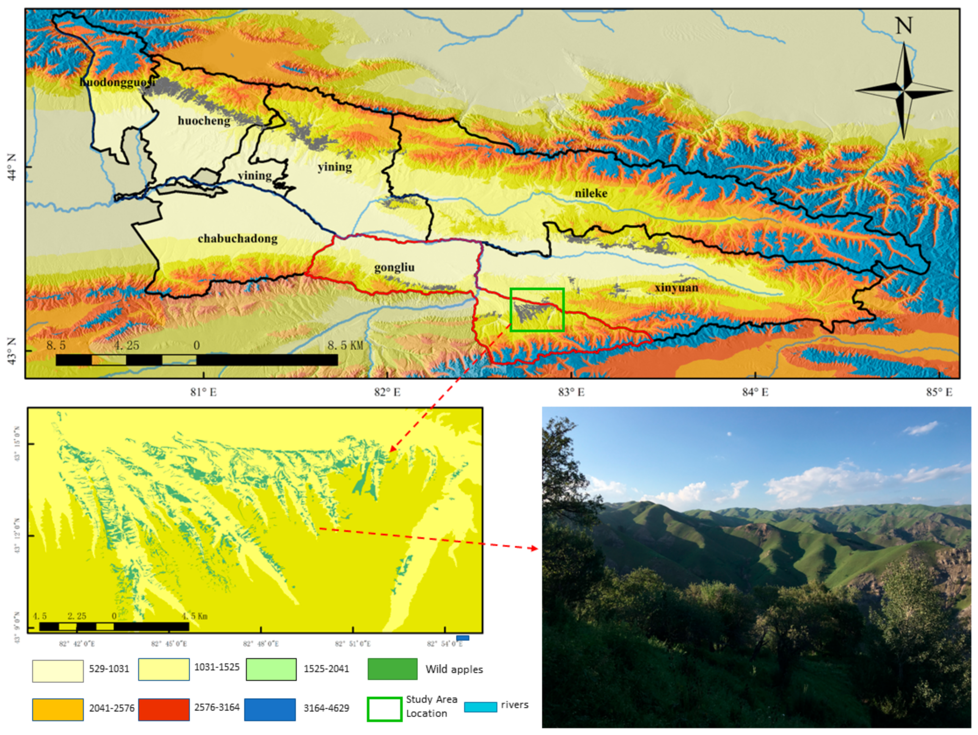
Based on landscape and ecological theories, this study uses four periods of remote sensing images of 1964, 1980, 2000, and 2017 as data sources, focuses on the MF area in the Mohe watershed of the Ili River valley in Xinjiang, applies the InVEST model to assess the spatial and temporal changes in habitat quality under four periods of landscape pattern distribution, and investigates the relationship between landscape pattern changes and habitat quality. Then, we use principal component analysis to identify the driving forces of landscape pattern changes. The objectives of this study are the following: (1) obtain appropriate parameters for the MF‘s susceptibility to threat factors; (2) assess the spatiotemporal variation in habitat quality in the period of 1964–2017; (3) identify the characteristics of spatial differentiation of habitat quality from ecosystem perspectives; and (4) analyze the underlying correlations between the influencing factors and habitat quality. The study may help us comprehend how the dynamics of landscape patterns affect biodiversity and help local governments make decisions for the preservation of biodiversity and landscape planning in MF area.

2. Materials and Methods

2.1. Study Area

The study area is situated in the eastern portion of Gongliu County, Ili Kazakh Autonomous Prefecture, Xinjiang Uygur Autonomous Region, on the western part of the Central Tianshan Mountains, on the south bank of the Jirgulang River, and in the Mohe watershed on the northern slope of the Narathi Mountains. The geographical coordinates were 43°10′–43° 14′ N with a longitude of 82°43’–82°52′ E, an elevation of 1100–1600 m, and a ground relative elevation difference of 200–350 m [22]. This area has the continental climate of the north temperate zone, with an average annual temperature of 4 °C, a frost-free period of 105 d, precipitation of 550 mm, and a snow cover period of 95 d. Wild apple, wild apricot (Armeniaca vulgaris), wild hawthorn (Crataegus chlorocarpa), rowan (Sorbus tianschanica), thick plum (Padus racemosa), and other trees are the predominant trees in this region. The main herbs include fescue (Festuca gigantea), motherwort, and rose (Rosa acicularis), while the main shrubs are berberis [23] (Figure 1 depicts the zone’s location).

2.2. Data Sources and Preprocessing

In this study, photos from the MF area taken by CORONA/SPOT/GF-2 satellites in 1964, 1980, 2000, and 2017 were utilized as data sources (

Table 1. Data Resources.

Data Resources	Scene ID	Date	Resolution
CORONA Satellite	DS09058A054MC037	29 August 1964	2.5 m
CORONA Satellite	DZB1216-500108L005001	10 July 1980	10 m
SPOT Satellite	42082630011030546462M	3 November 2000	2.5 m
GF-2	4221681	17 October 2017	1 m

). Images with low cloudiness, all within 10 m resolution, were chosen. The four preprocessing steps of remote sensing images—image radiation correction, picture fusion, waveband selection, image stitching, and cropping—were performed using ENVI5.3. A mix of supervised classification and visual interpretation was utilized, and Google Earth maps, a forest resource survey, and in situ survey data were used to verify the correctness of the interpretation findings. Referring to the classification criteria of the 2017 national land use status classification system (GB/T21010-2017) and the land classification system of the Chinese Academy of Sciences [24,25], the landscape pattern of the MF area was classified according to the characteristics of the study area [22]. The final distribution of landscape types in the Mohe watershed of the MF area was obtained. It was concluded from the test that the kappa coefficients of all four periods were more significant than 80%, and the accuracy of landscape classification met the research requirement criteria.

2.3. Landscape Classification and Accuracy Verification

This research employs the maximum likelihood method [26] to categorize the photos using a combination of supervised classification and manual interpretation by the landscape classification system. When remote sensing photos are expressly utilized for post analysis, the accuracy of the categorized images must also be evaluated because there invariably are errors and omissions. The Kappa coefficient can more accurately indicate classification accuracy [27,28]. The 1964 Malus sieversii resource results were verified using the 1964 remote sensing images, and some visual interpretation was added to and improved upon using the first forest resource class II survey data of the study area (based on the 1:50,000 aerial photo interpretation and interview survey in the late 1950s). The second forest resource class II survey data of the study area (based on the 1:25,000 aerial photo interpretation in 1980) were used to verify the 1964 MF resource results, and these results were then used to determine the extent to which the MF resource overall classification accuracy was 93.6542%; the Kappa coefficient was 0.8463, and the classification accuracy was 91.2569% overall. Based on the 1964 remote sensing images, the first forest resource class II survey data of the study area (based on the 1:50,000 aerial photo interpretation and interview survey in the late 1950s) were used to verify the 1964 MF resource with some visual interpretation to supplement and improve it; the second forest resource class II survey data of the study area (based on the 1:25,000 aerial photo interpretation in 1980) were used as well. Respectively, the overall classification accuracy was 91.2569%, and the Kappa coefficient was 0.8123; the overall classification accuracy was 93.6542%, and the Kappa coefficient was 0.8463. The overall classification accuracy was 94.2569%, and the kappa coefficient was 0.8642. The accuracy of the landscape classification results met the research requirements.

2.4. Landscape Metrics

The landscape type transfer matrix for 1964–1980, 1980–2000, 2000–2017, and 1964–2017, respectively, were obtained by superimposing and analyzing the landscape type maps from 1964, 1980, 2000, and 2017, and the transfer area matrix recorded the area of each landscape type converted to other landscape types.

Different landscape indices were chosen to further investigate the landscape pattern evolution characteristics of the MF region, and the Patch Analysis module of Fragstats 4.0 was utilized to calculate the landscape pattern metrics. Through comparative analysis, the following indices were selected: number of patches (NP), patch density (PD), contagion index (CONTAG), Shannon’s diversity index (SHDI), Shannon’s evenness index (SHEI), and cohesion index (COHESION) to quantitatively characterize the landscape pattern changes (

Table 2. Landscape pattern index.

Landscape Metrics	Mathematical Expression	Subscripts/Symbols
Number of patches (NP)	$NP=n_i$	$n_i$ = total number of patches in the landscape. $a_{\mathit{ij}}$ = area (m2) of patch $\mathit{ij}$ $g_{\mathit{ik}}$ = number of adjacencies (joins) between pixels of patch types (classes) $i$ and $k$ based on the double-count method. $p_i$ = proportion of the landscape occupied by patch type (class) $i$. $p_{\mathit{ij}}$ = perimeter of patch $\mathit{ij}$ in terms of number of cell surfaces.
Patch density (PD)	$\mathit{PD}=\frac{n_i}{a_{\mathit{ij}}}\times 100$
Contagion index (CONTAG)	$\mathit{CONTAG}=1+\frac{{\displaystyle \sum _{i=1}^m{\displaystyle \sum _{k=1}^m\left[\left(P_i\right)\left(\frac{g_{\mathit{ik}}}{{\displaystyle \sum _{k=1}^m{g}_{\mathit{ik}}}}\right)\right]}}\cdot \left[\ln {(P)}_i\left(\frac{g_{\mathit{ik}}}{{\displaystyle \sum _{k=1}^m{g}_{\mathit{ik}}}}\right)\right]}{2{\log }_e(m)}\times 100$
Shannon’s diversity index (SHDI)	$\mathit{SDHI}=-{\displaystyle \sum _{i=1}^m\left(P_i{\log }_e{P}_i\right)}$
Shannon’s evenness index (SHEI)	$\mathit{SHEI}=\frac{-{\displaystyle \sum _{i=1}^m\left(P_i{\log }_e{P}_i\right)}}{{\log }_{e}m}$
Cohesion index (COHESION)	$\mathit{COHESION}=\left[1-\frac{{\displaystyle \sum _{i=1}^m{\displaystyle \sum _{j=1}^n{p}_{\mathit{ij}}}}}{{\displaystyle \sum _{i=1}^m{\displaystyle \sum _{j=1}^n{p}_{\mathit{ij}\sqrt{a_{\mathit{ij}}}}}}}\right]{\left[1-\frac{1}{\sqrt{A}}\right]}^{-1}\times 100$

) [29].

2.5. Habitat Quality Calculation Based on InVEST Model

The habitat quality module of the InVEST model was chosen for this study to evaluate the characteristics of habitat change at the landscape level in the MF area. The following threat factors were used: cultivated land, landslide areas, roads, and residential building sites. The maximum impact distance, weights, habitat types, and sensitivity of threat factors were assigned by the manual of the InVEST model and examples of the InVEST model, combined with related studies [23,24,25,26,27,28,29,30,31,32,33,34,35,36], as shown in

Table 3. The maximum influence distance and weight of different threat factors.

Threat Factors	Maximum Influence Distance	Weights	Habitat Type
Cultivated land	1.0	0.6	Linear
Landslide	0.5	1.0	Exponential
Roads	0.5	0.4	Linear
Buildings	2.0	0.5	Linear

and

Table 4. Habitat adaptability of different landscapes and their sensitivity to various threat factors.

Landscape Type	Habitat Adaptability	Cultivated Land	Landslide	Roads	Buildings
Wild apples	1.0	0.5	0.8	0.3	0.4
Other forest land	0.8	0.5	0.7	0.4	0.4
Grassland	0.9	0.8	0.8	0.2	0.3
Cultivated land	0.0	0.0	0.2	0.0	0.0
Water	1.0	0.3	0.0	0.0	0.2
Landslide	0.0	0.1	0.0	0.2	0.3
Roads	0.0	0.0	0.3	0.0	0.0
Buildings	0.0	0.0	0.1	0.0	0.0

.

Habitat degradation degree represents how environmental risk factors impact specific landscape-type raster cells. The higher the score, the more the raster cell is affected by threat factors; a higher habitat quality score reflects good or poor habitat quality under the influence of threat sources; the higher the score, the more stable the ecosystem, and the higher the habitat quality; and the lower the score, the more vulnerable the ecological environment is to external disturbance.

Table 5. Habitat evaluation indices and meaning.

Habitat Evaluation Indicators	Mathematical Expression	Meaning
Degree of habitat degradation	(1) ${\mathrm{D}}_{\mathit{xj}}={\displaystyle \sum _{r=1}^R{\displaystyle \sum _{y=1}^{r_r}\left(\frac{W_r}{{\displaystyle \sum _{r=1}^R{\omega }_r}}\right)}}{r}_y{i}_{\mathit{nxy}}{\beta }_x{S}_{\mathit{jr}}$	Dxj: habitat degradation degree of raster x, indicating the degree of habitat degradation exhibited by pressure; R: number of threat factors; wr: threat factor weights; Yr: number of rasters of the threat layer on the ground class layer; ry: intensity of threat factors, number of threat factors on each raster; irxy: threat level of the threat factor to the habitat; βx: degree of legal protection; Sjr: denotes the level of sensitivity of land type j to threat factors; dxy: distance between raster x (habitat) and raster y (threat factor); drmax: the maximum impact range of the threat factor r
	(2) $i_{\mathit{rxy}}=1-\left(\frac{d_{\mathit{xy}}}{d_{r\max }}\right)$
Habitat quality	(3) $Q_{\mathit{xj}}=H_j\left[1-\left(\frac{D_{\mathit{xj}}^z}{D_{\mathit{xj}}^z+k^z}\right)\right]$	Qxj: habitat quality index of the j landscape type x raster; Hj: habitat suitability score for the j landscape type, with values ranging from 0 to 1; z: 2.5; k: half-saturation constant, i.e., half of the maximum value of habitat degradation

displays the indices for evaluating habitat quality and their respective definitions.

2.6. Driving Factors of Landscape Pattern Change

The change in landscape pattern results from the interaction between natural and human factors. This paper combines the actual situation of the MF area in the Mohe watershed and divides the indicators into 4 major categories (environmental, economic, demographic, and social) and 12 indicators (X1 to X12) based on qualitative and quantitative research. (

Table 6. Malus sieversii forest‘s Driving Force Index System in the Mohe Basin.

Target Layer	Element Layer	Indicator Layer
Natural factors	Environmental factors	Average temperature (X1), annual precipitation (X2), area of collapse (X3)
Human factors	Economic factors	Grain production (X4), oil production (X5), farmers’ and herders’ income (X6)
	Demographic factors	Population (X7), agricultural population (X8)
	Social factor	Woodcutting (X9), cultivation (X10), total livestock stock (X11), pastoral output (X12)

and

Table 7. Driver eigenvalues and main contribution rate.

Indicator Factors	Eigenvalue	Contribution Rate %	Cumulative Contribution Rate %
X1	10.723	89.356	89.356
X2	0.942	7.846	97.202
X3	0.336	2.798	100
X4	3.34752 × 10−16	2.7896 × 10−15	100
X5	2.3648 × 10−16	1.97067 × 10−15	100
X6	1.74958 × 10−16	1.45798 × 10−15	100
X7	8.87243 × 10−17	7.39369 × 10−16	100
X8	7.12545 × 10−17	5.93788 × 10−16	100
X9	1.24238 × 10−16	1.03531 × 10−15	100
X10	1.96251 × 10−16	1.63543 × 10−15	100
X11	3.28664 × 10−16	2.73887 × 10−15	100
X12	5.53737 × 10−16	4.61448 × 10−16	100

).

Principal component analysis was performed on the driving factors, and the obtained driver eigenvalues and principal contributions (Table 7) and principal component rotated loading matrix (

Table 8. Main component rotation load matrix.

Indicator Factors	F1	F2	F3
X1	0.958	0.191	−0.216
X2	0.865	0.501	0.034
X3	0.838	−0.525	0.151
X4	0.978	0.111	0.176
X5	0.903	0.002	−0.029
X6	0.970	0.114	0.216
X7	0.987	−0.005	−0.160
X8	0.962	0.111	−0.249
X9	0.952	0.261	0.211
X10	0.863	−0.505	−0.002
X11	0.993	0.079	0.083
X12	0.970	0.108	0.220

) indicate that the cumulative contribution of the first three principal components reached 100%, which means that the first three principal components represent all the information in the 12 indicators.

3. Results

3.1. Landscape Pattern Change Analysis

Since the area of road and river landscapes changed between 1964 and 2017, they were omitted from the transfer matrix for the time being. More than 90 percent of the research area is comprised of the MF, grasslands, and other woodlands (coniferous forests, broad-leaved forests, and mixed coniferous forests).

Table 9. Area transfer matrix of landscape types from 1964 to 2017 in Mohe Watershed (hm²).

Era	Land Type	Wild Apple	Other Forest Land	Grassland	Cultivated Land	Landslide	Buildings
1964–1980	Wild apple	-	4.87	1850.32	11.92	0.00	0.06
	Other forest land	141.56	-	7.99	0.00	0.00	0.00
	Grassland	21.20	15.14	-	317.00	0.00	77.77
	Cultivated land	1.04	0.00	20.38	-	0.00	0.00
	Landslide	0.00	0.00	0.00	0.00	-	0.00
	Buildings	7.41	0.02	13.06	2.95	0.00	-
1980–2000	Wild apple	-	111.38	2001.53	163.09	80.60	31.63
	Other forest land	14.97	-	1111.84	227.29	41.25	8.52
	Grassland	364.54	593.96	-	930.47	114.53	173.97
	Cultivated land	0.80	12.04	16.37	-	0.00	61.42
	Landslide	9.89	4.27	11.76	0.00	-	0.00
	Wild apple	0.00	0.00	0.67	20.66	0.00	-
2000–2017	Other forest land	-	0.07	86.24	4.68	4.89	0.00
	Grassland	16.77	-	24.44	0.00	1.83	0.00
	Cultivated land	15.35	1.20	-	8.69	15.32	0.58
	Landslide	0.48	0.05	40.25	-	0.11	43.09
	Buildings	2.27	5.05	21.82	0.00	-	0.00
	Wild apple	0.00	0.00	9.79	24.81	0.00	-
1964–2017	Wild apple	-	148.80	3620.51	267.52	93.32	2.22
	Other forest land	125.67	-	1119.41	236.70	38.70	15.82
	Grassland	246.07	525.85	-	1018.19	96.70	325.17
	Cultivated land	0.81	12.04	12.97	-	0.00	0.01
	Landslide	9.65	4.27	11.30	0.00	-	0.00
	Building site	0.00	0.02	6.27	18.92	0.00	-

demonstrates that the landscape pattern of the study area has changed between 1964 and 2017. The changes in various types of landscapes are primarily manifested by the annual decrease in the area of the MF and other woodlands (coniferous forests, broad-leaved forests, and mixed coniferous forests) and the annual increase in the area of cultivated land, residential construction land, and landslides. Among them, the area of the MF declined from 6239.7 hm² to 2440.89 hm². The main inflow landscapes are grassland and other forest lands, 246.07 hm² and 125.67 hm², respectively, while the main outflow landscapes are grassland and cultivated land, 3620.51 hm² and 267.52 hm², respectively. The area of the MF is diminished owing to overexploitation by humans, and the MF is also impacted by the apple small giddy insect pest, which causes forest trees to die. The cultivated land area expanded from 1425.6 hm² to 2944.26 hm²; the major transfer in the landscape is grassland, MF, and other woodlands, which are 1018.19 hm², 267.52 hm², and 236.7 hm², respectively; and the main transfer-out landscape is grassland and other woodlands, 12.97 hm² and 12.04 hm², respectively. The inflow area is bigger than the outflow area, and it can be observed that the amount of cultivated land expands and large areas of reduced grassland and MF are reclaimed as farmland. The main increase in the grassland landscape is in the MF and other woodlands, 3620.51 hm² and 1119.41 hm², respectively, and the outflow is cultivated land and other woodlands, 1018.19 hm² and 525.85 hm², respectively, indicating that humans destroy grassland on a large scale for production and living and destroy woodland through disturbance in addition to degrading woodland landscapes into grassland landscapes and destroying the stability of the ecosystem.

From the landscape level index analysis, NP and PD indices in the study area increased from 2548 and 9.9956 to 5397 and 21.1719, respectively, from 1964 to 2017, and AREA_MN decreased from 10.0045 to 4.7233. The CONTAG index increased from 64.6579. AREA_MN decreased from 10.0045 to 4.7233. The CONTAG index decreased from 64.6579 to 63.9887, indicating that the fragmentation of the entire MF area increased as a result of human disturbance, malachite small giddy insect pests, and geological disasters, posing a particular threat to the ecological balance and habitat quality of the area. The SHEI and SHDI declined from 0.6425 and 1.4116 to 0.6373 and 1.4002, respectively, showing a declining trend in landscape diversity and an unavoidable deterioration of the landscape’s structural equilibrium.

3.2. Analysis of Spatial and Temporal Variation in Habitat Quality

The habitat quality was divided into six classes according to the habitat quality score, which was 0–0.1, 0.1–0.2, 0.2–0.4, 0.4–0.6, 0.6–0.8, and 0.8–1.0, and the spatial and temporal characteristics of habitat quality were analyzed as shown in

Table 10. Spatial statistics of habitat quality of wild apple forest in the Mohe Basin from 1964 to 2017.

Habitat Quality Score	1964			1980			2000			2017
	Area Weight /%	Mean Habitat Quality	Standard Deviation	Area Weight /%	Mean Habitat Quality	Standard Deviation	Area Weight /%	Mean Habitat Quality	Standard Deviation	Area Weight /%	Mean Habitat Quality	Standard Deviation
0–0.1	6.3			10.73			17.92			18.76
0.1–0.2	10.68			14.23			20.46			17.95
0.2–0.4	12.19	0.7153	0.3721	10.2	0.6691	0.376	5.37	0.637	0.4031	5.69	0.6411	0.4024
0.4–0.6	0.57			1.71			2.95			3.83
0.6–0.8	1.98			2.42			3.48			3.62
0.8–1.0	68.28			60.71			49.82			50.15

. In terms of time series, the mean habitat quality in the Mohe watershed MF region was 0.7153 in 1964, 0.6691 in 1980, 0.637 in 2000, and 0.6411 in 2017, with a general downward trend. The rise in the standard deviation of habitat quality from 0.3721 to 0.4024 indicates that the variation in habitat quality among raster cells increased, suggesting a general trend of habitat quality decline.

Figure 2 displays the regional and temporal trend of habitat quality in the Mohe watershed’s MF zone from 1964 to 2017. As seen in the figure, the area between 0 and 0.1 of the habitat quality score of the MF area is expanding, primarily in the north and northeast of the study area, where the habitat quality is relatively poor due to the area being a plain, cultivated land and residential construction land are primarily used, and human activities are frequent, superimposed on the apple girdling insect pest; the densely distributed area of the MF in the center of the study area is decreasing in size. Due to the frequent occurrence of geological hazards, such as landslides and the effect of insect pests, the habitat quality is reduced in the central area of the research zone, resulting in a significant loss of the MF. The ecology is more stable in the south’s high-altitude regions, less impacted by nature and people.

3.3. Correlation Analysis of Malus sieversii Forest Habitat Quality and Landscape Pattern

Based on temporal and spatial distribution of landscape types of MF areas in the Mohe watershed (Figure 3) and Spatial and temporal distribution characteristics of habitat quality. (Figure 4), we found that the habitat quality in the northern part of the study area is more variable because the northern part is dominated by cultivated land patches and residential building land patches, and the larger the maximum patch area, the worse the habitat quality under stress in the area. The dominant distribution landscape in the central region is MF, and in areas dominated by MF, the larger the size of MF patches, the greater the ecological service value. In contrast, reducing the amount of MF patches harms ecosystem function and habitat quality. Consequently, there is a link between habitat quality and landscape pattern, and the influence of the same landscape index on the habitat quality of distinct landscape types in different locations varies [37].

According to Figure 3, from 1964 to 2017 in the MF area of the Mohe watershed, the landscape area of MF and other woodlands (coniferous, broad-leaved, and quasi-broad mixed forests) decreased by 60.88% and 16.50%, respectively, the area of cultivated land increased by 51.58%, the area of landslides increased by 68.18%, and the floor area increased by 85.06%. When comparing Table 10 and Figure 4, it can be observed that the amount of land with a habitat quality score of 0.8–1.0 fell by 18.13% between 1964 and 2017, but the area of land with a habitat quality score of 0–0.1 or 0.1–0.2 rose by 12.46% and 7.27%, respectively. Thus, human activity disruption and natural catastrophes such as landslides are the primary causes of the change in landscape patterns and the primary drivers of changes in habitat quality. Therefore, the influence of human and natural factors should be fully considered in habitat protection and ecological planning and control of the MF area in the south Tianshan mountain.

4. Discussion

Influence of Various Factors on the Landscape of Malus sieversii Forests

Landscape pattern changes result from a combination of multiple factors [38]. The population factor is one of the indirect causal factors of dynamic changes in the Mohe watershed MF area. Its influence may indirectly induce changes in the MF landscape by acting on other factors. In addition, the influence of many uncertain factors, such as natural pests and diseases, fires, and landslides, lead to more complex changes in the MF area in the Mohe watershed, as well as changes that are difficult to determine. From a short period, the frequency and rate of changes in natural factors are slower than those of human factors, and their influence on landscape pattern changes is not apparent. However, from a more extended period, their influence on landscape pattern changes is significant. Data show that the study area’s population in 2017 was 4.2 times that of 1964, and the population has increased relatively rapidly in recent decades. The increase in population has not only increased the labor force but also brought about many resource supply carrying capacity problems so that the per capita area of cultivated land, grassland, and forest land has decreased, and to meet the needs of production and living, the acquisition of natural resources must be increased, and the demand for reclaimed cultivated land has been increasing. The reason is that, to protect the ecological environment, the Chinese government actively advocates the implementation of the policy of returning farmland to forest land and grassland so that farmland is transformed into grassland and woodland. From the analysis of the MF landscape area, we find that it is also consistent with this change. The analysis of the area found that it also conforms to this changing pattern, and the area decreased more before 2000. After 2000, the change tends to level off, demonstrating that the change in cultivated land area is one of the key factors influencing the transformation of the MF‘s landscape pattern. From 1964 to 2017, the income of farmers and herders in the study area showed an upward trend, demonstrating how economic growth can support society’s ongoing advancement and development. However, for economic growth at the same time, farmers and herders inevitably reclaim grassland and forest land into cultivated land and cut trees for fuel. However, before 2000, economic growth was slow due to the lack of high technology and limited food production. After 2000, economic growth was accelerated with the improvement of technology, intensive production, and the transformation of multiple business methods. The increase in the income of farmers and herders has changed the distribution of the landscape pattern of Malus sieversii.

Moreover, temperature changes significantly impact the distribution of landscape patterns [39]. In the context of global warming, the study area has experienced a significant increase in temperature and precipitation from 1960 to the present [40], which has caused the MF landscape to shift toward higher elevations, as evidenced by the large areas of 0-10-year-old Sevier apple seedlings and multiple 20–30-year-old Sevier apple forests growing above the birch tree line in the field survey, which exceeded the upper elevation of the 1600m MF. This is reinforced by the enormous regions of 0–10-year-old sieversii apple seedlings and 20–30-year-old sieversii apple stands growing above the birch forest line on the mountain peaks. The influence of temperature and human activities to the extent that the landscape area of MF in lower elevation areas is decreasing and being replaced by other landscape types has led to an increase in landscape instability and a high likelihood of shifting to grassland landscapes, as well as a decrease in coverage and area and a gradual increase in fragmentation. Moreover, the distribution pattern has become more complex.

The influence of precipitation and collapse on the landscape of MF results from various factors acting together. The study area is located at the mouth of the river, a layer of loess of several meters covers the bedrock of the surface to tens of meters of thickness, the loess is soft and poorly compacted, and overload grazing is expected in the area, which often leads to surface exposure. This is also why this element has become the dominant factor in the landscape change of MF.

In addition, the influence of many uncertain factors, such as natural pests and diseases, fires, landslides, and landslide hazards, leads to more complex changes in the MF area in the Mohe watershed as well as changes that are difficult to determine. In a short period, the frequency and rate of change in natural factors are slower than those in human factors, and the impact on changes in landscape patterns is not apparent. However, in a more extended period, the impact of changes in landscape patterns is significant.

5. Conclusions

Using the Mohe watersheds as an example, this study integrated the InVEST-based model to examine the spatial and temporal changes in landscape patterns and habitat quality in the MF area from 1964 to 2017. The results of the study are as follows.

(1)

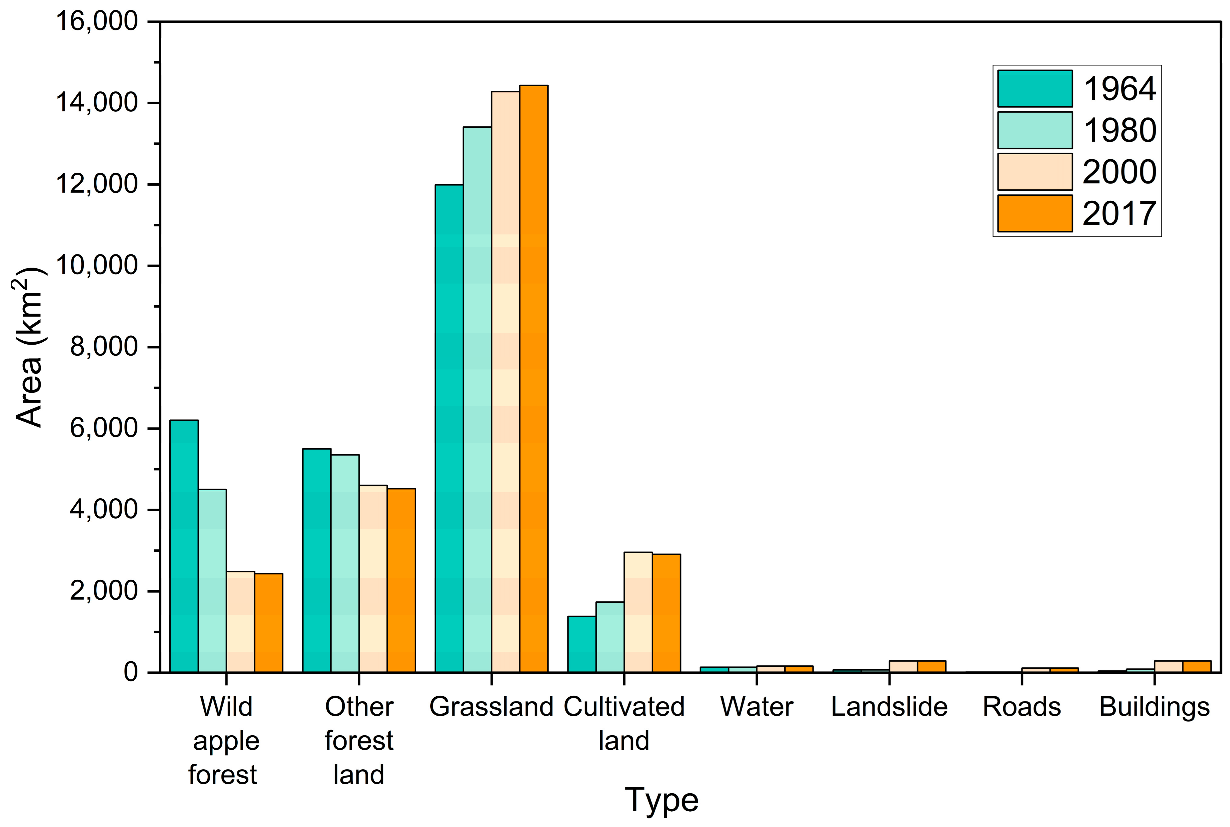
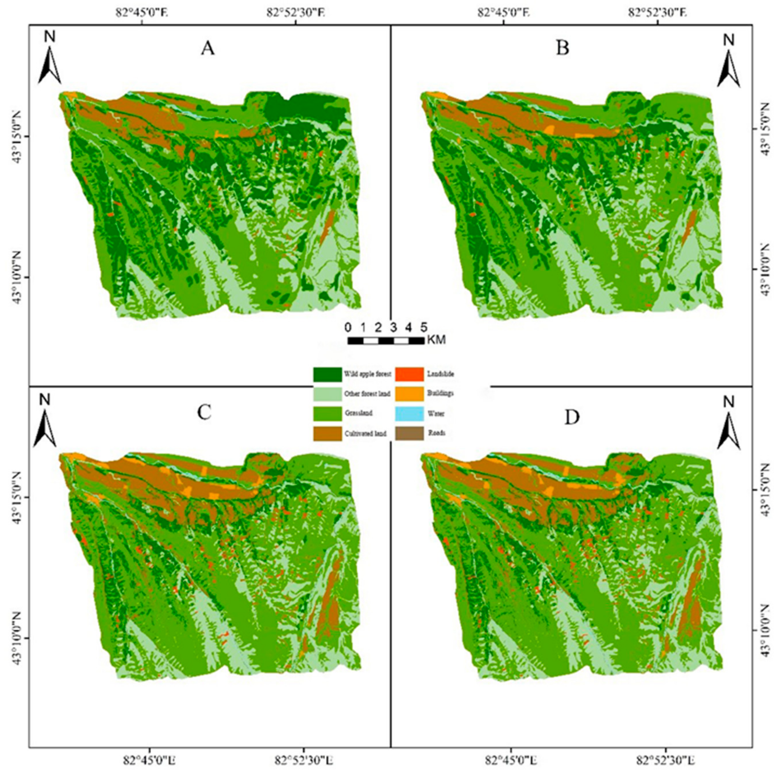
The landscape layout of the MF region in the Mohe watersheds has changed between 1964 and 2017. The number of Malus sieversii and other woodlands (coniferous, broad-leaved, and mixed coniferous forests) dropped annually. At the same time, grassland and cultivated land were the most productive landscapes. Annual increases in buildings, cultivated land, and landslides indicate that the area of the MF is under the influence of human interference and climate change at this time. Each landscape measure reveals that the fragmentation of the entire study area has increased and the stability of the ecosystem has decreased, posing a threat to the ecological balance and habitat quality in the region.

(2)

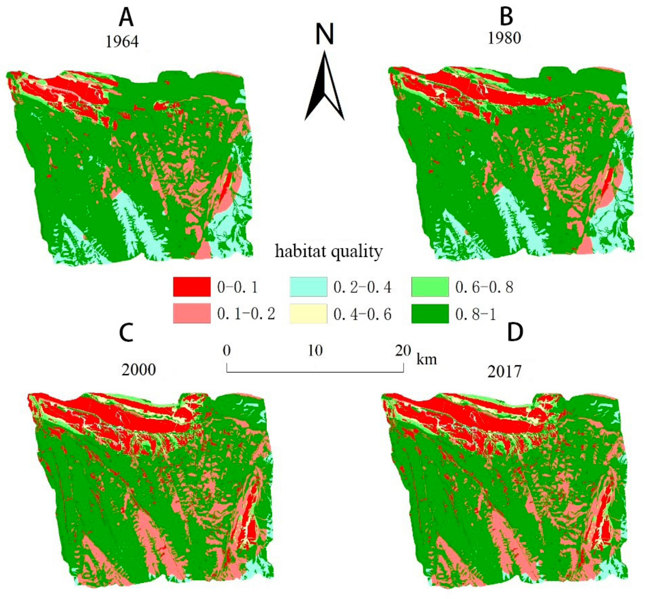
From 1964 to 2017, a regional and temporal analysis of the habitat quality of the entire research area revealed a downward trend. Low habitat values are primarily distributed in the north and northeast because this is a plain area where cultivated land and buildings are prevalent and human activities are frequent; the central part of the study area shows scattered habitat low-value areas, which mainly exist in landslides, mudslides, and other geological disaster-prone areas; and the high-altitude area in the south is less disturbed by natural and human interference and has a higher habitat value.

(3)

The habitat quality in the northern section of the research area is more variable, and because the northern region is dominated by cultivated land patches and building patches, the greater the maximum patch area, the less the habitat quality is impacted in this region. In the central region, the dominant distribution landscape is MF, and in the area dominated by MF, the greater the area of MF patches, the greater the value of ecological services, whereas a reduction in its area leads to a decline in ecosystem function, which in turn affects the habitat quality grade. Therefore, there is a correlation between habitat quality and landscape pattern, and there is variation in the influence of the same landscape index on the habitat quality of distinct landscape types in various regions [41].

In summary, this study showed that, from 1964 to 2017, the whole study area’s habitat quality showed a deteriorating tendency after a regional and temporal analysis and that several factors including climate change and human activity have caused the habitat to weaken. Additionally, there lies a correlation between landscape pattern and habitat quality. However, all factors on MF in the InVEST model are simply summed, while the total impact of multiple threats is always much larger than the arithmetic sum of various impacts. Therefore, how to scientifically integrate multiple ecosystem services in watersheds in the future and analyze in depth the complex relationships between different ecosystem services is important. Finally, the results of this study can provide scientific support for managing and protecting MF in China.

References

1. Chen, X.; Feng, T.; Zhang, Y.; He, T.; Feng, J.; Zhang, C. Genetic diversity of volatile components in Xinjiang Wild Apple (Malus sieversii). J. Genet. Genom. 2007, 34, 171–179. [Google Scholar] [CrossRef]
2. Chen, L. The Current Situation of Biodiversity in China and Its Protection Countermeasures; Science Press: Beijing, China, 1993; pp. 194–197. [Google Scholar]
3. Wang, N.; Jiang, S.; Zhang, Z.; Fang, H.; Xu, H.; Wang, Y.; Chen, X. Malus sieversii: The origin, flavonoid synthesis mechanism, and breeding of red-skinned and red-fleshed apples. Hortic. Res. 2018, 5, 70. [Google Scholar] [CrossRef] [PubMed] [Green Version]
4. Qian, Y.K.; Ma, K.P. Principles and Methods of Biodiversity Research; China Science and Technology Press: Beijing, China, 1994; pp. 141–157. [Google Scholar]
5. Yang, Y. Evolution of habitat quality and association with land-use changes in mountainous areas: A case study of the Taihang Mountains in Hebei Province, China. Ecol. Indic. 2021, 129, 107967. [Google Scholar] [CrossRef]
6. Goldstein, J.H.; Caldarone, G.; Duarte, T.K.; Ennaanay, D.; Hannahs, N.; Mendoza, G.; Polasky, S.; Wolny, S.; Daily, G.C. Integrating ecosystem-service tradeoffs into land-use decisions. Proc. Natl. Acad. Sci. USA 2012, 109, 7565–7570. [Google Scholar] [CrossRef] [Green Version]
7. Nelson, E.; Mendoza, G.; Regetz, J.; Pola, S.; Tallis, H.; Cameron, D. Modeling multiple ecosystem services, biodiversity conservation, commodity production, and tradeoffs at landscape scales. Front. Ecol. Environ. 2009, 7, 4–11. [Google Scholar] [CrossRef]
8. Liu, S.; Liao, Q.; Xiao, M.; Zhao, D.; Huang, C. Spatial and Temporal Variations of Habitat Quality and Its Response of Landscape Dynamic in the Three Gorges Reservoir Area, China. Int. J. Environ. Res. Public Health 2022, 19, 3594. [Google Scholar] [CrossRef]
9. Zhang, X.; Zhou, J.; Li, G.; Chen, C.; Li, M.; Luo, J. Spatial pattern reconstruction of regional habitat quality based on the simulation of land use changes from 1975 to 2010. J. Geogr. Sci. 2020, 30, 601–620. [Google Scholar] [CrossRef]
10. Gustafson, E.J. Quantifying landscape spatial pattern: What is the state of the art? Ecosystems 1998, 1, 143–156. [Google Scholar] [CrossRef]
11. Zhu, C.; Zhang, X.; Zhou, M.; He, S.; Gan, M.; Yang, L.; Wang, K. Impacts of urbanization and landscape pattern on habitat quality using OLS and GWR models in Hangzhou, China. Ecol. Indic. 2020, 117, 106654. [Google Scholar] [CrossRef]
12. Chu, L.; Sun, T.; Wang, T.; Li, Z.; Cai, C. Evolution and prediction of landscape pattern and habitat quality based on CA-Markov and InVEST model in Hubei section of Three Gorges Reservoir Area (TGRA). Sustainability 2018, 10, 3854. [Google Scholar] [CrossRef]
13. Gong, J.; Xie, Y.; Cao, E.; Huang, Q.; Li, H. Integration of InVEST-habitat quality model with landscape pattern indexes to assess mountain plant biodiversity change: A case study of Bailongjiang watershed in Gansu Province. J. Geogr. Sci. 2019, 29, 1193–1210. [Google Scholar] [CrossRef] [Green Version]
14. Xu, L.; Chen, S.S.; Xu, Y.; Li, G.; Su, W. Impacts of land-use change on habitat quality during 1985–2015 in the Taihu Lake Basin. Sustainability 2019, 11, 3513. [Google Scholar] [CrossRef] [Green Version]
15. Sherrouse, B.C.; Clement, J.M.; Semmens, D.J. A GIS application for assessing, mapping, and quantifying the social values of ecosystem services. Appl. Geogr. 2011, 31, 748–760. [Google Scholar] [CrossRef]
16. Wu, X.; Hu, F. Analysis of ecological carrying capacity using a fuzzy comprehensive evaluation method. Ecol. Indic. 2020, 113, 106243. [Google Scholar] [CrossRef]
17. Li, J.; Zhang, X. Evaluation of ecological environment quality in resource-based cities—A case study of Hegang city. Resour. Ind. 2011, 13, 6–10. [Google Scholar]
18. Tallis, H.; Ricketts, T.; Guerry, A.; Wood, S.A.; Chaplin-Kramer, R. InVEST User’s Guide: Integrated Valuation of Environmental Services and Tradeoffs; The Natural Capital Project: Stanford, CA, USA, 2013. [Google Scholar]
19. Terrado, M.; Sabater, S.; Chaplin-Kramer, B.; Mandle, L.; Ziv, G.; Acuña, V. Model development for the assessment of terrestrial and aquatic habitat quality in conservation planning. Sci. Total Environ. 2016, 540, 63–70. [Google Scholar] [CrossRef] [PubMed] [Green Version]
20. Lin, Y.P.; Lin, W.C.; Wang, Y.C.; Lien, W.Y.; Huang, T.; Hsu, C.C.; Schmeller, D.S.; Crossman, N.D. Systematically designating conservation areas for protecting habitat quality and multiple ecosystem services. Environ. Model. Softw. 2017, 90, 126–146. [Google Scholar] [CrossRef]
21. Zhang, Y.; Zhang, C.; Zhang, X.; Wang, X.; Liu, T.; Li, Z.; Lin, Q.; Jing, Z.; Wang, X.; Huang, Q.; et al. Habitat Quality Assessment and Ecological Risks Prediction: An Analysis in the Beijing-Hangzhou Grand Canal (Suzhou Section). Water 2022, 14, 2602. [Google Scholar] [CrossRef]
22. Li, L.; Chen, S.J.; Chen, M.Y.; Zhang, X.; Jia, X. Environmental driving force of stool shoot quantitative features of Malus sieversii (Ldb.) in Xiaomohe valley. Ecol. Sci. 2019, 38, 18–24. [Google Scholar]
23. Wang, Q.; Li, W.; Wu, Y.; Pei, Y.; Xie, P. Application of statistical index and index of entropy methods to landslide susceptibility assessment in Gongliu (Xinjiang, China). Environ. Earth Sci. 2016, 75, 599. [Google Scholar] [CrossRef]
24. Liu, J. Macro Investigation and Dynamic Analysis of Remote Sensing of Resources and Environment in China; China Science and Technology Press: Beijing, China, 1996; pp. 23–28. [Google Scholar]
25. Zhang, H.; Xu, E.; Zhu, H. Ecological-Living-Productive Land Classification System in China. J. Resour. Ecol. 2017, 8, 121–128. [Google Scholar]
26. Bolstad, P.; Lillesand, T.M. Rapid maximum likelihood classification. Photogramm. Eng. Remote Sens. 1991, 57, 67–74. [Google Scholar]
27. Ma, Z.; Redmond, R.L. Tau coefficients for accuracy assessment of classification of remote sensing data. Photogramm. Eng. Remote Sens. 1995, 61, 435–439. [Google Scholar]
28. Ben-David, A. Comparison of classification accuracy using Cohen’s Weighted Kappa. Expert Syst. Appl. 2008, 34, 825–832. [Google Scholar] [CrossRef]
29. Peng, J.; Wang, Y.; Zhang, Y. Influence of land use classification on landscape pattern index. Acta Geogr. Sin. 2006, 61, 157–168. [Google Scholar]
30. Morris, E.K.; Caruso, T.; Buscot, F.; Fischer, M.; Hancock, C.; Maier, T.S.; Meiners, T.; Müller, C.; Obermaier, E.; Prati, D.; et al. Choosing and using diversity indices: Insights for ecological applications from the German Biodiversity Exploratories. Ecol. Evol. 2014, 4, 3514–3524. [Google Scholar] [CrossRef]
31. Wang, X.; Blanchet, F.G.; Koper, N. Measuring habitat fragmentation: An evaluation of landscape pattern metrics. Methods Ecol. Evol. 2014, 5, 634–646. [Google Scholar] [CrossRef]
32. Tao, T. Research progress and prospect of ecological land in China. Reg. Res. Dev. 2014, 33, 126–130, 167. [Google Scholar]
33. Sharp, R.; Tallis, H.T.; Ricketts, T.; Guerry, A.D.; Wood, S.A.; Chaplin-Kramer, R.; Nelson, E.; Ennaanay, D.; Wolny, S.; Olwero, N.; et al. InVEST User’s Guide; The Natural Capital Project: Stanford, CA, USA, 2014. [Google Scholar]
34. Sather, N.K.; Johnson, G.E.; Teel, D.J.; Storch, A.J.; Skalski, J.R.; Cullinan, V.I. Shallow tidal freshwater habitats of the Columbia River: Spatial and temporal variability of fish communities and density, size, and genetic stock composition of juvenile chinook salmon. Trans. Am. Fish. Soc. 2016, 145, 734–753. [Google Scholar] [CrossRef]
35. Zhao, L.; Yu, W.; Meng, P.; Zhang, J.; Zhang, J. InVEST model analysis of the impacts of land use change on landscape pattern and habitat quality in the Xiaolangdi Reservoir area of the Yellow River basin, China. Land Degrad. Dev. 2022, 33, 2870–2884. [Google Scholar] [CrossRef]
36. Wang, B.; Cheng, W. Effects of Land Use/Cover on Regional Habitat Quality under Different Geomorphic Types Based on InVEST Model. Remote Sens. 2022, 14, 1279. [Google Scholar] [CrossRef]
37. Li, H.; Wu, J. Use and misuse of landscape indices. Landsc. Ecol. 2004, 19, 389–399. [Google Scholar] [CrossRef] [Green Version]
38. Randhir, T.O.; Tsvetkova, O. Spatiotemporal dynamics of landscape pattern and hydrologic process in watershed systems. J. Hydrol. 2011, 404, 1–12. [Google Scholar] [CrossRef]
39. Peng, J.; Tian, L.; Zhang, Z.; Zhao, Y.; Green, S.M.; Quine, T.A.; Liu, H.; Meersmans, J. Distinguishing the impacts of land use and climate change on ecosystem services in a karst landscape in China. Ecosyst. Serv. 2020, 46, 101199. [Google Scholar] [CrossRef]
40. Yan, J.; Yan, M.; Cui, D.; Liu, H.; Chen, C.; Xia, Q. Analysis of temperature and precipitation trends in the Ili Valley, Xinjiang, in the past 55 years. Water Resour. Power 2017, 35, 13–16. [Google Scholar]
41. Chen, W.; Chi, G.; Li, J. The spatial association of ecosystem services with land use and land cover change at the county level in China, 1995–2015. Sci. Total Environ. 2019, 669, 459–470. [Google Scholar] [CrossRef]
Figure 1. Location distribution of the study area.
Forests 14 00104 g001
Figure 2. Changes in landscape pattern areas from 1964 to 2017.
Forests 14 00104 g002
Figure 3. Temporal and spatial distribution of landscape types of Malus sieversii forest areas in the mohe watershed (AD are 1964, 1980, 2000, and 2017, respectively).
Forests 14 00104 g003
Figure 4. Spatial and temporal distribution characteristics of habitat quality from 1964 to 2017 in Mohe Valley.
Forests 14 00104 g004