
Assessing Structural Complexity of Individual Scots Pine Trees by Comparing Terrestrial Laser Scanning and Photogrammetric Point Clouds †

 ,
,  ,
,  , , ,
, , ,
Abstract
:1. Introduction
2. Materials and Methods
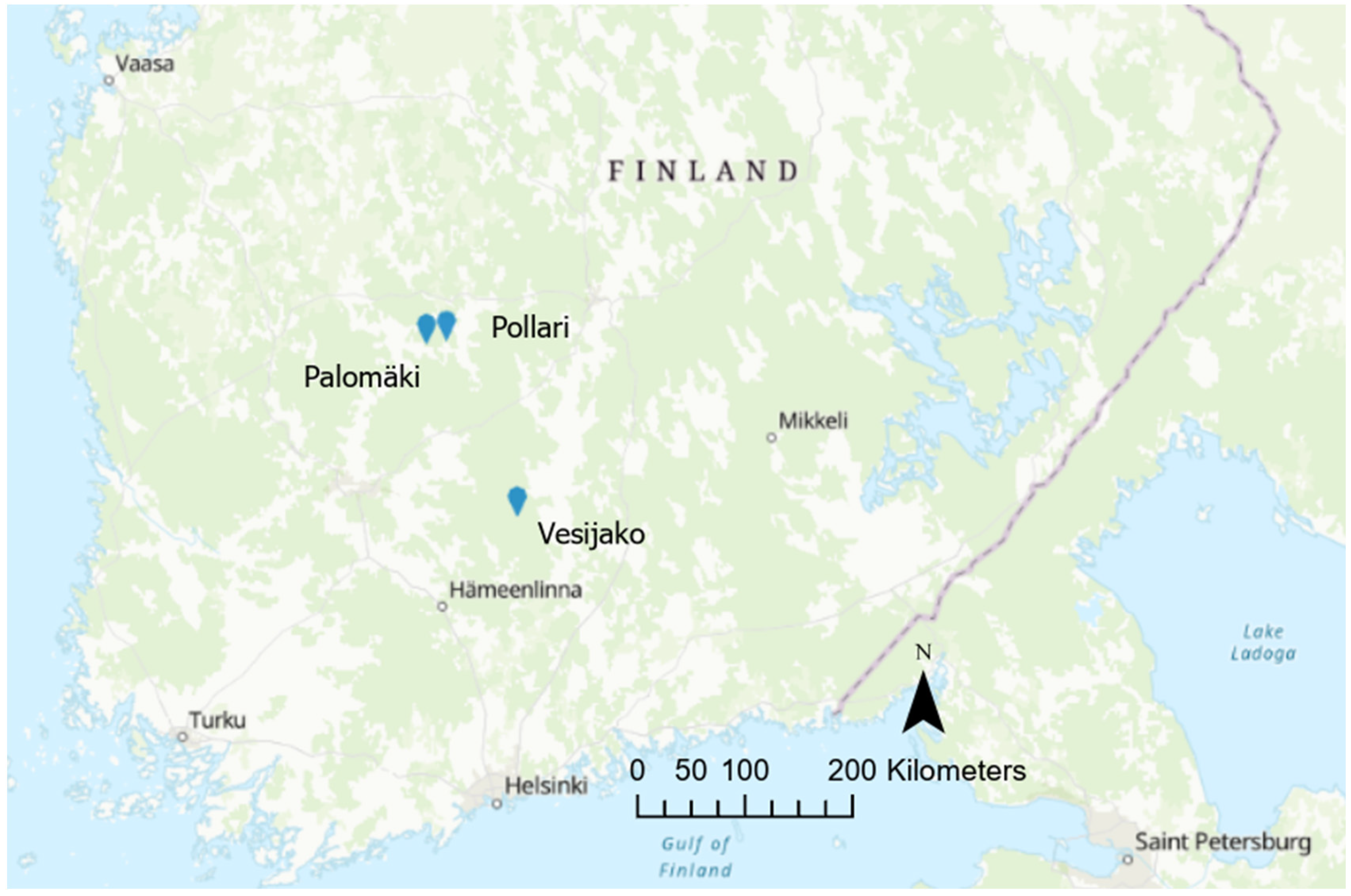
2.1. Study Area
2.2. Point Cloud Data Acquisition
2.3. Methods
3. Results
3.1. Tree Detection
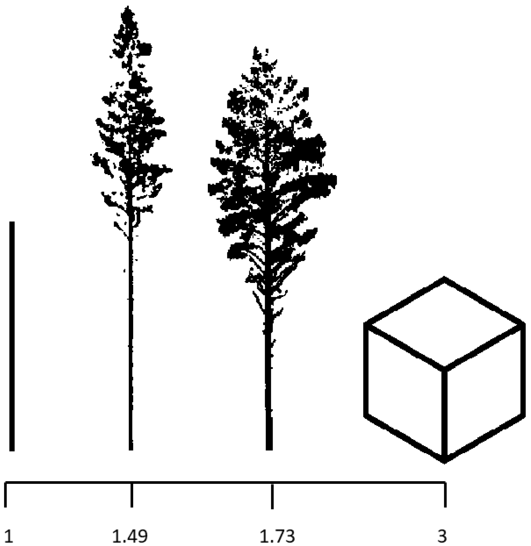
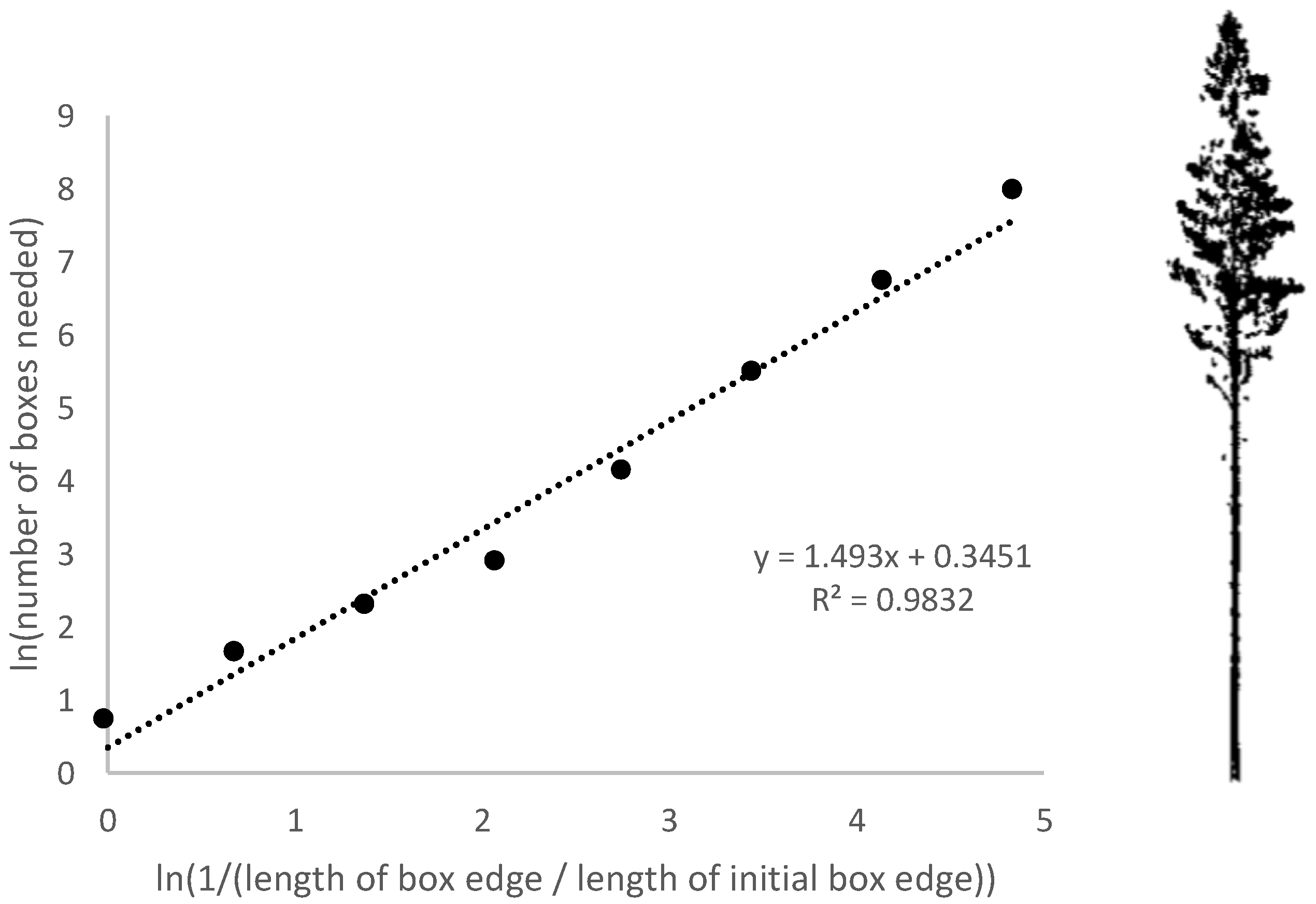
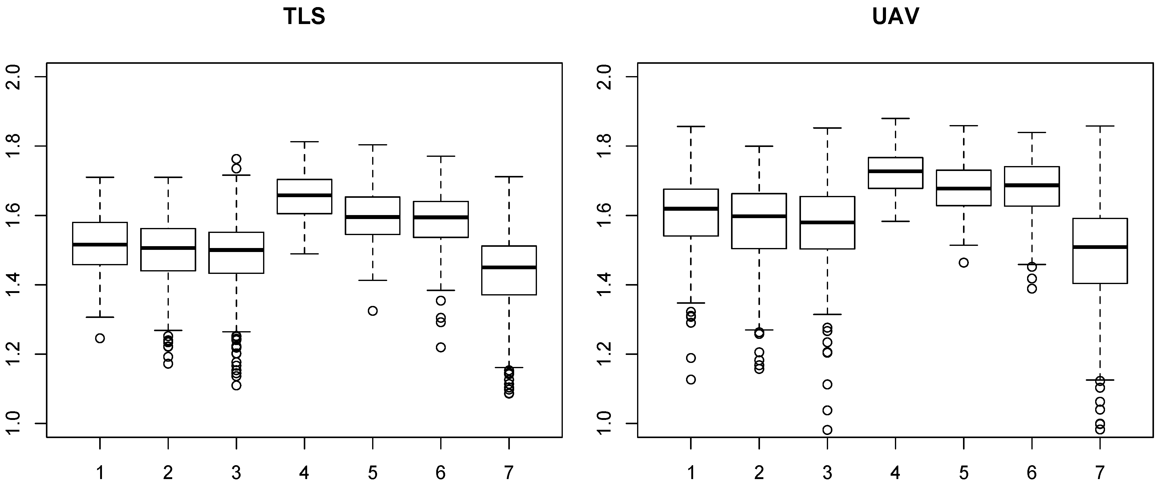
3.2. Box Dimension Values
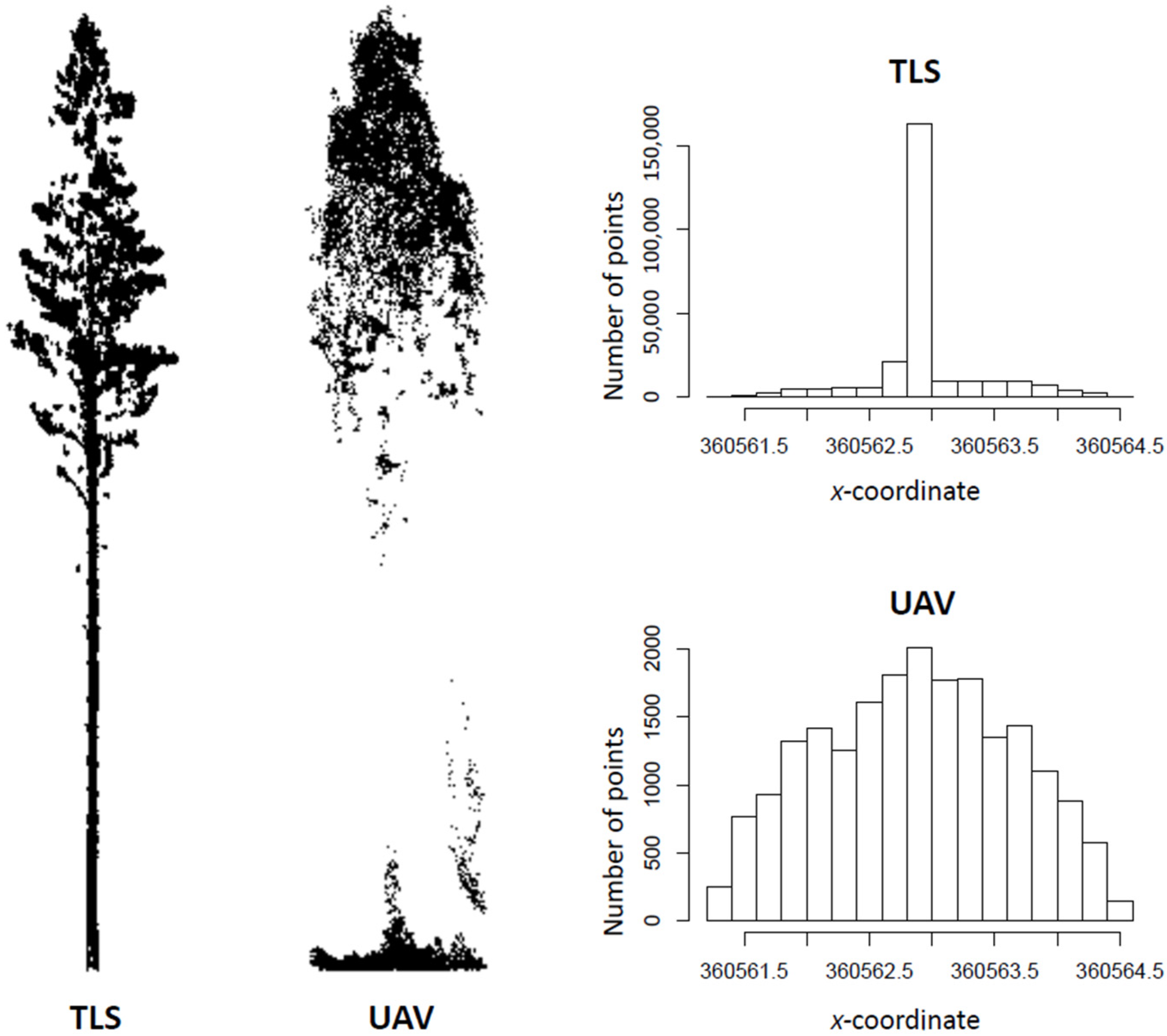
3.3. Number and Distribution of Points
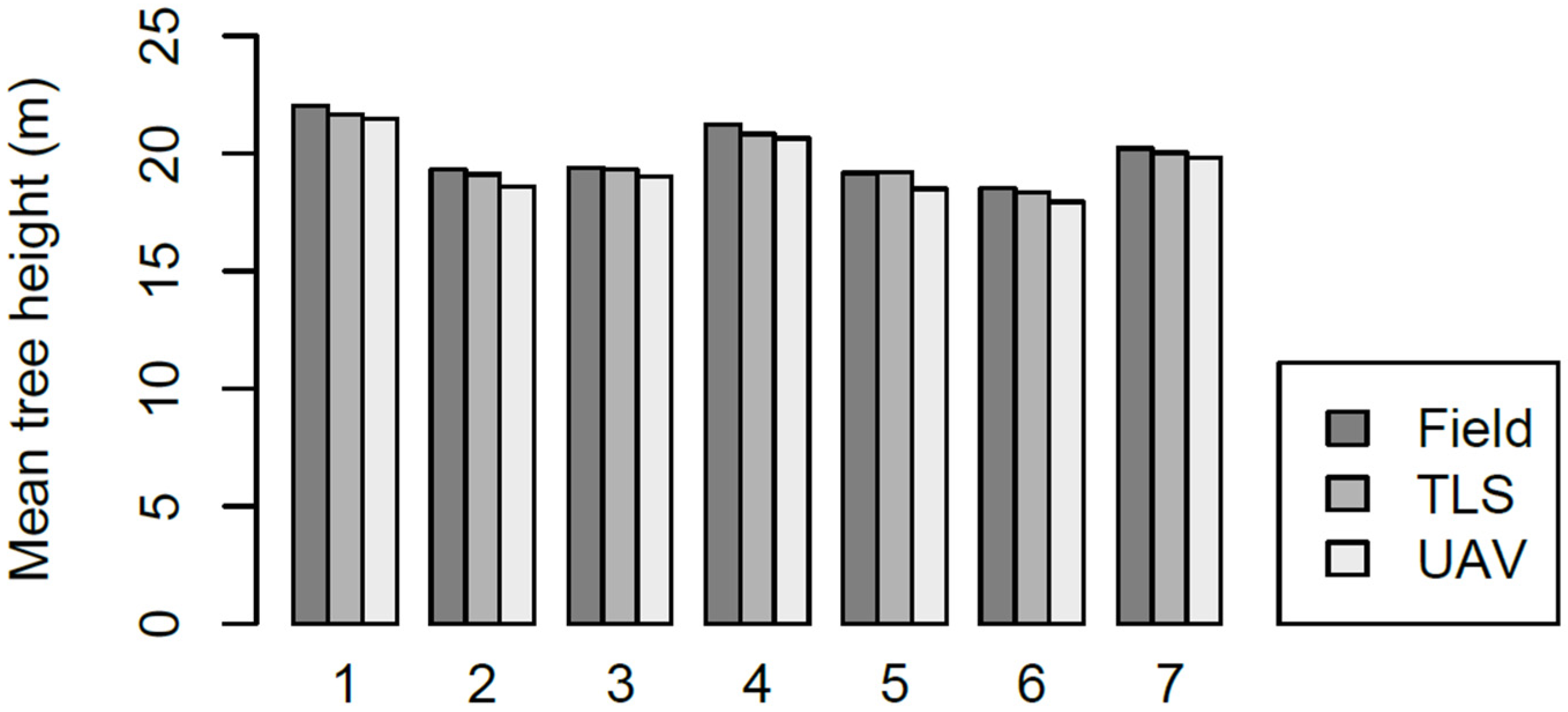
3.4. Tree Heights and Number of Boxes
4. Discussion
4.1. Tree Detection
4.2. Box Dimension Values
4.3. Number and Distribution of Points
4.4. Tree Heights and Number of Boxes
4.5. Limitations and Future Work
5. Conclusions
Author Contributions
Funding
Conflicts of Interest
References
- Juchheim, J.; Ehbrecht, M.; Schall, P.; Ammer, C.; Seidel, D. Effect of Tree Species Mixing on Stand Structural Complexity. Forestry 2020, 93, 75–83. [Google Scholar] [CrossRef]
- Seidel, D.; Ehbrecht, M.; Dorji, Y.; Jambay, J.; Ammer, C.; Annighöfer, P. Identifying Architectural Characteristics That Determine Tree Structural Complexity. Trees Struct. Funct. 2019, 33, 911–919. [Google Scholar] [CrossRef]
- Saarinen, N.; Kankare, V.; Yrttimaa, T.; Viljanen, N.; Honkavaara, E.; Holopainen, M.; Hyyppä, J.; Huuskonen, S.; Hynynen, J.; Vastaranta, M. Assessing the Effects of Thinning on Stem Growth Allocation of Individual Scots Pine Trees. For. Ecol. Manag. 2020, 474, 118344. [Google Scholar] [CrossRef]
- Saarinen, N.; Calders, K.; Kankare, V.; Yrttimaa, T.; Junttila, S.; Luoma, V.; Huuskonen, S.; Hynynen, J.; Verbeeck, H. Understanding 3D Structural Complexity of Individual Scots Pine Trees with Different Management History. Ecol. Evol. 2021, 11, 2561–2572. [Google Scholar] [CrossRef] [PubMed]
- Seidel, D.; Annighöfer, P.; Ehbrecht, M.; Magdon, P.; Wöllauer, S.; Ammer, C. Deriving Stand Structural Complexity from Airborne Laser Scanning Data—What Does It Tell Us about a Forest? Remote Sens. 2020, 12, 1854. [Google Scholar] [CrossRef]
- Pommerening, A. Approaches to Quantifying Forest Structures. For. Int. J. For. Res. 2002, 75, 305–324. [Google Scholar] [CrossRef]
- Ribe, R.G. In-Stand Scenic Beauty of Variable Retention Harvests and Mature Forests in the U.S. Pacific Northwest: The Effects of Basal Area, Density, Retention Pattern and down Wood. J. Environ. Manag. 2009, 91, 245–260. [Google Scholar] [CrossRef]
- Ehbrecht, M.; Schall, P.; Ammer, C.; Seidel, D. Quantifying Stand Structural Complexity and Its Relationship with Forest Management, Tree Species Diversity and Microclimate. Agric. For. Meteorol. 2017, 242, 1–9. [Google Scholar] [CrossRef]
- Gough, C.M.; Atkins, J.W.; Fahey, R.T.; Hardiman, B.S. High Rates of Primary Production in Structurally Complex Forests. Ecology 2019, 100, e02864. [Google Scholar] [CrossRef]
- Hardiman, B.S.; Gough, C.M.; Halperin, A.; Hofmeister, K.L.; Nave, L.E.; Bohrer, G.; Curtis, P.S. Maintaining High Rates of Carbon Storage in Old Forests: A Mechanism Linking Canopy Structure to Forest Function. For. Ecol. Manag. 2013, 298, 111–119. [Google Scholar] [CrossRef]
- Jayathunga, S.; Owari, T.; Tsuyuki, S. Analysis of Forest Structural Complexity Using Airborne LiDAR Data and Aerial Photography in a Mixed Conifer–Broadleaf Forest in Northern Japan. J. For. Res. 2018, 29, 479–493. [Google Scholar] [CrossRef]
- Zenner, E.K.; Hibbs, D.E. A New Method for Modeling the Heterogeneity of Forest Structure. For. Ecol. Manag. 2000, 129, 75–87. [Google Scholar] [CrossRef]
- Füldner, K. Zur Strukturbeschreibung in Mischbeständen. Forstarchiv 1995, 66, 235–240. [Google Scholar]
- Seidel, D.; Ehbrecht, M.; Puettmann, K. Assessing Different Components of Three-Dimensional Forest Structure with Single-Scan Terrestrial Laser Scanning: A Case Study. For. Ecol. Manag. 2016, 381, 196–208. [Google Scholar] [CrossRef]
- Newnham, G.J.; Armston, J.D.; Calders, K.; Disney, M.I.; Lovell, J.L.; Schaaf, C.B.; Strahler, A.H.; Mark Danson, F. Terrestrial Laser Scanning for Plot-Scale Forest Measurement. Curr. For. Rep. 2015, 1, 239–251. [Google Scholar] [CrossRef]
- Brede, B.; Lau, A.; Bartholomeus, H.M.; Kooistra, L. Comparing RIEGL RiCOPTER UAV LiDAR Derived Canopy Height and DBH with Terrestrial LiDAR. Sensors 2017, 17, 2371. [Google Scholar] [CrossRef]
- Atkins, J.W.; Bohrer, G.; Fahey, R.T.; Hardiman, B.S.; Morin, T.H.; Stovall, A.E.L.; Zimmerman, N.; Gough, C.M. Quantifying Vegetation and Canopy Structural Complexity from Terrestrial LiDAR Data Using the Forestr r Package. Methods Ecol. Evol. 2018, 9, 2057–2066. [Google Scholar] [CrossRef]
- Reich, K.F.; Kunz, M.; von Oheimb, G. A New Index of Forest Structural Heterogeneity Using Tree Architectural Attributes Measured by Terrestrial Laser Scanning. Ecol. Indic. 2021, 133, 108412. [Google Scholar] [CrossRef]
- Liang, X.; Kankare, V.; Hyyppä, J.; Wang, Y.; Kukko, A.; Haggrén, H.; Yu, X.; Kaartinen, H.; Jaakkola, A.; Guan, F.; et al. Terrestrial Laser Scanning in Forest Inventories. ISPRS J. Photogramm. Remote Sens. 2016, 115, 63–77. [Google Scholar] [CrossRef]
- Westoby, M.J.; Brasington, J.; Glasser, N.F.; Hambrey, M.J.; Reynolds, J.M. ‘Structure-from-Motion’ Photogrammetry: A Low-Cost, Effective Tool for Geoscience Applications. Geomorphology 2012, 179, 300–314. [Google Scholar] [CrossRef]
- Johnson, K.; Nissen, E.; Saripalli, S.; Arrowsmith, J.R.; McGarey, P.; Scharer, K.; Williams, P.; Blisniuk, K. Rapid Mapping of Ultrafine Fault Zone Topography with Structure from Motion. Geosphere 2014, 10, 969–986. [Google Scholar] [CrossRef]
- Alexiou, S.; Deligiannakis, G.; Pallikarakis, A.; Papanikolaou, I.; Psomiadis, E.; Reicherter, K. Comparing High Accuracy T-LiDAR and UAV-SfM Derived Point Clouds for Geomorphological Change Detection. ISPRS Int. J. Geo-Inf. 2021, 10, 367. [Google Scholar] [CrossRef]
- Aicardi, I.; Dabove, P.; Lingua, A.M.; Piras, M. Integration between TLS and UAV Photogrammetry Techniques for Forestry Applications. Iforest Biogeosci. For. 2016, 10, 41. [Google Scholar] [CrossRef]
- Son, S.W.; Kim, D.W.; Sung, W.G.; Yu, J.J. Integrating UAV and TLS Approaches for Environmental Management: A Case Study of a Waste Stockpile Area. Remote Sens. 2020, 12, 1615. [Google Scholar] [CrossRef]
- Garcia, G.P.B.; Gomes, E.B.; Viana, C.D.; Grohmann, C.H. Comparing Terrestrial Laser Scanner and UAV-Based Photogrammetry to Generate a Landslide DEM. In Proceedings of the XIX Brazilian Symposium on Remote Sensing, Santos, Brazil, 14–17 April 2019; pp. 415–418. [Google Scholar]
- Wilkes, P.; Lau, A.; Disney, M.; Calders, K.; Burt, A.; Gonzalez de Tanago, J.; Bartholomeus, H.; Brede, B.; Herold, M. Data Acquisition Considerations for Terrestrial Laser Scanning of Forest Plots. Remote Sens. Environ. 2017, 196, 140–153. [Google Scholar] [CrossRef]
- van Leeuwen, M.; Nieuwenhuis, M. Retrieval of Forest Structural Parameters Using LiDAR Remote Sensing. Eur. J. For. Res. 2010, 129, 749–770. [Google Scholar] [CrossRef]
- Yrttimaa, T.; Saarinen, N.; Kankare, V.; Viljanen, N.; Hynynen, J.; Huuskonen, S.; Holopainen, M.; Hyyppä, J.; Honkavaara, E.; Vastaranta, M. Multisensorial Close-Range Sensing Generates Benefits for Characterization of Managed Scots Pine (Pinus sylvestris L.) Stands. ISPRS Int. J. Geo-Inf. 2020, 9, 309. [Google Scholar] [CrossRef]
- White, J.C.; Wulder, M.A.; Vastaranta, M.; Coops, N.C.; Pitt, D.; Woods, M. The Utility of Image-Based Point Clouds for Forest Inventory: A Comparison with Airborne Laser Scanning. Forests 2013, 4, 518–536. [Google Scholar] [CrossRef]
- Wallace, L.; Lucieer, A.; Malenovskỳ, Z.; Turner, D.; Vopěnka, P. Assessment of Forest Structure Using Two UAV Techniques: A Comparison of Airborne Laser Scanning and Structure from Motion (SfM) Point Clouds. Forests 2016, 7, 62. [Google Scholar] [CrossRef]
- Mandelbrot, B.B. The Fractal Geometry of Nature; W.H. Freeman Company: New York, NY, USA, 1977. [Google Scholar]
- Seidel, D. A Holistic Approach to Determine Tree Structural Complexity Based on Laser Scanning Data and Fractal Analysis. Ecol. Evol. 2018, 8, 128–134. [Google Scholar] [CrossRef]
- Feldman, D.P. Chaos and Fractals. An Elementary Introduction; Oxford University Press: Oxford, UK, 2012; ISBN 9780199566440. [Google Scholar]
- Dorji, Y.; Annighöfer, P.; Ammer, C.; Seidel, D. Response of Beech (Fagus sylvatica L.) Trees to Competition—New Insights from Using Fractal Analysis. Remote Sens. 2019, 11, 2656. [Google Scholar] [CrossRef]
- Seidel, D.; Annighöfer, P.; Stiers, M.; Zemp, C.D.; Burkardt, K.; Ehbrecht, M.; Willim, K.; Kreft, H.; Hölscher, D.; Ammer, C. How a Measure of Tree Structural Complexity Relates to Architectural Benefit-to-Cost Ratio, Light Availability, and Growth of Trees. Ecol. Evol. 2019, 9, 7134–7142. [Google Scholar] [CrossRef] [PubMed]
- Arseniou, G.; Macfarlane, D.W.; Seidel, D. Measuring the Contribution of Leaves to the Structural Complexity of Urban Tree Crowns with Terrestrial Laser Scanning. Remote Sens. 2021, 13, 2773. [Google Scholar] [CrossRef]
- Arseniou, G.; Macfarlane, D.W.; Seidel, D. Woody Surface Area Measurements with Terrestrial Laser Scanning Relate to the Anatomical and Structural Complexity of Urban Trees. Remote Sens. 2021, 13, 3153. [Google Scholar] [CrossRef]
- Yrttimaa, T.; Saarinen, N.; Kankare, V.; Hynynen, J.; Huuskonen, S.; Holopainen, M.; Hyyppä, J.; Vastaranta, M. Performance of Terrestrial Laser Scanning to Characterize Managed Scots Pine (Pinus sylvestris L.) Stands Is Dependent on Forest Structural Variation. ISPRS J. Photogramm. Remote Sens. 2020, 168, 277–287. [Google Scholar] [CrossRef]
- Finnish Forestry Practice and Management; Rantala, S. (Ed.) Metsäkustannus: Helsinki, Finland, 2011. [Google Scholar]
- James, M.R.; Robson, S. Mitigating Systematic Error in Topographic Models Derived from UAV and Ground-Based Image Networks. Earth Surf. Process. Landf. 2014, 39, 1413–1420. [Google Scholar] [CrossRef]
- Cunliffe, A.M.; Brazier, R.E.; Anderson, K. Ultra-Fine Grain Landscape-Scale Quantification of Dryland Vegetation Structure with Drone-Acquired Structure-from-Motion Photogrammetry. Remote Sens. Environ. 2016, 183, 129–143. [Google Scholar] [CrossRef]
- Viljanen, N.; Honkavaara, E.; Näsi, R.; Hakala, T.; Niemeläinen, O.; Kaivosoja, J. A Novel Machine Learning Method for Estimating Biomass of Grass Swards Using a Photogrammetric Canopy Height Model, Images and Vegetation Indices Captured by a Drone. Agriculture 2018, 8, 70. [Google Scholar] [CrossRef]
- Puliti, S.; Ørka, H.O.; Gobakken, T.; Næsset, E. Inventory of Small Forest Areas Using an Unmanned Aerial System. Remote Sens. 2015, 7, 9632–9654. [Google Scholar] [CrossRef]
- Isenburg, M. LAStools—Efficient LiDAR Processing Software (Version 181001 Academic) | Rapidlasso GmbH. Available online: https://rapidlasso.com/lastools/ (accessed on 18 July 2022).
- Ritter, T.; Schwarz, M.; Tockner, A.; Leisch, F.; Nothdurft, A. Automatic Mapping of Forest Stands Based on Three-Dimensional Point Clouds Derived from Terrestrial Laser-Scanning. Forests 2017, 8, 265. [Google Scholar] [CrossRef]
- Popescu, S.C.; Wynne, R.H. Seeing the Trees in the Forest: Using Lidar and Multispectral Data Fusion with Local Filtering and Variable Window Size for Estimating Tree Height. Photogramm. Eng. Remote Sens. 2004, 70, 589–604. [Google Scholar] [CrossRef]
- Meyer, F.; Beucher, S. Morphological Segmentation. J. Vis. Commun. Image Represent. 1990, 1, 21–46. [Google Scholar] [CrossRef]
- Plowright, A.; Roussel, J.-R. ForestTools: Analyzing Remotely Sensed Forest Data. R Package Version 0.2.5. Available online: https://cran.r-project.org/package=ForestTools (accessed on 11 August 2022).
- Juchheim, J.; Annighöfer, P.; Ammer, C.; Calders, K.; Raumonen, P.; Seidel, D. How Management Intensity and Neighborhood Composition Affect the Structure of Beech (Fagus sylvatica L.) Trees. Trees 2017, 31, 1723–1735. [Google Scholar] [CrossRef]
- Li, Q.; Ma, Y.; Anderson, J.; Curry, J.; Shan, J. Towards Uniform Point Density: Evaluation of an Adaptive Terrestrial Laser Scanner. Remote Sens. 2019, 11, 880. [Google Scholar] [CrossRef]
- Wilkinson, M.W.; Jones, R.R.; Woods, C.E.; Gilment, S.R.; McCaffrey, K.J.W.; Kokkalas, S.; Long, J.J. A Comparison of Terrestrial Laser Scanning and Structure-from-Motion Photogrammetry as Methods for Digital Outcrop Acquisition. Geosphere 2016, 12, 1865–1880. [Google Scholar] [CrossRef]
- Kameyama, S.; Sugiura, K. Estimating Tree Height and Volume Using Unmanned Aerial Vehicle Photography and SfM Technology, with Verification of Result Accuracy. Drones 2020, 4, 19. [Google Scholar] [CrossRef]
- Krooks, A.; Kaasalainen, S.; Kankare, V.; Joensuu, M.; Raumonen, P.; Kaasalainen, M. Predicting Tree Structure from Tree Height Using Terrestrial Laser Scanning and Quantitative Structure Models. Silva Fenn. 2014, 48, 1125. [Google Scholar] [CrossRef]
- Vaglio Laurin, G.; Ding, J.; Disney, M.; Bartholomeus, H.; Herold, M.; Papale, D.; Valentini, R. Tree Height in Tropical Forest as Measured by Different Ground, Proximal, and Remote Sensing Instruments, and Impacts on above Ground Biomass Estimates. Int. J. Appl. Earth Obs. Geoinf. 2019, 82, 101899. [Google Scholar] [CrossRef]
- Winczek, M.; Zięba-Kulawik, K.; Wężyk, P.; Strejczek-Jaźwińska, P.; Bobrowski, R.; Szparadowska, M.; Warchoł, A.; Kiedos, D. LiDAR and Image Point Clouds as a Source of 3D Information for a Smart City-the Case Study for Trees in Jordan Park in Kraków, Poland. In Proceedings of the Symposium GIS Ostrava 2020—UAV in Smart City and Smart Region, Ostrava, Czech Republic, 18–20 March 2020; Kačmařík, M., Růžička, J., Eds.; Available online: http://gisak.vsb.cz/GIS_Ostrava/GIS_Ova_2020/proceedings/papers/gis20205e3c1766d2e87.pdf (accessed on 11 August 2022).
- Roşca, S.; Suomalainen, J.; Bartholomeus, H.; Herold, M. Comparing Terrestrial Laser Scanning and Unmanned Aerial Vehicle Structure from Motion to Assess Top of Canopy Structure in Tropical Forests. Interface Focus 2018, 8, 20170038. [Google Scholar] [CrossRef]
- Brede, B.; Calders, K.; Lau, A.; Raumonen, P.; Bartholomeus, H.M.; Herold, M.; Kooistra, L. Non-Destructive Tree Volume Estimation through Quantitative Structure Modelling: Comparing UAV Laser Scanning with Terrestrial LIDAR. Remote Sens. Environ. 2019, 233, 111355. [Google Scholar] [CrossRef]
- Liang, X.; Wang, Y.; Pyörälä, J.; Lehtomäki, M.; Yu, X.; Kaartinen, H.; Kukko, A.; Honkavaara, E.; Issaoui, A.E.I.; Nevalainen, O.; et al. Forest in Situ Observations Using Unmanned Aerial Vehicle as an Alternative of Terrestrial Measurements. Ecosyst 2019, 6, 20. [Google Scholar] [CrossRef]
- Puliti, S.; Breidenbach, J.; Astrup, R. Estimation of Forest Growing Stock Volume with UAV Laser Scanning Data: Can It Be Done without Field Data? Remote Sens. 2020, 12, 1245. [Google Scholar] [CrossRef]
- Terryn, L.; Calders, K.; Bartholomeus, H.; Bartolo, R.E.; Brede, B.; D’hont, B.; Disney, M.; Herold, M.; Lau, A.; Shenkin, A.; et al. Quantifying Tropical Forest Structure through Terrestrial and UAV Laser Scanning Fusion in Australian Rainforests. Remote Sens. Environ. 2022, 271, 112912. [Google Scholar] [CrossRef]
- Jaakkola, A.; Hyyppä, J.; Kukko, A.; Yu, X.; Kaartinen, H.; Lehtomäki, M.; Lin, Y. A Low-Cost Multi-Sensoral Mobile Mapping System and Its Feasibility for Tree Measurements. ISPRS J. Photogramm. Remote Sens. 2010, 65, 514–522. [Google Scholar] [CrossRef]
- Jaakkola, A.; Hyyppä, J.; Yu, X.; Kukko, A.; Kaartinen, H.; Liang, X.; Hyyppä, H.; Wang, Y. Autonomous Collection of Forest Field Reference—The Outlook and a First Step with UAV Laser Scanning. Remote Sens. 2017, 9, 785. [Google Scholar] [CrossRef]
- Mokroš, M.; Liang, X.; Surový, P.; Valent, P.; Čerňava, J.; Chudý, F.; Tunák, D.; Saloň, I.; Merganič, J. Evaluation of Close-Range Photogrammetry Image Collection Methods for Estimating Tree Diameters. ISPRS Int. J. Geo-Inf. 2018, 7, 93. [Google Scholar] [CrossRef]
- Hunčaga, M.; Chudá, J.; Tomaštík, J.; Slámová, M.; Koreň, M.; Chudý, F. The Comparison of Stem Curve Accuracy Determined from Point Clouds Acquired by Different Terrestrial Remote Sensing Methods. Remote Sens. 2020, 12, 2739. [Google Scholar] [CrossRef]
- Morsdorf, F.; Kükenbrink, D.; Schneider, F.D.; Abegg, M.; Schaepman, M.E. Close-Range Laser Scanning in Forests: Towards Physically Based Semantics across Scales. Interface Focus 2018, 8, 20170046. [Google Scholar] [CrossRef]


| Palomäki | Pollari | Vesijako | |
|---|---|---|---|
| Coordinates | 62°3.6′ N 24°19.9′ E | 62°4.4′ N 24°30.1′ E | 61°21.8′ N 25°6.3′ E |
| Municipality | Mänttä-Vilppula | Mänttä-Vilppula | Padasjoki |
| Elevation above sea level (m) | 135 | 155 | 120 |
| Temperature sum (° days) | 1195 | 1130 | 1256 |
| Year of establishment | 2005 | 2006 | 2006 |
| Age at establishment | 50 | 45 | 59 |
| Thinning treatments | 2006 | 2006 | 2007 |
| The latest field measurements | April 2019 | October 2018 | April 2019 |
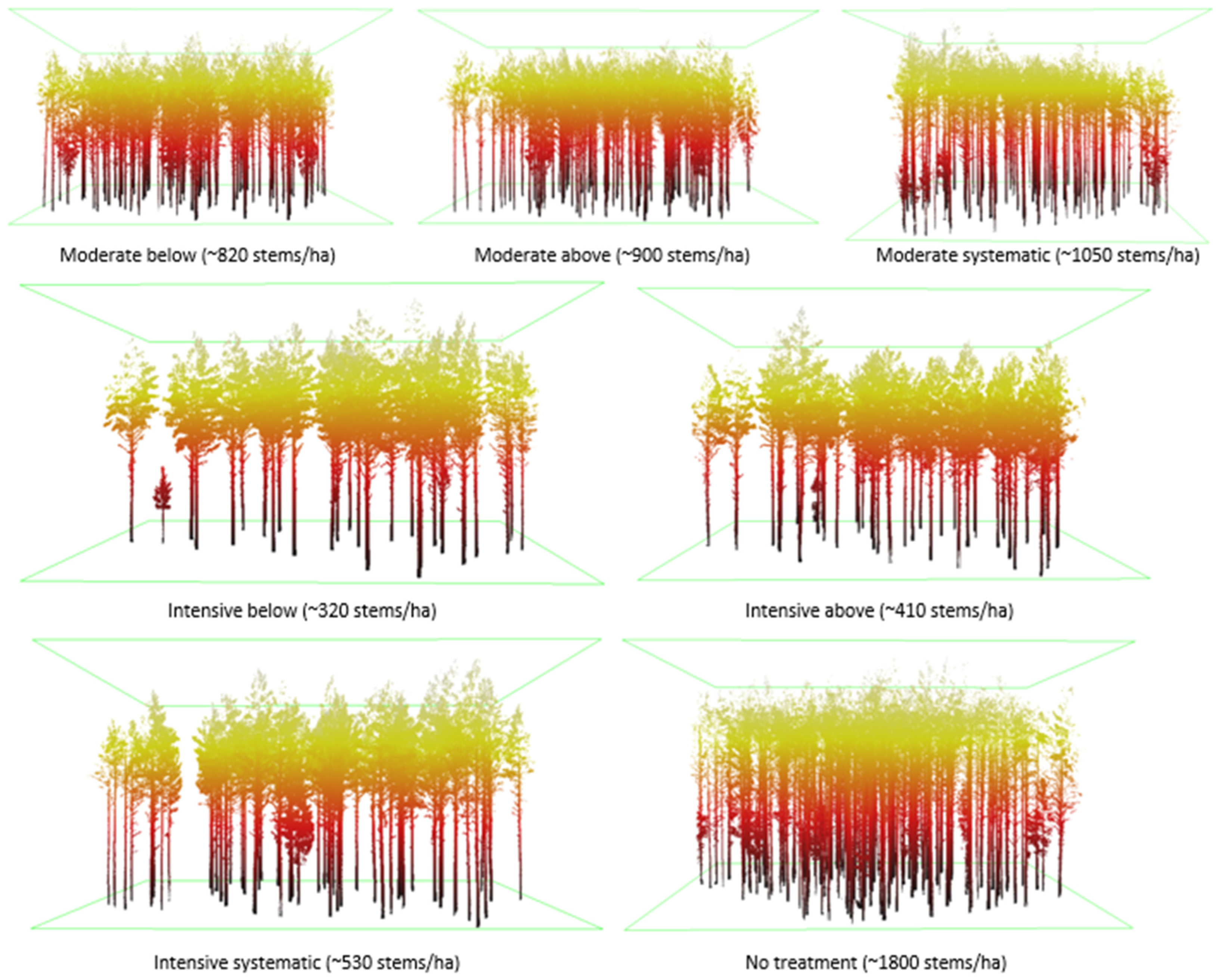
| Thinning Treatment | Number | Explanation | Number of Plots |
|---|---|---|---|
| Moderate thinning from below | 1 | Moderate thinning refers to prevailing thinning guidelines applied in Finland [39]. | 3 |
| Moderate thinning from above | 2 | 4 | |
| Moderate systematic thinning | 3 | 5 | |
| Intensive thinning from below | 4 | Intensive thinning corresponds 50% lower remaining basal area (m2/ha) than in the plots with moderate thinning intensity. | 3 |
| Intensive thinning from above | 5 | 4 | |
| Intensive systematic thinning | 6 | 5 | |
| Control/no treatment | 7 | No thinning treatment since the establishment. | 3 (27 in total) |
| Study Site | RMSEs of GCPs (cm) | ||
|---|---|---|---|
| x | y | z | |
| Palomäki | 0.64 | 1.36 | 0.68 |
| Pollari | 0.48 | 0.47 | 0.29 |
| Vesijako | 1.25 | 1.75 | 1.19 |
| Data Acquisition | Point Cloud Generation | Height- Normalization | Co-Registration | Tree Segmentation | Box Dimension |
|---|---|---|---|---|---|
| Multi-scan TLS | Co-registration of individual scans: FARO SCENE software | LAStools (lasground) | 3D rigid transformation from the scanner CRS (TLS) to global CRS (UAV) based on manually extracted tie points: MATLAB | 1. CHM generation: LAStools (lascanopy); 2. Variable window filtering to detect treetops: R, ForestTools [48] 3. Marker-controlled watershed segmentation to segment tree crowns: R, ForestTools; 4. Point-in-polygon approach to extract tree point clouds: LAStools | Assessment of tree structural complexity using box dimension: R |
| UAV photogrammetry | Photogrammetric processing: Agisoft Metashape Quality setting: ‘high’ Depth filtering: ‘mild’ | Open-source DTM + LAStools (lasheight) |
| Treatment | Number | Trees/ha | Undetected Scots Pines | Detection Rate (%) | ||
|---|---|---|---|---|---|---|
| TLS | UAV | TLS | UAV | |||
| Moderate below | 1 | 712 | 1 | 3 | 99.6 | 98.7 |
| Moderate above | 2 | 924 | 2 | 2 | 99.5 | 99.5 |
| Moderate systematic | 3 | 958 | 11 | 15 | 97.8 | 97.0 |
| Intensive below | 4 | 286 | 0 | 0 | 100.0 | 100.0 |
| Intensive above | 5 | 450 | 3 | 3 | 98.5 | 98.5 |
| Intensive systematic | 6 | 473 | 3 | 4 | 98.9 | 98.5 |
| No treatment | 7 | 1315 | 12 | 15 | 97.1 | 96.3 |
| All plots | 727 | 32 | 42 | 98.5 | 98.0 | |
| Treatment | Mean | Minimum | Maximum | Range | ||||
|---|---|---|---|---|---|---|---|---|
| TLS | UAV | TLS | UAV | TLS | UAV | TLS | UAV | |
| Moderate below | 1.51 ± 0.10 | 1.59 ± 0.17 | 0.81 | 0.34 | 1.71 | 1.86 | 0.90 | 1.51 |
| Moderate above | 1.50 ± 0.09 | 1.57 ± 0.12 | 1.17 | 1.16 | 1.71 | 1.80 | 0.54 | 0.64 |
| Moderate systematic | 1.49 ± 0.10 | 1.57 ± 0.14 | 1.11 | 0.23 | 1.76 | 1.85 | 0.65 | 1.62 |
| Intensive below | 1.65 ± 0.06 | 1.72 ± 0.07 | 1.49 | 1.58 | 1.81 | 1.88 | 0.32 | 0.30 |
| Intensive above | 1.60 ± 0.08 | 1.68 ± 0.07 | 1.32 | 1.46 | 1.80 | 1.86 | 0.48 | 0.39 |
| Intensive systematic | 1.59 ± 0.08 | 1.68 ± 0.08 | 1.22 | 1.39 | 1.77 | 1.84 | 0.55 | 0.45 |
| No treatment | 1.43 ± 0.11 | 1.49 ± 0.16 | 1.09 | 0.48 | 1.71 | 1.86 | 0.63 | 1.38 |
| All plots | 1.51 ± 0.11 | 1.59 ± 0.15 | 0.81 | 0.23 | 1.81 | 1.88 | 1.01 | 1.65 |
| Treatment | TLS | UAV | ||
|---|---|---|---|---|
| Db | Points (in K) | Db | Points (in K) | |
| Moderate below | 1.51 | 515 ± 318 | 1.59 | 36 ± 18 |
| Moderate above | 1.50 | 460 ± 286 | 1.57 | 27 ± 17 |
| Moderate systematic | 1.49 | 428 ± 290 | 1.57 | 28 ± 15 |
| Intensive below | 1.65 | 912 ± 435 | 1.72 | 70 ± 22 |
| Intensive above | 1.60 | 615 ± 308 | 1.68 | 39 ± 17 |
| Intensive systematic | 1.59 | 577 ± 348 | 1.68 | 42 ± 17 |
| No treatment | 1.43 | 384 ± 282 | 1.49 | 19 ± 12 |
| All plots | 1.51 | 494 ± 330 | 1.59 | 32 ± 20 |
| Number of UAV Points | Average Number of TLS Points | Db-TLS | Db-UAV | n |
|---|---|---|---|---|
| ≥80,000 | 1,149,000 | 1.68 | 1.77 | 39 |
| 80,000 > x ≥ 60,000 | 795,000 | 1.64 | 1.73 | 166 |
| 60,000 > x ≥ 40,000 | 626,000 | 1.58 | 1.69 | 385 |
| 40,000 > x ≥ 20,000 | 483,000 | 1.53 | 1.62 | 826 |
| 20,000 > x ≥ 0 | 315,000 | 1.41 | 1.44 | 649 |
| x ≥ 0 | 494,000 | 1.51 | 1.59 | 2065 |
| Treatment | TLS | UAV | ||
|---|---|---|---|---|
| Above (%) | Below (%) | Above (%) | Below (%) | |
| Moderate below | 30 | 70 | 83 | 17 |
| Moderate above | 34 | 66 | 82 | 18 |
| Moderate systematic | 32 | 68 | 81 | 19 |
| Intensive below | 44 | 56 | 69 | 31 |
| Intensive above | 44 | 56 | 72 | 28 |
| Intensive systematic | 42 | 58 | 72 | 28 |
| No treatment | 26 | 74 | 87 | 13 |
| All plots | 35 | 65 | 78 | 22 |
| Standard Deviation (cm) | Difference between Ranges, TLS–UAV (cm) | |||
|---|---|---|---|---|
| Axis | TLS | UAV | Difference | |
| x | 46 | 78 | 32 | 6 ± 15 |
| y | 46 | 78 | 32 | 6 ± 15 |
| z | 480 | 540 | 60 | 1 ± 191 |
| Mean Tree Height (m) | Mean Difference (m) | RMSE (m) | |||||
|---|---|---|---|---|---|---|---|
| Treatment | Field | TLS | UAV | Field–TLS | Field–UAV | TLS | UAV |
| Moderate below | 21.2 ± 2.1 | 20.8 ± 2.2 | 20.5 ± 2.3 | 0.43 | 0.68 | 1.47 | 1.55 |
| Moderate above | 20.4 ± 1.6 | 20.1 ± 1.7 | 19.9 ± 1.7 | 0.26 | 0.49 | 0.97 | 1.01 |
| Moderate systematic | 19.5 ± 2.1 | 19.4 ± 2.1 | 19.2 ± 2.1 | 0.18 | 0.31 | 1.54 | 1.49 |
| Intensive below | 21.3 ± 1.7 | 20.8 ± 1.9 | 20.7 ± 1.9 | 0.41 | 0.60 | 0.67 | 0.78 |
| Intensive above | 19.2 ± 1.5 | 18.9 ± 1.6 | 18.4 ± 1.6 | 0.28 | 0.72 | 0.77 | 0.97 |
| Intensive systematic | 18.9 ± 2.5 | 18.5 ± 2.5 | 18.3 ± 2.5 | 0.36 | 0.60 | 0.91 | 1.01 |
| No treatment | 20.4 ± 3.0 | 19.8 ± 2.8 | 19.8 ± 2.9 | 0.59 | 0.64 | 1.72 | 2.10 |
| All plots | 20.0 ± 2.3 | 19.7 ± 2.3 | 19.5 ± 2.4 | 0.34 | 0.54 | 1.32 | 1.44 |
| Average Number of Boxes | |||||
|---|---|---|---|---|---|
| Box Size | TLS | R2 | UAV | R2 | UAV > TLS |
| h | 2.6 | 0.01 | 2.7 | 0.00 | 4% |
| h/2 | 4.6 | 0.02 | 5.1 | 0.02 | 13% |
| h/4 | 9.5 | 0.19 | 11.7 | 0.19 | 23% |
| h/8 | 25.2 | 0.54 | 31.7 | 0.18 | 26% |
| h/16 | 82.5 | 0.71 | 106.8 | 0.71 | 29% |
| h/32 | 308.3 | 0.76 | 408.8 | 0.64 | 33% |
| h/64 | 1066.2 | 0.80 | 1566.6 | 0.68 | 47% |
| h/128 | 3293.3 | 0.79 | 5400.1 | 0.67 | 64% |
Publisher’s Note: MDPI stays neutral with regard to jurisdictional claims in published maps and institutional affiliations. |
© 2022 by the authors. Licensee MDPI, Basel, Switzerland. This article is an open access article distributed under the terms and conditions of the Creative Commons Attribution (CC BY) license (https://creativecommons.org/licenses/by/4.0/).
Share and Cite
Tienaho, N.; Yrttimaa, T.; Kankare, V.; Vastaranta, M.; Luoma, V.; Honkavaara, E.; Koivumäki, N.; Huuskonen, S.; Hynynen, J.; Holopainen, M.; et al. Assessing Structural Complexity of Individual Scots Pine Trees by Comparing Terrestrial Laser Scanning and Photogrammetric Point Clouds. Forests 2022, 13, 1305. https://doi.org/10.3390/f13081305
Tienaho N, Yrttimaa T, Kankare V, Vastaranta M, Luoma V, Honkavaara E, Koivumäki N, Huuskonen S, Hynynen J, Holopainen M, et al. Assessing Structural Complexity of Individual Scots Pine Trees by Comparing Terrestrial Laser Scanning and Photogrammetric Point Clouds. Forests. 2022; 13(8):1305. https://doi.org/10.3390/f13081305
Chicago/Turabian StyleTienaho, Noora, Tuomas Yrttimaa, Ville Kankare, Mikko Vastaranta, Ville Luoma, Eija Honkavaara, Niko Koivumäki, Saija Huuskonen, Jari Hynynen, Markus Holopainen, and et al. 2022. "Assessing Structural Complexity of Individual Scots Pine Trees by Comparing Terrestrial Laser Scanning and Photogrammetric Point Clouds" Forests 13, no. 8: 1305. https://doi.org/10.3390/f13081305