
Detecting Coastal Wetland Degradation by Combining Remote Sensing and Hydrologic Modeling


Abstract
:1. Introduction
2. Materials and Methods
2.1. Study Area
2.2. Data for Wetland Degradation Detection
2.2.1. Landsat Data
2.2.2. Landsat-Derived Normalized Difference Vegetation Index (NDVI)
2.2.3. Ancillary Datasets
2.3. Methodology
2.3.1. PIHM-Wetland Model
2.3.2. Data Used in the PIHM-Wetland Model
2.3.3. Model Setup
3. Results and Discussion
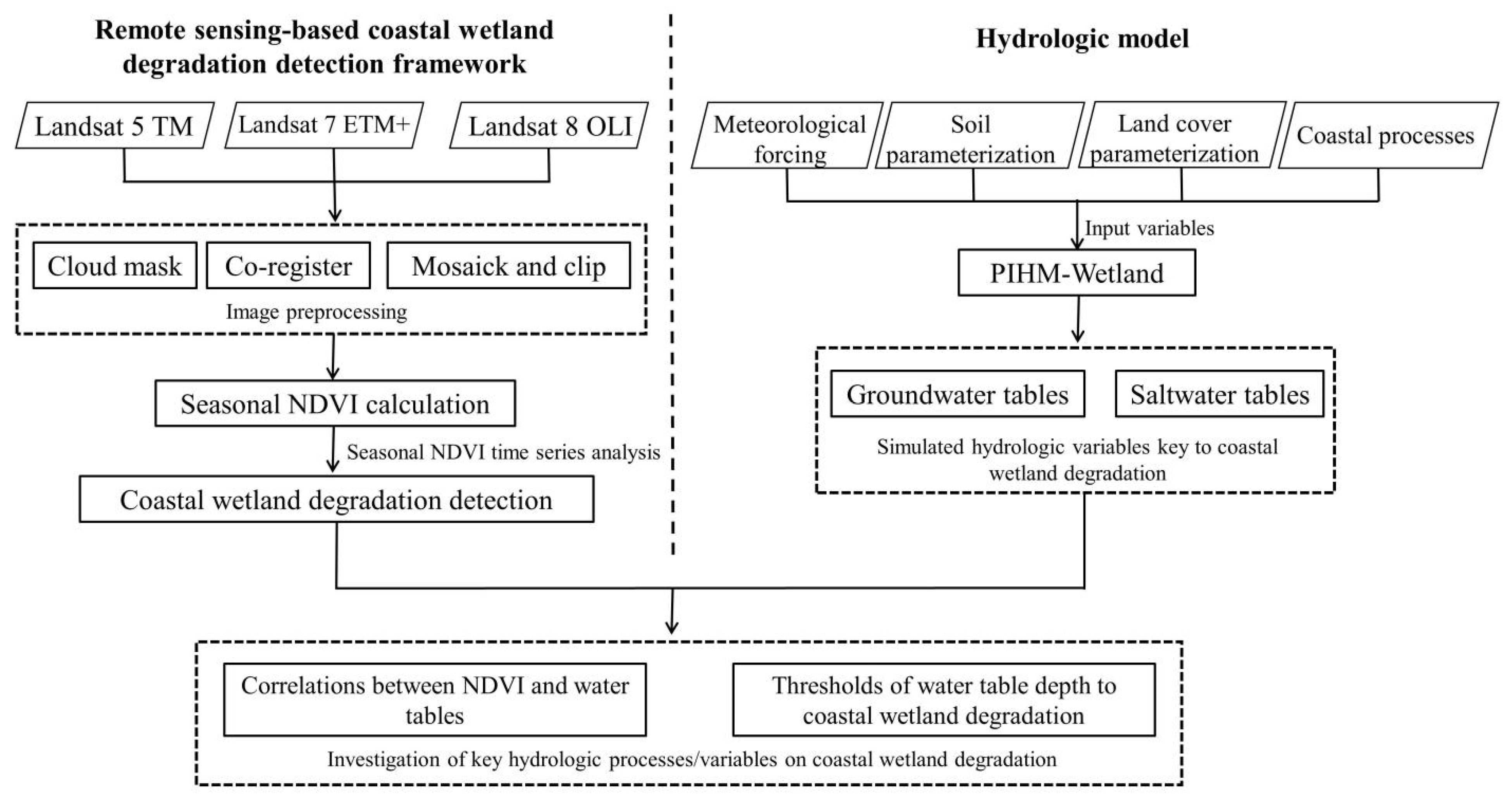
3.1. Framework to Detect Wetland Degradation
3.2. Wetland Degradation during the Period from 1995 to 2019
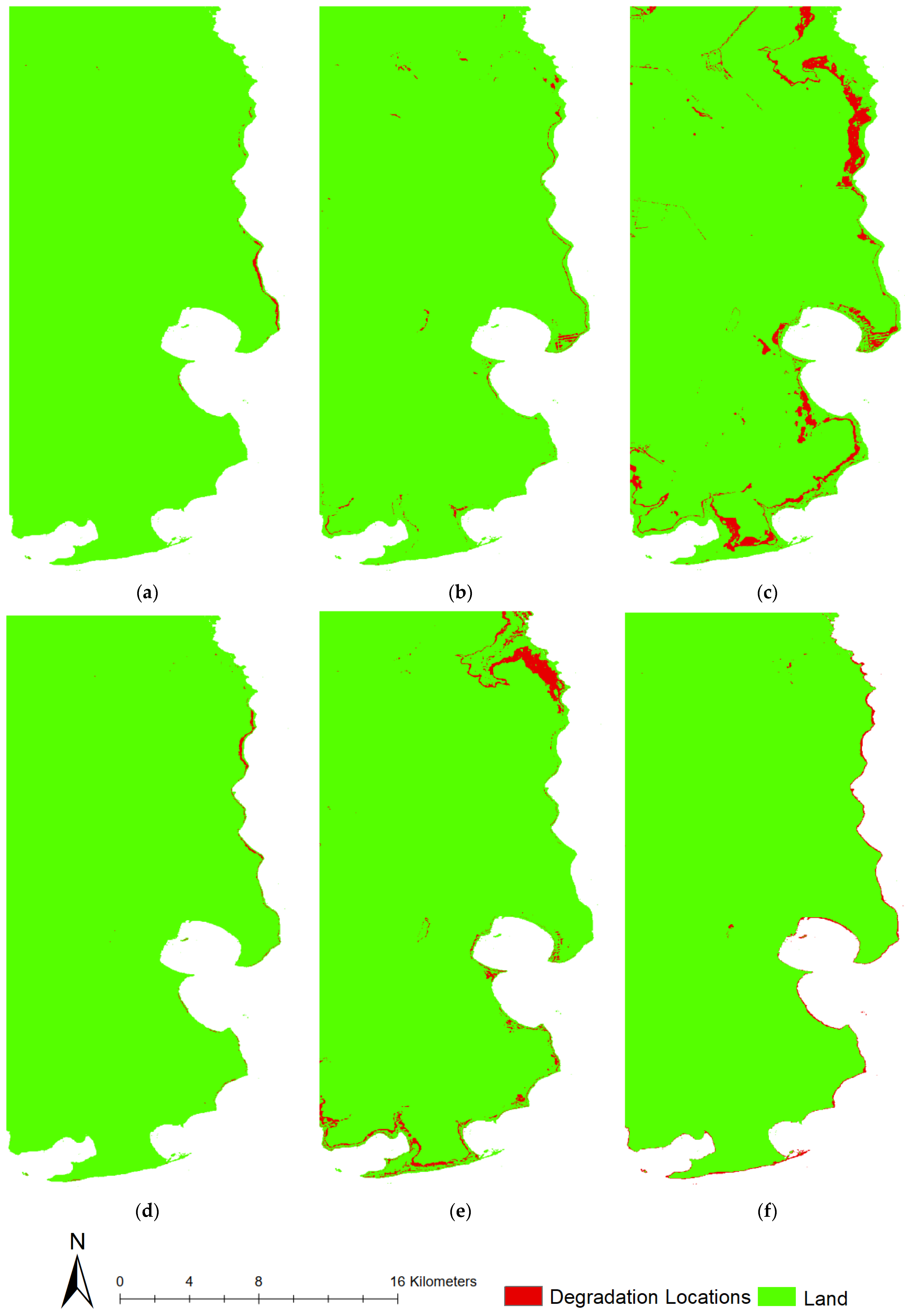
3.2.1. Detected Locations of Wetland Degradation over the ARNWR
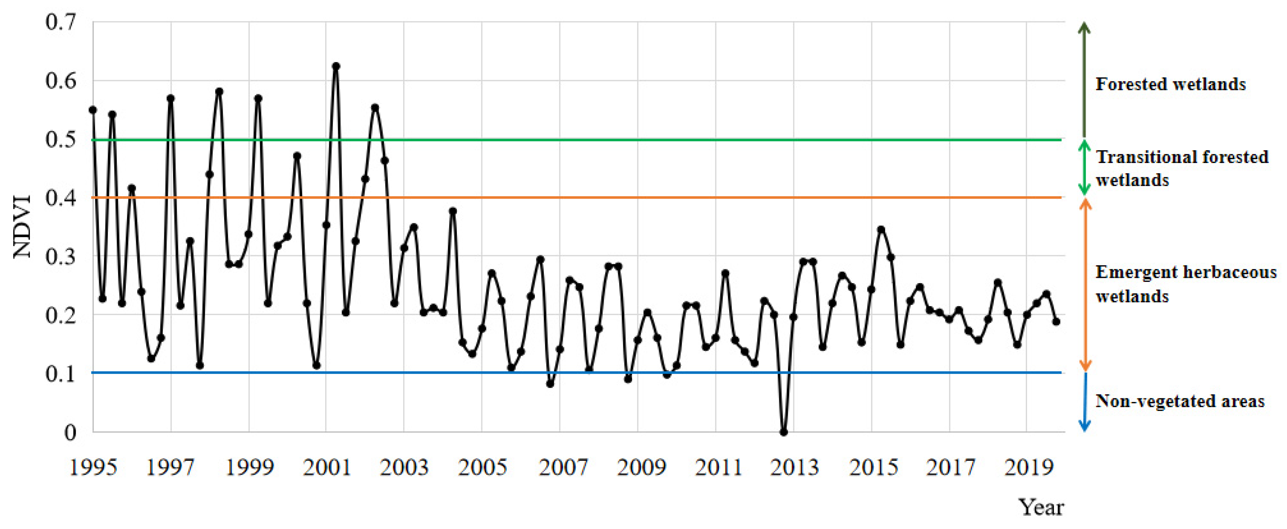
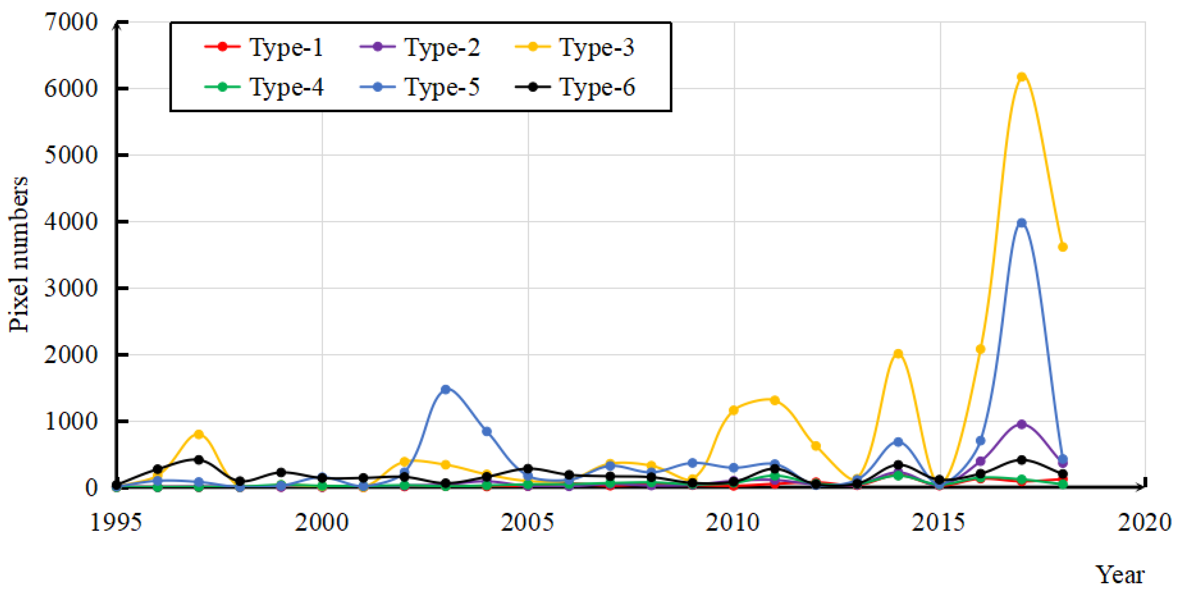
3.2.2. Detected Time of Wetland Degradation
3.2.3. Uncertainties in Detected Coastal Wetland Degradation
3.3. PIHM-Wetland Modeling Analysis
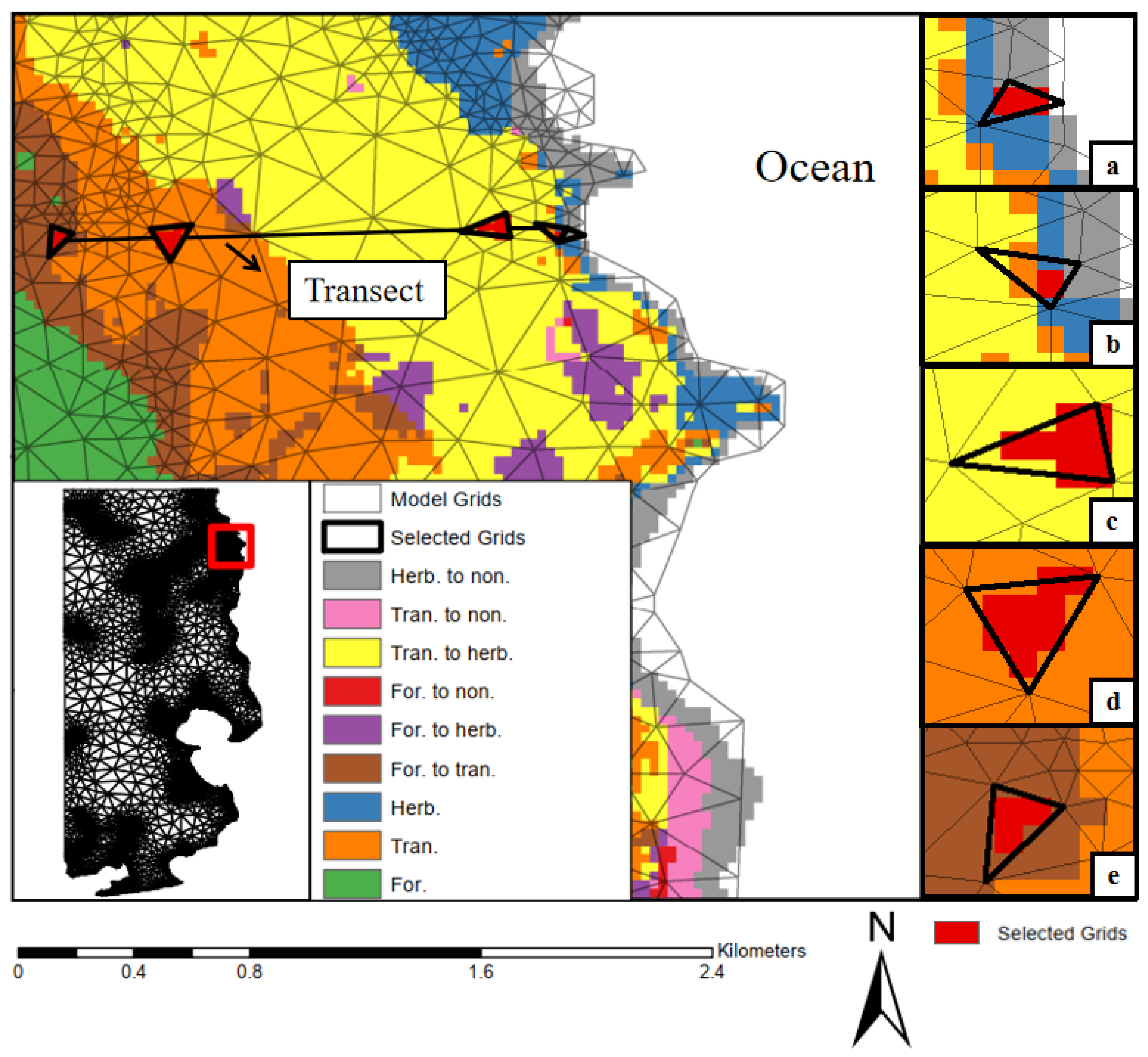
3.3.1. The Selected Transect for Analysis
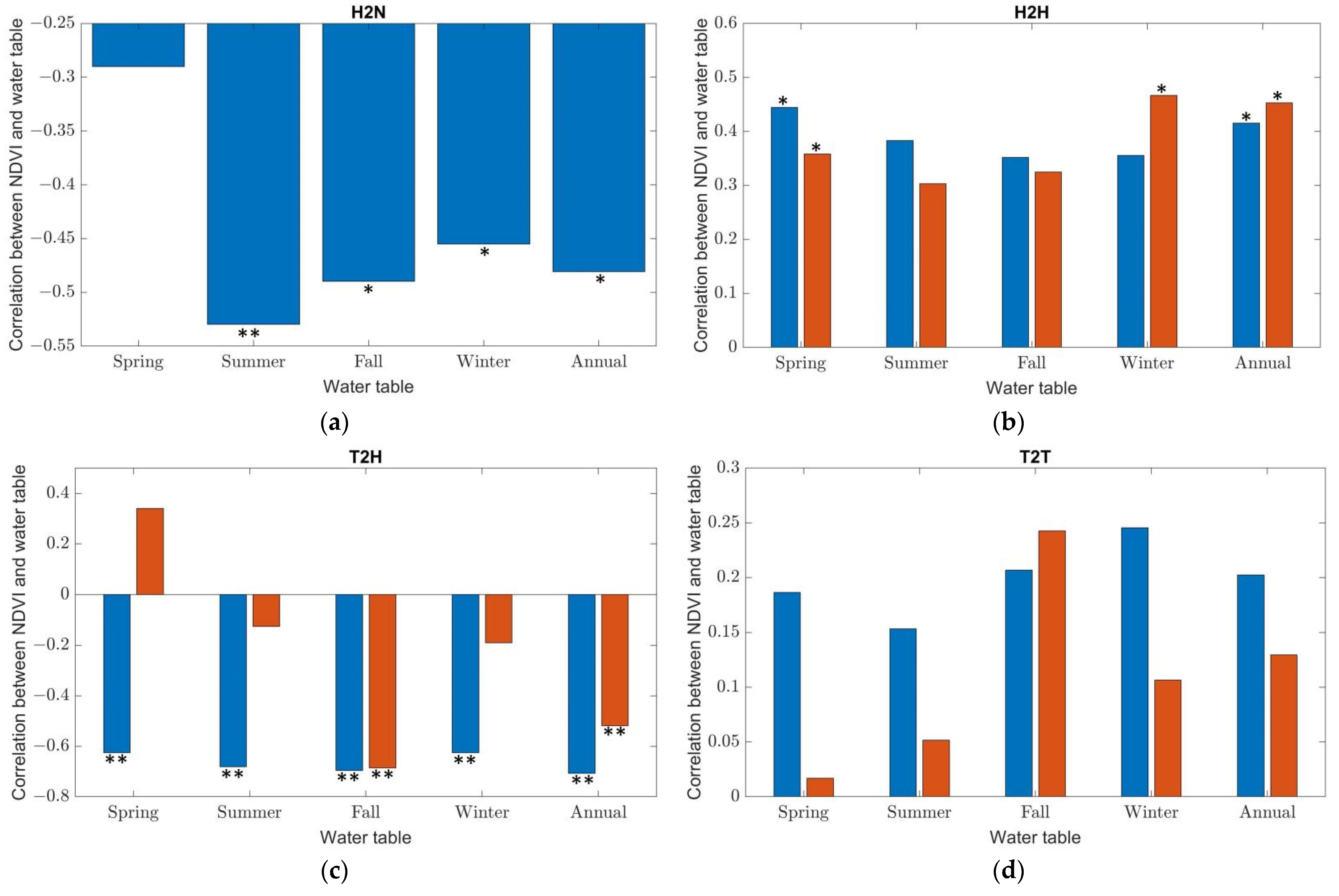
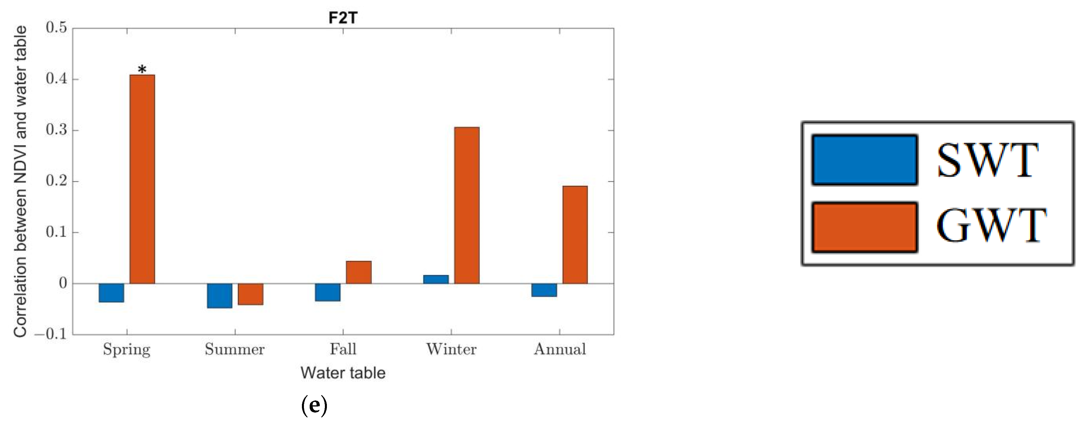
3.3.2. Correlations between NDVI and Water Tables
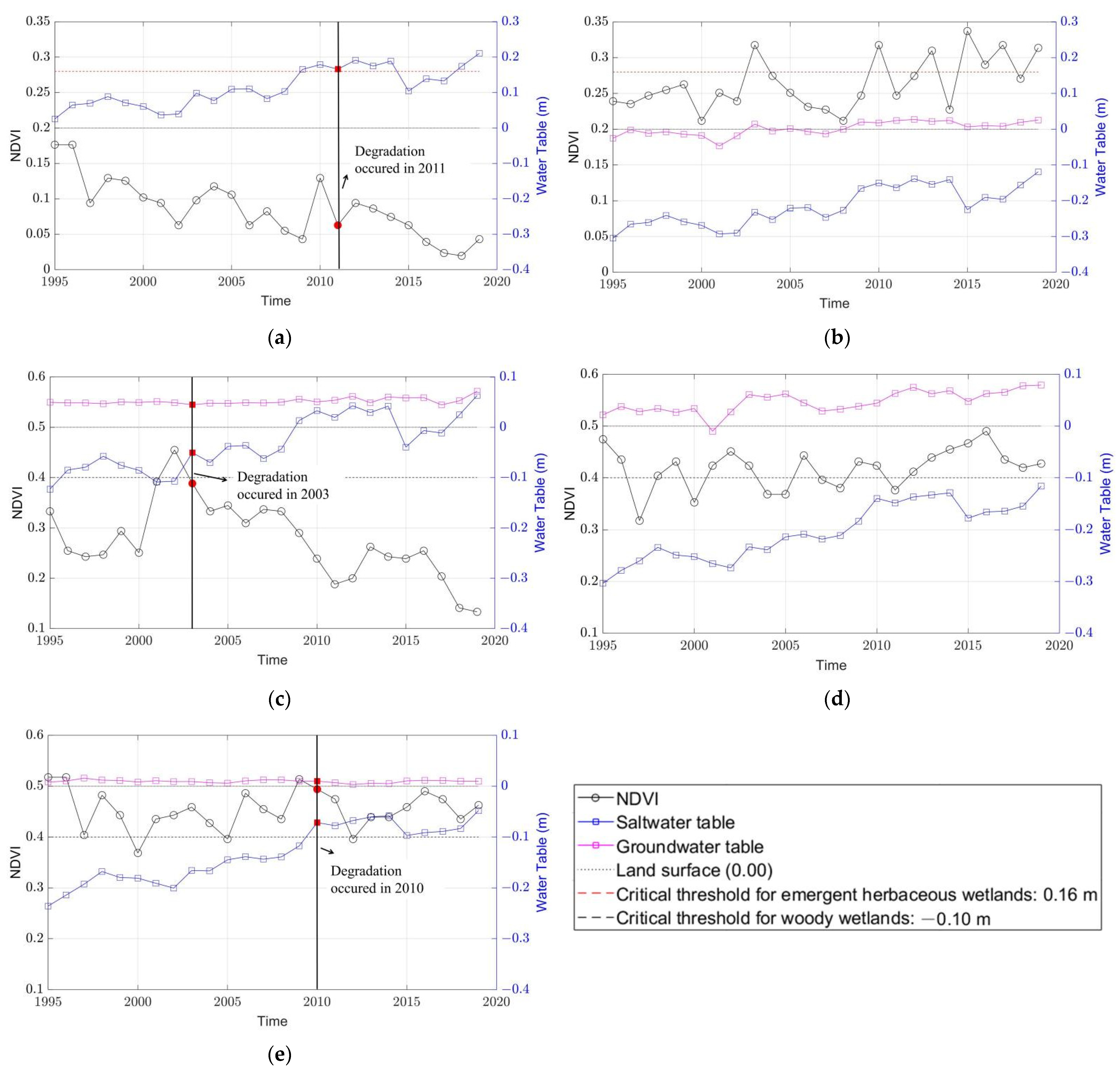
3.3.3. Thresholds of Water Table Depth to Coastal Wetland Degradation
4. Conclusions
Supplementary Materials
Author Contributions
Funding
Data Availability Statement
Acknowledgments
Conflicts of Interest
References
- Tockner, K.; Pusch, M.; Borchardt, D.; Lorang, M.S. Multiple stressors in coupled river-floodplain ecosystems. Freshw. Biol. 2010, 55, 135–151. [Google Scholar] [CrossRef]
- Amlin, N.M.; Rood, S.B. Comparative tolerances of riparian willows and cottonwoods to water-table decline. Wetlands 2002, 22, 338–346. [Google Scholar] [CrossRef]
- Conner, W.H.; Mihalia, I.; Wolfe, J. Tree community structure and changes from 1987 to 1999 in three Louisiana and three South Carolina forested wetlands. Wetlands 2002, 22, 58–70. [Google Scholar] [CrossRef]
- Day, J.W.; Christian, R.R.; Boesch, D.M.; Yáñez-Arancibia, A.; Morris, J.; Twilley, R.R.; Naylor, L.; Schaffner, L.; Stevenson, C. Consequences of Climate Change on the Ecogeomorphology of Coastal Wetlands. Estuar. Coast 2008, 31, 477–491. [Google Scholar] [CrossRef]
- Mitsch, W.J.; Gosselink, J.G. Wetlands, 5th ed.; John Wiley, Inc.: New York, NY, USA, 2015. [Google Scholar]
- Rodríguez-Iturbe, I.; Porporato, A. Ecohydrology of Water-Controlled Ecosystems: Soil Moisture and Plant Dynamics; Cambridge University Press: New York, NY, USA, 2007. [Google Scholar]
- Williams, K.; MacDonald, M.; Sternberg, L.D. Interactions of storm, drought, and sea-level rise on coastal forest: A case study. J. Coast. Res. 2003, 19, 1116–1121. [Google Scholar]
- Winter, T.C. The vulnerability of wetlands to climate change: A hydrologic landscape perspective. J. Am. Water Resour. Assoc. 2000, 36, 305–311. [Google Scholar] [CrossRef]
- Zhang, Y.; Li, W.; Sun, G.; King, J.S. Coastal wetland resilience to climate variability: A hydrologic perspective. J. Hydrol. 2019, 568, 275–284. [Google Scholar] [CrossRef]
- Zhang, Y.; Li, W.; Sun, G.; Miao, G.; Noormets, A.; Emanuel, R.; King, J.S. Understanding coastal wetland hydrology with a new regional-scale, process-based hydrological model. Hydrol. Process 2018, 32, 3158–3173. [Google Scholar] [CrossRef]
- Manzoni, S.; Maneas, G.; Scaini, A.; Psiloglou, B.E.; Destouni, G.; Lyon, S.W. Understanding coastal wetland conditions and futures by closing their hydrologic balance: The case of the Gialova lagoon, Greece. Hydrol. Earth Syst. Sci. 2020, 24, 3557–3571. [Google Scholar] [CrossRef]
- Bianchette, T.A.; Liu, K.B.; Lam, N.N.; Kiage, L.M. Ecological impacts of Hurricane Ivan on the Gulf Coast of Alabama: A remote sensing study. J. Coast. Res. 2009, SI 56, 1622–1626. [Google Scholar]
- Hopfensperger, K.N.; Burgin, A.J.; Schoepfer, V.A.; Helton, A.M. Impacts of Saltwater Incursion on Plant Communities, Anaerobic Microbial Metabolism, and Resulting Relationships in a Restored Freshwater Wetland. Ecosystems 2014, 17, 792–807. [Google Scholar] [CrossRef]
- Li, L.; Li, W.; Deng, Y. Summer rainfall variability over the Southeastern United States and its intensification in the 21st century as assessed by CMIP5 models. J. Geophys. Res. Atmos. 2013, 118, 340–354. [Google Scholar] [CrossRef]
- Li, L.; Li, W.; Fu, R.; Deng, Y.; Wang, H. Changes to the North Atlantic Subtropical High and Its Role in the Intensification of Summer Rainfall Variability in the Southeastern United States. J. Clim. 2011, 24, 1499–1506. [Google Scholar] [CrossRef] [Green Version]
- Wessels, K.J.; Van den Bergh, F.; Scholes, R.J. Limits to detectability of land degradation by trend analysis of vegetation index data. Remote Sens. Environ. 2012, 125, 10–22. [Google Scholar] [CrossRef]
- Grenfell, M.C.; Ellery, W.N.; Garden, S.E.; Dini, J.; Van der Valk, A.G. The language of intervention: A review of concepts and terminology in wetland ecosystem repair. Water SA 2007, 33, 43–50. [Google Scholar] [CrossRef] [Green Version]
- Shen, G.; Yang, X.; Jin, Y.; Xu, B.; Zhou, Q. Remote sensing and evaluation of the wetland ecological degradation process of the Zoige Plateau Wetland in China. Ecol. Indic. 2019, 104, 48–58. [Google Scholar] [CrossRef]
- Smart, L.S.; Taillie, P.J.; Poulter, B.; Vukomanovic, J.; Singh, K.K.; Swenson, J.J.; Mitasova, H.; Smith, J.W.; Meentemeyer, R.K. Aboveground carbon loss associated with the spread of ghost forests as sea levels rise. Environ. Res. Lett. 2020, 15, 104028. [Google Scholar] [CrossRef]
- Kirwan, M.L.; Gedan, K.B. Sea-level driven land conversion and the formation of ghost forests. Nat. Clim. Chang. 2019, 9, 450–457. [Google Scholar] [CrossRef] [Green Version]
- Cui, L.; Li, G.; Ouyang, N.; Mu, F.; Yan, F.; Zhang, Y.; Huang, X. Analyzing Coastal Wetland Degradation and its Key Restoration Technologies in the Coastal Area of Jiangsu, China. Wetlands 2018, 38, 525–537. [Google Scholar] [CrossRef]
- Qiu, Z.; Luo, L.; Mao, D.; Du, B.; Feng, K.; Jia, M.; Wang, Z. Using Multisource Geospatial Data to Identify Potential Wetland Rehabilitation Areas: A Pilot Study in China’s Sanjiang Plain. Water 2020, 12, 2496. [Google Scholar] [CrossRef]
- Shi, S.; Chang, Y.; Wang, G.; Li, Z.; Hu, Y.; Liu, M.; Li, Y.; Li, B.; Zong, M.; Huang, W. Planning for the wetland restoration potential based on the viability of the seed bank and the land-use change trajectory in the Sanjiang Plain of China. Sci. Total Environ. 2020, 733, 139208. [Google Scholar] [CrossRef] [PubMed]
- Huo, L.; Chen, Z.; Zou, Y.; Lu, X.; Guo, J.; Tang, X. Effect of Zoige alpine wetland degradation on the density and fractions of soil organic carbon. Ecol. Eng. 2013, 51, 287–295. [Google Scholar] [CrossRef]
- Lougheed, V.L.; McIntosh, M.D.; Parker, C.A.; Stevenson, R.J. Wetland degradation leads to homogenization of the biota at local and landscape scales. Freshw. Biol. 2008, 53, 2402–2413. [Google Scholar] [CrossRef]
- Malekmohammadi, B.; Rahimi Blouchi, L. Ecological risk assessment of wetland ecosystems using Multi Criteria Decision Making and Geographic Information System. Ecol. Indic. 2014, 41, 133–144. [Google Scholar] [CrossRef]
- Rodríguez, C.F.; Bécares, E.; Fernández-Aláez, M.; Fernández-Aláez, C. Loss of diversity and degradation of wetlands as a result of introducing exotic crayfish. Biol. Invasions 2005, 7, 75–85. [Google Scholar] [CrossRef]
- Brooks, R.P.; Wardrop, D.H.; Cole, C.A.; Campbell, D.A. Are we purveyors of wetland homogeneity?: A model of degradation and restoration to improve wetland mitigation performance. Ecol. Eng. 2005, 24, 331–340. [Google Scholar] [CrossRef]
- Keim, R.F.; Chambers, J.L.; Hughes, M.S.; Nyman, J.A.; Miller, C.A.; Amos, B.J.; Conner, W.H.; Day, J.W.; Faulkner, S.P.; Gardiner, E.S.; et al. Ecological consequences of changing hydrological conditions in wetland forests of coastal Louisiana. In Coastal Environment and Water Quality; Xu, Y.J., Singh, V.P., Eds.; 6 Water Resources Publications, LLC: Highlands Ranch, CO, USA, 2006; pp. 383–396. [Google Scholar]
- Aguilos, M.; Mitra, B.; Noormets, A.; Minick, K.; Prajapati, P.; Gavazzi, M.; Sun, G.; McNulty, S.; Li, X.; Domec, J.-C.; et al. Long-term carbon flux and balance in managed and natural coastal forested wetlands of the Southeastern USA. Agric. For. Meteorol. 2020, 288, 108022. [Google Scholar] [CrossRef]
- Uzarski, D.G.; Brady, V.J.; Cooper, M.J.; Wilcox, D.A.; Albert, D.A.; Axler, R.P.; Bostwick, P.; Brown, T.N.; Ciborowski, J.J.H.; Danz, N.P.; et al. Standardized Measures of Coastal Wetland Condition: Implementation at a Laurentian Great Lakes Basin-Wide Scale. Wetlands 2017, 37, 15–32. [Google Scholar] [CrossRef]
- Doyle, C.; Beach, T.; Luzzadder-Beach, S. Tropical Forest and Wetland Losses and the Role of Protected Areas in Northwestern Belize, Revealed from Landsat and Machine Learning. Remote Sens. 2021, 13, 379. [Google Scholar] [CrossRef]
- Ury, E.A.; Yang, X.; Wright, J.P.; Bernhardt, E.S. Rapid deforestation of a coastal landscape driven by sea-level rise and extreme events. Ecol. Appl. 2021, 31, e02339. [Google Scholar] [CrossRef]
- Guo, M.; Li, J.; Sheng, C.; Xu, J.; Wu, L. A Review of Wetland Remote Sensing. Sensors 2017, 17, 777. [Google Scholar] [CrossRef] [PubMed] [Green Version]
- Jin, H.; Huang, C.; Lang, M.W.; Yeo, I.-Y.; Stehman, S.V. Monitoring of wetland inundation dynamics in the Delmarva Peninsula using Landsat time-series imagery from 1985 to 2011. Remote Sens. Environ. 2017, 190, 26–41. [Google Scholar] [CrossRef] [Green Version]
- Klemas, V. Remote sensing techniques for studying coastal ecosystems: An overview. J. Coast. Res. 2011, 27, 2–17. [Google Scholar]
- Jiang, Z.; Huete, A.R.; Chen, J.; Chen, Y.; Li, J.; Yan, G.; Zhang, X. Analysis of NDVI and scaled difference vegetation index retrievals of vegetation fraction. Remote Sens. Environ. 2006, 101, 366–378. [Google Scholar] [CrossRef]
- Lambert, J.; Denux, J.-P.; Verbesselt, J.; Balent, G.; Cheret, V. Detecting Clear-Cuts and Decreases in Forest Vitality Using MODIS NDVI Time Series. Remote Sens. 2015, 7, 3588–3612. [Google Scholar] [CrossRef] [Green Version]
- Klemas, V. Remote sensing of emergent and submerged wetlands: An overview. Int. J. Remote Sens. 2013, 34, 6286–6320. [Google Scholar] [CrossRef]
- Yuan, J.; Cohen, M.J. Remote detection of ecosystem degradation in the Everglades ridge-slough landscape. Remote Sens. Environ. 2020, 247, 111917. [Google Scholar] [CrossRef]
- Bai, Z.G.; Dent, D.L.; Olsson, L.; Schaepman, M.E. Proxy global assessment of land degradation. Soil Use Manag. 2008, 24, 223–234. [Google Scholar] [CrossRef]
- Colwell, J.E. Vegetation canopy reflectance. Remote Sens. Environ. 1974, 3, 175–183. [Google Scholar] [CrossRef]
- Huete, A.R.; Liu, H.Q.; Batchily, K.V.; Van Leeuwen, W.J. A comparison of vegetation indices over a global set of TM images for EOS-MODIS. Remote Sens. Environ. 1997, 59, 440–451. [Google Scholar] [CrossRef]
- Pereira, O.; Ferreira, L.; Pinto, F.; Baumgarten, L. Assessing Pasture Degradation in the Brazilian Cerrado Based on the Analysis of MODIS NDVI Time-Series. Remote Sens. 2018, 10, 1761. [Google Scholar] [CrossRef] [Green Version]
- Eckert, S.; Hüsler, F.; Liniger, H.; Hodel, E. Trend analysis of MODIS NDVI time series for detecting land degradation and regeneration in Mongolia. J. Arid Environ. 2015, 113, 16–28. [Google Scholar] [CrossRef]
- Moorhead, K.K.; Brinson, M.M. Response of wetlands to rising sea level in the lower coastal plain of North Carolina. Ecol. Appl. 1995, 5, 261–271. [Google Scholar] [CrossRef]
- Moorhead, K.K.; Cook, A.E. A comparison of hydric soils, wetlands, and land use in coastal North Carolina. Wetlands 1992, 12, 99–105. [Google Scholar] [CrossRef]
- Poulter, B. Interactions between Landscape Disturbance and Gradual Environmental Change: Plant Community Migration in Response to Fire and Sea Level Rise. Ph.D. Thesis, Duke University, Durham, NC, USA, 2005. [Google Scholar]
- Taillie, P.J.; Moorman, C.E.; Poulter, B.; Ardón, M.; Emanuel, R.E. Decadal-Scale Vegetation Change Driven by Salinity at Leading Edge of Rising Sea Level. Ecosystems 2019, 22, 1918–1930. [Google Scholar] [CrossRef]
- Aguilos, M.; Sun, G.; Noormets, A.; Domec, J.C.; Mcnulty, S.; Gavazzi, M.; Prajapati, P.; Minick, K.J.; Mitra, B.; King, J. Ecosystem productivity and evapotranspiration are tightly coupled in Loblolly Pine (Pinus taeda L.) plantations along the coastal plain of the southeastern US. Forests 2021, 12, 1123. [Google Scholar] [CrossRef]
- Miao, G.; Noormets, A.; Domec, J.C.; Trettin, C.C.; McNulty, S.G.; Sun, G.; King, J.S. The effect of water table fluctuation on soil respiration in a lower coastal plain forested wetland in the southeastern US. J. Geophys. Res.-Biogeosci. 2013, 118, 1748–1762. [Google Scholar] [CrossRef]
- Schieder, N.W.; Walters, D.C.; Kirwan, M.L. Massive Upland to Wetland Conversion Compensated for Historical Marsh Loss in Chesapeake Bay, USA. Estuar. Coast 2018, 41, 940–951. [Google Scholar] [CrossRef]
- Walker, J.S.; Kopp, R.E.; Shaw, T.A.; Cahill, N.; Khan, N.S.; Barber, D.C.; Ashe, E.L.; Brain, M.J.; Clear, J.L.; Corbett, D.R.; et al. Common Era sea-level budgets along the U.S. Atlantic coast. Nat. Commun. 2021, 12, 1841. [Google Scholar] [CrossRef]
- Hunter, R.G.; Day, J.W.; Lane, R.R.; Shaffer, G.P.; Day, J.N.; Conner, W.H.; Rybczyk, J.M.; Mistich, J.A.; Ko, J.Y. Using natural wetlands for municipal effluent assimilation: A half-century of experience for the Mississippi River Delta and surrounding environs. In Multifunctional Wetlands; Nagabhatla, N., Metcalfe, C.D., Eds.; Springer Nature: Cham, Switzerland, 2018; pp. 15–81. [Google Scholar]
- Lang, M.; Stedman, S.-M.; Nettles, J.; Griffin, R. Coastal Watershed Forested Wetland Change and Opportunities for Enhanced Collaboration with the Forestry Community. Wetlands 2020, 40, 7–19. [Google Scholar] [CrossRef]
- Richardson, C.J. Pocosins: An ecological perspective. Wetlands 1991, 11, 335–354. [Google Scholar] [CrossRef]
- Kennedy, R.E.; Andréfouët, S.; Cohen, W.B.; Gómez, C.; Griffiths, P.; Hais, M.; Healey, S.P.; Helmer, E.H.; Hostert, P.; Lyons, M.B.; et al. Bringing an ecological view of change to Landsat-based remote sensing. Front. Ecol. Environ. 2014, 12, 339–346. [Google Scholar] [CrossRef]
- Wulder, M.A.; Masek, J.G.; Cohen, W.B.; Loveland, T.R.; Woodcock, C.E. Opening the archive: How free data has enabled the science and monitoring promise of Landsat. Remote Sens. Environ. 2012, 122, 2–10. [Google Scholar] [CrossRef]
- Eidenshink, J. The 1990 conterminous U. S. AVHRR data set. Photogramm. Eng. Remote Sens. 1992, 58, 809–813. [Google Scholar]
- Gamon, J.A.; Field, C.B.; Goulden, M.L.; Griffin, K.L.; Hartley, A.E.; Joel, G.; Penuelas, J.; Valentini, R. Relationships between NDVI, canopy structure, and photosynthesis in three Californian vegetation types. Ecol. Appl. 1995, 5, 28–41. [Google Scholar] [CrossRef] [Green Version]
- Sun, C.; Liu, Y.; Zhao, S.; Zhou, M.; Yang, Y.; Li, F. Classification mapping and species identification of salt marshes based on a short-time interval NDVI time-series from HJ-1 optical imagery. Int. J. Appl. Earth Obs. 2016, 45, 27–41. [Google Scholar] [CrossRef]
- Zhang, X.; Wu, S.; Yan, X.; Chen, Z. A global classification of vegetation based on NDVI, rainfall and temperature. Int. J. Climatol. 2017, 37, 2318–2324. [Google Scholar] [CrossRef]
- Jamali, S.; Seaquist, J.; Eklundh, L.; Ardö, J. Automated mapping of vegetation trends with polynomials using NDVI imagery over the Sahel. Remote Sens. Environ. 2014, 141, 79–89. [Google Scholar] [CrossRef]
- Karlsen, S.; Elvebakk, A.; Høgda, K.; Grydeland, T. Spatial and Temporal Variability in the Onset of the Growing Season on Svalbard, Arctic Norway—Measured by MODIS-NDVI Satellite Data. Remote Sens. 2014, 6, 8088–8106. [Google Scholar] [CrossRef] [Green Version]
- Anyamba, A.; Tucker, C.J. Analysis of Sahelian vegetation dynamics using NOAA-AVHRR NDVI data from 1981–2003. J. Arid Environ. 2005, 63, 596–614. [Google Scholar] [CrossRef]
- Zheng, Y.; Han, J.; Huang, Y.; Fassnacht, S.R.; Xie, S.; Lv, E.; Chen, M. Vegetation response to climate conditions based on NDVI simulations using stepwise cluster analysis for the Three-River Headwaters region of China. Ecol. Indic. 2018, 92, 18–29. [Google Scholar] [CrossRef]
- Bhandari, A.K.; Kumar, A.; Singh, G.K. Feature Extraction using Normalized Difference Vegetation Index (NDVI): A Case Study of Jabalpur City. Proc. Technol. 2012, 6, 612–621. [Google Scholar] [CrossRef] [Green Version]
- Chouhan, A.P.S.; Sarma, A.K. Modern heterogeneous catalysts for biodiesel production: A comprehensive review. Renew. Sustain. Energy Rev. 2011, 15, 4378–4399. [Google Scholar] [CrossRef]
- Gandhi, G.M.; Parthiban, S.; Thummalu, N.; Christy, A. Ndvi: Vegetation Change Detection Using Remote Sensing and Gis—A Case Study of Vellore District. Procedia Comput. Sci. 2015, 57, 1199–1210. [Google Scholar] [CrossRef] [Green Version]
- Meneses-Tovar, C.L. NDVI as indicator of degradation. Unasylva 2011, 62, 39–46. [Google Scholar]
- Rousta, I.; Olafsson, H.; Moniruzzaman, M.; Ardö, J.; Zhang, H.; Mushore, T.D.; Shahin, S.; Azim, S. The 2000–2017 drought risk assessment of the western and southwestern basins in Iran. Model. Earth Syst. Environ. 2020, 6, 1201–1221. [Google Scholar] [CrossRef]
- Weier, J.; Herring, D. Measuring Vegetation (NDVI & EVI); NASA Earth Observatory: Washington, DC, USA, 2000.
- Bechtold, W.A.; Patterson, P.L. (Eds.) The Enhanced Forest Inventory and Analysis Program-National Sampling Design and Estimation Procedures. Gen. Technol. Rep. SRS-80; U.S. Department of Agriculture, Forest Service, Southern Research Station: Asheville, NC, USA, 2005; p. 85.
- Burrill, E.A.; DiTommaso, A.M.; Turner, J.A.; Pugh, S.A.; Menlove, J.; Christiansen, G.; Perry, C.J.; Conkling, B.L. The Forest Inventory and Analysis Database: Database Description and User Guide Version 9.0.1 for Phase 2. U.S. Department of Agriculture, Forest Service. 1026p. Available online: http://www.fia.fs.fed.us/library/database-documentation/ (accessed on 21 September 2020).
- C-CAP Regional Land Cover and Change. NOAA. Available online: www.coast.noaa.gov/htdata/raster1/landcover/bulkdownload/30m_lc/ (accessed on 20 July 2021).
- Xia, Y.; Mitchell, K.; Ek, M.; Sheffield, J.; Cosgrove, B.; Wood, E.; Luo, L.; Alonge, C.; Wei, H.; Meng, J.; et al. Continental-scale water and energy flux analysis and validation for the North American Land Data Assimilation System project phase 2 (NLDAS-2): 1. Intercomparison and application of model products. J. Geophys. Res. Atmos. 2012, 117, D03109. [Google Scholar] [CrossRef]
- Nash, J.E.; Sutcliffe, J.V. River flow forecasting through conceptual models part I—A discussion of principles. J. Hydrol. 1970, 10, 282–290. [Google Scholar] [CrossRef]
- Liu, Y.; Kumar, M. Role of meteorological controls on interannual variations in wet-period characteristics of wetlands. Water Resour. Res. 2016, 52, 5056–5074. [Google Scholar] [CrossRef] [Green Version]
- Todd, M.J.; Muneepeerakul, R.; Pumo, D.; Azaele, S.; Miralles-Wilhelm, F.; Rinaldo, A.; Rodriguez-Iturbe, I. Hydrological drivers of wetland vegetation community distribution within Everglades National Park, Florida. Adv. Water Resour. 2010, 33, 1279–1289. [Google Scholar] [CrossRef]
- Wei, J.; Huang, W.; Li, Z.; Sun, L.; Zhu, X.; Yuan, Q.; Liu, L.; Cribb, M. Cloud detection for Landsat imagery by combining the random forest and superpixels extracted via energy-driven sampling segmentation approaches. Remote Sens. Environ. 2020, 248, 112005. [Google Scholar] [CrossRef]
- Zhu, Z.; Qiu, S.; He, B.; Deng, C. Cloud and cloud shadow detection for Landsat images: The fundamental basis for analyzing Landsat time series. In Remote Sensing Time Series Image Processing; Weng, Q., Ed.; CRC Press: Boca Raton, FL, USA, 2018; pp. 3–23. [Google Scholar]
- Armitage, A.R.; Weaver, C.A.; Kominoski, J.S.; Pennings, S.C. Resistance to Hurricane Effects Varies Among Wetland Vegetation Types in the Marsh–Mangrove Ecotone. Estuar. Coast 2020, 43, 960–970. [Google Scholar] [CrossRef]
- Hu, T.; Smith, R. The Impact of Hurricane Maria on the Vegetation of Dominica and Puerto Rico Using Multispectral Remote Sensing. Remote Sens. 2018, 10, 827. [Google Scholar] [CrossRef] [Green Version]
- Steyer, G.D.; Couvillion, B.R.; Barras, J.A. Monitoring Vegetation Response to Episodic Disturbance Events by using Multitemporal Vegetation Indices. J. Coast. Res. 2013, 63, 118–130. [Google Scholar] [CrossRef]
- Ke, Y.; Im, J.; Lee, J.; Gong, H.; Ryu, Y. Characteristics of Landsat 8 OLI-derived NDVI by comparison with multiple satellite sensors and in-situ observations. Remote Sens. Environ. 2015, 164, 298–313. [Google Scholar] [CrossRef]
- Roy, D.P.; Kovalskyy, V.; Zhang, H.K.; Vermote, E.F.; Yan, L.; Kumar, S.S.; Egorov, A. Characterization of Landsat-7 to Landsat-8 reflective wavelength and normalized difference vegetation index continuity. Remote Sens. Environ. 2016, 185, 57–70. [Google Scholar] [CrossRef] [Green Version]
- Xu, D.; Guo, X. Compare NDVI Extracted from Landsat 8 Imagery with that from Landsat 7 Imagery. Am. J. Remote Sens. 2014, 2, 10–14. [Google Scholar] [CrossRef] [Green Version]
- Cairns, J., Jr. Setting ecological restoration goals for technical feasibility and scientific validity. Ecol. Eng. 2000, 15, 171–180. [Google Scholar] [CrossRef]
- Kentula, M.E. Perspectives on setting success criteria for wetland restoration. Ecol. Eng. 2000, 15, 199–209. [Google Scholar] [CrossRef]
- Broadfoot, W.M.; Williston, H.L. Flooding effects on southern forests. J. For. 1973, 71, 584–587. [Google Scholar]
- Copini, P.; Den Ouden, J.; Robert, E.M.; Tardif, J.C.; Loesberg, W.A.; Goudzwaard, L.; Sass-Klaassen, U. Flood-ring formation and root development in response to experimental flooding of young Quercus robur trees. Front. Plant Sci. 2016, 7, 775. [Google Scholar] [CrossRef] [PubMed] [Green Version]
- Siebel, H.N.; Blom, C.W. Effects of irregular flooding on the establishment of tree species. Acta Bot. Neerl. 1998, 47, 231–240. [Google Scholar]
- Xu, H.; Ye, M.; Li, J.-M. Changes in groundwater levels and the response of natural vegetation to transfer of water to the lower reaches of the Tarim River. J. Environ. Sci. 2007, 19, 1199–1207. [Google Scholar] [CrossRef]
- Kirwan, M.L.; Kirwan, J.L.; Copenheaver, C.A. Dynamics of an Estuarine Forest and its Response to Rising Sea Level. J. Coast. Res. 2007, 232, 457–463. [Google Scholar] [CrossRef]
- Costa, C.S.; Marangoni, J.C.; Azevedo, A.M. Plant zonation in irregularly flooded salt marshes: Relative importance of stress tolerance and biological interactions. J. Ecol. 2003, 91, 951–965. [Google Scholar] [CrossRef]
- Kemp, A.C.; Horton, B.P.; Culver, S.J. Distribution of modern salt-marsh foraminifera in the Albemarle–Pamlico estuarine system of North Carolina, USA: Implications for sea-level research. Mar. Micropaleontol. 2009, 72, 222–238. [Google Scholar] [CrossRef]
- Poulter, B.; Christensen, N.L.; Qian, S.S. Tolerance of Pinus taeda and Pinus serotina to low salinity and flooding: Implications for equilibrium vegetation dynamics. J. Veg. Sci. 2008, 19, 15–22. [Google Scholar] [CrossRef]


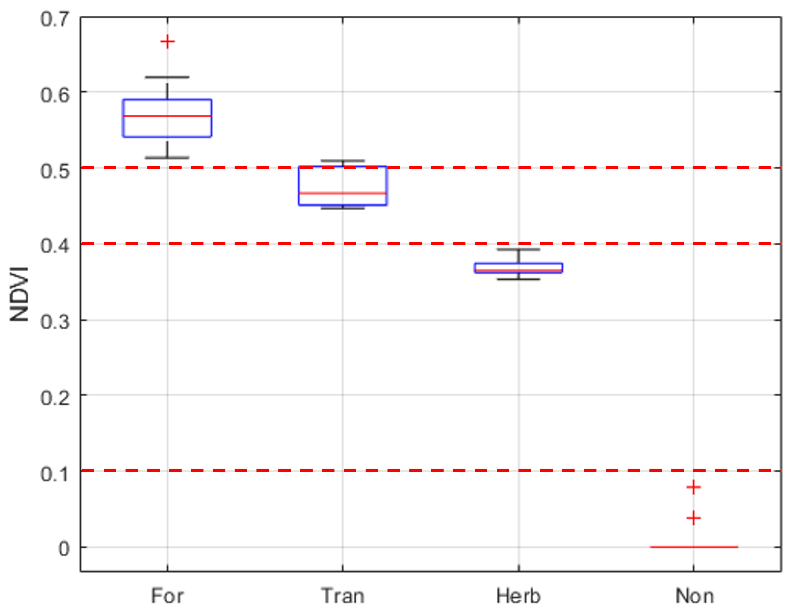
| Coastal Wetland Types | NDVI Ranges | Structural Complexity |
|---|---|---|
| Forested wetlands | 0.5 ≤ NDVI ≤ 1.0 | Very High |
| Transitional forested wetlands | 0.4 ≤ NDVI < 0.5 | High |
| Emergent herbaceous wetlands | 0.1 ≤ NDVI < 0.4 | Moderate |
| Non-vegetated areas | −1.0 ≤ NDVI < 0.1 | Low |
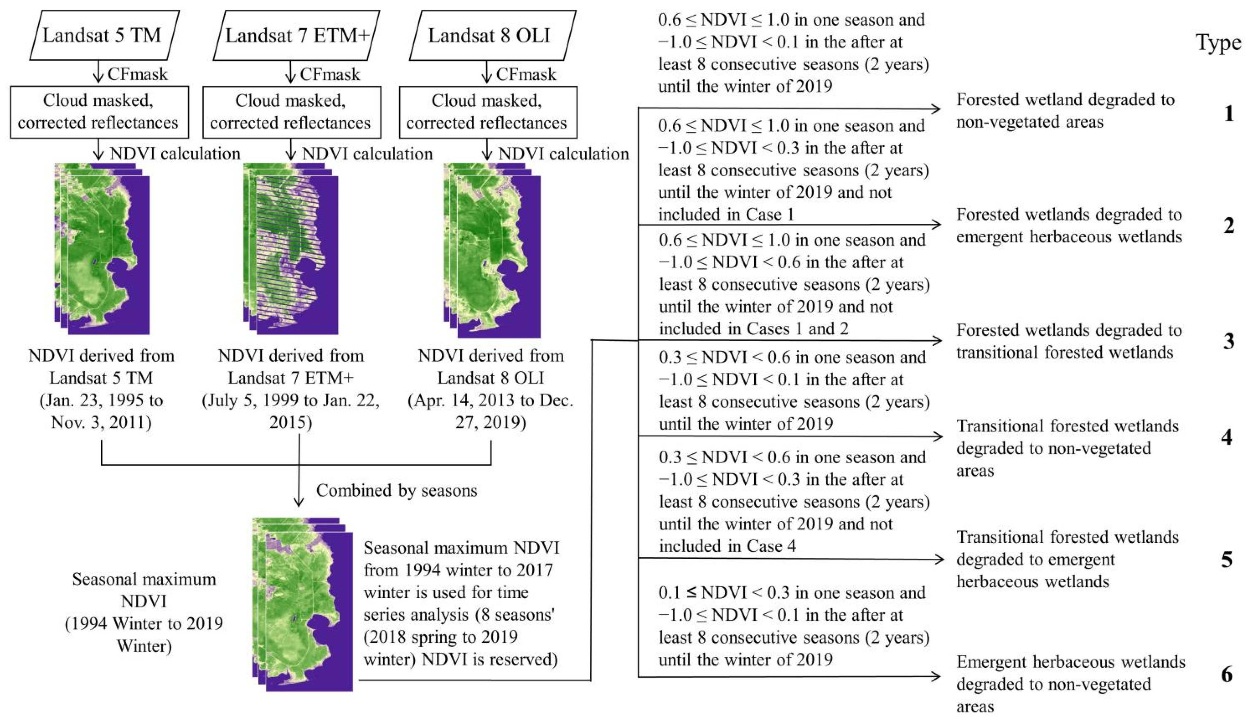
| Type | Wetland Degradation Types | Number of Wetland Degradation Pixels 1 | Areas of Wetland Degradation (Hectares) | Degradation Percentage of the Study Area (%) |
|---|---|---|---|---|
| 1 | Forested wetland degraded to non-vegetated areas | 930 | 84 | 0.21 |
| 2 | Forested wetlands degraded to emergent herbaceous wetlands | 2538 | 228 | 0.56 |
| 3 | Forested wetlands degraded to transitional forested wetlands | 20,011 | 1801 | 4.44 |
| 4 | Transitional forested wetlands degraded to non-vegetated areas | 1276 | 115 | 0.28 |
| 5 | Transitional forested wetlands degraded to emergent herbaceous wetlands | 10,681 | 961 | 2.37 |
| 6 | Emergent herbaceous wetlands degraded to non-vegetated areas | 4224 | 380 | 0.94 |
| Sum | 39,660 | 3569 | 8.80 | |
Publisher’s Note: MDPI stays neutral with regard to jurisdictional claims in published maps and institutional affiliations. |
© 2022 by the authors. Licensee MDPI, Basel, Switzerland. This article is an open access article distributed under the terms and conditions of the Creative Commons Attribution (CC BY) license (https://creativecommons.org/licenses/by/4.0/).
Share and Cite
He, K.; Zhang, Y.; Li, W.; Sun, G.; McNulty, S. Detecting Coastal Wetland Degradation by Combining Remote Sensing and Hydrologic Modeling. Forests 2022, 13, 411. https://doi.org/10.3390/f13030411
He K, Zhang Y, Li W, Sun G, McNulty S. Detecting Coastal Wetland Degradation by Combining Remote Sensing and Hydrologic Modeling. Forests. 2022; 13(3):411. https://doi.org/10.3390/f13030411
Chicago/Turabian StyleHe, Keqi, Yu Zhang, Wenhong Li, Ge Sun, and Steve McNulty. 2022. "Detecting Coastal Wetland Degradation by Combining Remote Sensing and Hydrologic Modeling" Forests 13, no. 3: 411. https://doi.org/10.3390/f13030411