Article

Economic and Ecological Impacts of Adjusting the Age-Class Structure in Korean Forests: Application of Constraint on the Period-to-Period Variation in Timber Production for Long-Term Forest Management

1
Department of Agriculture, Forestry and Bioresources, Seoul National University, Seoul 08826, Republic of Korea
2
Division of International Cooperation, Korea Forest Service, Daejeon 35208, Republic of Korea
3
Research Institute for Agriculture and Life Sciences, Seoul National University, Seoul 08826, Republic of Korea
4
Division of Forest Policy and Economics, National Institute of Forest Science, Seoul 02445, Republic of Korea
*
Author to whom correspondence should be addressed.
Forests 2022, 13(12), 2144; https://doi.org/10.3390/f13122144
Submission received: 3 November 2022 / Revised: 8 December 2022 / Accepted: 13 December 2022 / Published: 14 December 2022
(This article belongs to the Special Issue Climate Change and Timber Market)

Abstract

:
South Korea’s successful reforestation efforts over the past 50 years have led to abundant forest resources. However, intensive reforestation during the 1970s and 1980s skewed the forests’ age distribution towards forest stands aged 30 years or older, which results in an unbalanced distribution of age-class, requiring redistribution with harvest and effective regeneration plans to produce a sustained yield of timber as well as long term ecological benefits. During this conversion process, variations in timber production can occur, causing economic and ecological risks if excessive. To prevent these likely risks, permissible levels of increase and decrease in timber production can be restricted in the planning phase. In determining the appropriate variation rate in timber production, it is necessary to understand the impacts of variation in timber production on forest management. This study performed a sensitivity analysis to evaluate the economic and ecological impacts of constraining the period-to-period variation in timber production. A multi-objective linear programming (MOLP) forest management planning model was utilized to study forests in Mt. Gari, South Korea. Nine management alternatives were set with different levels of variation rate in timber production and further constraints. The total volume and net present value (NPV) of timber production, carbon storage, and water storage were analyzed for each alternative. As timber production variation rates decreased, the amount of timber production increased and forest carbon storage decreased; furthermore, NPV diminished as variation constraints strengthened. These differences were mainly caused by selection of regeneration species according to the constraint on variation in timber production. If the variation rate was strictly restricted, the area of timber species with short rotation age increased during conversion period, in order to reduce the gap of timber production between periods. At the latter part of planning horizon, the area of broad-leaved trees was enlarged as the burden of adjusting age-class structure reduced. The appropriate variation rate in timber production was determined to be 30%, based on considerations regarding the economic and ecological impact of the variation on the forest.

1. Introduction

In South Korea, forests account for 63% of land cover, with an average growing stock of 161.5 m3 per hectare as of 2019 [1]. The abundant Korean forestry today resulted from an intensive national reforestation project in South Korea during the 1970s and 1980s. After grand-scale reforestation, South Korea’s forest management policy concentrated on protecting and nurturing forests [2]. As a result, forests’ growing stock and public value increased significantly (Figure 1). However, since then, there has been little circulation of forest resources through continuous harvest and regeneration. Consequently, there is an unbalanced forest stand age class distribution, where stands over 31 years account for 72% of the total forest area, as shown in Figure 2.
If the current age-class imbalance persists, it would be challenging to produce a sustained timber yield in the long term. In addition, ecological forest functions, such as carbon absorption, water flow, and biodiversity, which change with forest aging [2], may be affected. Böttcher et al. [4] asserted that the forest age-class structure of a country determines how much carbon can be absorbed in present and future conditions. They demonstrated that the current age class distribution affects carbon levels and projected future carbon changes.
A country with predominantly young forests (i.e., a left-shift age-class structure) will see increasing forest carbon stocks, whereas a country with predominantly older forests (i.e., a right-shift age-class structure) is likely to see decreasing carbon stocks with the same management regime [4]. The Korea Forest Service has recognized the structural vulnerability of forests and emphasized the necessity of improving age-class distribution [5]. However, few studies have been conducted to investigate the impacts of an imbalanced forest age-class structure and how industrial forestry would vary regarding supply sustainability to redress this issue.
It is vital to develop a long-term forest management plan, including decisions regarding quantity and timing of timber harvests, and forest regeneration to transform the age-class structure of forests. Linear programming (LP) has been used to establish harvest and regeneration plans in forestry since the 1960s [6,7,8,9,10,11,12,13,14,15,16,17,18]. Some extensions of LP, such as goal programming (GP), multi-objective linear programming (MOLP), and integer programming (IP), have also been widely applied in forest management planning to calculate the harvest amount required to create sustainable forest age-class composition.
Won et al. [5] studied the composition of age-class structure over the long term in Korean forests. They used GP to estimate the optimal timber harvest volumes, facilitating evenly distributed forest age classes and harvest volumes for 50 years. Roise et al. [19], Chung and Park [20], Park and Chung [21], and Kim et al. [22] applied the MOLP to establish forest management plans that met the objectives of forest ecosystems, concerning elements such as wildlife habitat, carbon absorption, and water storage, with consideration of temporal changes in forest age class distribution. Won et al. [23] deduced optimal harvest volume maximization for individual stands considering tree species, applicable practices, and age-class distribution using IP. Costa et al. [24] also applied IP to obtain a management plan that maximizes the volume of timber harvested while also enabling a balanced age class structure at the end of the planning period. Cabral et al. [25], in another study, applied IP to formulate a forest management plan to a large forest area considering the number of owners or management bodies. Their resulting planning model returns the harvest schedule that maximizes the volume of timber harvested while ensuring sustainability, environmental constraints, and revenues of different management bodies.
Aggregately, these linear programming planning models often involve constraints related to long-term sustained yield (LTSY) for sustainable forest management. LTSY is the harvest from a regulated forest, and achieving LTSY can be interpreted as attaining a balanced age-class distribution [26]. Theoretically, LTSY means that the amount of growth matches the yield; therefore, timber production is the same yearly [27]. However, considering the actual forest management conditions, it is difficult to match the timber production for every period accurately. Instead, it is possible to improve the stability of forest management over time by adding a constraint limiting timber production level variability.
When constraining timber production variation rates, setting an appropriate level of variation is vital. For example, if excessive amounts of forest trees are cut at one time compared to the preceding period, ecological risks would occur, and the amounts harvested after that period will be reduced. However, economic losses may occur if harvest amounts are much less than in the previous period. Therefore, when formulating harvest and regeneration plans, the permissible timber production levels should be set appropriately based on understanding the economic and ecological impacts of variations in timber production.
However, previous studies have assigned arbitrary values as the input in the constraint on timber production variation without any analysis of the impacts of variation on forests. For example, the LP model developed by Chung and Park [20] included a constraint on the allowable decrease in timber production by period, which arbitrarily applied a 5% or 10% constraint. Won et al. [5] included a 10% target maximum period-to-period timber production variation as one of the four management goals of an optimal harvest plan. Nevertheless, there was no concrete evidence of why 10% was selected as the value. The MOLP model of Park and Chung [21] also constrained the upper and lower bounds of timber production for LTSY, but 10% was applied congruently to all alternatives as a constraint. The optimization results of the planning models differed depending on the period-to-period variation rate in timber production.
This study aimed at quantitatively analyzing the economic and ecological impacts caused by constraints on the period-to-period variation in timber production and providing information that can be used to determine the appropriate variation rate in timber production when establishing a long-term plan (150 years) for improving the age-class distribution of forests in South Korea. The economic and ecological impacts were analyzed by comparing alternatives with different constraints on the variation in timber production using the MOLP-based forest management model. In addition, this study investigated the appropriate variation rate in timber production, which comprehensively considers economic and ecological impacts of the variation on the forest.

2. Materials and Methods
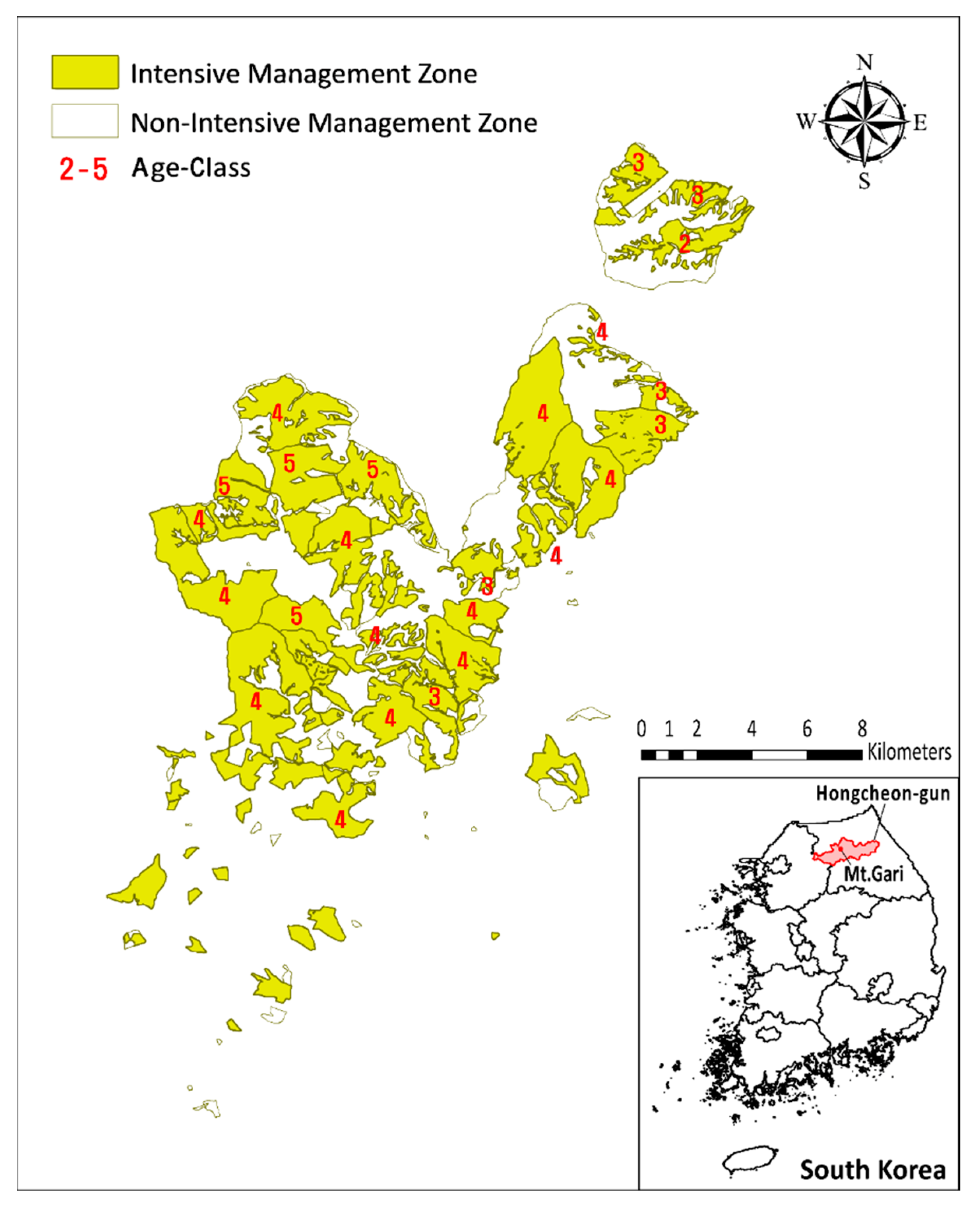
2.1. Study Area

Forests on Mt. Gari, located in Hongcheon-gun, South Korea, were selected as the study area. Hongcheon-gun is a county in Gangwon Province, located on the east side of the central part of the Korean Peninsula. The county, with a total area of 1820.3 km2, is the largest among cities and counties in the country.
Since 2013, the Korea Forest Service (KFS) has designated leading forest management complexes (LFMCs) throughout the country. These complexes’ purpose is to systematically manage forests to maximize investment returns by developing a successful forest management model based on long-term plans. Five national and 21 private forests are operating as LFMCs as of 2021 [28]. The forests at Mt. Gari were designated national LFMC in 2012 and administrated by the Hongcheon National Forest Management Office.
Mt. Gari LFMC covers an area of 6636 hectares and is divided into an intensive management zone and a non-intensive management zone. The intensive management zone was set by excluding areas where it was difficult or impossible to perform forest operations (Figure 3). The area of the intensive management zone is 4480 hectares and comprises 25 compartments and 495 sub-compartments. The average elevation of each sub-compartment ranges from 300 to 900 m, and the slope varies from sub-compartment to sub-compartment.
Planted forests account for 82% and natural forests account for 18%. The average forest growth stock is 164 m3 per hectare. The primary tree species are Pinus koraiensis Siebold & Zucc. and Larix kaempferi (Lamb.) Carrière, with Pinus koraiensis and Larix kaempferi accounting for approximately 36% and 33%, respectively. In addition to these tree species, there are also other conifers and broad-leaved trees. The zone age class distribution is highly unbalanced, with forest stands older than 31 years accounting for approximately 86%, as shown in Table 1 [29].

2.2. Forest Management Planning Model

MOLP is a mathematical programming model that solves complicated problems requiring simultaneous consideration of multiple conflicting values. In forestry, the MOLP has been consistently used to establish multi-objective long-term management plans for large forest areas. This study utilized the MOLP-based forest management planning model developed by Kim et al. [22] to analyze the economic and ecological impacts of variations in timber production on forest management from a long-term perspective.
The model’s primary objective was to maximize the sum of the weighted net present value (NPV) of timber production, carbon storage, and water storage over the entire planning horizon (i.e., 150 years) (Equation (1)). The NPV of timber production was determined by referring to the Hongcheon National Forest Management Office’s timber sales and silvicultural prescription cost records from 2013 to 2018 (Table 2) and was calculated by subtracting total cost of timber production (thinning and final cutting) from total profit obtained by timber sales for each period. The carbon storage NPV was calculated by multiplying the carbon storage amount by the Korea Offset Credits (KOC) average price in US dollars from 2016 to 2021. Finally, the NPV of water storage was predicted by multiplying the amount of water stored by the cost of storing the same amount in the dam (i.e., the dam construction cost).
The equation used to calculate the objective function is as follows:
max   w t { p i b j a ( t r p × V T p t c p ) × Z i b j a + p i b j a ( h r p × V H p h c p ) × Z i b j a } + w c p i b j a C p × Z i b j a + w w p i b j a W p × Z i b j a
where V T p and V H p are timber production volume from thinning and final cutting at period p , respectively. t r p and h r p indicate the NPV values of timber sales per m3 while t c p and h c p represent the NPV values of timber production cost per unit area. C p and W p are functions calculating the NPV values of carbon and water storage at period p ; w t , w c , w w represent the respective weights for timber production, carbon storage, and water storage, respectively. The decision variable used in the model is Z i b j a , which is the area where species b was planted in period i, cut, and regenerated to species a in period j in zone Z.
Forest inventory data from Mt. Gari and a stand-yield table [30] were used to project timber production volumes. The carbon storage quantity was obtained by multiplying the growing stock by the carbon emission factors for each species, as developed by Son et al. [31]. Water storage amounts were calculated by applying Kim et al.’s [32] formula for porosity calculation, which uses each stand area’s average soil depth considering age class and type—for example, planted versus natural forest types. The same weight was applied to each term of NPVs in Equation (1) assuming that the values of timber production, carbon storage, and water storage are treated equally in the study area. The sets, decision variable, and parameters used in the MOLP formulation are given in Table 3.
The model has eleven constraints expressed by the following equations:
i b j = p a = s Z i b j a i = p b = s j a Z i b j a = 0         f o r   i , j P ,   a , b S
( 1 α ) × H p 1     H p     ( 1 + β ) × H p 1           f o r   p P
A C k p     γ k p × A R E A           f o r   k K ,   p P
δ s p × A R E A     A s p     ε s p × A R E A         f o r   s S ,   p P
ζ z p × A R E A     C A z p     η z p × A R E A         f o r   Z Z ,   p P
θ z p × A R E A     B A z p     ι z p × A R E A         f o r   Z Z ,   p P
V T p     L V T p         f o r   p P
V H p     L V H p         f o r   p P
t r p × V T p     L T R p         f o r   p P
h r p × V H p     L H R p         f o r   p P
Z i b j a     0         f o r   i , j ,   a ,   b
where, α is the allowable decreasing rate in timber production. β is the allowable increasing rate in timber production. A R E A is the total area of the forest. At period p , A C k p is the area of age-class k and γ k p is the lower bound area of age-class k. A s p is the area of species s, δ s p is the lower bound area of species s, and ε s p is the upper bound area of species s at period p . C A z p is the area of conifers at period p in zone z. ζ z p is the lower bound area and η z p is the upper bound area of conifers at period p in zone z. B A z p is the area of broad-leaved trees at period p in zone z. θ z p is the lower bound and ι z p is the upper bound area of broad-leaved trees at period p in zone z. V T p is the timber production from thinning and L V T p is the target timber production from thinning at period p . V H p is the timber production from final cutting and L V H p is the target timber production from final cutting at period p . t r p is the timber sales from thinning per m3 and L T R p is the target timber sales from thinning at period p . H R p is the timber sales from final cutting per m3 and L H R p is the target timber sales from final cutting at period p .
Equation (2) expresses the assumption of reforestation within the same period after the final cutting, indicating that the area of species planted in period p is the same as the area harvested at period p and regenerated to species s. Equation (3) narrows the period-to-period variation rate in timber production. Equation (4) is used to adjust the age-class structure by setting the minimum percentage of the area occupied by each age class in each period. In Equation (5), each species’ minimum and maximum percentages were set to control their composition. Equations (6) and (7) were used to set the minimum percentage of conifers and broad-leaved trees in each management zone to reflect the differences in management objectives between zones. Equations (8) and (9) express the constraints on the minimum timber production from harvest in each period, and Equations (10) and (11) express the constraint on the minimum timber sales amount from the harvest in each period.
This study focused on limiting the rate of variation in timber production (Equation (3)) among the constraints of the MOLP-based forest management planning model. The silvicultural prescription scenarios and input values for each constraint are given in Table 4 and Table 5. The entire study area was divided into three forest functions; those functions and six tree species were combined in determining the timing of timber harvests in prescription scenarios (Table 4). The strategic broad-leaved trees referenced in Table 4 denote the species utilized in planned afforestation, including five broad-leaved tree species: Fraxinus rhynchophylla, Juglans mandshurica, Cornus controversa, Betula platyphylla, and Fraxinus mandshurica [29]. The objective function was to maximize the NPV of forest management by considering timber production, carbon storage, and water storage in equal proportions during the entire planning horizon.

2.3. Sensitivity Analysis

A sensitivity analysis was performed to analyze changes in the total volume and NPV of timber production, carbon storage, and water storage, as well as species and age-class distributions according to the variation rate in timber production. Management alternatives were constructed by varying the rate of timber production. A total of nine management alternatives were identified by setting a standard alternative with limitless period-to-period timber production variation rates and by reducing timber production rates by 5% within a 50% to 15% range (Table 6). The total volume and NPV of timber production, carbon storage, and water storage were compared for each management alternative to determine each alternative’s economic and ecological impacts.

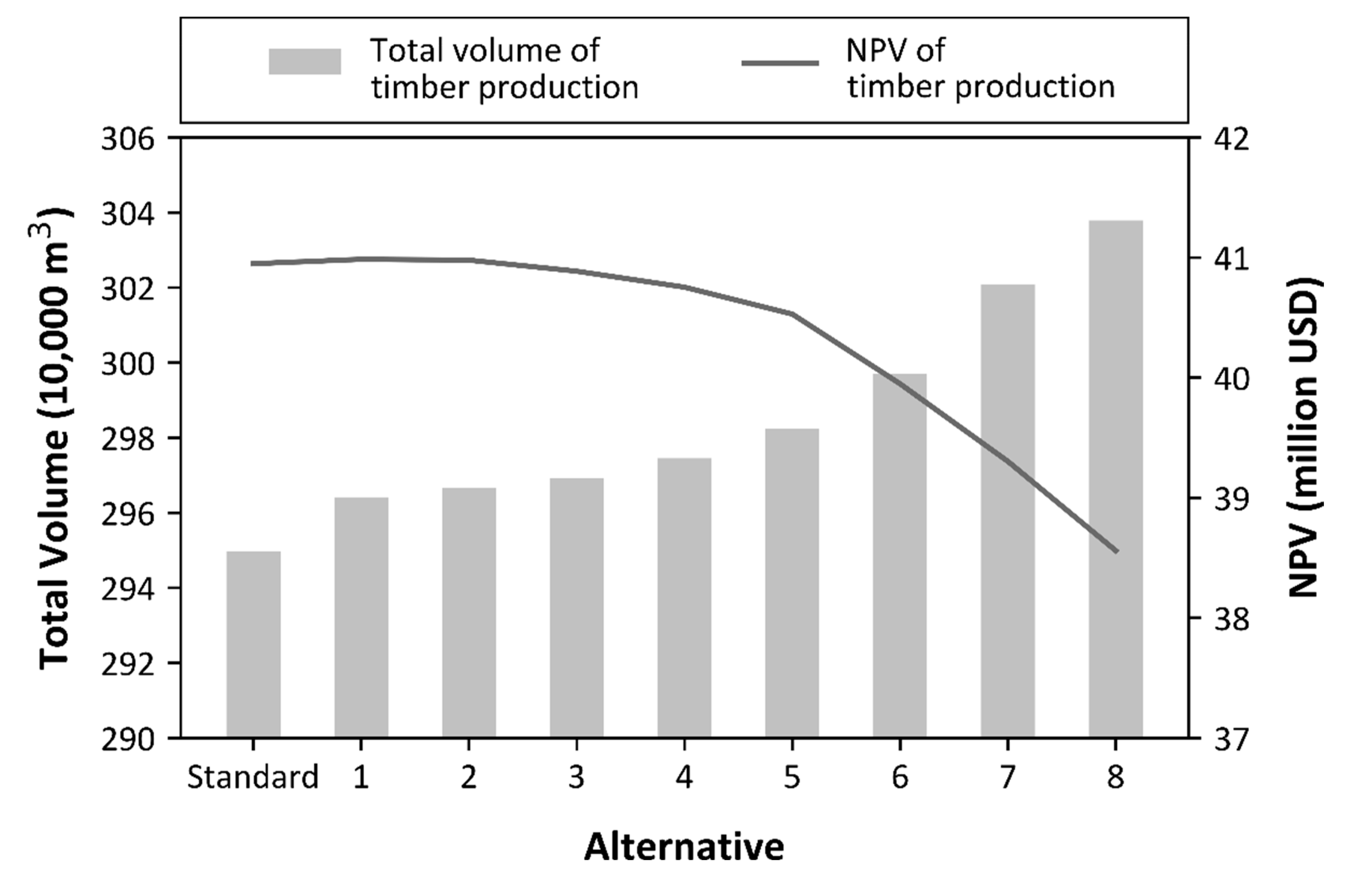
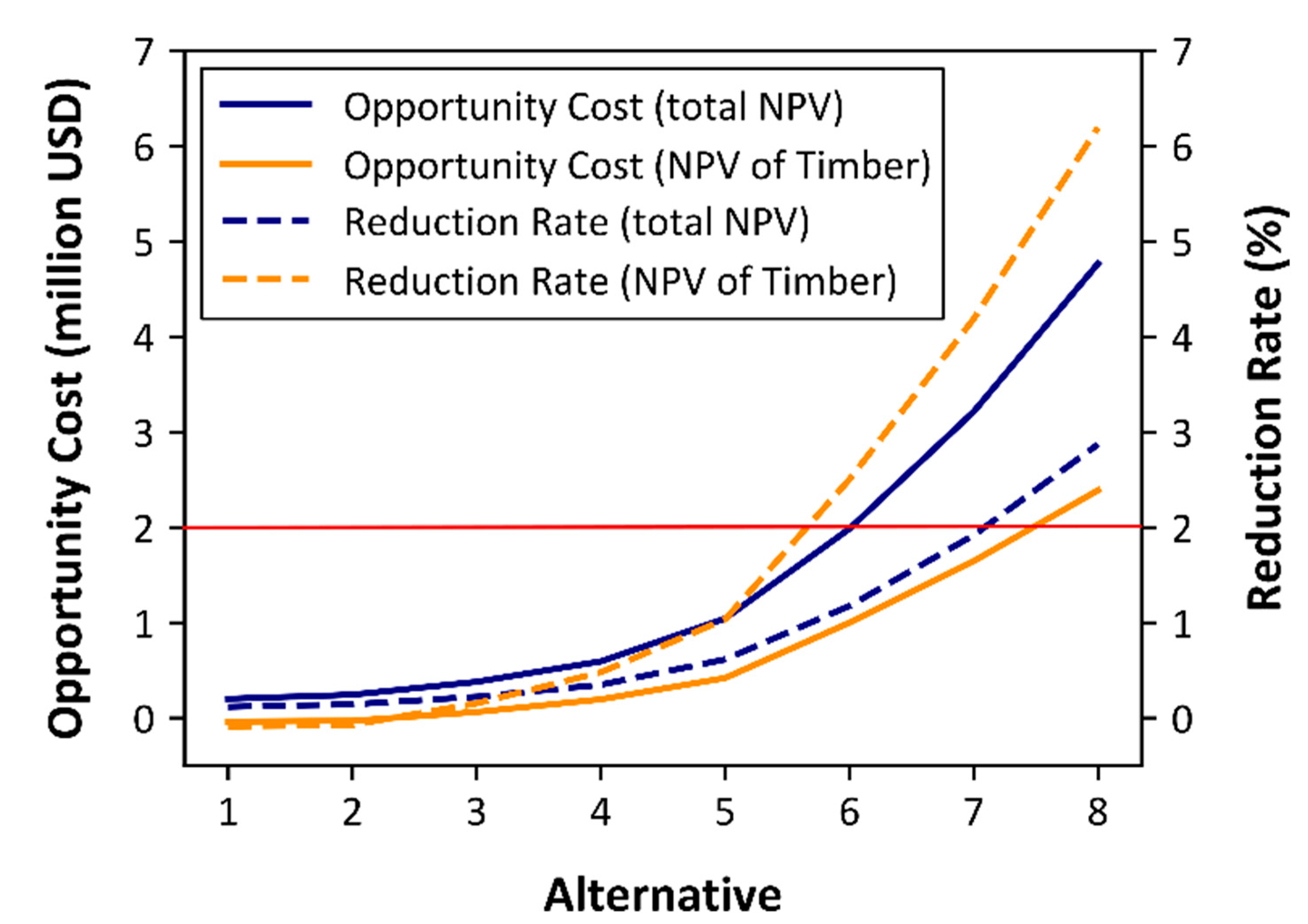
2.4. Determination of Appropriate Variation Rate in Timber Production

The stability of timber production might increase if the variation rate in timber production is strictly limited. However, there are trade-offs between timber production stability and other ecological benefits. This study determines the most appropriate management alternative with balanced timber production and ecological benefits such as carbon and water storage.
The most appropriate alternative was identified by calculating opportunity costs like NPV decreases and NPV values reduction rates compared to the standard alternative. We set the allowable reduction rate of the NPV to 2% and calculated the opportunity costs and reduction rates using the NPV sum of timber production, carbon storage, and water storage and the NPV sum of timber production alone. After determining the most appropriate alternative, age-class distribution changes and forest tree species composition were projected using the forest management planning model.

3. Results and Discussion

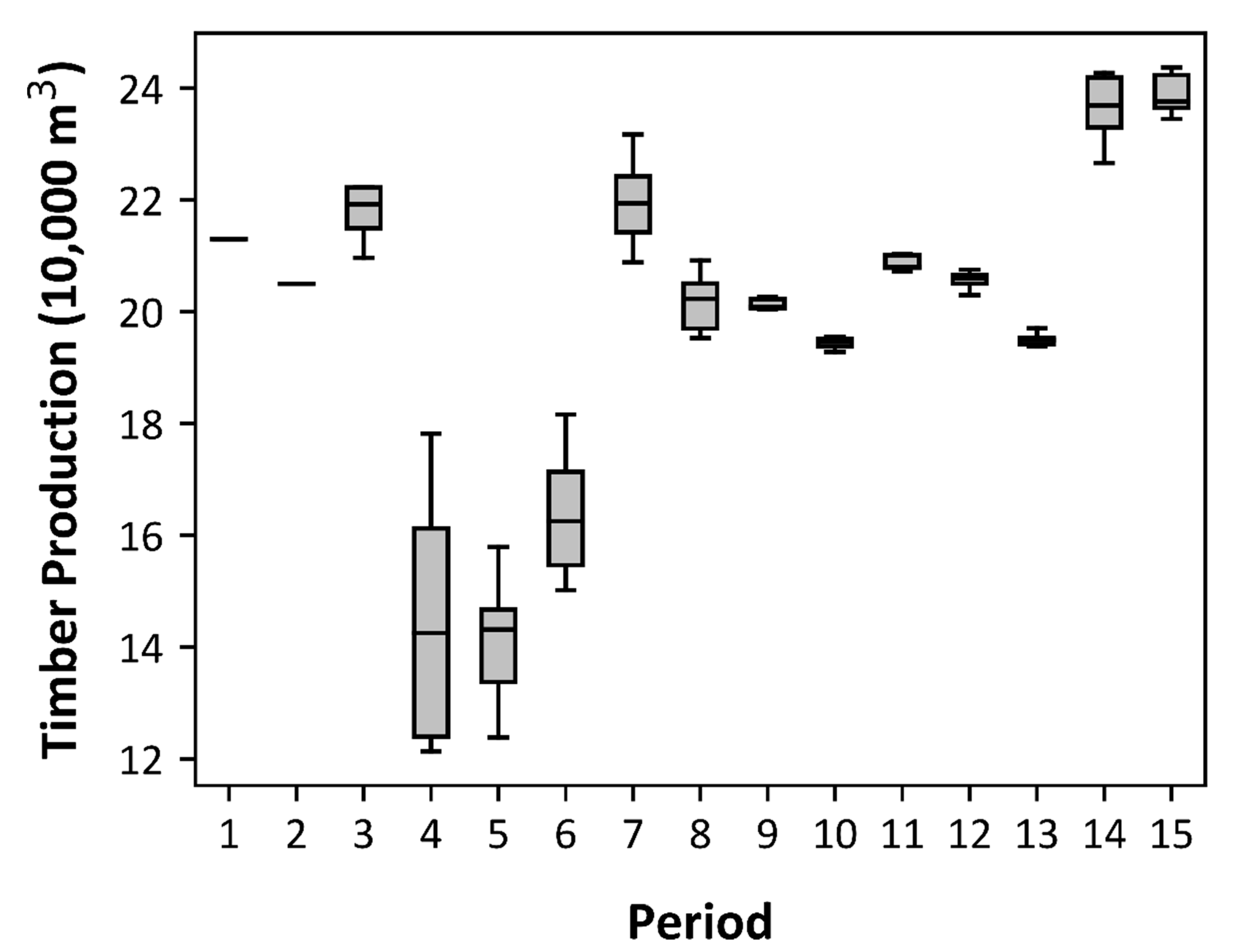
3.1. Changes in Timber Production

Figure 4 shows the total volume and NPV of timber production harvested during the entire planning horizon for each management alternative. As timber production variation rates lessened, the total volume of timber production increased. In addition, between alternatives, while the total volume of timber production increased, timber production net present value (NPV) decreased except for a minor increase (0.09%) between the standard and first alternatives.
At Mt. Gari, about 86% of the current stands are over 31 years old, so large harvest amounts occurred during the first to third periods. Figure 5 shows that the difference in timber production by alternative occurred mainly between the third and eighth periods. This means that the intensity of adjustment for age class structure varied depending on the different variation rate of timber production by alternatives during those periods. A relatively large change in the amount of timber production was modelled to balance age class structure in alternatives with high variation rate, while a small change in the amount of timber production was only permitted in alternatives with high restriction on timber production in the same period of time. As the age class is balanced toward the latter part of the planning periods, however, the need for such a large change in the amount of timber production among alternatives decreases. This time range up to the 8th period was a conversion period where the current forest age-class structure converted into the target age-class structure.
The constraint on the period-to-period variation in timber production influenced the regeneration species selection at the beginning of the planning period. For example, when there were tight constraints on timber production variation rates, the tree species Pinus rigida was planted at a high rate during the conversion period to reduce the gap in the harvested amounts in subsequent periods (Figure 6). Pinus rigida grows rapidly and has a short rotation age; thus, the total volume of timber production increased. However, the economic value of timber production decreased because the timber price of Pinus rigida was lower than that of the other species (Table 2).
This selection changed timber production’s volume and economic value during the planning horizon. The stronger the constraint on the variation in timber production, the greater the regeneration of Pinus rigida, which caused a decrease in economic value. Suppose the timber price of Pinus rigida is raised; it may raise the economic value while maintaining timber production stability. In such cases, however, it also needs to be considered whether Pinus rigida play an ecologically important role in the region if we want to select it as a regeneration species.

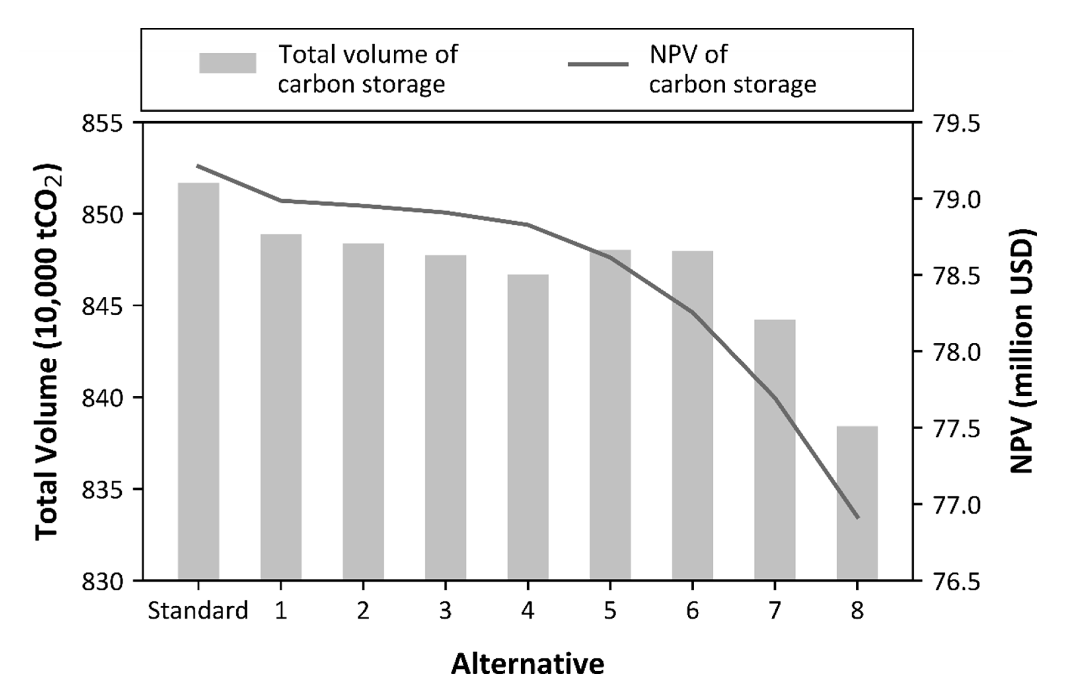
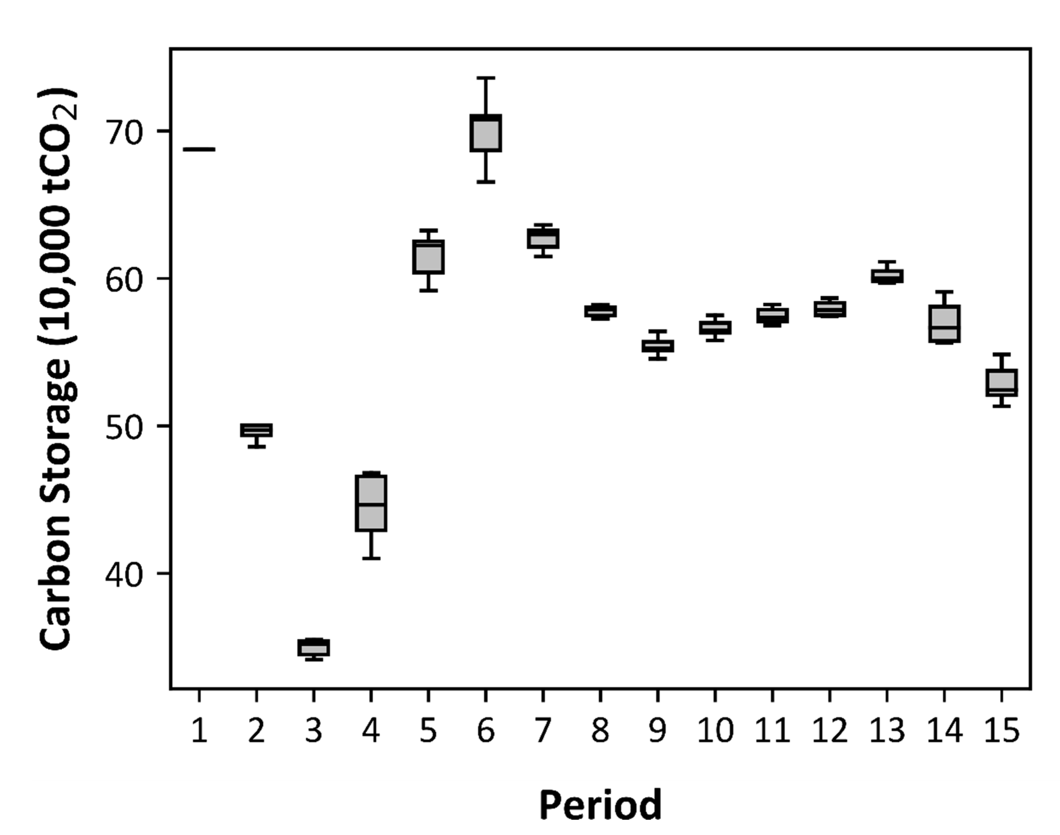
3.2. Changes in Carbon Storage

As the variation rate in timber production lessened, the total volume of carbon storage decreased, except for the increase between alternatives 4 and 5 and alternatives 4 and 6 (Figure 7). A difference was mainly found in the conversion period to adjust the age-class structure, similar to timber production (Figure 8). The amount of stored carbon is affected by the forest growing stock. The stronger the constraint on timber production variation rate, the higher the frequency and amount of harvest increased as the proportion of Pinus rigida increased during the conversion period, reducing the relative carbon storage volume in forests. As the timber production variation rate lessens, the carbon storage at the beginning of the planning horizon also lessens.
In the latter part of the planning horizon, the differences between alternatives caused by timber production variation rates decreased. Consequently, there was a reduced burden to adjust the age-class structure, tree species selection, and silvicultural prescriptions. For example, the area of broad-leaved trees with excellent carbon absorption and water storage capacity increased during the latter part of the planning horizon (Figure 9).

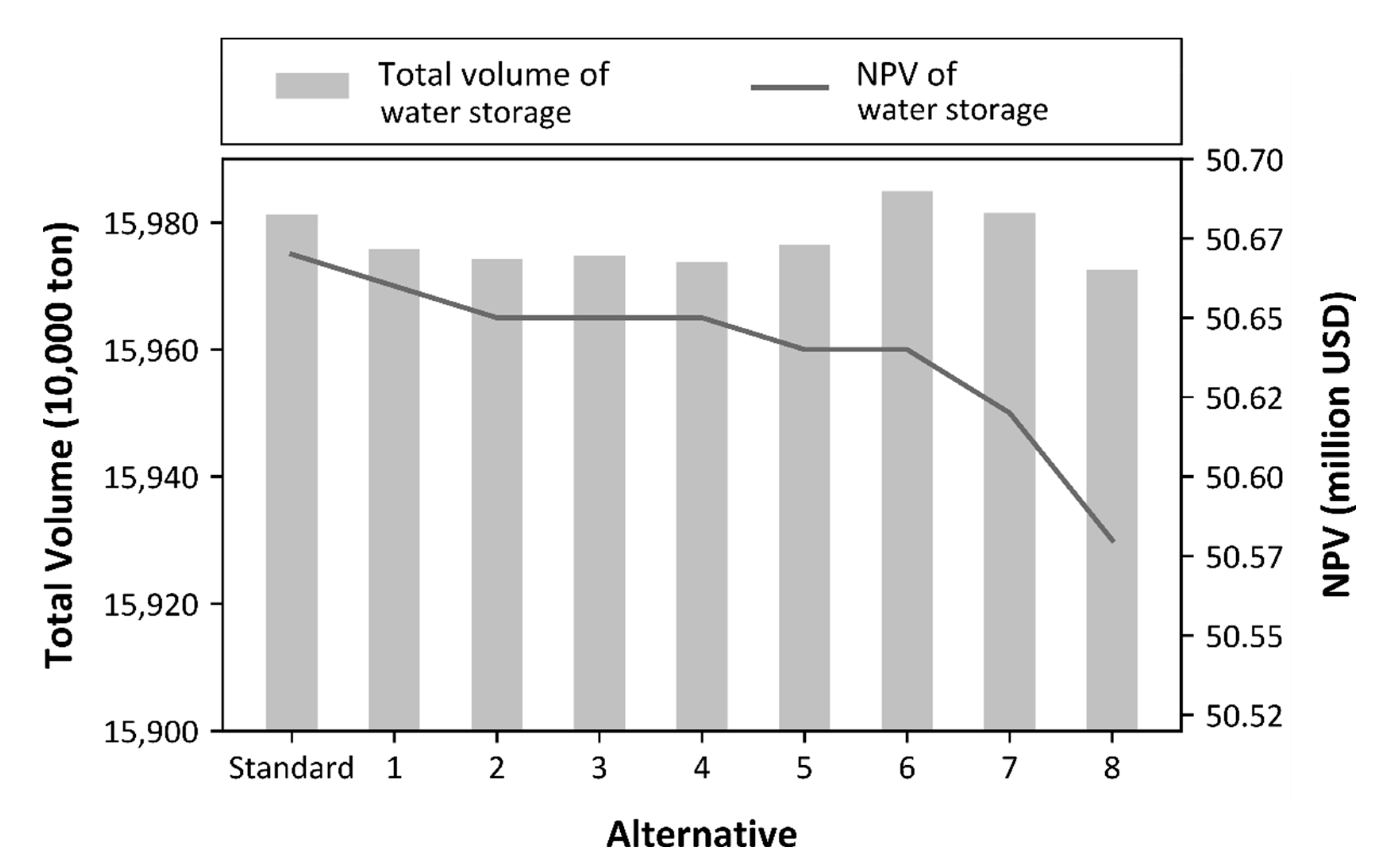
3.3. Changes in Water Storage

The volume of water storage fluctuated with the variation rate in timber production, and the NPV decreased with stricter constraints on the variation rate (Figure 10). The difference in the NPV of water storage by alternative was relatively small compared to the difference in NPV of timber production and carbon storage, as can be seen from the low coefficient of variation (CV) in Table 7. Furthermore, water storage volume over time was not significantly different between alternatives (Table 8). Thus, water storage was less affected by the forest tree species selection and silvicultural prescriptions compared with timber production and carbon storage.

3.4. Appropriate Variation Rate in Timber Production

Figure 11 shows the opportunity costs incurred by limiting the variation rate in timber production for each management alternative and the reduction rates of the NPV values compared to the standard alternative. As timber production variation restrictions rose, opportunity costs and reduction rates increased. In addition, the difference between alternatives tended to increase rapidly, beginning at alternative 5, which limited the timber production variation rate to 30%. Forest managers can choose the best-fit alternative with a high economic value from forest management and low timber production variation rates by setting an allowable threshold for opportunity cost or reduction rates.
This study set the allowable reduction rate of the NPV values to 2%. Alternatives 1–5 were within the NPV values reduction rate threshold. Therefore, alternative 5, which had the lowest timber production variation rate and guaranteed the highest timber production stability, was selected as the most appropriate alternative for the management of the forest.

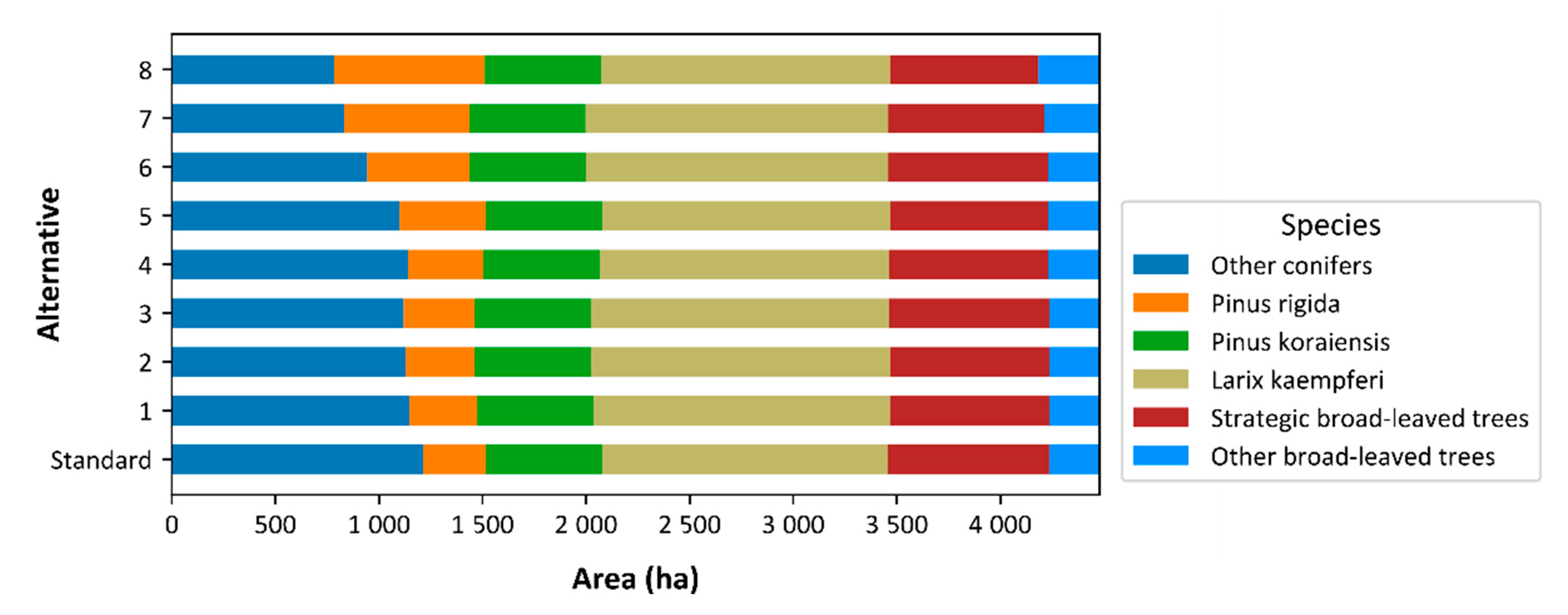
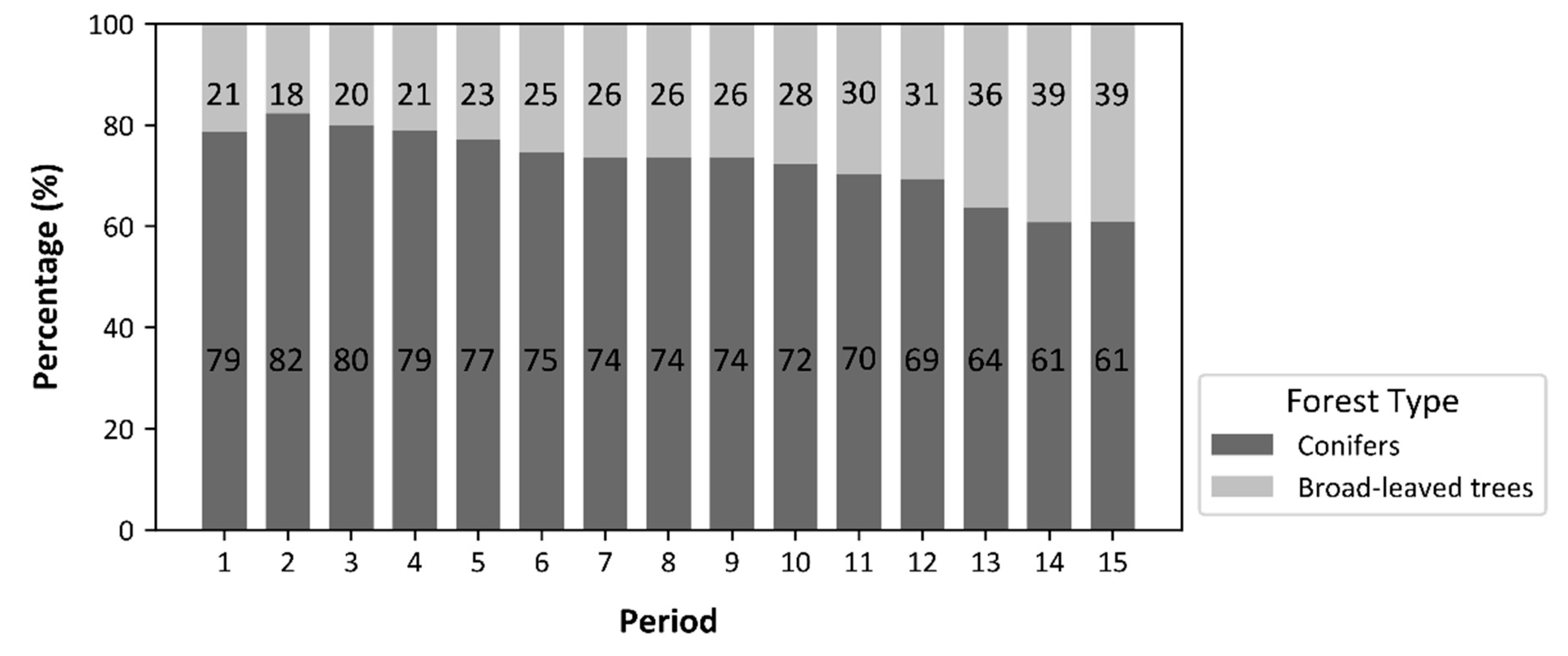
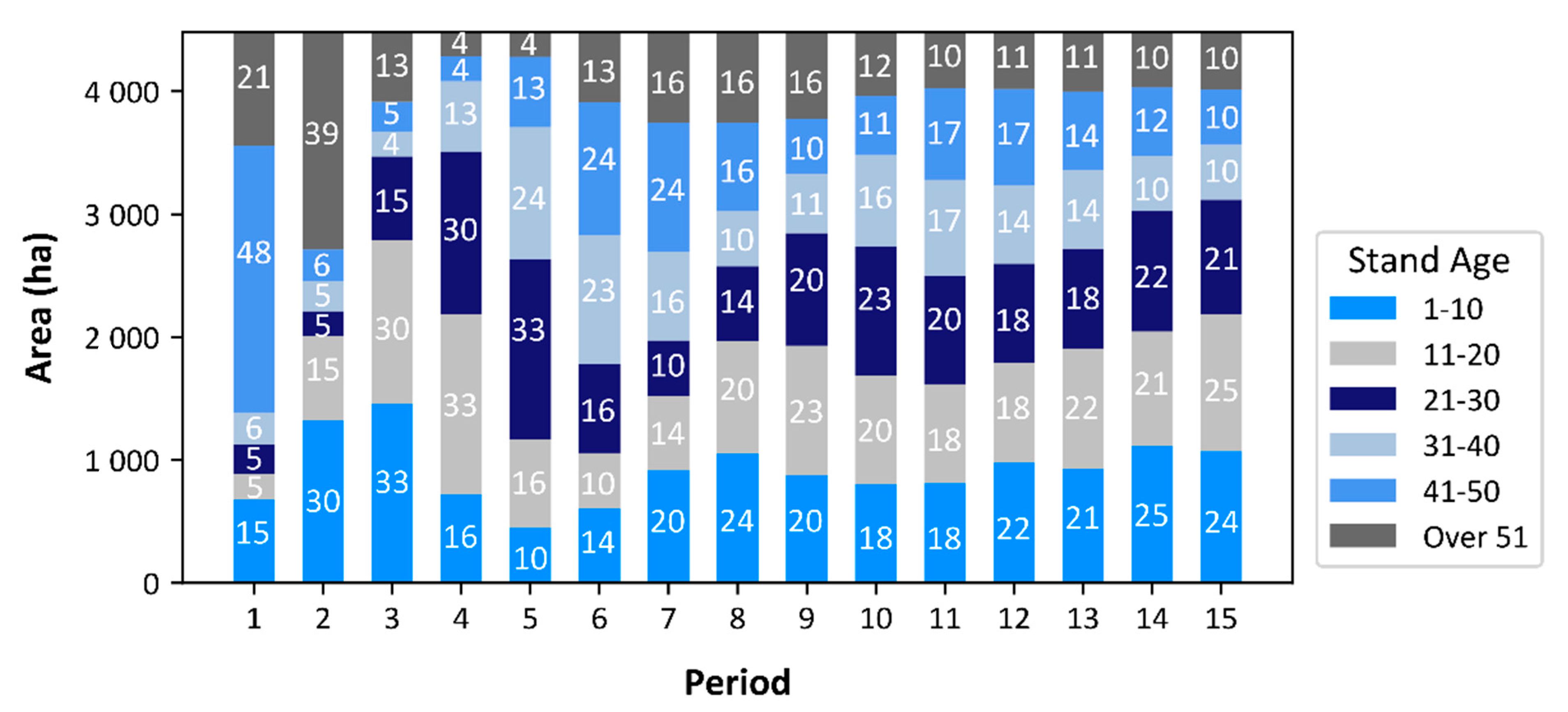
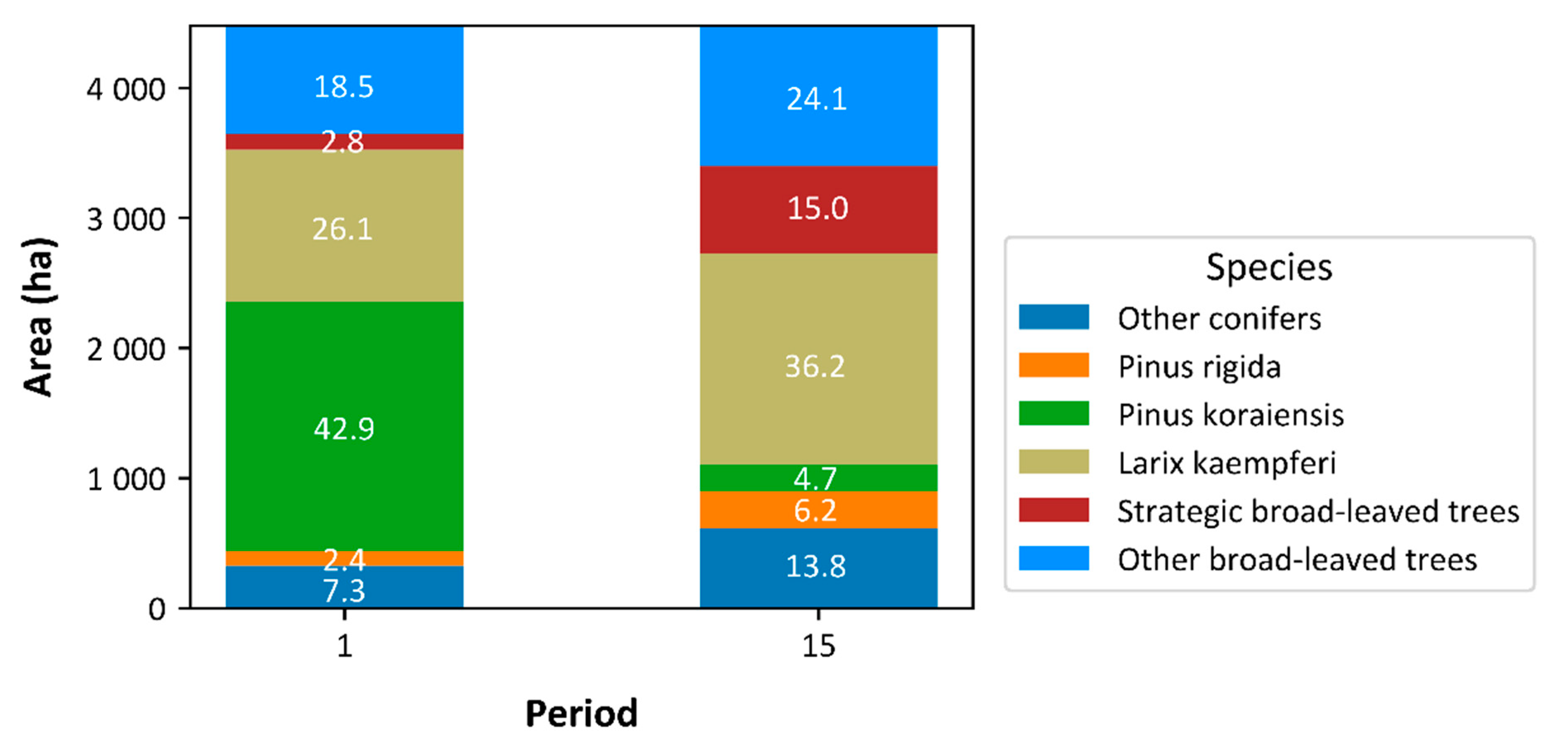
3.5. Changes in Age-Class Distribution and Species Composition

Figure 12 shows the projected changes in the age-class structure for each period when we applied the most appropriate timber production variation rate to the forest planning model. Currently, forest stands exceeding 31 years occupy most of the area, but the distribution will be balanced gradually through planned harvest and regeneration. Therefore, the forest stand area in each age class is expected to be evenly distributed according to the constraint, and the distribution of age class becomes relatively balanced after the eighth planning period.
Tree species composition also varied according to the area of the target species at the end of the planning horizon set in the constraint. The planning model caused the area of Pinus koraiensis to decrease compared with the current stand, while the area of Larix kaempferi and broad-leaved trees increased (Figure 13). There are currently plans to reduce the area of Pinus koraiensis on Mt. Gari owing to damages from the rapid spread of pine wilt disease. Post plan application, the Pinus koraiensis area will be reduced from 1613 hectares, 42.9% of the area in period 1, to 210 hectares, 4.7% of the area in period 15. Conversely, the area of the broad-leaved tree has increased because of its high carbon and water storage capacity. Strategic broad-leaved trees were planned to increase the area; thus, there was a significant increase from 82 hectares (2.8% of the area) in period 1 to 672 hectares (15.0% of the area) in period 15.

4. Conclusions

This study analyzed the economic and ecological impacts of constraining the period-to-period variation in timber production when establishing a long-term forest management plan to adjust the Korean forest age-class structure, where stands of certain age classes occupy a high proportion of the total forests. It was found that, depending on the variation rate in timber production, the age-class structure and species composition changes, affecting the forests’ economic and ecological functions, including timber production and carbon and water storage. This study determined that short-rotation forestry can be applied to resolve the problem of age-class imbalance in South Korea.
However, the total volume of carbon storage and the NPV of carbon storage and water storage tended to decrease as the range of the variation rate in timber production narrowed. The latter was influenced by an increase in the area of short-rotation species. On the other hand, there was no particular tendency in total volume of water storage according to the difference in variation rate, and water storage was less affected by the selection of species and prescriptions compared to timber production and carbon storage.
The effects of lowering timber production profitability due to short rotation must also be considered from an economic perspective. By calculating the opportunity cost and reduction rate of the NPV and setting the allowable criterion, the most appropriate variation rate in timber production was determined to be 30%. This timber production variation rate is significant because it was determined based on the rate’s economic and ecological impacts on the forests from a long-term forest management plan. Therefore, it is expected that the results of this study will help transform the forest age structure to achieve a balanced age-class distribution and establish a sustainable forest management system in the country.
In order for the results of this study to be effectively applied to national forest management, however, it is necessary to further analyze changes in the age class structure and other forest functions through timber production for a larger area of forest as well as the owner type and/or governance that affects forest management decisions.

Author Contributions

Conceptualization, D.K. and H.H.; methodology, D.K. and Y.K.; validation, D.K. and J.S.; formal analysis, D.K.; investigation, D.K. and H.H.; resources, H.H. and Y.C.; writing—original draft preparation, D.K.; writing—review and editing, H.H. and Y.K.; visualization, D.K. and J.S.; supervision, H.H.; project administration, H.H.; funding acquisition, H.H. All authors have read and agreed to the published version of the manuscript.

Funding

This work was supported by the New Faculty Startup Fund from Seoul National University.

Institutional Review Board Statement

Not applicable.

Informed Consent Statement

Not applicable.

Data Availability Statement

Not applicable.

Conflicts of Interest

The authors declare no conflict of interest.

References

  1. Korea Forest Service. Statistical Yearbook of Forestry; Korea Forest Service: Daejeon, Republic of Korea, 2020. [Google Scholar]
  2. Jun, M.S.; Jeong, Y.H.; Kim, M.S. Dense and Aging Forests, Paradigm Shift in the Management; Policy Press, Research Institute for Gangwon: Chuncheon, Republic of Korea, 2020. [Google Scholar]
  3. Kim, K.D.; Bae, J.S.; Yim, J.S.; Han, H.; Lee, S.J.; Choi, H.T.; Lee, C.W.; Lee, C.H.; Kim, R.H.; Park, C.R.; et al. The Results of the Evaluation of Forest Public Function and the Implication; Korea Forest Research Institute: Seoul, Republic of Korea, 2020; Volume 2018. [Google Scholar]
  4. Böttcher, H.; Kurz, W.A.; Freibauer, A. Accounting of forest carbon sinks and sources under a future climate protocol—Factoring out past disturbance and management effects on age-class structure. Environ. Sci. Policy 2008, 11, 669–686. [Google Scholar] [CrossRef]
  5. Won, H.K.; Kim, Y.H.; Kwon, S.D. Estimation of optimal harvest volume for the long-term forest management planning using goal programming. J. Korean Soc. For. Sci. 2009, 98, 125–131. [Google Scholar]
  6. Curtis, F.H. Linear programming and the management of a forest property. J. For. 1962, 60, 611–616. [Google Scholar]
  7. Leak, W.B. Estimating Maximum Allowable Timber Yields by Linear Programming; United States Forest Service: Washington, WA, USA, 1964; Volume 17. [Google Scholar]
  8. Kidd, W.E.; Thompson, E.F.; Hoepner, P.H. Forest regulation by linear programming—A case study. J. For. 1966, 64, 611–613. [Google Scholar]
  9. Nautiyal, J.C.; Pearse, P.H. Optimizing the conversion to sustained yield—A programming solution. For. Sci. 1967, 13, 131–139. [Google Scholar]
  10. Kwon, O.B. Timber yield regulation using linear programming. J. Agric. Life Environ. Sci. 1969, 3, 25–31. [Google Scholar]
  11. Cho, E.H. A study on the forest yield regulation by systems analysis. Korean J. Agric. Sci. 1977, 4, 344–390. [Google Scholar]
  12. Johnson, K.N.; Scheurman, H.L. Techniques for prescribing optimal timber harvest and investment under different objectives—Discussion and synthesis. Forest Sci. 1977, 23, a0001–z0001. [Google Scholar]
  13. Johnson, K.N.; Jones, D.B. A User’s Guide to Multiple Use—Sustained Yield Resource Scheduling Calculator (MUSYC), Timber Management; United States Forest Service: Fort Collins, CO, USA, 1979. [Google Scholar]
  14. Kowero, G.S.; Dykstra, D.P. Improving long-term management plans for a forest plantation in Tanzania using linear programming. For. Ecol. Manag. 1988, 24, 203–217. [Google Scholar] [CrossRef]
  15. García, O. Linear programming and related approaches in forest planning. N. Z. J. For. Sci. 1990, 20, 307–331. [Google Scholar]
  16. Woo, J.C. Timber Harvest Scheduling of a Korean pine stand—Forest Management Planning by Linear Programming. J. Korean For. Sci. 1991, 80, 427–435. [Google Scholar]
  17. Başkent, E.M.; Keleş, S. Developing alternative wood harvesting strategies with linear programming in preparing forest management plans. Turk. J. Agric. For. 2006, 30, 67–79. [Google Scholar]
  18. Martin, A.B.; Richards, E.; Gunn, E. Comparing the efficacy of linear programming models I and II for spatial strategic forest management. Can. J. For. Res. 2017, 47, 16–27. [Google Scholar] [CrossRef]
  19. Roise, J.P.; Chung, J.; Lanical, R.; Lennartz, M. Red-cockaded woodpecker habitat and timber management: Production possibilities. South. J. Appl. For. 1990, 14, 6–12. [Google Scholar] [CrossRef] [Green Version]
  20. Chung, J.S.; Park, E.S. An application of linear programming to multiple-use forest management planning. J. Korean For. Sci. 1999, 88, 273–281. [Google Scholar]
  21. Park, E.S.; Chung, J.S. Optimal forest management planning for carbon storage and timber production using multi-objective linear programming. J. Korean For. Soc. 2000, 89, 335–341. [Google Scholar]
  22. Kim, D.Y.; Han, H.; Chung, J.S. Optimal forest management for improving economic and public functions in MT. Gari leading forest management zone. J. Korean For. Sci. 2021, 110, 665–677. [Google Scholar]
  23. Won, H.K.; Kim, H.H.; Chong, S.K.; Woo, J.C. A Forest Management Planning Method based on Integer Programming. J. Korean For. Sci. 2006, 95, 729–734. [Google Scholar]
  24. Costa, P.; Cerveira, A.; Kašpar, J.; Marušák, R.; Fonseca, T.F. Forest management of pinus pinaster ait. in unbalanced forest structures arising from disturbances—A framework proposal of decision support systems (DSS). Forests 2021, 12, 1031. [Google Scholar] [CrossRef]
  25. Cabral, M.; Fonseca, T.F.; Cerveira, A. Optimization of forest management in large areas arising from grouping of several management bodies: An application in Northern Portugal. Forests 2022, 13, 471. [Google Scholar] [CrossRef]
  26. Franklin, J.F.; Johnson, K.N.; Johnson, D.L. Ecological Forest Management; Waveland Press: Long Grove, IL, USA, 2018. [Google Scholar]
  27. Davis, L.S.; Johnson, K.N.; Bettinger, P.S.; Howard, T.E. Forest Management: To Sustainable Ecological, Economic, and Social Values, 4th ed.; McGraw-Hil: New York, NY, USA, 2001. [Google Scholar]
  28. Korea Forest Service. Introduction of Leading Forest Management Complex—Basic Direction. Available online: http://www.sundofm.or.kr/page.php?idx=15 (accessed on 8 October 2021).
  29. Hongcheon National Forest Management Office. The First Comprehensive Plan of MT. Gari Leading Forest Management Complex; Hongcheon National Forest Management Office: Hongcheon, Republic of Korea, 2019; pp. 2019–2068. [Google Scholar]
  30. Kang, J.T.; Son, Y.M.; Jeon, J.H.; Yim, J.S.; Ko, C.U.; Moon, G.H.; Lee, S.J.; Kim, O.S.; Park, Y.J.; Yoon, H.J. The Table of the Stem Volume, Biomass, and Yield; Korea Forest Research Institute: Seoul, Republic of Korea, 2018. [Google Scholar]
  31. Son, Y.M.; Kim, R.H.; Lee, K.H.; Pyo, J.K.; Kim, S.W.; Hwang, J.S.; Lee, S.J.; Park, H. Carbon Emission Factors and Biomass Allometric Equations by Korean Main Species; Korea Forest Research Institute: Seoul, Republic of Korea, 2014. [Google Scholar]
  32. Kim, J.H.; Kim, K.D.; Kim, R.H.; Youn, H.J.; Lee, S.W.; Choi, H.T.; Kim, J.J.; Park, C.R. A Study on the Estimation and the Evaluation Methods of Public Function of Forest; Korea Forest Research Institute: Seoul, Republic of Korea, 2010. [Google Scholar]
Figure 1. Forest growing stock and public value in South Korea since 1960 [1,3]. Between 1987 and 2020, 11 evaluations of South Korean forests’ public value were published.
Forests 13 02144 g001
Figure 2. Age-class distribution of forest stands in South Korea as of 2019 [1].
Forests 13 02144 g002
Figure 3. Location of the Mount Gari Leading Forest Management Complex. Yellow shading indicates the intensive management zone and red numbers indicate the forest stand age-class, as detailed in Table 1.
Forests 13 02144 g003
Figure 4. Total volume and NPV of timber production harvested during the entire planning horizon for each management alternative.
Forests 13 02144 g004
Figure 5. Distribution of timber production volume by alternatives in each period (a period of 10 years). The data in each boxplot include 9 points, representing the volume of timber produced in the period for each alternative.
Forests 13 02144 g005
Figure 6. Average area of each species by alternatives for the first to eighth periods. Strategic broad-leaved trees indicate the species specifically planned to expand afforestation in the master plan of the forest, which include Fraxinus rhynchophylla, Juglans mandshurica, Cornus controversa, Betula platyphylla, and Fraxinus mandshurica.
Forests 13 02144 g006
Figure 7. Total volume and NPV of carbon stored during the entire planning horizon for each management alternative.
Forests 13 02144 g007
Figure 8. Distribution of carbon storage by alternatives in each period. The data in each boxplot include 9 points, representing the carbon storage volume in the period for each alternative.
Forests 13 02144 g008
Figure 9. Proportion of conifers and broad-leaved trees by period.
Forests 13 02144 g009
Figure 10. Total volume and NPV of water stored during the entire planning horizon for each management alternative.
Forests 13 02144 g010
Figure 11. Opportunity cost and reduction rate on the NPV values analyzed by alternatives.
Forests 13 02144 g011
Figure 12. Changes in the age-class distribution for each period with a 30% timber production variation rate. The numbers in the bar graph indicate the area proportions of each age class in the period.
Forests 13 02144 g012
Figure 13. Changes in the tree species composition from the 1st to 15th periods with a 30% timber production variation rate. The numbers in the bar graph indicate the area proportions of each species in the period. Strategic broad-leaved trees denote the species specifically planned to expand afforestation in the forest master plan, including Fraxinus rhynchophylla, Juglans mandshurica, Cornus controversa, Betula platyphylla, and Fraxinus mandshurica.
Forests 13 02144 g013
Table 1. Age-class distribution of forest stands in the study area [29].
Age-ClassStand Age
(Years)
Forest Area
(ha)
Ratio
(%)
11–101974.4
211–202966.6
321–301172.6
431–4083818.7
541–50235652.6
6Over 5167615.1
Total4480100
Table 2. Unit profit and cost of timber harvest by tree species [22].
SpeciesThinningFinal Cutting
Profit
($ per m3)
Cost
($ per ha)
Profit
($ per m3)
Cost
($ per ha)
Pinus koraiensis Siebold & Zucc.482155382183
Larix kaempferi (Lamb.) Carrière572155492346
Pinus rigida Mill.312155232440
Other conifers462155712440
Strategic broad-leaved trees *332155142943
Other broad-leaved trees332155142259
* Strategic broad-leaved trees are species used to expand reforestation in the comprehensive plan for Mount Gari. Fraxinus rhynchophylla Hance, Juglans mandshurica Maxim., Cornus controversa Hemsl., Betula platyphylla Sukaczev, and Fraxinus mandshurica Rupr. are strategic broad-leaved trees.
Table 3. Sets, decision variable, and parameters of the MOLP optimization model.
ElementDescription
Sets
K Set of age classes
P Set of planning periods
S Set of species
Z Set of management zones
Decision variable
Z i b j a Area of species b planted in period i   that harvested and regenerated to species a at period j in zone z (ha)
Parameters
α Allowable decreasing rate in timber production (%)
β Allowable increasing rate in timber production (%)
A R E A Total area of the forest (ha)
A C k p Area of age-class k at period p   ( ha )
A s p Area of species s at period (ha)
δ s p Lower bound area of species s at period p in zone z (ha)
ε s p Upper bound area of species s at period p in zone z (ha)
C A z p Area of conifers at period p in zone z (ha)
ζ z p Lower bound area of conifersat period p in zone z (ha)
η z p Upper bound area of conifersat period p in zone z (ha)
B A z p Area of broad-leaved trees at period p in zone z (ha)
θ z p Lower bound area of broad-leaved treesat period p in zone z (ha)
ι z p Upper bound area of broad-leaved treesat period p in zone z (ha)
V T p Timber production volume from thinning at period p (m3)
L V T p Target timber production volume from thinning at period p (m3)
V H p Timber production volume from final cutting at period p (m3)
L V H p Target timber production volume from final cutting at period p (m3)
t r p Timber sales from thinning at period p ($ per m3)
t c p Timber production costs from thinning at period p ($ per ha)
L T R p Target timber sales from thinning at period p ($)
h r p Timber sales from final cutting at period p ($ per m3)
h c p Timber production costs from final cutting at period p ($ per ha)
L H R p Target timber sales from final cutting at period p ($)
Table 4. Prescription scenarios by forest functions and species, for which timings (year) of thinning and final cutting are presented.
Forest FunctionsArea
(Hectare)
Type of HarvestPinus koraiensis,
Other Conifers,
Strategic Broad-Leaved Trees a,
Other Broad-Leaved Trees
Larix kaempferiPinus rigida
Aesthetic and Ecological process1031Thinning20 yr b, 40 yr20 yr, 40 yr20 yr
Final cutting70 yr60 yr40 yr
Water Conservation264Thinning20 yr, 30 yr, 40 yr20 yr, 30 yr, 40 yr20 yr
Final cutting60 yr50 yr30 yr
Timber production3185Thinning20 yr, 40 yr20 yr, 40 yr-
Final cutting60 yr50 yr30 yr
Total4480
a Strategic broad-leaved trees include Fraxinus rhynchophylla, Juglans mandshurica, Cornus controversa, Betula platyphylla, and Fraxinus mandshurica. b Year.
Table 5. Input values of each constraint applied to the MOLP model. Each value was set according to the first Master Plan of Mount Gari’s Leading Forest Management Complex.
No. of EquationConstraintAttributeInput Value
4Minimum percentage of each age-classAge-class a 115%
Age-class 2–610%
5Minimum percentage of each speciesPinus rigida + Other conifers20%
Larix kaempferi35%
Strategic broad-leaved trees b15%
Other broad-leaved trees3%
Maximum percentage of each speciesPinus koraiensis17%
6Minimum percentage of conifers in each forest functionAesthetic and Ecological process25%
Water Conservation25%
Timber production25%
7Minimum percentage of broad-leaved trees in each forest functionAesthetic and Ecological process25%
Water Conservation50%
Timber production25%
8Minimum timber production from thinning20,000 m3
9Minimum timber production from final cutting150,000 m3
10Minimum timber sales amount from thinning857,000 USD
11Minimum timber sales amount from final cutting5,929,000 USD
a This study used 10-year age class ranges. In other words, age class 1 means 1–10 years, age class 2 means 11–20 years, age class 3 means 21–30 years, age class 4 means 31–40 years, age class 5 means 41–50 years, and age class 6 means 51–60 years, b Strategic broad-leaved trees indicate species specifically planned to expand afforestation in the forest master plan, including Fraxinus rhynchophylla, Juglans mandshurica, Cornus controversa, Betula platyphylla, and Fraxinus mandshurica.
Table 6. Management alternatives with differing timber production variation rates.
AlternativeStandard12345678
Variation Rate in
Timber Production (%)
no limit5045403530252015
Table 7. Coefficient of variation (CV) of the total NPVs of timber production, carbon storage, and water storage by alternatives.
FunctionTimber ProductionCarbon StorageWater Storage
Coefficient of variation (%)2.160.950.05
Table 8. Average variation rate (%) of the volume of each objective (timber production, carbon storage, and water storage) by periods in alternatives.
AlternativeTimber ProductionCarbon StorageWater Storage
Standard19.2614.270.93
113.5513.330.91
213.1913.200.90
311.7013.160.91
412.6413.270.91
511.7112.650.91
610.1612.440.93
79.1311.740.94
87.3911.020.93
Publisher’s Note: MDPI stays neutral with regard to jurisdictional claims in published maps and institutional affiliations.

