A Dynamical Model Based on the Chapman–Richards Growth Equation for Fitting Growth Curves for Four Pine Species in Northern Mexico

Abstract

Tree growth models describe the growth and development of forest ecosystems by considering how the dimensions of each simulated tree change within a certain time. These models have commonly used three growth parameters that describe various biological processes and behaviours, considering a sigmoid growth function: (i) the upper asymptote (θ₁), which is the maximal yield indicated by a final dimension (such as the maximal stem diameter); (ii) the maximum specific growth rate (θ₂), defined as the slope of the tangent at the inflexion point; and (iii) the time elapsed (θ₃), defined by the intercept of this tangent with the abscissas. To the best of our knowledge, however, associations between the three parameters have not been documented for tree species. Using diameter growth data from pine trees located in typical mixed and uneven-aged pine-oak forests in the Sierra Madre Occidental, Mexico, our study aims were: (i) to quantify the putative associations between the three growth parameters and (ii) to test the accuracy of a proposed Hybrid Chapman-Richards growth model based on associations between the three growth parameters, but including only one single parameter, relative to the widely used Generalized Algebraic Difference Approach (GADA) based on the Chapman-Richards, Lundqvist and Hossfeld models and the Hybrid Weibull Model. For statistical comparison of the quality of the models, we used the mean relative percentage error, root mean square error, coefficient of determination and Akaike information criterion to assess the quality of the fit. Although the quality of the five growth models studied was similar, from a practical point of view, the proposed Hybrid Chapman-Richards Model (CR-H) is easier to apply than the other models and has a lower data collection and computational cost. The parameter of CR-H can be easily obtained, by measuring just the dominant trees, especially in coniferous forests with irregular ages. Moreover, in contrast to the Chapman-Richards-GADA factor χ₀, when θ₂ is assumed to be site-specific, the CR-H has always a closed-form solution.

1. Introduction

Tree growth models describe the growth and development of forest ecosystems by considering how the dimensions of each simulated tree change through time, i.e., periodic increment of a tree in response to life processes [1,2] and can be divided into single-tree models (dendrometric variables) and whole stand models that include stand characteristics such as age, size, density, site index and species affiliation and composition [3,4]. These models are used to answer ecological questions, for example, determining the impact of the interdependence between tree species and, their environment on forest development and assessing the forest yields under certain prescribed conditions [1]. Tree growth models are therefore important tools for understanding the dynamics of forest ecosystems and for effective and sustainable forest management [5].

Among others, the Hossfeld [6], Weibull [7], Korf [8] and Richards [9] models are well-known flexible sigmoid growth functions [10,11]. These models have commonly used three growth parameters that describe various biological processes and behaviours: (i) the upper asymptote (${\theta }_1$), which is the maximal yield indicated by a final dimension, as the diameter at breast height (dbh) at the end of the growth stage, (ii) the maximum specific growth rate (${\theta }_2$), which is defined as the slope of the tangent at the inflexion point and (iii) the time elapsed (${\theta }_3$), which is defined by the intercept of this tangent with the t-axis [12]. To the best of our knowledge, however, associations between the three parameters have not been documented for tree species.

Tree growth models are based on height-age or diameter-age relationships for evaluating tree growth, yield potential and site productivity [13]. To avoid the problems inherent to base-age-specific (BAS) site models, Bailey and Clutter [14] simultaneously estimated the site-specific or site-index parameters and the common or global model parameters, using Algebraic Difference Approach (ADA) models. Later, Cieszewski [15,16] proposed the Generalized Algebraic Difference Approach (GADA) models, which allow (and need) more than one parameter to be site specific using at least three growth parameters. GADA produces dynamic site curves with “concurrent” variable asymptotes and polymorphism, and it uses a variety of growth characteristics found across different site qualities. This is why GADA has been widely used for modelling tree growth and site quality in forest yield science [17]. However, GADA also has some weak points, e.g. there is no closed-form solution for the growth intensity factor ${\chi }_0$, when ${\theta }_2$ is assumed to be site-specific in a three-parameter Chapman–Richards model, and therefore neither ${\theta }_1$ nor ${\theta }_3$ can be site specific along with ${\theta }_2$ [15,16,18].

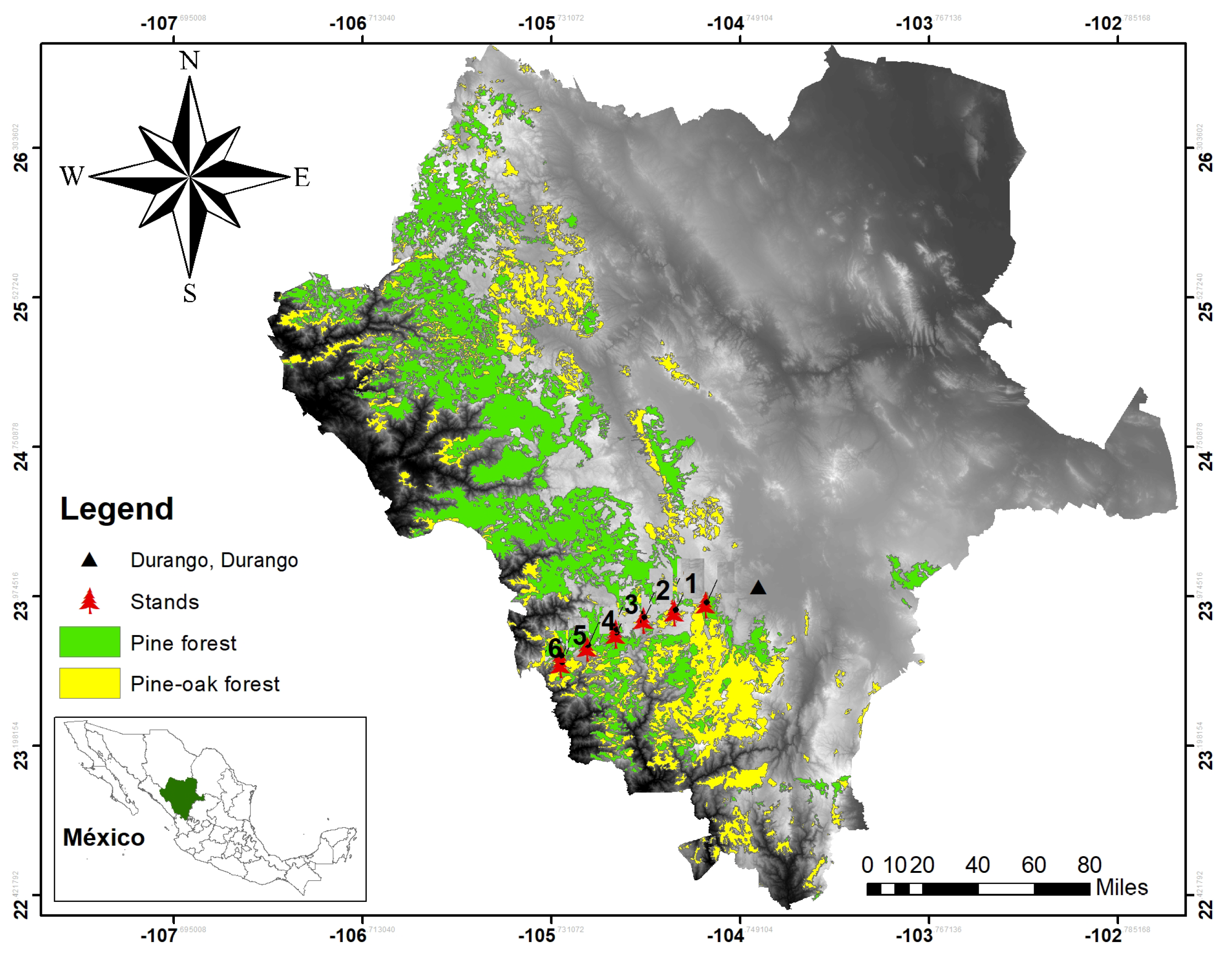
Using diameter growth data from pine trees located in typical mixed and uneven-aged pine-oak forests in the Sierra Madre Occidental, Mexico [19,20], our study aims were: [21] to quantify the putative associations between the growth model parameters and, to test the accuracy of a novel Chapman-Richards growth model, in relation to Hossfeld, Lundqvist and Chapman-Richards GADA models, all with three parameters [22]. Our research results are important for forestry practice, as the new model can be used to predict future yields in a simpler way and with the same accuracy.

2. Materials and Methods

2.1. Sampling Area

The study was conducted between September and November 2017 in a southwest-northeast gradient between the city of Durango, Dgo. and the border of the state o Sinaloa, México, at an elevation range of between 2021 and 2704 m, in different mixed and uneven-aged forests of the Sierra Madre Occidental. Six 50 × 50 m plots were established (0.25 ha), each separated by a distance of 17,000 m in the transect (Figure 1). The diameter at breast height (dbh in cm) at 1.30 m of each tree larger than 7 cm of Pinus arizonica, Pinus engelmannii, Pinus strobiformis and Pinus teocote identified in each plot was measured (

Table 1. Mean diameter at 1.30 m height ($\overline{dbh}$, cm) and respective standard deviation (${\sigma }_{dbh}$), mean age ($\overline{age}$, years) and respective standard deviation (${\sigma }_{age}$) and number of trees (n) of the four pine species in the study.

Species	n	$\overline{\mathit{age}}\pm {\mathit{\sigma }}_{\mathit{age}}$	$\overline{\mathit{dbh}}\pm {\mathit{\sigma }}_{\mathit{dbh}}$
Pinus arizonica	16	$42.75\pm 7.43$	$22.20\pm 6.60$
Pinus engelmannii	97	$36.60\pm 14.58$	$18.26\pm 8.00$
Pinus strobiformis	50	$31.56\pm 10.82$	$13.72\pm 5.13$
Pinus teocote	15	$39.73\pm 11.79$	$29.95\pm 6.81$

). A Pressler borer was used to extract cores (from every tree) at the height of 1.30 m from ground level, and the growth rings were counted (n) and measured to estimate age and increment in diameter [10].

2.2. Generalized Algebraic Difference Approach (GADA) Model

The Algebraic Difference Approach (ADA), introduced by Bailey and Clutter [14], consists of replacing a parameter of the base model with its initial condition solution. The method enables the derivation of dynamic or non-static functions that are capable of producing anamorphic or polymorphic curves, from a Chapman-Richards BAS model chosen a priori.

The GADA methodology [15,16] emerged when it was assumed that two or more parameters of the BAS model are simultaneously site-specific. The Chapman-Richards Hybrid Algebraic Difference Approach (hereinafter CR-H) proposed in this article will be compared with three GADA models widely disseminated in the literature: Chapman-Richards GADA (hereinafter CR-GADA), Hossfeld GADA (hereinafter H-GADA), Lundqvist GADA (hereinafter L-GADA) and one Hybrid Weibull model (hereinafter W-H), presented in the

Table 2. GADA and hybrid equations, where $d_0$ is the diameter (cm) at site-index age $t_0$ (years); $d_r$ is the recruitment diameter at the time $t=0$, which has been considered the same for all individuals; ${\chi }_0$ is a site-specific parameter and ${\theta }_i$ is the parameter associated for each model.

Model	$\mathit{d}\left(\mathit{t}\right)$
CR-GADA	$d\left(t\right)=d_0{\left(\frac{1-e^{-{\theta }_{1}t}}{1-e^{-{\theta }_1{t}_0}}\right)}^{({\theta }_2+{\theta }_3/{\chi }_0)}$ with ${\chi }_0=0.5(ln{d}_0-{\theta }_2{l}_0\pm {({(ln{d}_0-{\theta }_2{l}_0)}^2-4{\theta }_3{l}_0)}^{0.5}$ and $l_0=ln(1-e^{-{\theta }_1{t}_0})$
H-GADA	$d\left(t\right)=\frac{{\theta }_1+{\chi }_0}{1+({\theta }_2/{\chi }_0)t^{-{\theta }_3}}$ with ${\chi }_0=0.5{(d_0-{\theta }_1+({(d_0-{\theta }_1)}^2+4{\theta }_2{d}_0{t}_0^{-{\theta }_3}))}^{0.5}$
L-GADA	$d\left(t\right)=e^{{\chi }_0-({\theta }_1+1/{\chi }_0)t^{{\theta }_3}}$ with ${\chi }_0=0.5({\theta }_1{t}_0^{{\theta }_2}+ln{d}_0+l_0)$ and $l_0={({({\theta }_1{t}_0^{{\theta }_2}+ln{d}_0)}^2+4t_0^{-{\theta }_2})}^{0.5}$
W-H	$d\left(t\right)={\theta }_1-({\theta }_1-d_r){\left(\frac{d_r-{\theta }_1}{d_0-{\theta }_1}\right)}^{-t/t_0}$ with $d_r=0.05$

[15,16,20,23].

2.3. Proposed Hybrid Model Based on a Chapman-Richards BAS Two Parameters model

In the Hybrid Chapman-Richards model proposed here, the number of parameters was first reduced by substituting ${\theta }_2$ by a function, such as ${\theta }_2=f\left({\theta }_1\right)$. In this case, we rewrote the Chapman-Richards BAS model as follows:

$$d\left(t\right)={\theta }_1(1-e^{-{\theta }_{2}t})\Rightarrow {\theta }_1(1-e^{-f\left({\theta }_1\right)t}),$$

(1)

where ${\theta }_1$ is the maximum dbh gotten when the upper asymptote is reached in the individual. This restructuring of the equation restricts the model to just the parameter ${\theta }_1$, although only when the relationship ${\theta }_2=f\left({\theta }_1\right)$ exists and can be established. Then, now considering that we have an inverse relationship between the parameters ${\theta }_1$ and ${\theta }_2$, we can write

$${\theta }_2=a/{\theta }_1,$$

(2)

and it was then possible to rewrite the Equation (1) as

$$d\left(t\right)={\theta }_1(1-e^{-at/{\theta }_1}),$$

(3)

where a is a scale factor. Now, from the ADA methodology, assuming $a={\chi }_0$ to be site-specific in the Equation (3) subject to the initial conditions $d\left(t_0\right)=d_0$, we have

$${\chi }_0=\frac{{\theta }_1}{t_0}ln\left(\frac{{\theta }_1}{{\theta }_1-d_0}\right)$$

(4)

and replacing this result at the Equation (3), we finally have

$$d\left(t\right)={\theta }_1\left(1-{\left(\frac{{\theta }_1}{{\theta }_1-d_0}\right)}^{-t/t_0}\right)$$

(5)

which now depends only on the parameter ${\theta }_1$ under the initial conditions $t_0$ and $d_0$.

2.4. Goodness of Fit of the Models

In order to quantify the error associated with each of the models implemented in the study, we used (because of its robustness and simplicity) the mean absolute percentage error (hereinafter MAPE), here defined as:

$$MAPE=\frac{1}{n}\sum _{i=1}^n\left|\frac{o_i-e_i}{o_i}\right|,$$

(6)

where $e_i$ and $o_i$ are respectively the estimated and the observed values and n is the number of observations.

The root mean square error (hereinafter RMSE) is a measure often used to mark differences between the values predicted by a model and the observed values and is defined as follows:

$$RMSE=\sqrt{\frac{{\sum }_{i=1}^n{(o_i-e_i)}^2}{n}},$$

(7)

where $e_i$ and $o_i$ are respectively the estimated and the observed values, and n is the number of observations.

Finally, the coefficient of determination (hereinafter R²), here defined as follows:

$$R^2=\frac{{\sigma }_{e_i}^2}{{\sigma }_{o_i}^2},$$

(8)

where ${\sigma }_{o_i}^2$ and ${\sigma }_{e_i}^2$ are respectively the variance of the observed and the estimated values.

2.5. Kruskal-Wallis Test

The Kruskal-Wallis test is a non-parametric test used here to indicate whether there is any significant difference between the residuals obtained for each of the models presented in the study (Table 2) compared to the newly proposed hybrid model (CR-H). It is an extension of the Wilcoxon-Mann-Whitney test and is used to test the null hypothesis that all populations have identical distribution functions, against the alternative hypothesis that at least two of them have different distribution functions [24].

2.6. Akaike Information Criterion (AIC)

Akaike information criterion (AIC) [22] is a statistical model selection technique that can be used to compare and select the best model. AIC is based on the likelihood function and penalizes the model with a complexity term. The AIC value for a model is calculated as follows:

$$AIC=-2log\left(L\right)+2k$$

(9)

where L is the likelihood function and k is the number of parameters in the model. The model with the lowest AIC value is considered to be the best model.

2.7. Nonlinear Regression Methods

The algorithm used in the study to fit the models through nonlinear regression methods was implemented in the R language [25] together with the optimization package optimx [26,27], an R package that provides a range of functions for numerical optimization that includes functions for unconstrained and constrained optimization, as well as a wide variety of optimization algorithms.

3. Results

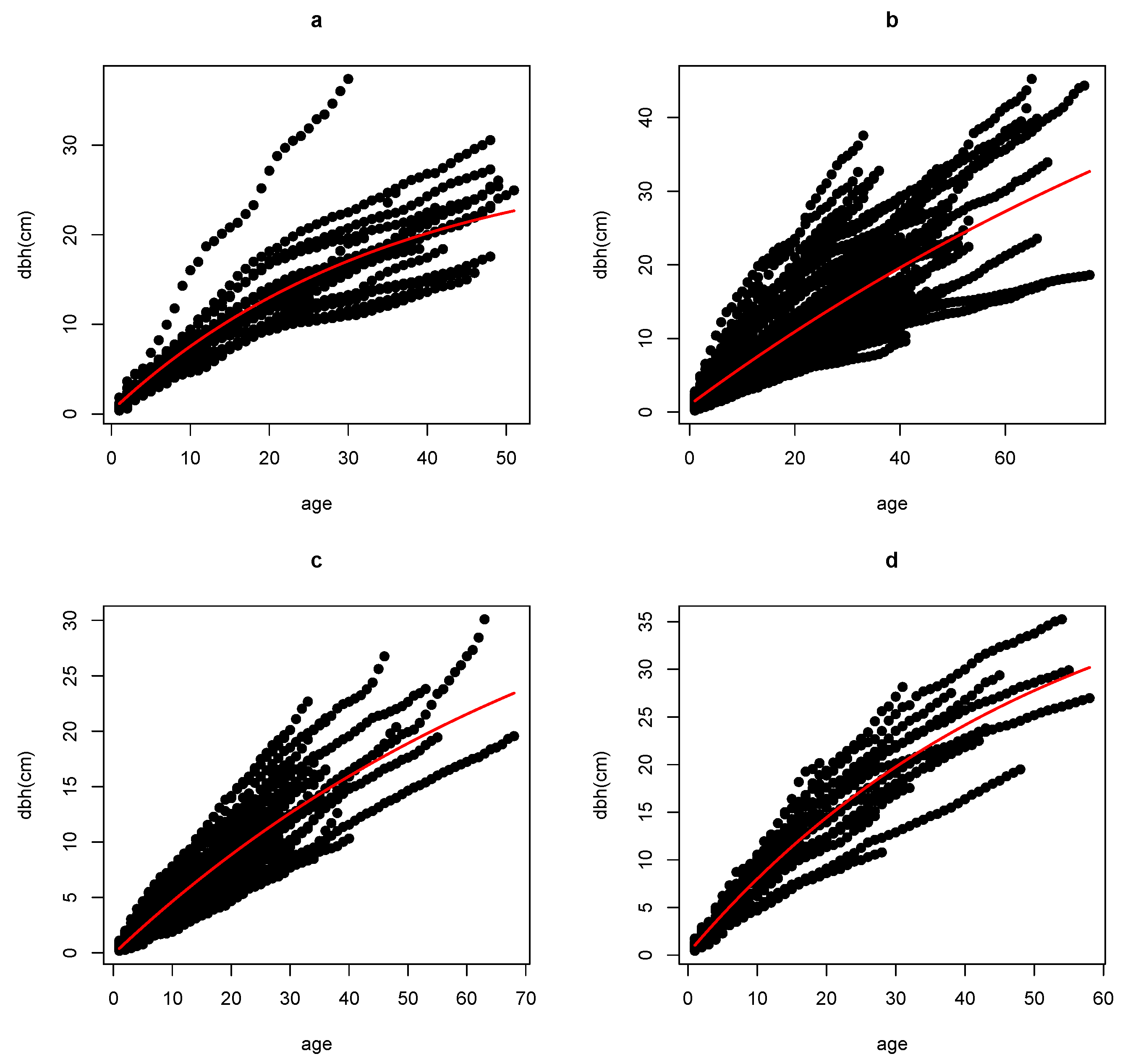
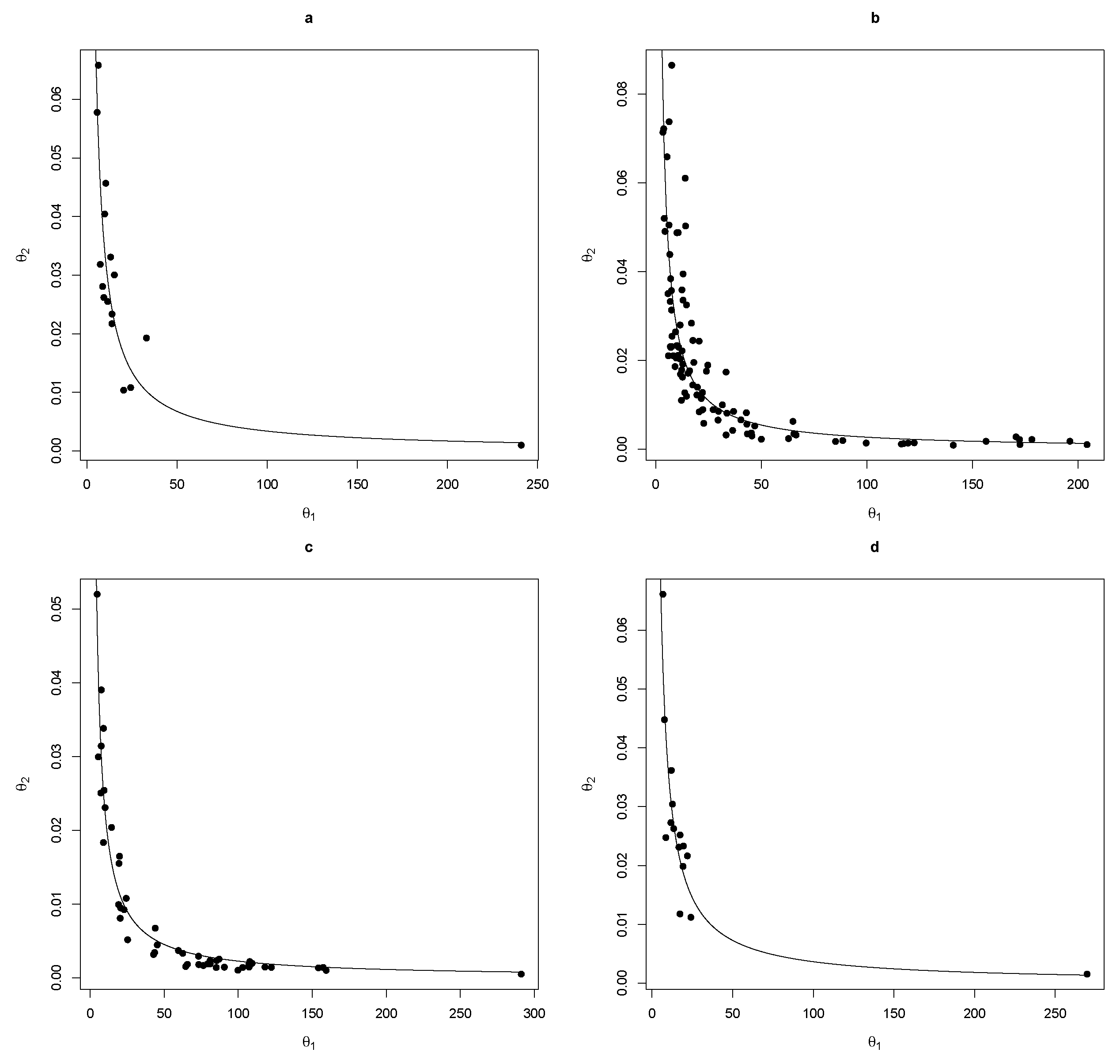
As we can see in Figure 2, the Chapman-Richards BAS model fits very well with the growth history of the species involved in the study. The results show a strong negative relationship between the growth parameters ${\theta }_1$ and ${\theta }_2$ (Figure 3). The scale factor a varied from 0.23–0.34 depending on the tree species. From the adjusted models, it was thus possible to write ${\theta }_2$ as a function of ${\theta }_1$ of the form ${\theta }_2=f\left({\theta }_1\right)=a/{\theta }_1$.

Table 3. Parameters adjusted for the GADA and W-H models in comparison with the CR-H model proposed in the study.

Species	Pinus arizonica			Pinus engelmannii			Pinus strobiformis			Pinus teocote
Model	${\theta }_1$	${\theta }_2$	${\theta }_3$	${\theta }_1$	${\theta }_2$	${\theta }_3$	${\theta }_1$	${\theta }_2$	${\theta }_3$	${\theta }_1$	${\theta }_2$	${\theta }_3$
CR-GADA	2.2 × 10${}^{-3}$	0.45	0.01	1.4 × 10${}^{-4}$	0.03	4.1 × 10${}^{-4}$	9.2 × 10${}^{-7}$	9.1 × 10${}^{-1}$	7.8 × 10${}^{-3}$	9.4 × 10${}^{-9}$	5.33 × 10${}^{-1}$	5.76 × 10${}^{-5}$
H-GADA	17.67	2.85	0.91	878.00	−4.71	0.84	25.5	58.5	1.12	$32.54$	$-183.51$	$1.35$
L-GADA	$5.54$	$0.26$	-	$21.71$	$0.06$	-	$8.90$	$0.17$	-	$5.91$	$0.21$	-
W-H	${\theta }_1=28.03$ $(d_r=0.05)$			${\theta }_1=42.02$ $(d_r=0.05)$			${\theta }_1=57.89$ $(d_r=0.05)$			${\theta }_1=47.90$ $(d_r=0.05)$
CR-H	${\theta }_1=27.28$			${\theta }_1=40.1$			${\theta }_1=47.90$			${\theta }_1=42.11$

shows the results of fitting the parameters for the models presented in Table 2 and for the hybrid model (CR-H) proposed for each of the species included in the study.

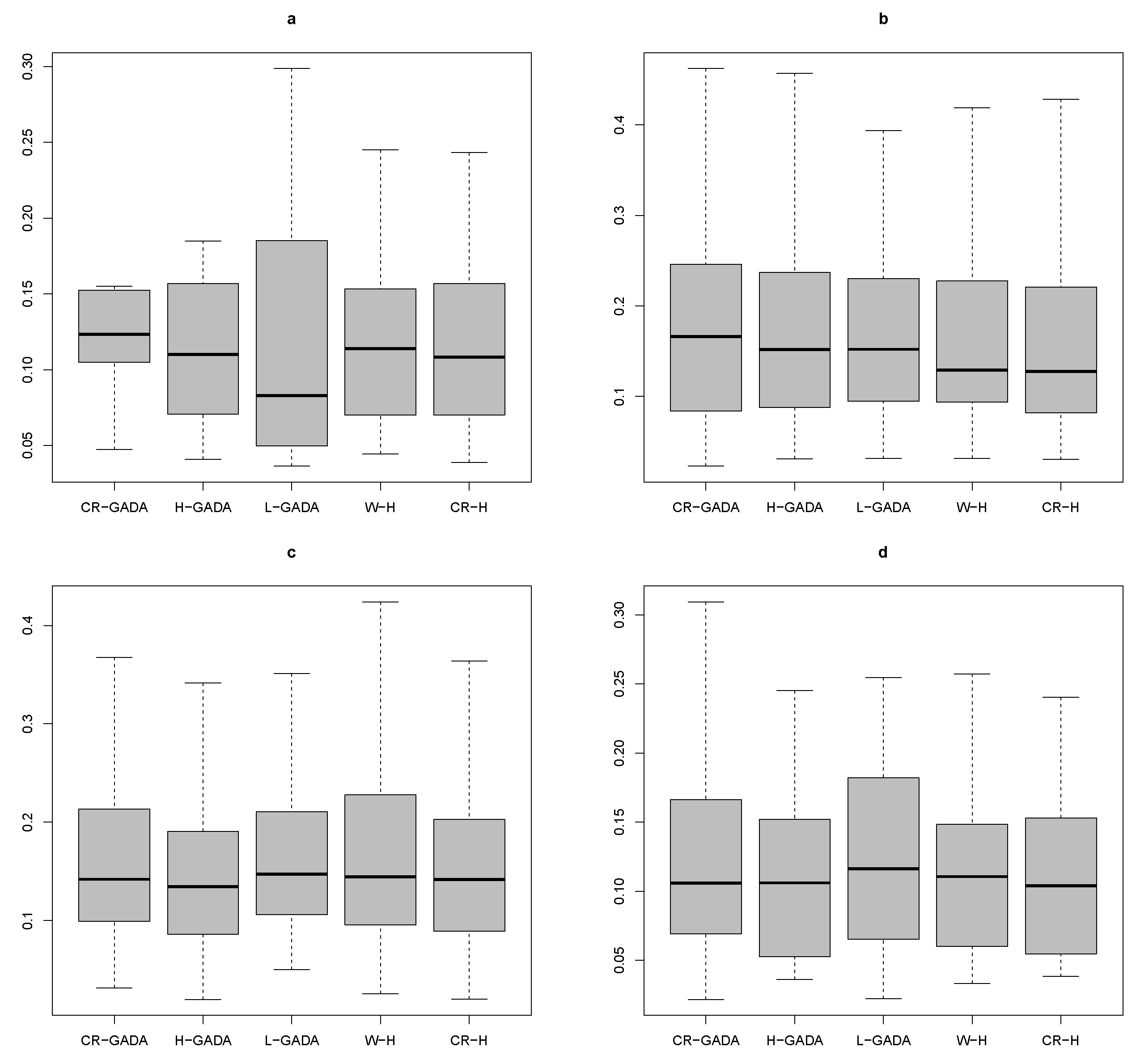
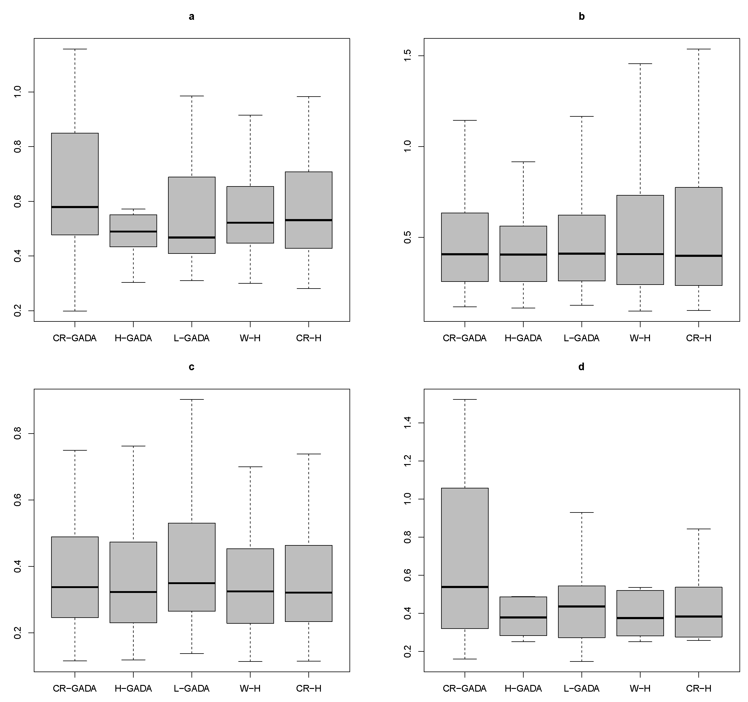
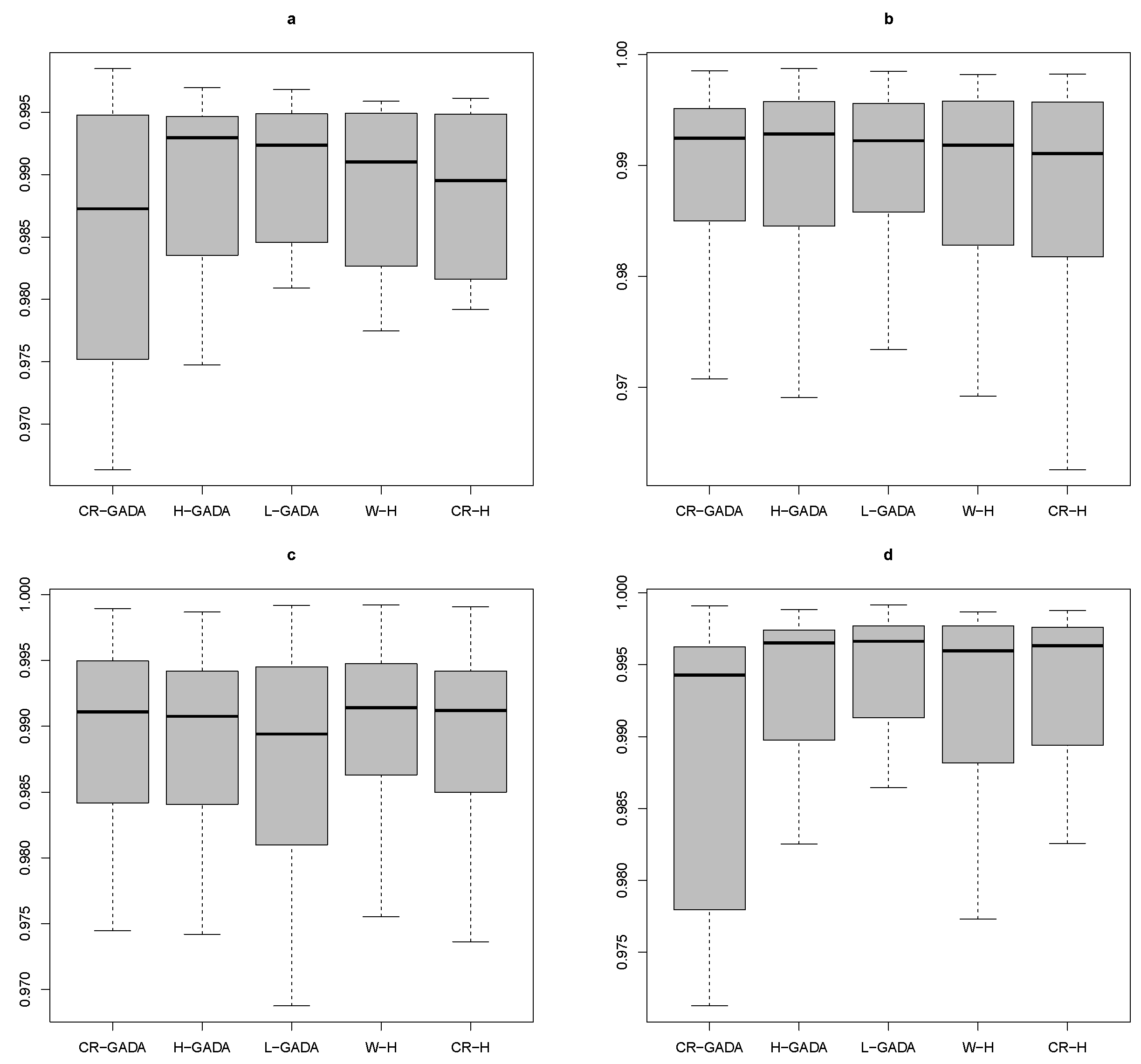
Applying the Kruskal-Wallis test to the four species studied (Pinus arizonica, Pinus engelmannii, Pinus strobiformis and Pinus teocote), we searched for possible differences between the CR-GADA, H-GADA, L-GADA and W-H models with respect to our proposed model (CR-H). Our results show that there are no significant differences in any of the parameters (MAPE, RMSE and R²) tested to compare the models, as the p-values for the K-W test were above 0.65 in all cases. In addition, the AIC values were also similar for each model (see

Table 4. Mean absolute percentage error (MAPE) and respective standard deviation results for each species and model considered.

Model	Pinus arizonica	Pinus engelmannii	Pinus strobiformis	Pinus teocote
CR-GADA	$0.13\pm 0.06$	$0.18\pm 0.11$	$0.19\pm 0.14$	$0.13\pm 0.09$
H-GADA	$0.13\pm 0.08$	$0.18\pm 0.11$	$0.17\pm 0.12$	$0.11\pm 0.07$
L-GADA	$0.11\pm 0.08$	$0.17\pm 0.11$	$0.20\pm 0.14$	$0.12\pm 0.07$
W-H	$0.13\pm 0.07$	$0.17\pm 0.11$	$0.18\pm 0.13$	$0.12\pm 0.07$
CR-H	$0.13\pm 0.07$	$0.17\pm 0.11$	$0.17\pm 0.12$	$0.11\pm 0.06$

,

Table 5. Root Mean Square Error (RMSE) and respective standard deviation results for each species and model of the study.

Model	Pinus arizonica	Pinus engelmannii	Pinus strobiformis	Pinus teocote
CR-GADA	$0.27\pm 0.18$	$0.19\pm 0.132$	$0.19\pm 0.12$	$0.25\pm 0.25$
H-GADA	$0.25\pm 0.19$	$0.19\pm 0.132$	$0.16\pm 0.13$	$0.19\pm 0.17$
L-GADA	$0.26\pm 0.19$	$0.19\pm 0.130$	$0.17\pm 0.12$	$0.19\pm 0.19$
W-H	$0.27\pm 0.20$	$0.21\pm 0.187$	$0.15\pm 0.11$	$0.19\pm 0.19$
CR-H	$0.27\pm 0.21$	$0.22\pm 0.197$	$0.16\pm 0.12$	$0.19\pm 0.19$

,

Table 6. R² and respective standard deviation results for each species and model in the study.

Model	Pinus arizonica	Pinus engelmannii	Pinus strobiformis	Pinus teocote
CR-GADA	$0.98\pm 0.02$	$0.99\pm 0.02$	$0.99\pm 0.01$	$0.99\pm 0.01$
H-GADA	$0.98\pm 0.03$	$0.99\pm 0.02$	$0.99\pm 0.01$	$0.99\pm 0.01$
L-GADA	$0.98\pm 0.03$	$0.99\pm 0.02$	$0.99\pm 0.01$	$0.99\pm 0.01$
W-H	$0.98\pm 0.03$	$0.99\pm 0.02$	$0.99\pm 0.01$	$0.99\pm 0.01$
CR-H	$0.98\pm 0.03$	$0.99\pm 0.02$	$0.99\pm 0.01$	$0.99\pm 0.01$

and

Table 7. AIC results for each species and model of the study.

Model	Pinus arizonica	Pinus engelmannii	Pinus strobiformis	Pinus teocote
CR-GADA	2559.62	15806.01	4158.34	2064.44
H-GADA	2528.21	14506.80	4159.03	1898.75
L-GADA	2526.19	14507.73	4163.67	1897.72
W-H	2525.34	14576.58	4164.76	1894.80
CR-H	2525.58	14590.79	4159.92	1895.04

and Figure 4, Figure 5 and Figure 6).

4. Discussion and Conclusions

The results show a strong negative association between the maximum yield of the growth parameters, given at the final dimension reached at the end of their respective growth period (${\theta }_1$) and the maximum specific growth rate (${\theta }_2$). In other words, the less value has the slope (current annual increment) in the inflexion point of the growth curve of the tree, the greater the final maximum yield. Additionally, ${\theta }_2$ depends on the actual environment and initial physiological state of the population/trees [28]. The accuracy of our GADA and H models (W-H and CR-H) was similar to the GADA models of other studies (e.g., [17,29,30,31]).

The main advantage of the widely used GADA site index models over ADA is that they can be polymorphic and have multiple asymptotes caused by more than one site-specific parameter to create functions of ${\chi }_0$ (i.e., one unobservable independent variable which describes site productivity, as a summary of management regimes, soil, climatic and ecological factors) [29,30]. This leads to more flexible dynamic models [31]. However, if these site-specific parameters are highly correlated to each other, as we have shown (Figure 2), these several parameters could be replaced by the single parameter easiest to estimate in the forest practice, making the model mathematically and economically more attractive due to the smaller number of parameters, which makes a complex multiparametric ${\chi }_0$ function obsolete, without compromising the fitting capability of the model Table 4, Table 5, Table 6 and Table 7 [22,26]. I.e., the main advantage of this novel CR-H model over GADA is the simplification described above by reducing the number of site-specific parameters to the only one most easily measurable site-specific parameter, while statistically maintaining the predictive quality of the model. Moreover, in contrast to the CR-GADA factor ${\chi }_0$, when ${\theta }_2$ is assumed to be site-specific [18], the CR-H has always a closed-form solution.

The study findings show that the model proposed in this study is accurate and feasible, at least for the population analyzed. This model can be classified as a hybrid, as we initially applied a variable substitution of the type ${\theta }_2=a/{\theta }_1$, to then assume that the parameter a is site-specific (ADA methodology). If the relationship shown by parameters ${\theta }_1$ and ${\theta }_2$ can also be reproduced in data sets for other organisms, this new model will greatly reduce the economical and computational effort invested in obtaining the model parameters.

Although the quality of the five growth models applied in the experiment was very similar from a statistical point of view, the proposed CR-H, like the W-H, is easy to apply, as it has only ${\theta }_1$ as a parameter, which is the maximum tree diameter or the final diameter of the tree at the end of its respective growth stage. This parameter can be easily obtained, by measuring just the dominant trees, especially in coniferous forests with irregular ages.

It would be interesting for a future study to test the same hypothesis with other species and other growth models, in order to determine whether the CR-H model performance is replicated. Furthermore, sufficiently high correlations of the site-specific parameters ${\theta }_1$, ${\theta }_2$ and ${\theta }_3$, and therefore, the accuracy of these simplified dynamic H models should be tested, when environmental changes and competition parameters are incorporated into the models that effectively perturb the growth of individuals.