
Terrestrial Water Storage Dynamics: Different Roles of Climate Variability, Vegetation Change, and Human Activities across Climate Zones in China

Abstract
:1. Introduction
2. Materials and Methods
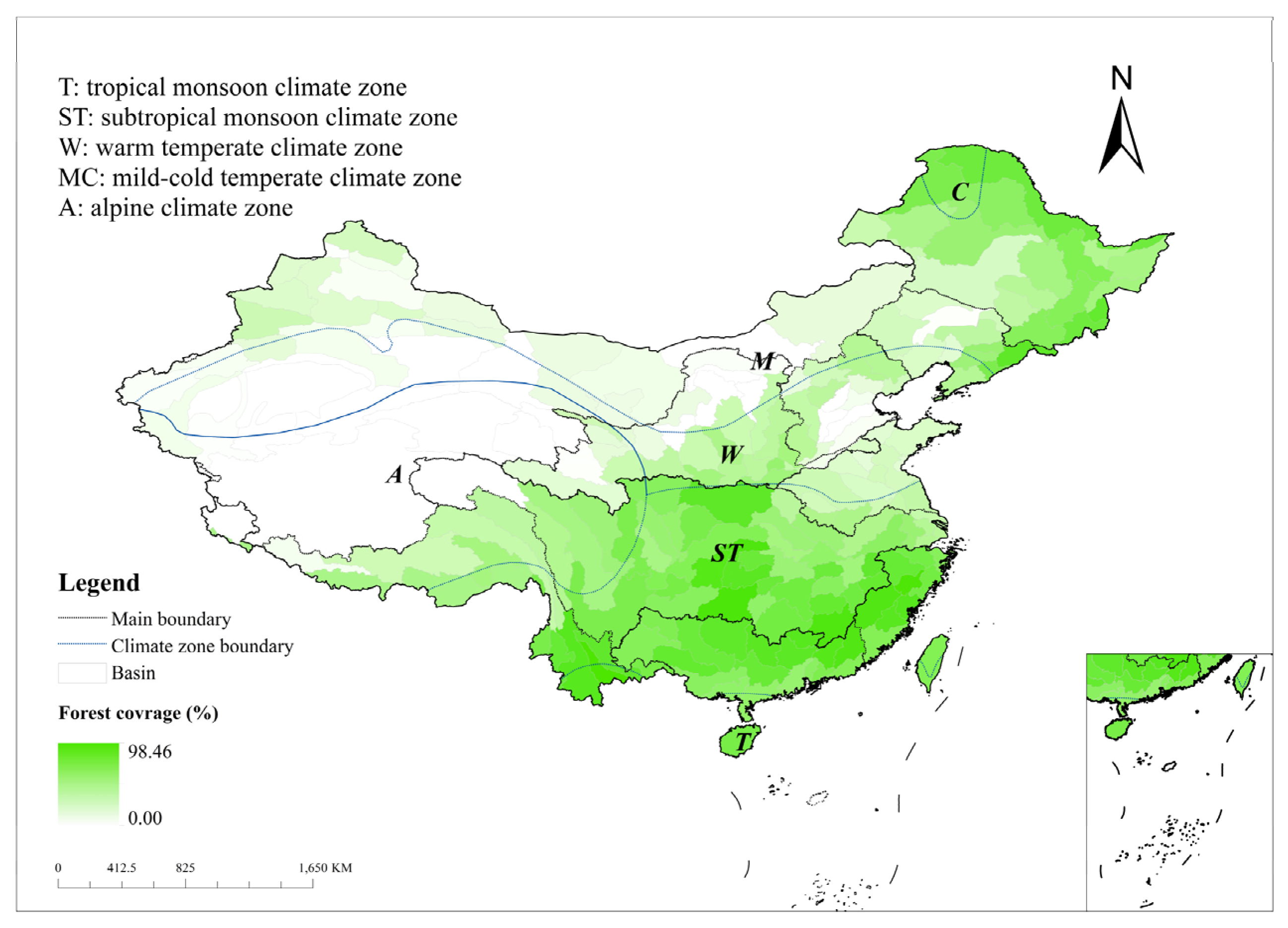
2.1. Study Area
2.2. Data
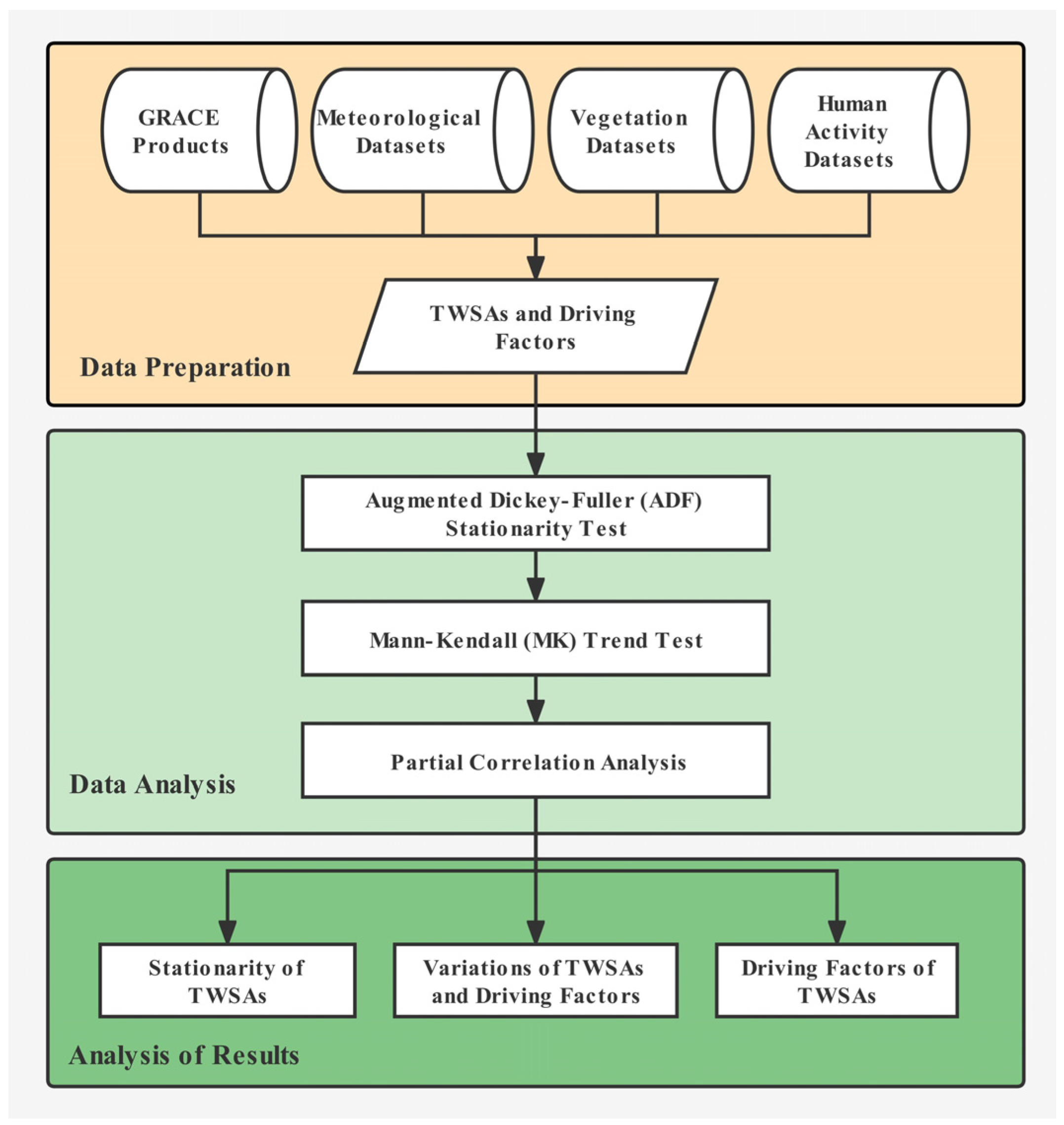
2.3. Methods
3. Results
3.1. TWSAs and Driving Factors: Trend and Stationarity
3.1.1. Trends and Stationarities of TWSAs
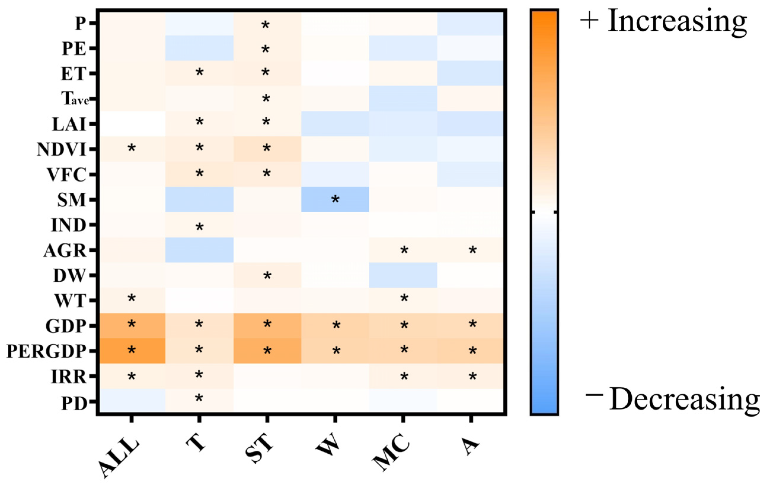
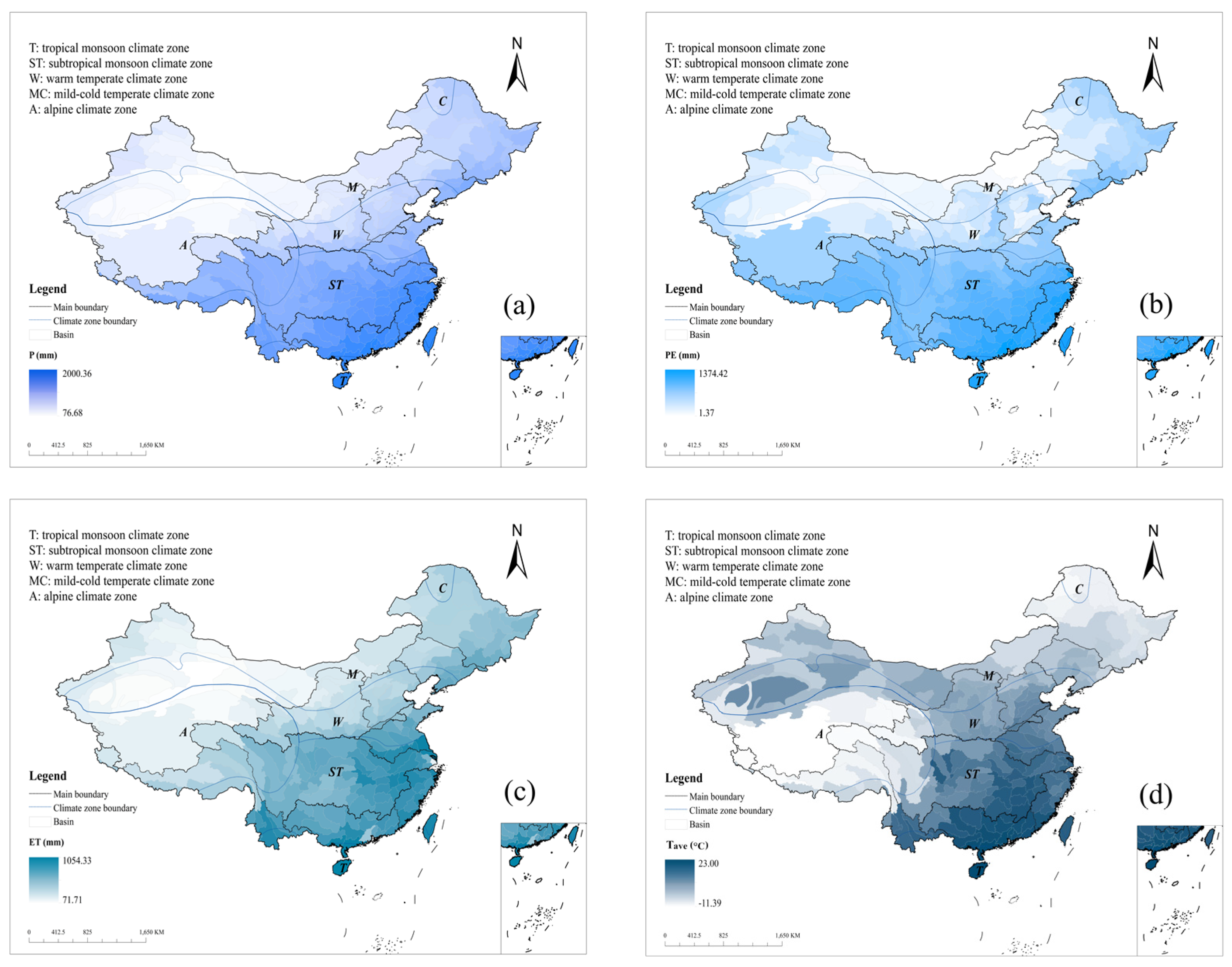
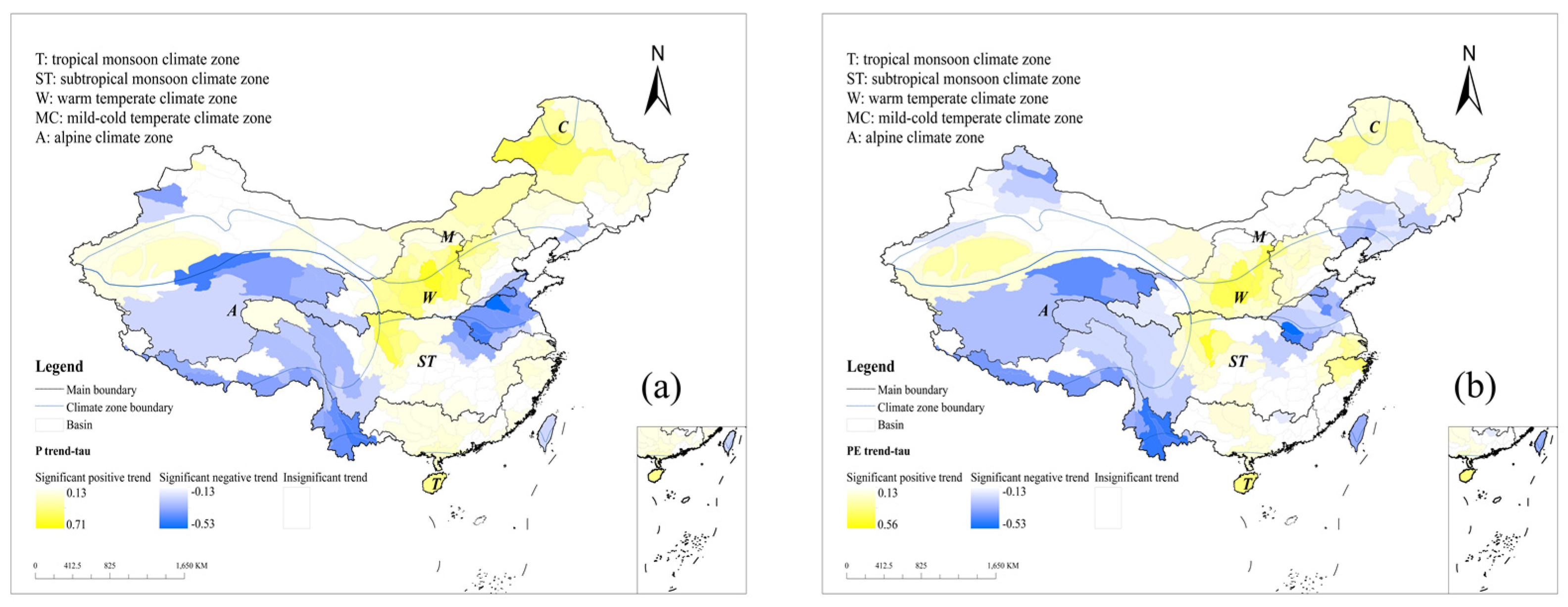
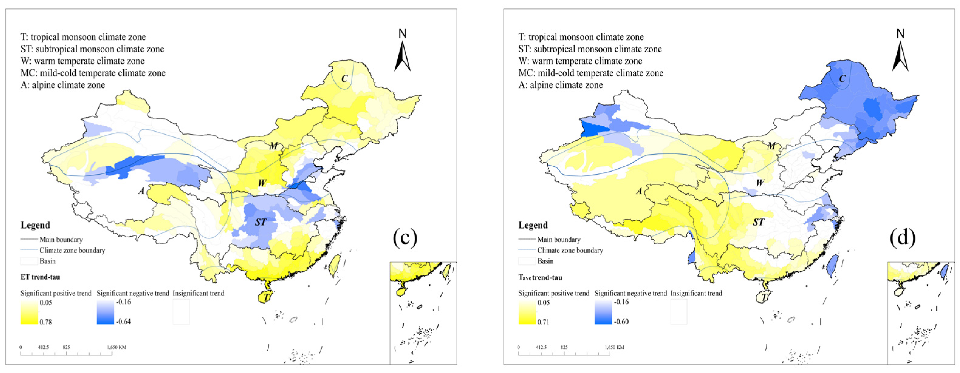
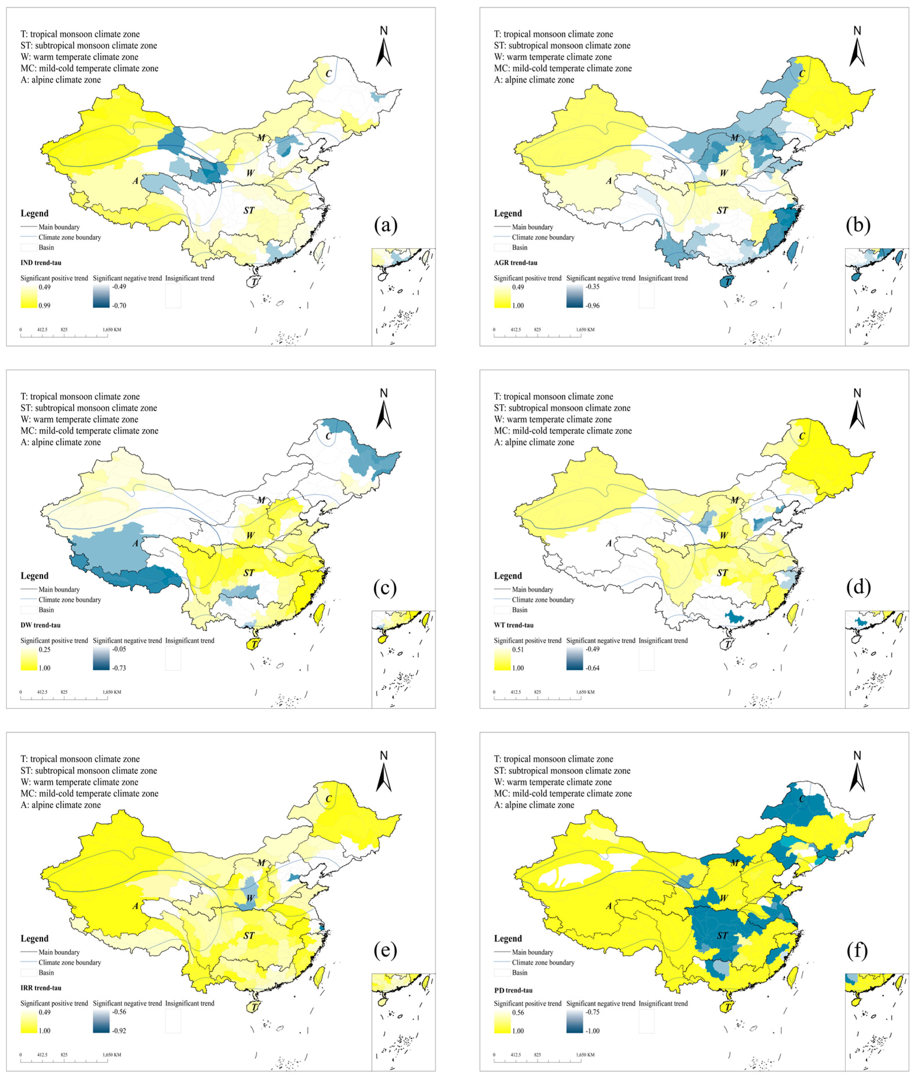
3.1.2. Trends of Driving Factors
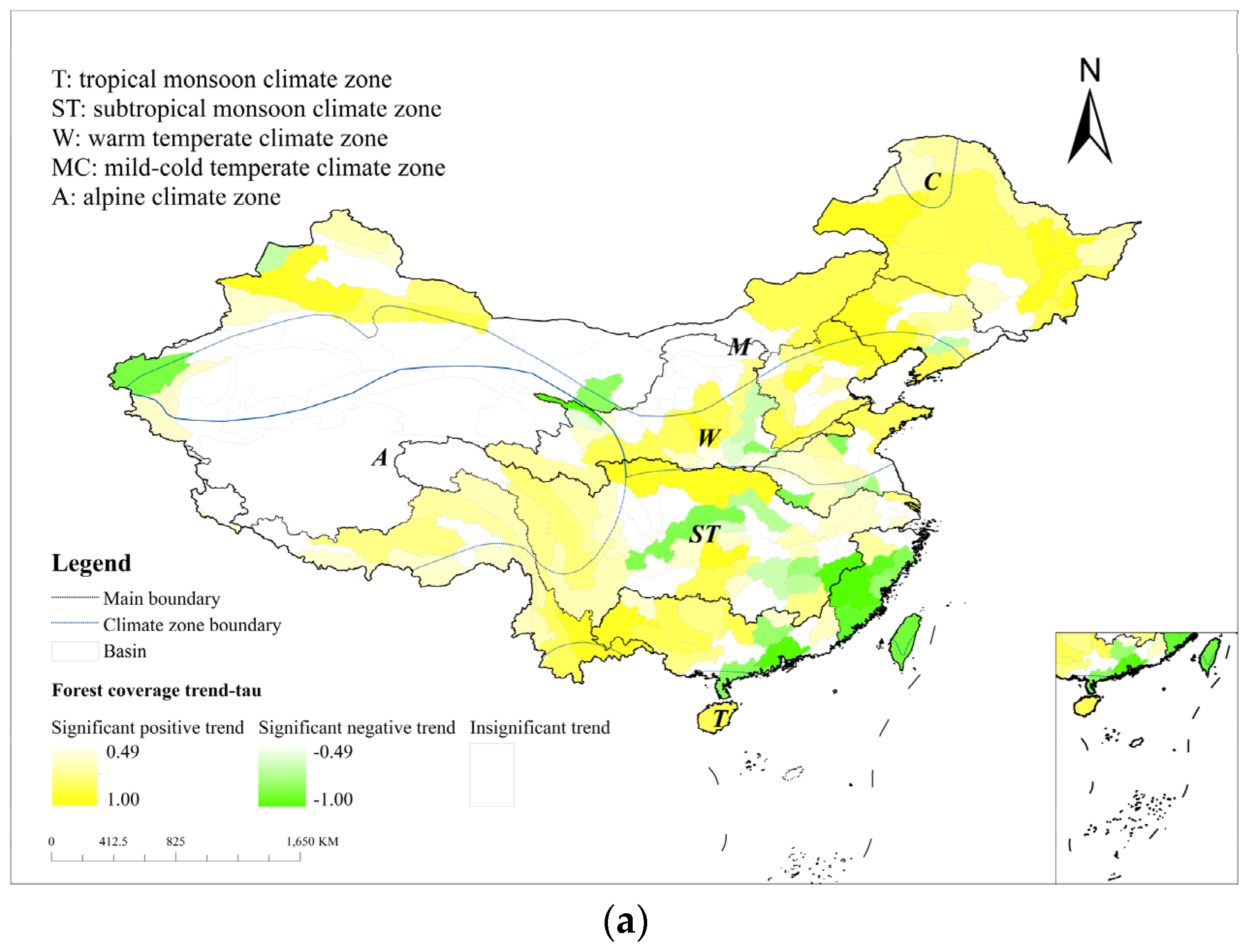
3.2. Spatial Variations of TWSAs
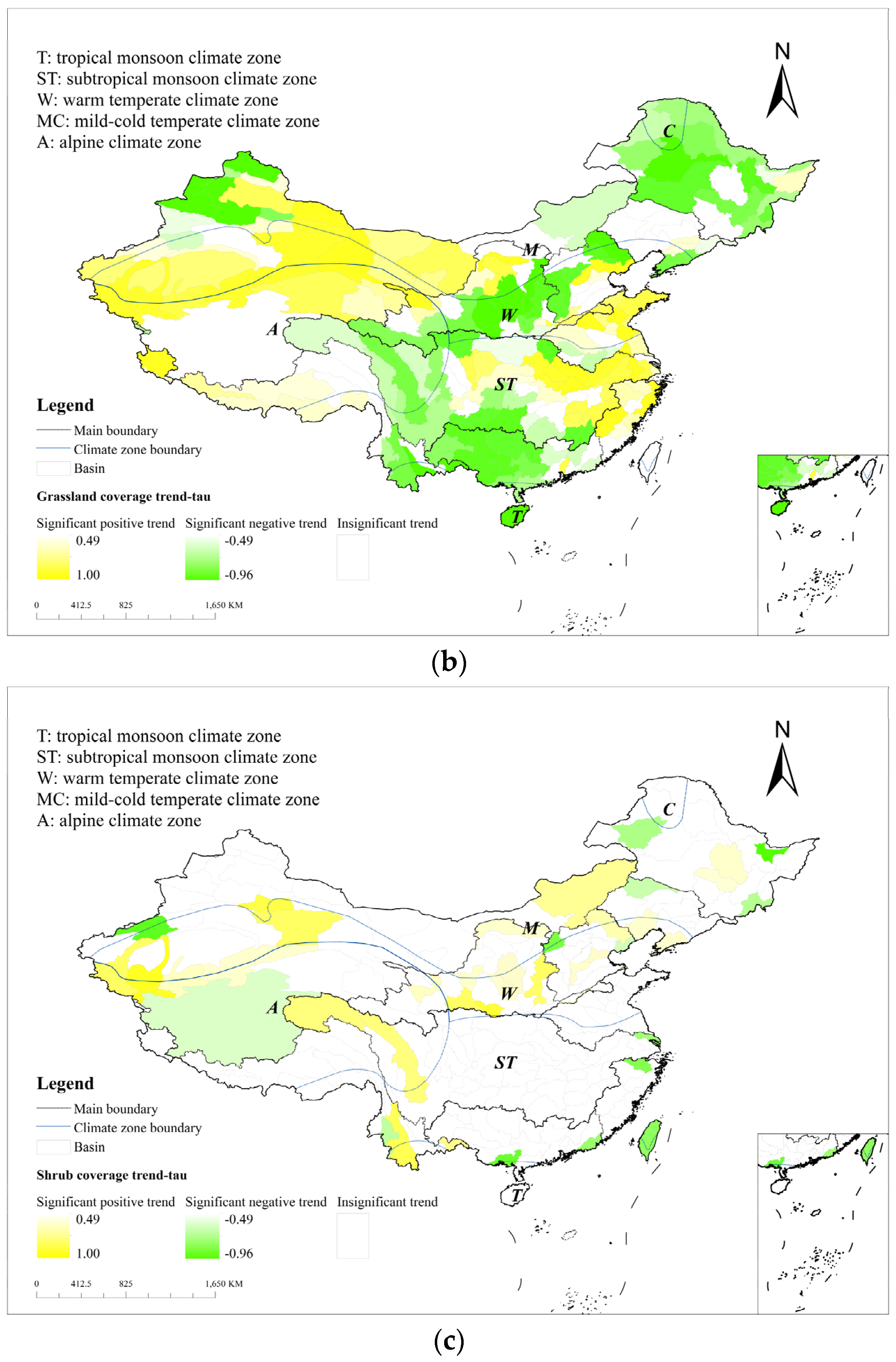
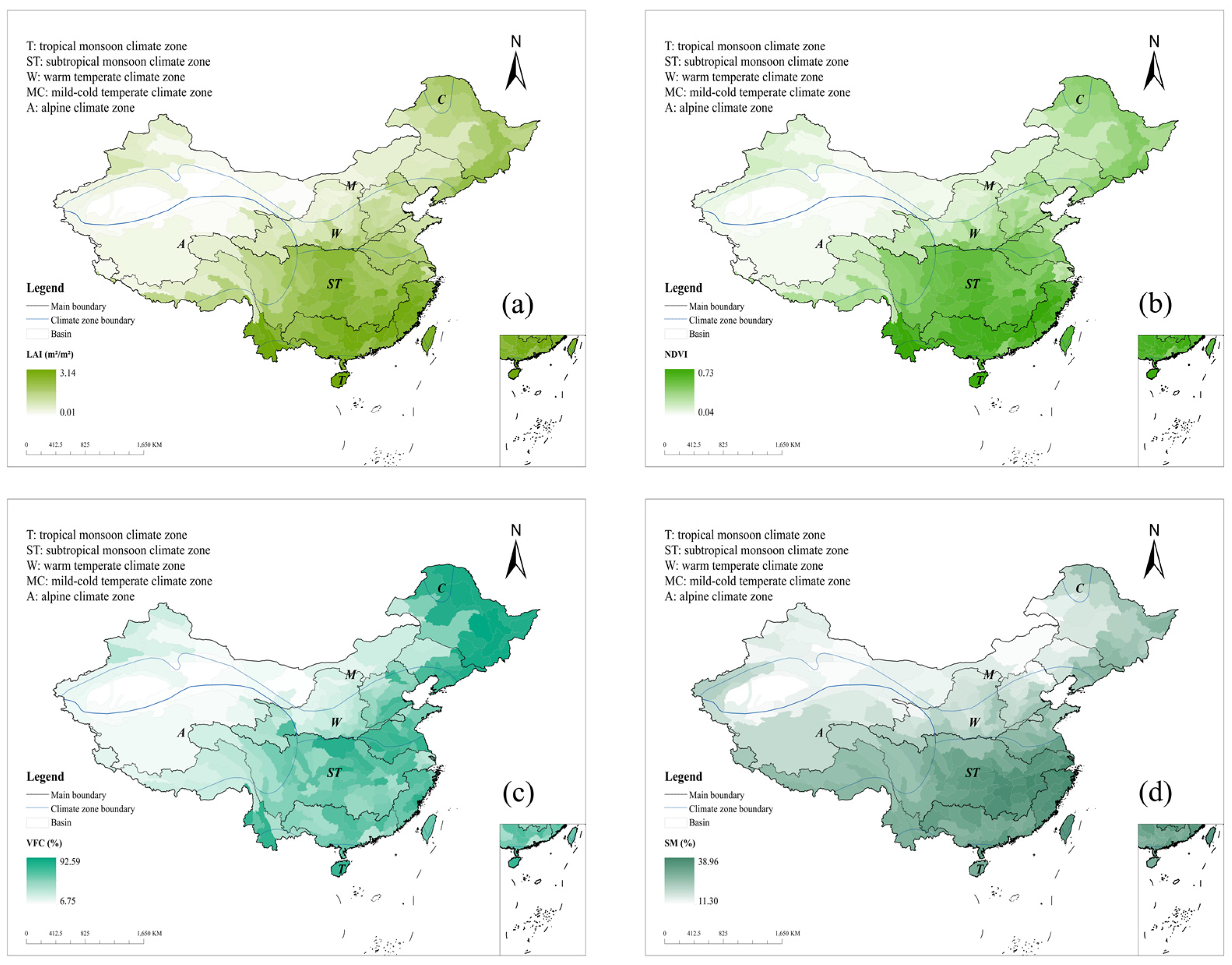
3.3. Spatial Variations of Vegetation Change
3.4. Key Driving Factors for TWSAs in Different Climate Zones
4. Discussion
4.1. The Dynamics of Terrestrial Water Storage and Their Driving Factors across Climate Zones
4.2. Limitations and Uncertainties
5. Conclusions
Author Contributions
Funding
Institutional Review Board Statement
Informed Consent Statement
Data Availability Statement
Acknowledgments
Conflicts of Interest
Abbreviations
| Terrestrial water storage | TWS |
| Terrestrial water storage anomalies | TWSAs |
| Gravity Recovery and Climate Experiment | GRACE |
| Mann-Kendall | MK |
| Augmented Dickey-Fuller | ADF |
| Forest coverage | FC |
| Shrub coverage | SC |
| Grassland coverage | GC |
| Tropical monsoon zones | T |
| Subtropical monsoon zones | ST |
| Warm temperate zones | W |
| Mild temperate zones | M |
| Cold temperate zones | C |
| Alpine climate zones | A |
| Mild-Cold temperate zone | MC |
Appendix A


Appendix B


| NO. | ID | Climate Zone | Area (km2) | P (mm) | Tave (°C) | TWS MK tau |
|---|---|---|---|---|---|---|
| 1 | A010100 | MC | 41,473.19 | 339.86 | 1.25 | 0.49 * |
| 2 | A010200 | MC | 58,611.51 | 437.43 | −0.66 | 0.45 * |
| 3 | A010300 | MC | 61,341.18 | 490.53 | −2.15 | 0.45 * |
| 4 | A020100 | MC | 69,452.51 | 566.96 | −0.13 | 0.42 * |
| 5 | A020200 | MC | 100,618.63 | 545.90 | 1.64 | 0.45 * |
| 6 | A020300 | MC | 138,267.04 | 520.10 | 4.21 | 0.42 * |
| 7 | A030100 | MC | 45,964.14 | 846.76 | 3.64 | 0.49 * |
| 8 | A030200 | MC | 33,667.01 | 688.09 | 4.91 | 0.31 |
| 9 | A040100 | MC | 32,730.16 | 652.25 | 4.18 | 0.27 |
| 10 | A040200 | MC | 64,548.34 | 648.47 | 2.99 | 0.38 |
| 11 | A040300 | MC | 41,242.49 | 700.78 | 2.43 | 0.42 |
| 12 | A040400 | MC | 44,987.73 | 675.08 | 1.82 | 0.49 * |
| 13 | A040500 | MC | 18,271.14 | 714.84 | 2.92 | 0.49 * |
| 14 | A050100 | MC | 123,785.80 | 620.06 | −0.65 | 0.42 |
| 15 | A060100 | MC | 24,845.07 | 679.86 | 2.79 | 0.56 * |
| 16 | A060200 | MC | 42,589.81 | 747.77 | 2.94 | 0.60 * |
| 17 | A070100 | MC | 11,441.55 | 691.30 | 2.44 | 0.60 * |
| 18 | A080100 | MC | 25,049.50 | 756.74 | 3.34 | 0.53 * |
| 19 | B010100 | W | 63,196.65 | 467.47 | 5.25 | 0.05 |
| 20 | B010200 | MC | 39,231.93 | 434.38 | 5.26 | 0.20 |
| 21 | B010300 | MC | 38,082.83 | 503.81 | 7.79 | 0.20 |
| 22 | B020100 | MC | 10,821.14 | 688.19 | 5.77 | 0.24 |
| 23 | B030100 | MC | 36,985.69 | 681.83 | 7.16 | 0.20 |
| 24 | B030200 | W | 14,168.27 | 690.43 | 8.72 | 0.27 |
| 25 | B040100 | W | 12,290.00 | 877.16 | 6.25 | 0.38 |
| 26 | B040200 | W | 16,747.98 | 875.84 | 6.65 | 0.42 |
| 27 | B050100 | MC | 24,471.30 | 982.81 | 3.72 | 0.53* |
| 28 | B050200 | W | 10,410.43 | 973.22 | 5.96 | 0.42 |
| 29 | B060100 | W | 26,227.84 | 856.18 | 7.91 | 0.24 |
| 30 | B060200 | W | 38,053.53 | 594.56 | 8.68 | 0.16 |
| 31 | C010100 | W | 45,043.11 | 530.77 | 6.49 | −0.27 |
| 32 | C010200 | W | 11,308.64 | 603.37 | 11.12 | −0.42 |
| 33 | C020100 | W | 22,293.76 | 546.10 | 8.43 | −0.56 * |
| 34 | C020200 | W | 17,729.95 | 445.14 | 6.22 | −0.85 * |
| 35 | C020300 | W | 28,154.55 | 477.38 | 6.32 | −0.78 * |
| 36 | C020400 | W | 16,277.47 | 541.11 | 12.20 | −0.64 * |
| 37 | C030100 | W | 18,829.10 | 495.42 | 9.46 | −0.82 * |
| 38 | C030200 | W | 12,962.85 | 518.92 | 13.11 | −0.78 * |
| 39 | C030300 | W | 13,998.49 | 525.19 | 13.17 | −0.75 * |
| 40 | C030400 | W | 31,242.82 | 522.33 | 9.23 | −0.89 * |
| 41 | C030500 | W | 15,424.85 | 558.94 | 14.16 | −0.89 * |
| 42 | C030600 | W | 26,510.46 | 582.60 | 10.40 | −0.82 * |
| 43 | C030700 | W | 9371.70 | 650.03 | 15.22 | −0.82 * |
| 44 | C030800 | W | 23,159.94 | 573.61 | 14.22 | −0.78 * |
| 45 | C040100 | W | 33,173.78 | 614.12 | 14.25 | −0.82 * |
| 46 | D010100 | A | 86,810.32 | 643.16 | −1.09 | 0.42 |
| 47 | D010200 | A | 45,624.64 | 510.67 | 0.96 | 0.31 |
| 48 | D020100 | A | 14,712.22 | 289.19 | −1.34 | −0.31 |
| 49 | D020200 | A | 16,408.75 | 350.02 | 3.51 | −0.31 |
| 50 | D020300 | A | 33,226.18 | 587.09 | 3.29 | −0.42 |
| 51 | D020400 | A | 26,522.28 | 407.34 | 4.21 | −0.38 |
| 52 | D030100 | A | 29,972.50 | 373.51 | 8.08 | −0.82 * |
| 53 | D030200 | W | 24,190.04 | 327.31 | 8.75 | −0.93 * |
| 54 | D030300 | MC | 31,760.93 | 238.31 | 9.84 | −0.96 * |
| 55 | D030400 | MC | 56,017.33 | 298.32 | 6.45 | −0.89 * |
| 56 | D030500 | MC | 21,255.23 | 301.16 | 8.44 | −0.89 * |
| 57 | D040100 | W | 39,045.65 | 452.61 | 8.48 | −0.93 * |
| 58 | D040200 | W | 23,669.62 | 394.27 | 8.71 | −0.93 * |
| 59 | D040300 | W | 48,479.81 | 420.97 | 10.01 | −1.00 * |
| 60 | D050100 | W | 40,106.59 | 528.62 | 9.07 | −0.89 * |
| 61 | D050200 | W | 24,996.79 | 504.66 | 9.67 | −0.82 * |
| 62 | D050300 | W | 43,799.44 | 486.02 | 9.49 | −0.82 * |
| 63 | D050400 | A | 31,078.78 | 554.87 | 7.40 | −0.75 * |
| 64 | D050500 | ST | 17,632.94 | 655.79 | 11.36 | −0.75 * |
| 65 | D050600 | ST | 18,413.12 | 664.77 | 12.52 | −0.78 * |
| 66 | D050700 | W | 16,102.14 | 644.92 | 12.63 | −0.75 * |
| 67 | D060100 | W | 6009.98 | 666.76 | 12.03 | −0.78 * |
| 68 | D060200 | W | 13,762.79 | 613.06 | 10.18 | −0.82 * |
| 69 | D060300 | ST | 18,918.75 | 711.46 | 12.22 | −0.71 * |
| 70 | D060400 | W | 3327.59 | 678.51 | 14.15 | −0.82 * |
| 71 | D070100 | W | 7570.86 | 676.30 | 15.32 | −0.82 * |
| 72 | D070200 | W | 11,520.84 | 699.17 | 13.12 | −0.82 * |
| 73 | D070300 | W | 4523.98 | 691.39 | 15.04 | −0.75 * |
| 74 | D080100 | MC | 43,524.95 | 285.24 | 8.71 | −0.93 * |
| 75 | E010100 | ST | 16,198.71 | 942.52 | 16.11 | −0.42 |
| 76 | E010200 | ST | 14,804.98 | 1028.58 | 16.03 | 0.05 |
| 77 | E020100 | ST | 67,661.97 | 828.15 | 15.47 | −0.78 * |
| 78 | E020200 | ST | 25,178.55 | 1122.53 | 15.77 | 0.05 |
| 79 | E020300 | ST | 31,742.58 | 889.09 | 15.50 | −0.82 * |
| 80 | E020400 | ST | 8401.70 | 1068.95 | 15.96 | −0.45 |
| 81 | E030100 | ST | 7851.87 | 1100.24 | 15.72 | −0.53 * |
| 82 | E030200 | ST | 25,017.33 | 1131.08 | 15.18 | −0.56 * |
| 83 | E040100 | W | 10,036.48 | 742.36 | 14.35 | −0.82 * |
| 84 | E040200 | W | 22,433.73 | 738.29 | 15.12 | −0.82 * |
| 85 | E040300 | W | 9751.93 | 838.77 | 14.65 | −0.82 * |
| 86 | E040400 | ST | 33,578.17 | 867.59 | 13.71 | −0.85 * |
| 87 | E040500 | W | 4179.98 | 843.47 | 13.33 | −0.82 * |
| 88 | E050100 | W | 14,550.42 | 680.76 | 13.43 | −0.82 * |
| 89 | E050200 | W | 48,336.09 | 744.74 | 12.52 | −0.53 * |
| 90 | F010100 | A | 146,040.82 | 408.21 | −3.91 | 0.60 * |
| 91 | F010200 | ST | 74,779.04 | 949.22 | 1.51 | −0.82 * |
| 92 | F020100 | ST | 12,8821.94 | 925.24 | 2.98 | −0.56 * |
| 93 | F020200 | ST | 12,8766.38 | 943.55 | 10.92 | −0.49 * |
| 94 | F030100 | ST | 77,155.92 | 937.02 | 2.90 | −0.27 |
| 95 | F030200 | ST | 58,696.32 | 935.55 | 9.22 | 0.05 |
| 96 | F030300 | ST | 27,132.36 | 955.36 | 17.28 | 0.49 * |
| 97 | F040100 | ST | 60,368.63 | 752.94 | 7.95 | −0.38 |
| 98 | F040200 | ST | 35,868.57 | 934.51 | 14.67 | 0.42 |
| 99 | F040300 | ST | 39,064.36 | 1017.61 | 15.51 | 0.42 |
| 100 | F040400 | ST | 23,800.93 | 966.02 | 16.77 | 0.38 |
| 101 | F050100 | ST | 51,083.17 | 1018.07 | 13.72 | 0.56 * |
| 102 | F050200 | ST | 36,997.82 | 1071.45 | 13.99 | 0.75 * |
| 103 | F060100 | ST | 19,092.87 | 940.97 | 14.56 | 0.49 * |
| 104 | F060200 | ST | 80,857.98 | 1054.45 | 15.53 | 0.71 * |
| 105 | F070100 | ST | 18,158.75 | 1211.08 | 14.69 | 0.75 * |
| 106 | F070200 | ST | 54,417.17 | 1180.79 | 15.36 | 0.78 * |
| 107 | F070300 | ST | 35,395.90 | 1200.50 | 15.33 | 0.78 * |
| 108 | F070400 | ST | 16,515.17 | 1272.79 | 16.04 | 0.82 * |
| 109 | F070500 | ST | 11,910.24 | 1277.88 | 15.74 | 0.78 * |
| 110 | F070600 | ST | 54,040.31 | 1360.81 | 17.15 | 0.75 * |
| 111 | F070700 | ST | 41,728.33 | 1343.38 | 17.48 | 0.78 * |
| 112 | F070800 | ST | 32,260.72 | 1262.03 | 17.29 | 0.75 * |
| 113 | F080100 | ST | 94,742.01 | 854.58 | 11.43 | −0.31 |
| 114 | F080200 | ST | 24,414.02 | 887.86 | 15.22 | −0.27 |
| 115 | F080300 | ST | 37,232.54 | 1059.64 | 15.33 | 0.53 * |
| 116 | F090100 | ST | 14,854.61 | 1432.96 | 16.08 | 0.75 * |
| 117 | F090200 | ST | 40,910.15 | 1547.86 | 17.74 | 0.67 * |
| 118 | F090300 | ST | 23,643.46 | 1472.95 | 17.60 | 0.71 * |
| 119 | F090400 | ST | 19,821.07 | 1468.32 | 17.65 | 0.78 * |
| 120 | F090500 | ST | 16,201.79 | 1601.23 | 17.60 | 0.67 * |
| 121 | F090600 | ST | 15,990.92 | 1688.19 | 16.99 | 0.64 * |
| 122 | F090700 | ST | 14,806.03 | 1574.38 | 16.99 | 0.67 * |
| 123 | F090800 | ST | 20,302.84 | 1497.02 | 17.66 | 0.75 * |
| 124 | F100100 | ST | 17,770.44 | 1154.60 | 12.72 | 0.78 * |
| 125 | F100200 | ST | 21,790.17 | 1142.38 | 16.20 | 0.71 * |
| 126 | F100300 | ST | 34,251.96 | 1158.87 | 16.54 | 0.49 * |
| 127 | F100400 | ST | 23,017.81 | 1325.82 | 16.93 | 0.71 * |
| 128 | F110100 | ST | 43,495.11 | 1236.87 | 16.18 | 0.20 |
| 129 | F110200 | ST | 35,552.60 | 1363.98 | 15.74 | 0.35 |
| 130 | F110300 | ST | 13,876.48 | 1306.54 | 15.89 | −0.35 |
| 131 | F120100 | ST | 17,820.64 | 1387.83 | 15.85 | 0.05 |
| 132 | F120200 | ST | 8436.70 | 1348.46 | 16.07 | −0.20 |
| 133 | F120300 | ST | 7742.61 | 1512.98 | 16.48 | 0.20 |
| 134 | F120400 | ST | 4757.13 | 1420.43 | 16.36 | −0.09 |
| 135 | G010100 | ST | 33,071.13 | 1696.34 | 15.77 | 0.56 * |
| 136 | G010200 | ST | 18,726.80 | 1661.86 | 15.61 | 0.35 |
| 137 | G020100 | ST | 10812.38 | 1722.91 | 16.31 | 0.27 |
| 138 | G020200 | ST | 1365.86 | 1782.27 | 0.00 | 0.36 |
| 139 | G030100 | ST | 15,229.00 | 1841.64 | 15.04 | 0.45 |
| 140 | G030200 | ST | 20,192.22 | 1865.49 | 15.53 | 0.42 |
| 141 | G040100 | ST | 17,009.52 | 1799.32 | 15.80 | 0.45 |
| 142 | G050100 | ST | 43,534.09 | 1676.38 | 16.65 | 0.60 * |
| 143 | G050200 | ST | 19,234.41 | 1730.08 | 16.85 | 0.53 * |
| 144 | G060100 | ST | 35,963.54 | 1693.45 | 18.26 | 0.60 * |
| 145 | G070100 | T | 38,877.74 | 1954.36 | 17.13 | 0.53 * |
| 146 | H010100 | T | 57,507.93 | 1028.04 | 15.03 | 0.05 |
| 147 | H010200 | ST | 26,572.96 | 1031.86 | 14.45 | 0.16 |
| 148 | H020100 | ST | 54,832.13 | 1280.75 | 18.08 | 0.56 * |
| 149 | H020200 | ST | 58,769.39 | 1300.93 | 17.29 | 0.60 * |
| 150 | H030100 | ST | 39,411.43 | 1281.92 | 17.29 | 0.53 * |
| 151 | H030200 | ST | 38,725.63 | 1570.26 | 19.11 | 0.71 * |
| 152 | H040100 | ST | 30,395.15 | 1508.51 | 18.60 | 0.67 * |
| 153 | H040200 | ST | 36,462.52 | 1731.22 | 20.60 | 0.67 * |
| 154 | H050100 | ST | 17,729.86 | 1529.82 | 17.79 | 0.75 * |
| 155 | H050200 | ST | 29,770.64 | 1692.95 | 19.16 | 0.75 * |
| 156 | H060100 | ST | 19,340.65 | 1724.52 | 19.16 | 0.67 * |
| 157 | H060200 | ST | 9089.74 | 1889.35 | 20.97 | 0.67 * |
| 158 | H070100 | ST | 7689.55 | 1955.68 | 20.74 | 0.71 * |
| 159 | H070200 | ST | 1124.95 | 1965.12 | 21.34 | 0.71 * |
| 160 | H070300 | ST | 19,514.04 | 1974.55 | 21.94 | 0.71 * |
| 161 | H070400 | ST | 24.89 | 1823.90 | 20.39 | 0.49 |
| 162 | H080100 | ST | 29,405.44 | 1673.25 | 18.84 | 0.64 * |
| 163 | H080200 | ST | 17,691.43 | 1736.14 | 20.52 | 0.67 * |
| 164 | H090100 | T | 34,093.06 | 1850.01 | 22.40 | 0.60 * |
| 165 | H090200 | T | 22,151.88 | 1770.85 | 21.67 | 0.60 * |
| 166 | H100100 | T | 34,122.92 | 2000.36 | 23.00 | 0.24 |
| 167 | H100200 | T | 46.77 | 1576.70 | 19.87 | 0.23 |
| 168 | J010100 | T | 23,648.34 | 1153.04 | 16.73 | 0.20 |
| 169 | J010200 | T | 36,858.42 | 1038.22 | 15.97 | −0.13 |
| 170 | J010300 | T | 15,475.56 | 1199.31 | 16.32 | 0.38 |
| 171 | J020100 | ST | 92,175.82 | 867.20 | 0.08 | −0.82 * |
| 172 | J020200 | T | 74,639.37 | 1209.03 | 16.20 | 0.13 |
| 173 | J030100 | ST | 109,419.77 | 856.71 | −1.04 | −0.82 * |
| 174 | J030200 | T | 24,578.61 | 1121.37 | 15.96 | −0.38 |
| 175 | J030300 | ST | 21,843.12 | 1224.27 | 12.50 | −0.53 * |
| 176 | J040100 | A | 57,856.28 | 677.61 | −4.39 | −0.85 * |
| 177 | J040200 | A | 148,406.72 | 825.84 | −0.95 | −0.93 * |
| 178 | J040300 | ST | 52,439.60 | 968.40 | 2.38 | −0.93 * |
| 179 | J050100 | ST | 151,638.00 | 1026.57 | 3.72 | −0.89 * |
| 180 | J060100 | A | 5622.61 | 238.17 | −11.39 | −0.49 * |
| 181 | J060200 | A | 59,445.04 | 465.36 | −4.96 | −0.89 * |
| 182 | K010100 | MC | 215,394.29 | 314.78 | 3.10 | 0.20 |
| 183 | K010200 | MC | 99,453.54 | 269.77 | 5.88 | −0.82 * |
| 184 | K020100 | A | 41,726.79 | 209.92 | 7.18 | −0.75 * |
| 185 | K020200 | A | 152,430.90 | 131.02 | 7.37 | −0.60 * |
| 186 | K020300 | A | 126,307.25 | 107.79 | 4.92 | −0.49 * |
| 187 | K020400 | W | 151,286.51 | 148.84 | 9.34 | −0.78 * |
| 188 | K030100 | A | 47,500.93 | 247.78 | −1.46 | 0.20 |
| 189 | K040100 | A | 78,565.45 | 216.56 | −1.46 | 0.67 * |
| 190 | K040200 | A | 202,154.52 | 118.15 | −0.17 | 0.82 * |
| 191 | K050100 | MC | 57,673.63 | 113.55 | 6.15 | −0.75 * |
| 192 | K050200 | W | 41,518.80 | 95.16 | 8.86 | −0.85 * |
| 193 | K050300 | W | 37,853.56 | 127.26 | 7.56 | −0.96 * |
| 194 | K060100 | MC | 50,693.78 | 276.03 | 1.81 | −0.16 |
| 195 | K060200 | MC | 26,241.70 | 215.73 | 4.42 | −0.38 |
| 196 | K060300 | MC | 8033.20 | 361.15 | 3.90 | −0.13 |
| 197 | K070100 | MC | 22,241.47 | 314.94 | 4.98 | −0.45 |
| 198 | K070200 | MC | 61,879.15 | 316.68 | 2.24 | −0.75 * |
| 199 | K080100 | MC | 88,652.18 | 208.83 | 8.03 | −0.64 * |
| 200 | K090100 | MC | 18,346.21 | 146.53 | 5.58 | −0.85 * |
| 201 | K090200 | MC | 85,909.97 | 243.12 | 4.99 | −0.75 * |
| 202 | K090300 | MC | 53,560.57 | 338.34 | 6.64 | −0.75 * |
| 203 | K100100 | A | 88,788.54 | 164.03 | 2.03 | −0.31 |
| 204 | K100200 | A | 98,125.46 | 255.45 | 1.77 | −0.49 * |
| 205 | K100300 | A | 87,948.13 | 298.22 | 3.96 | −0.49 * |
| 206 | K100400 | W | 54,636.34 | 262.86 | 6.65 | −0.60 * |
| 207 | K100500 | W | 41,588.46 | 196.08 | 6.65 | −0.75 * |
| 208 | K100600 | W | 111,173.19 | 119.92 | 4.58 | −0.89 * |
| 209 | K110100 | A | 73,358.80 | 107.87 | 7.36 | 0.02 |
| 210 | K110200 | A | 137,705.99 | 77.12 | 6.90 | 0.35 |
| 211 | K120100 | W | 33,832.29 | 122.80 | 5.39 | −0.85 * |
| 212 | K130100 | W | 234,953.07 | 110.99 | 13.63 | −0.64 * |
| 213 | K130200 | A | 134,052.61 | 74.68 | 11.06 | −0.75 * |
| 214 | K140100 | A | 791,638.02 | 277.51 | −5.13 | −0.47 * |
References
- Rodell, M.; Famiglietti, J.S. An analysis of terrestrial water storage variations in Illinois with implications for the Gravity Recovery and Climate Experiment (GRACE). Water Resour. Res. 2001, 37, 1327–1339. [Google Scholar] [CrossRef]
- Deng, H.J.; Pepin, N.C.; Liu, Q.; Chen, Y.N. Understanding the spatial differences in terrestrial water storage variations in the Tibetan Plateau from 2002 to 2016. Clim. Chang. 2018, 151, 379–393. [Google Scholar] [CrossRef]
- Kang, Z.; Nagel, P.; Pastor, R. Precise orbit determination for GRACE. Int. Space Geo. Syst. Sat. Dyn. 2003, 31, 1875–1881. [Google Scholar] [CrossRef]
- Gupta, D.; Dhanya, C.T. The potential of GRACE in assessing the flood potential of Peninsular Indian River basins. Int. J. Remote Sens. 2020, 41, 9007–9036. [Google Scholar] [CrossRef]
- Sinha, D.; Syed, T.H.; Famiglietti, J.S.; Reager, J.T.; Thomas, R.C. Characterizing Drought in India Using GRACE Observations of Terrestrial Water Storage Deficit. J. Hydrometeorol. 2017, 18, 381–396. [Google Scholar] [CrossRef]
- Seyoum, W.M.; Milewski, A.M. Improved methods for estimating local terrestrial water dynamics from GRACE in the Northern High Plains. Adv. Water Resour. 2017, 110, 279–290. [Google Scholar] [CrossRef]
- Yang, P.; Chen, Y.N. An analysis of terrestrial water storage variations from GRACE and GLDAS: The Tianshan Mountains and its adjacent areas, central Asia. Quatern. Int. 2015, 358, 106–112. [Google Scholar] [CrossRef]
- Dankwa, S.; Zheng, W.F.; Gao, B.; Li, X.L. Terrestrial Water Storage (TWS) Patterns Monitoring in the Amazon Basin Using Grace Observed: Its Trends and Characteristics. In Proceedings of the 2018 IEEE International Geoscience and Remote Sensing Symposium (IGARSS), Valencia, Spain, 22–27 July 2018; pp. 768–771. [Google Scholar] [CrossRef]
- Hu, Z.Y.; Zhang, Z.Z.; Sang, Y.F.; Qian, J.; Feng, W.; Chen, X.; Zhou, Q.M. Temporal and spatial variations in the terrestrial water storage across Central Asia based on multiple satellite datasets and global hydrological models. J. Hydrol. 2021, 596, 126013. [Google Scholar] [CrossRef]
- Wang, H.S.; Jia, L.L.; Steffen, H.; Wu, P.; Jiang, L.M.; Hsu, H.T.; Xiang, L.W.; Wang, Z.Y.; Hu, B. Increased water storage in North America and Scandinavia from GRACE gravity data. Nat. Geosci. 2013, 6, 38–42. [Google Scholar] [CrossRef]
- Pokhrel, Y.N.; Koirala, S.; Yeh, P.J.F.; Hanasaki, N.; Longuevergne, L.; Kanae, S.; Oki, T. Incorporation of groundwater pumping in a global Land Surface Model with the representation of human impacts. Water Resour. Res. 2015, 51, 78–96. [Google Scholar] [CrossRef]
- Famiglietti, J.S.; Lo, M.; Ho, S.L.; Bethune, J.; Anderson, K.J.; Syed, T.H.; Swenson, S.C.; de Linage, C.R.; Rodell, M. Satellites measure recent rates of groundwater depletion in California’s Central Valley. Geophys. Res. Lett. 2011, 38, L03403. [Google Scholar] [CrossRef]
- Humphrey, V.; Gudmundsson, L.; Seneviratne, S.I. Assessing Global Water Storage Variability from GRACE: Trends, Seasonal Cycle, Subseasonal Anomalies and Extremes. Surv. Geophys. 2016, 37, 357–395. [Google Scholar] [CrossRef]
- Hilker, T.; Lyapustin, A.I.; Tucker, C.J.; Hall, F.G.; Myneni, R.B.; Wang, Y.J.; Bi, J.; de Moura, Y.M.; Sellers, P.J. Vegetation dynamics and rainfall sensitivity of the Amazon. Proc. Natl. Acad. Sci. USA 2014, 111, 16041–16046. [Google Scholar] [CrossRef]
- Tobella, A.B.; Reese, H.; Almaw, A.; Bayala, J.; Malmer, A.; Laudon, H.; Ilstedt, U. The effect of trees on preferential flow and soil infiltrability in an agroforestry parkland in semiarid Burkina Faso. Water Resour. Res. 2014, 50, 3342–3354. [Google Scholar] [CrossRef]
- Taylor, R.G.; Scanlon, B.; Döll, P.; Rodell, M.; Van Beek, R.; Wada, Y.; Longuevergne, L.; Leblanc, M.; Famiglietti, J.S.; Edmunds, M.; et al. Ground water and climate change. Nat. Clim. Chang. 2013, 3, 322–329. [Google Scholar] [CrossRef]
- Rodell, M.; Famiglietti, J.S.; Wiese, D.N.; Reager, J.T.; Beaudoing, H.K.; Landerer, F.W.; Lo, M.H. Emerging trends in global freshwater availability. Nature 2019, 565, E7. [Google Scholar] [CrossRef]
- Frappart, F.; Papa, F.; da Silva, J.S.; Ramillien, G.; Prigent, C.; Seyler, F.; Calmant, S. Surface freshwater storage and dynamics in the Amazon basin during the 2005 exceptional drought. Environ. Res. Lett. 2012, 7, 044010. [Google Scholar] [CrossRef]
- Kuo, Y.N.; Lo, M.H.; Liang, Y.C.; Tseng, Y.H.; Hsu, C.W. Terrestrial Water Storage Anomalies Emphasize Interannual Variations in Global Mean Sea Level During 1997–1998 and 2015–2016 El Nino Events. Geophys. Res. Lett. 2021, 48, e2021GL094104. [Google Scholar] [CrossRef]
- Nie, N.; Zhang, W.C.; Guo, H.D.; Ishwaran, N. 2010–2012 drought and flood events in the Amazon Basin inferred by GRACE satellite observations. J. Appl. Remote Sens. 2015, 9, 096023. [Google Scholar] [CrossRef]
- Zhang, G.Q.; Yao, T.D.; Shum, C.K.; Yi, S.; Yang, K.; Xie, H.J.; Feng, W.; Bolch, T.; Wang, L.; Behrangi, A.; et al. Lake volume and groundwater storage variations in Tibetan Plateau’s endorheic basin. Geophys. Res. Lett. 2017, 44, 5550–5560. [Google Scholar] [CrossRef]
- Feng, W.; Zhong, M.; Lemoine, J.M.; Biancale, R.; Hsu, H.T.; Xia, J. Evaluation of groundwater depletion in North China using the Gravity Recovery and Climate Experiment (GRACE) data and ground-based measurements. Water Resour. Res. 2013, 49, 2110–2118. [Google Scholar] [CrossRef]
- Frederikse, T.; Landerer, F.; Caron, L.; Adhikari, S.; Parkes, D.; Humphrey, V.W.; Dangendorf, S.; Hogarth, P.; Zanna, L.; Cheng, L.J.; et al. The causes of sea-level rise since 1900. Nature 2020, 584, 393–397. [Google Scholar] [CrossRef] [PubMed]
- Zhang, Y.J.; Li, Y.; Ge, J.; Li, G.P.; Yu, Z.S.; Niu, H.S. Correlation analysis between drought indices and terrestrial water storage from 2002 to 2015 in China. Environ. Earth. Sci. 2018, 77, 462. [Google Scholar] [CrossRef]
- Zhang, Z.Z.; Chao, B.F.; Chen, J.L.; Wilson, C.R. Terrestrial water storage anomalies of Yangtze River Basin droughts observed by GRACE and connections with ENSO. Glob. Planet. Chang. 2015, 126, 35–45. [Google Scholar] [CrossRef]
- Scott, D.F.; Prinsloo, F.W. Longer-term effects of pine and eucalypt plantations on streamflow. Water Resour. Res. 2008, 44, W00A08. [Google Scholar] [CrossRef]
- Alila, Y.; Kuras, P.K.; Schnorbus, M.; Hudson, R. Forests and floods: A new paradigm sheds light on age-old controversies. Water Resour. Res. 2009, 45, W08416. [Google Scholar] [CrossRef]
- Woodsmith, R.D.; Vache, K.B.; McDonnell, J.J.; Helvey, J.D. Entiat Experimental Forest: Catchment-scale runoff data before and after a 1970 wildfire. Water Resour. Res. 2004, 40, W11701. [Google Scholar] [CrossRef]
- Sun, G.; Riekerk, H.; Kornhak, L.V. Ground-water-table rise after forest harvesting on cypress-pine flatwoods in Florida. Wetlands 2000, 20, 101–112. [Google Scholar] [CrossRef]
- Brown, A.E.; Zhang, L.; McMahon, T.A.; Western, A.W.; Vertessy, R.A. A review of paired catchment studies for determining changes in water yield resulting from alterations in vegetation. J. Hydrol. 2005, 310, 28–61. [Google Scholar] [CrossRef]
- Zhang, M.F.; Liu, N.; Harper, R.; Li, Q.; Liu, K.; Wei, X.H.; Ning, D.Y.; Hou, Y.P.; Liu, S.R. A global review on hydrological responses to forest change across multiple spatial scales: Importance of scale, climate, forest type and hydrological regime. J. Hydrol. 2017, 546, 44–59. [Google Scholar] [CrossRef]
- Li, Q.; Wei, X.H.; Zhang, M.F.; Liu, W.F.; Fan, H.B.; Zhou, G.Y.; Giles-Hansen, K.; Liu, S.R.; Wang, Y. Forest cover change and water yield in large forested watersheds: A global synthetic assessment. Ecohydrology 2017, 10, e1838. [Google Scholar] [CrossRef]
- Peng, X.P.; Fan, J.; Wang, Q.; Warrington, D. Discrepancy of sap flow in Salix matsudana grown under different soil textures in the water-wind erosion crisscross region on the Loess Plateau. Plant Soil 2015, 390, 383–399. [Google Scholar] [CrossRef]
- Wang, Y.Q.; Shao, M.A.; Zhu, Y.; Liu, Z. Impacts of land use and plant characteristics on dried soil layers in different climatic regions on the Loess Plateau of China. Agric. For. Meteorol. 2011, 151, 437–448. [Google Scholar] [CrossRef]
- Zhang, M.F.; Wei, X.H. Deforestation, forestation, and water supply A systematic approach helps to illuminate the complex forest-water nexus. Science 2021, 371, 990–991. [Google Scholar] [CrossRef]
- Ahmed, M.; Sultan, M.; Wahr, J.; Yan, E. The use of GRACE data to monitor natural and anthropogenic induced variations in water availability across Africa. Earth Sci. Rev. 2014, 136, 289–300. [Google Scholar] [CrossRef]
- Huo, Z.L.; Feng, S.Y.; Kang, S.Z.; Li, W.C.; Chen, S.J. Effect of climate changes and water-related human activities on annual stream flows of the Shiyang river basin in and north-west China. Hydrol. Process 2008, 22, 3155–3167. [Google Scholar] [CrossRef]
- Chen, Z.; Wang, W.J.; Jiang, W.G.; Gao, M.L.; Zhao, B.B.; Chen, Y.W. The Different Spatial and Temporal Variability of Terrestrial Water Storage in Major Grain-Producing Regions of China. Water 2021, 13, 1027. [Google Scholar] [CrossRef]
- Su, X.L.; Ping, J.S.; Ye, Q.X. Terrestrial water variations in the North China Plain revealed by the GRACE mission. Sci. China Earth Sci. 2011, 54, 1965–1970. [Google Scholar] [CrossRef]
- Yang, P.; Xia, J.; Zhan, C.S.; Wang, T.J. Reconstruction of terrestrial water storage anomalies in Northwest China during 1948–2002 using GRACE and GLDAS products. Hydrol. Res. 2018, 49, 1594–1607. [Google Scholar] [CrossRef] [Green Version]
- Qin, J.; Ding, Y.J.; Zhao, Q.D.; Wang, S.P.; Chang, Y.P. Assessments on surface water resources and their vulnerability and adaptability in China. Adv. Clim. Chang. Res. 2020, 11, 381–391. [Google Scholar] [CrossRef]
- Swenson, S.; Yeh, P.J.F.; Wahr, J.; Famiglietti, J. A comparison of terrestrial water storage variations from GRACE with in situ measurements from Illinois. Geophys. Res. Lett. 2006, 33, L16401. [Google Scholar] [CrossRef]
- Deng, H.J.; Chen, Y.N. Influences of recent climate change and human activities on water storage variations in Central Asia. J. Hydrol. 2017, 544, 46–57. [Google Scholar] [CrossRef]
- Wahr, J.; Molenaar, M.; Bryan, F. Time variability of the Earth’s gravity field: Hydrological and oceanic effects and their possible detection using GRACE. J. Geophs. Res.-Solid Earth 1998, 103, 30205–30229. [Google Scholar] [CrossRef]
- Klees, R.; Zapreeva, E.A.; Winsemius, H.C.; Savenije, H.H.G. The bias in GRACE estimates of continental water storage variations. Hydrol. Earth Syst. Sci. 2007, 11, 1227–1241. [Google Scholar] [CrossRef]
- Longuevergne, L.; Scanlon, B.R.; Wilson, C.R. GRACE Hydrological estimates for small basins: Evaluating processing approaches on the High Plains Aquifer, USA. Water Resour. Res. 2010, 46, W11517. [Google Scholar] [CrossRef]
- Feng, W. GRAMAT: A comprehensive Matlab toolbox for estimating global mass variations from GRACE satellite data. Earth Sci. Inform. 2019, 12, 389–404. [Google Scholar] [CrossRef]
- Rodell, M.; Velicogna, I.; Famiglietti, J.S. Satellite-based estimates of groundwater depletion in India. Nature 2009, 460, 999–1002. [Google Scholar] [CrossRef]
- Swenson, S.; Wahr, J. Multi-sensor analysis of water storage variations of the Caspian Sea. Geophys. Res. Lett. 2007, 34, L16401. [Google Scholar] [CrossRef]
- Stringham, T.K.; Snyder, K.A.; Snyder, D.K.; Lossing, S.S.; Carr, C.A.; Stringham, B.J. Rainfall Interception by Singleleaf Pinon and Utah Juniper: Implications for Stand-Level Effective Precipitation. Rangel. Ecol. Manag. 2018, 71, 327–335. [Google Scholar] [CrossRef]
- Zhang, Y.F.; He, B.; Guo, L.L.; Liu, J.J.; Xie, X.M. The relative contributions of precipitation, evapotranspiration, and runoff to terrestrial water storage changes across 168 river basins. J. Hydrol. 2019, 579, 124194. [Google Scholar] [CrossRef]
- Zhu, Z.C.; Bi, J.; Pan, Y.Z.; Ganguly, S.; Anav, A.; Xu, L.; Samanta, A.; Piao, S.L.; Nemani, R.R.; Myneni, R.B. Global Data Sets of Vegetation Leaf Area Index (LAI)3g and Fraction of Photosynthetically Active Radiation (FPAR)3g Derived from Global Inventory Modeling and Mapping Studies (GIMMS) Normalized Difference Vegetation Index (NDVI3g) for the Period 1981 to 2011. Remote Sens. 2013, 5, 927–948. [Google Scholar] [CrossRef]
- Gu, Z.J.; Ju, W.M.; Li, L.; Li, D.Q.; Liu, Y.B.; Fan, W.L. Using vegetation indices and texture measures to estimate vegetation fractional coverage (VFC) of planted and natural forests in Nanjing city, China. Adv. Space Res. 2013, 51, 1186–1194. [Google Scholar] [CrossRef]
- Pan, N.Q.; Feng, X.M.; Fu, B.J.; Wang, S.; Ji, F.; Pan, S.F. Increasing global vegetation browning hidden in overall vegetation greening: Insights from time-varying trends. Remote Sens. Environ. 2018, 214, 59–72. [Google Scholar] [CrossRef]
- Banerjee, C.; Sharma, A.; Kumar, D.N. Decline in terrestrial water recharge with increasing global temperatures. Sci. Total. Environ. 2021, 764, 142913. [Google Scholar] [CrossRef]
- Yan, J.B.; Jia, S.F.; Lv, A.F.; Mahmood, R.; Zhu, W.B. Analysis of the spatio-temporal variability of terrestrial water storage in the Great Artesian Basin, Australia. Water Supply 2017, 17, 324–341. [Google Scholar] [CrossRef]
- Deng, S.S.; Liu, S.X.; Mo, X.G. Assessment and attribution of China’s droughts using an integrated drought index derived from GRACE and GRACE-FO data. J. Hydrol. 2021, 603, 127170. [Google Scholar] [CrossRef]
- Zhou, M.L.; Wang, X.L.; Sun, L.; Luo, Y. Spatial Variations in Terrestrial Water Storage with Variable Forces across the Yellow River Basin. Remote Sens. 2021, 13, 3416. [Google Scholar] [CrossRef]
- Jing, W.L.; Yao, L.; Zhao, X.D.; Zhang, P.Y.; Liu, Y.X.Y.; Xia, X.L.; Song, J.; Yang, J.; Li, Y.; Zhou, C.H. Understanding Terrestrial Water Storage Declining Trends in the Yellow River Basin. J. Geophys. Res-Atmos. 2019, 124, 12963–12984. [Google Scholar] [CrossRef]
- Dickey, D.A.; Fuller, W.A. Distribution of the Estimators for Autoregressive Time Series with a Unit Root. J. Am. Stat. Assoc. 1979, 74, 427–431. [Google Scholar] [CrossRef]
- Dickey, D.A.; Fuller, W.A. Likelihood Ratio Statistics for Autoregressive Time Series with a Unit Root. Econometrica 1981, 49, 1057–1072. [Google Scholar] [CrossRef]
- Yu, E.X.; Zhang, M.F.; Hou, Y.P. Assessing Environmental Quality Dynamics and its Response to Vegetation Change in the Upper Minjiang River Watershed by Modis and Spot Products. In Proceedings of the 2021 IEEE International Geoscience and Remote Sensing Symposium (IGARSS), Brussels, Belgium, 11–16 July 2021; pp. 6472–6475. [Google Scholar] [CrossRef]
- Aylar, E.; Smeekes, S.; Westerlund, J. Lag truncation and the local asymptotic distribution of the ADF test for a unit root. Stat. Pap. 2019, 60, 2109–2118. [Google Scholar] [CrossRef]
- Mann, H.B. Nonparametric test against trend. Econometrica 1945, 13, 245–259. [Google Scholar] [CrossRef]
- Kendall, M.G. Rank Correlation Methods, 2nd ed.; Hafner Publishing Company: New York, NY, USA, 1955. [Google Scholar]
- Shao, G.W.; Guan, Y.Q.; Zhang, D.R.; Yu, B.K.; Zhu, J. The Impacts of Climate Variability and Land Use Change on Streamflow in the Hailiutu River Basin. Water 2018, 10, 814. [Google Scholar] [CrossRef]
- Liu, Z.J.; Wang, J.Y.; Wang, X.Y.; Wang, Y.S. Understanding the impacts of ‘Grain for Green’ land management practice on land greening dynamics over the Loess Plateau of China. Land Use Policy 2020, 99, 105084. [Google Scholar] [CrossRef]
- Wang, X.X.; Xiao, X.M.; Zou, Z.H.; Dong, J.W.; Qin, Y.W.; Doughty, R.B.; Menarguez, M.A.; Chen, B.Q.; Wang, J.B.; Ye, H.; et al. Gainers and losers of surface and terrestrial water resources in China during 1989–2016. Nat. Commun. 2020, 11, 3471. [Google Scholar] [CrossRef]
- He, P.X.; Sun, Z.J.; Han, Z.M.; Ma, X.L.; Zhao, P.; Liu, Y.F.; Ma, J. Divergent Trends of Water Storage Observed via Gravity Satellite across Distinct Areas in China. Water. 2020, 12, 2862. [Google Scholar] [CrossRef]
- Xu, L.; Chen, N.C.; Zhang, X.; Chen, Z.Q. Spatiotemporal Changes in China’s Terrestrial Water Storage From GRACE Satellites and Its Possible Drivers. J. Geophys. Res.-Atmos. 2019, 124, 11976–11993. [Google Scholar] [CrossRef]
- Trautmann, T.; Koirala, S.; Carvalhais, N.; Guntner, A.; Jung, M. The importance of vegetation in understanding terrestrial water storage variations. Hydrol. Earth Syst. Sci. 2022, 26, 1089–1109. [Google Scholar] [CrossRef]
- Zhang, L.; Wang, J.M.; Bai, Z.K.; Lv, C.J. Effects of vegetation on runoff and soil erosion on reclaimed land in an opencast coal-mine dump in a loess area. Catena 2015, 128, 44–53. [Google Scholar] [CrossRef]
- Yu, Z.; Liu, S.R.; Wang, J.X.; Wei, X.H.; Schuler, J.; Sun, P.S.; Harper, R.; Zegre, N. Natural forests exhibit higher carbon sequestration and lower water consumption than planted forests in China. Glob. Chang. Biol. 2019, 25, 68–77. [Google Scholar] [CrossRef]
- Huang, L.; Liu, J.Y.; Shao, Q.Q.; Xu, X.L. Carbon sequestration by forestation across China: Past, present, and future. Renew. Sust. Energy Rev. 2012, 16, 1291–1299. [Google Scholar] [CrossRef]
- Zhang, L.; Xiao, L.C.; Xiao, B.C.; Habib, S. Spatial-temporal changes of NDVI and their relations with precipitation and temperature in Yangtze river basin from 1981 to 2001. Geo. Spat. Inf. Sci. 2010, 13, 186–190. [Google Scholar] [CrossRef]
- Yuan, R.Q.; Chang, L.L.; Gupta, H.; Niu, G.Y. Climatic forcing for recent significant terrestrial drying and wetting. Adv. Water Res. 2019, 133, 103425. [Google Scholar] [CrossRef]
- Zhang, Y.L.; Liu, L.S.; Bai, W.Q.; Shen, Z.X.; Yan, J.Z.; Ding, M.J.; Li, S.C.; Zhen, D. Grassland Degradation in the Source Region of the Yellow River. Acta Geog. Sin. 2006, 61, 3–14. (In Chinese) [Google Scholar] [CrossRef]
- Peng, J.; Liu, Z.H.; Liu, Y.H.; Wu, J.S.; Han, Y.A. Trend analysis of vegetation dynamics in Qinghai-Tibet Plateau using Hurst Exponent. Ecol. Indic. 2012, 14, 28–39. [Google Scholar] [CrossRef]
- Tian, Y.Y.; Jiang, G.H.; Zhou, D.Y.; Li, G.Y. Systematically addressing the heterogeneity in the response of ecosystem services to agricultural modernization, industrialization and urbanization in the Qinghai-Tibetan Plateau from 2000 to 2018. J. Clean. Prod. 2021, 285, 125323. [Google Scholar] [CrossRef]
- Wang, H.; Zhou, X.L.; Wan, C.G.; Fu, H.; Zhang, F.; Ren, J.Z. Eco-environmental degradation in the northeastern margin of the Qinghai-Tibetan Plateau and comprehensive ecological protection planning. Environ. Geol. 2008, 55, 1135–1147. [Google Scholar] [CrossRef]
- Zhao, A.Z.; Zhang, A.B.; Lu, C.Y.; Wang, D.L.; Wang, H.F.; Liu, H.X. Spatiotemporal variation of vegetation coverage before and after implementation of Grain for Green Program in Loess Plateau, China. Ecol. Eng. 2017, 104, 13–22. [Google Scholar] [CrossRef]
- Jian, S.Q.; Zhao, C.Y.; Fang, S.M.; Yu, K. Effects of different vegetation restoration on soil water storage and water balance in the Chinese Loess Plateau. Agr. For. Meteorol. 2015, 206, 85–96. [Google Scholar] [CrossRef]
- Ma, J.J.; Yuan, J.G. Relationship between NDVI, View Zenith Angle and LAI based on Model Simulation. Remote Sens. Technol. Appl. 2014, 29, 539–546. (In Chinese) [Google Scholar] [CrossRef]
- Danson, F.M.; Plummer, S.E. Red-Edge Response to Forest Leaf-Area Index. Int. J. Remote. Sens. 1995, 16, 183–188. [Google Scholar] [CrossRef]
- Gitelson, A.A.; Kaufman, Y.J.; Stark, R.; Rundquist, D. Novel algorithms for remote estimation of vegetation fraction. Remote Sens. Environ. 2002, 80, 76–87. [Google Scholar] [CrossRef]
- Zhang, J.; Ge, J.P.; Guo, Q.X. The relation between the change of NDVI of the main vegetational types and the climatic factors in the northeast of China. Acta Ecol. Sin. 2011, 21, 4. (In Chinese) [Google Scholar] [CrossRef]
- Mohamed, A.; Abdelrahman, K.; Abdelrady, A. Application of Time-Variable Gravity to Groundwater Storage Fluctuations in Saudi Arabia. Front. Earth Sci. 2022, 10, 873352. [Google Scholar] [CrossRef]
- Girotto, M.; De Lannoy, G.J.M.; Reichle, R.H.; Rodell, M. Assimilation of gridded terrestrial water storage observations from GRACE into a land surface model. Water Resour. Res. 2016, 52, 4164–4183. [Google Scholar] [CrossRef]
- Ma, H.; Liang, S.L. Development of the GLASS 250-m leaf area index product (version 6) from MODIS data using the bidirectional LSTM deep learning model. Remote Sens. Environ. 2022, 273, 112985. [Google Scholar] [CrossRef]


| Climate Zone | Area (km2) | P (mm) | Tave (°C) | FC (%) | SC (%) | GC (%) |
|---|---|---|---|---|---|---|
| All (n = 214) | 9.84 × 10⁶ | 862.15 | 10.40 | 36.31 | 0.14 | 21.73 |
| Tropical monsoon (n = 11) | 3.62 × 10⁵ | 1445.57 | 18.21 | 73.31 | 0.01 | 4.22 |
| Subtropical monsoon (n = 88) | 30.23 × 10⁵ | 1296.02 | 14.85 | 60.88 | 0.03 | 6.44 |
| Warm temperate (n = 50) | 16.30 × 10⁵ | 541.54 | 10.32 | 10.77 | 0.30 | 25.89 |
| Mild-cold temperate (n = 39) | 20.69 × 10⁵ | 483.49 | 4.07 | 26.13 | 0.29 | 38.93 |
| Alpine climate (n = 26) | 27.62 × 10⁵ | 331.43 | 1.68 | 1.36 | 0.13 | 47.16 |
| Type of Factors | Index | Symbol | Unit |
|---|---|---|---|
| Climate | Precipitation | P | mm |
| Effective precipitation | PE | mm | |
| Evapotranspiration | ET | mm | |
| Temperature | Tave | °C | |
| Watershed characteristics | Leaf area index | LAI | m2/m2 |
| Normalized difference vegetation index | NDVI | - | |
| Vegetation fraction coverage | VFC | % | |
| Soil moisture | SM | % | |
| Human activities | Industrial water use | IND | mm |
| Agricultural water use | AGR | mm | |
| Domestic water use | DW | mm | |
| Total water use | WT | mm | |
| Irrigated area | IRR | 103 hm | |
| Population density | PD | persons/km2 | |
| Gross domestic product | GDP | RMB | |
| Per capita GDP | PERGDP | RMB |
| Climate Zone | MK Test | ||
|---|---|---|---|
| Z | tau Value | p Value | |
| All (n= 214) | −3.62 * | −0.05 | 0.000 |
| Tropical monsoon zone (n = 11) | 3.42 ** | 0.18 | 0.000 |
| Subtropical monsoon zone (n = 88) | 10.61 ** | 0.23 | 0.000 |
| Warm temperate zone (n = 50) | −20.74 ** | −0.59 | 0.000 |
| Alpine climate zone (n = 26) | −6.16 ** | −0.24 | 0.000 |
| Mild-cold temperate zone (n = 39) | 1.32 | 0.04 | 0.187 |
| Climate Zone | Augmented Dicken-Fuller Test Statistic | |||||
|---|---|---|---|---|---|---|
| t-Statistic | 1% Level | 5% Level | 10% Level | Prob. * | Stationary | |
| All (n = 214) | −2.59 | −4.42 | −3.26 | −3.26 | 0.13 | No |
| Tropical monsoon zone (n = 11) | −2.59 | −4.42 | −3.26 | −2.77 | 0.13 | No |
| Subtropical monsoon zone (n = 88) | −0.18 | −4.42 | −3.26 | −2.77 | 0.35 | No |
| Warm temperate zone (n = 50) | −1.35 | −4.30 | −3.21 | −2.75 | 0.56 | No |
| Mild-cold temperate zone (n = 39) | −1.74 | −4.30 | −3.21 | −2.75 | 0.38 | No |
| Alpine climate zone (n = 26) | −1.16 | −4.30 | −3.21 | −2.75 | 0.65 | No |
Publisher’s Note: MDPI stays neutral with regard to jurisdictional claims in published maps and institutional affiliations. |
© 2022 by the authors. Licensee MDPI, Basel, Switzerland. This article is an open access article distributed under the terms and conditions of the Creative Commons Attribution (CC BY) license (https://creativecommons.org/licenses/by/4.0/).
Share and Cite
Deng, S.; Zhang, M.; Hou, Y.; Wang, H.; Yu, E.; Xu, Y. Terrestrial Water Storage Dynamics: Different Roles of Climate Variability, Vegetation Change, and Human Activities across Climate Zones in China. Forests 2022, 13, 1541. https://doi.org/10.3390/f13101541
Deng S, Zhang M, Hou Y, Wang H, Yu E, Xu Y. Terrestrial Water Storage Dynamics: Different Roles of Climate Variability, Vegetation Change, and Human Activities across Climate Zones in China. Forests. 2022; 13(10):1541. https://doi.org/10.3390/f13101541
Chicago/Turabian StyleDeng, Shiyu, Mingfang Zhang, Yiping Hou, Hongyun Wang, Enxu Yu, and Yali Xu. 2022. "Terrestrial Water Storage Dynamics: Different Roles of Climate Variability, Vegetation Change, and Human Activities across Climate Zones in China" Forests 13, no. 10: 1541. https://doi.org/10.3390/f13101541