Combination of Feature Selection and CatBoost for Prediction: The First Application to the Estimation of Aboveground Biomass

Abstract

Increasing numbers of explanatory variables tend to result in information redundancy and “dimensional disaster” in the quantitative remote sensing of forest aboveground biomass (AGB). Feature selection of model factors is an effective method for improving the accuracy of AGB estimates. Machine learning algorithms are also widely used in AGB estimation, although little research has addressed the use of the categorical boosting algorithm (CatBoost) for AGB estimation. Both feature selection and regression for AGB estimation models are typically performed with the same machine learning algorithm, but there is no evidence to suggest that this is the best method. Therefore, the present study focuses on evaluating the performance of the CatBoost algorithm for AGB estimation and comparing the performance of different combinations of feature selection methods and machine learning algorithms. AGB estimation models of four forest types were developed based on Landsat OLI data using three feature selection methods (recursive feature elimination (RFE), variable selection using random forests (VSURF), and least absolute shrinkage and selection operator (LASSO)) and three machine learning algorithms (random forest regression (RFR), extreme gradient boosting (XGBoost), and categorical boosting (CatBoost)). Feature selection had a significant influence on AGB estimation. RFE preserved the most informative features for AGB estimation and was superior to VSURF and LASSO. In addition, CatBoost improved the accuracy of the AGB estimation models compared with RFR and XGBoost. AGB estimation models using RFE for feature selection and CatBoost as the regression algorithm achieved the highest accuracy, with root mean square errors (RMSEs) of 26.54 Mg/ha for coniferous forest, 24.67 Mg/ha for broad-leaved forest, 22.62 Mg/ha for mixed forests, and 25.77 Mg/ha for all forests. The combination of RFE and CatBoost had better performance than the VSURF–RFR combination in which random forests were used for both feature selection and regression, indicating that feature selection and regression performed by a single machine learning algorithm may not always ensure optimal AGB estimation. It is promising to extending the application of new machine learning algorithms and feature selection methods to improve the accuracy of AGB estimates.

1. Introduction

Forest aboveground biomass (AGB) is the material basis with which forest ecosystems perform their ecological functions and is an important indicator of forest carbon sequestration capacity [1]. The accurate estimation of AGB could provide a significant insight in the study of global carbon cycling and climate changes [2].

Traditional methods for AGB measurement, primarily field surveys, have a number of disadvantages: high labor intensity, high costs of manpower and material resources, long survey periods, and disturbance of the ecological environment [3]. As a result of its extensive coverage and superior repeatability, remote sensing technology is increasingly used for AGB estimation at regional scales. Various methods have been investigated to improve the accuracy of biomass estimation by remote sensing, including (1) larger samples [4], (2) combinations of multi-source remote sensing data [5], (3) feature selection [6,7], and (4) modeling algorithms. However, the high cost of field investigation limits the acquisition of larger sample datasets [8,9]. Remote sensing data such as hyperspectral and airborne lidar data are difficult to obtain due to high costs and regional limitations [10,11]. Previous studies have shown that a saturation phenomenon occurs in AGB estimation when using band reflectance or vegetation indices derived from multispectral data [12,13,14,15]. However, multispectral data, such as Landsat OLI data, are still widely used in AGB estimation at the regional scale and have the advantages of low cost and accessibility [14,16,17].

Feature selection methods are often used for predictive models that are based on high dimensional data [18]. A variety of potential variables can be obtained from remote sensing data, including multispectral reflectance, vegetation index derived from spectral data, texture measures, and others [19,20,21]. However, high dimensionality tends to result in information redundancy and “dimensional disaster” [7]. To reduce the risk of overfitting, feature selection can be performed before constructing a model in order to extract the most important and useful information from the original dataset [22]. Li et al. evaluated stepwise regression and the variable importance-based method for the selection of an optimal subset of variables for AGB estimation using multiple stepwise regression and machine learning methods [23]. They demonstrated the potential utility of feature selection for AGB estimation, especially for machine learning algorithms. Yu et al. focused on variable selection and the model stability of a subtropical forest biomass estimation model [24]. They discussed key aspects of eight variable selection methods and pointed out that most methods differed markedly in their performance on individual indices. Therefore, further investigation of feature selection for AGB estimation is required to gather additional evidence and reach reasonable conclusions.

The accuracy of AGB predictions is also affected by the regression algorithm [25]. The linear regression model is one of the most popular methods, including conventional multiple linear stepwise regression and principal component linear regression, which has a significant advantage in the prediction of forest biomass [26]. However, linear regression cannot fully capture the complex relationships between explanatory variables and AGB, accounting for its low prediction accuracy. Machine learning algorithms such as back propagation neural network, K-nearest neighbor, support vector machine (SVM), and random forests (RF) have been used to improve AGB estimation [27,28,29]. Zhao et al. investigated four machine learning algorithms, including classification regression tree (CART), artificial neural network (ANN), SVM, and RF, to estimate the parameters of a Robinia pseudoacacia L. plantation on the Loess Plateau [12]. They found that RF had the highest accuracy and the smallest error among all forest parameter estimates. Sikdar et al. evaluated two machine learning methods (RF and SVM) for biomass estimation of Sporobolus virginicus (L.) Kunth and found that the RF model (R² = 0.72, RMSE = 0.166 kg/m²) outperformed the SVM model (R² = 0.66, RMSE = 0.200 kg/m²) [7].

Ensemble learning is a branch of machine learning in which learning tasks are completed by building and combining multiple learners [30,31]. It can integrate decision trees and neural networks or use decision trees or neural networks alone, and it is mainly divided into Bagging and Boosting algorithms. Bagging renders the model a high generalization by reducing the variance. RF is a popular technique in Bagging [32]. Boosting uses a set of machine learning algorithms to convert weak learners to strong learners to increase the accuracy of the model. Boosting includes adaptive boosting (AdaBoost), gradient boosting decision tree (GBDT), extreme gradient boosting (XGBoost), light gradient boosting machine (LightGBM), and categorical boosting (CatBoost). GBDT and AdaBoost are commonly used algorithms in Boosting. XGBoost and CatBoost, which are improvements of GBDT, have shown potential in fields such as biology and medicine [33,34,35,36]. Although some studies have attempted to use these methods for modeling forest properties from remote sensing data, the CatBoost method has been introduced very recently [13,37]. However, Pham et al. found that extreme gradient boosting regression-genetic algorithm (XGBR-GA) outperformed CatBoost and RFR in estimating mangrove AGB [13]. Therefore, our study is devoted to improving the performance of CatBoost in forest AGB estimation by the coupling with the feature selection.

Machine learning algorithms such as RF have their own built-in feature selection functions that can be used for simultaneous feature selection and regression [38]. However, there is little evidence to indicate that a greater accuracy of AGB estimation is achieved when feature selection and regression are performed with the same algorithm. Therefore, it is worthwhile to explore the performance of AGB estimation when different feature selection methods and machine learning algorithms are combined. This study explores the following two questions: (1) What are the effects of combining different feature selection methods with different regression algorithms? (2) Does the CatBoost algorithm improve the accuracy of AGB estimation? This study focused on the estimation of AGB using the ninth National Forest Continuous Inventory (NFCI) data from Jilin Province, China and Landsat Operational Land Imager (Landsat OLI) data.

The goals of this study are as follows:

(1)

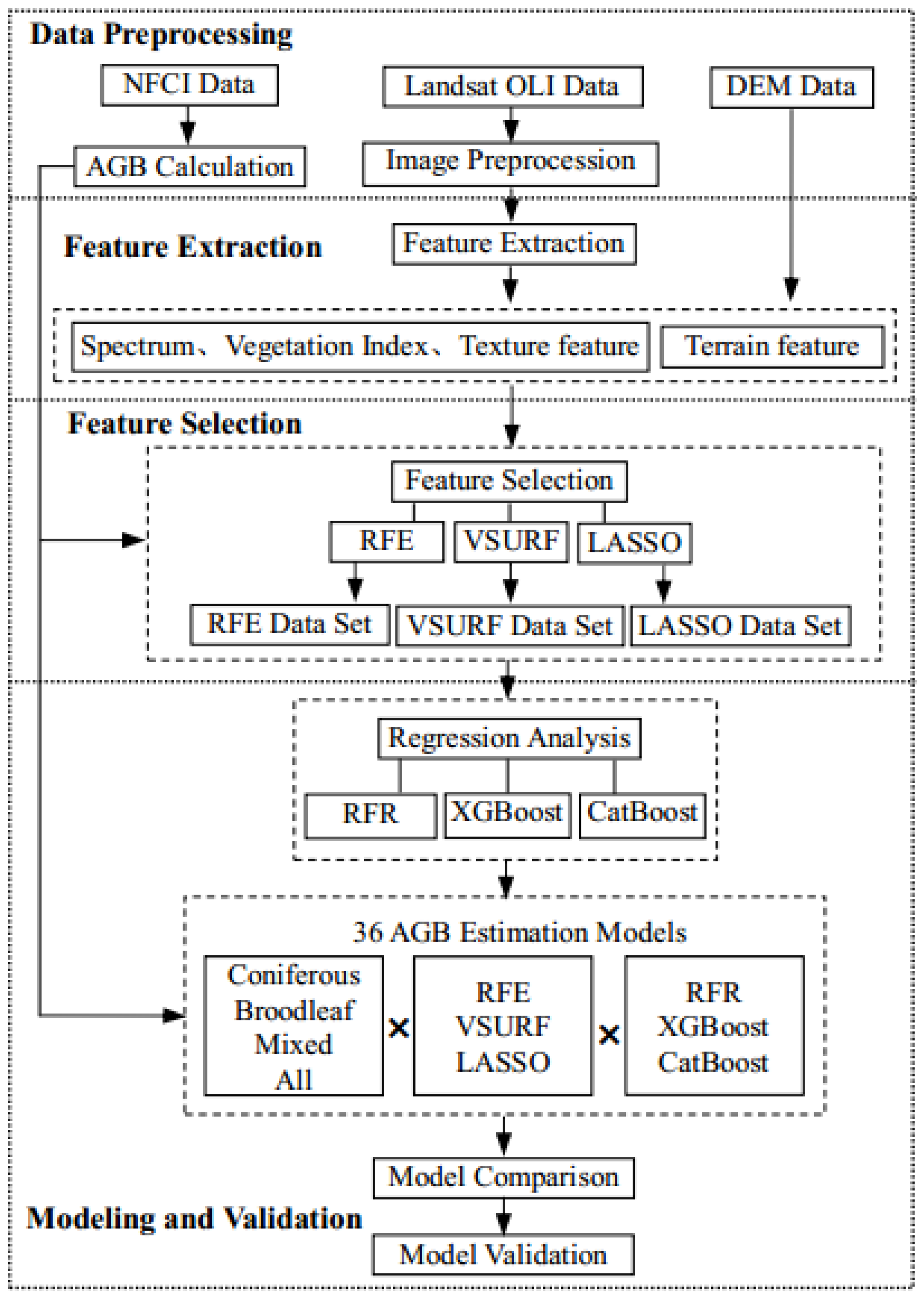
Compare and analyze AGB prediction models of different forest types by combining three feature selection methods (recursive feature elimination (RFE), variable selection using random forests (VSURF) and least absolute shrinkage and selection operator (LASSO)) and three regression algorithms (random forest regression (RFR), XGBoost, and CatBoost);

(2)

Evaluate the accuracy of the CatBoost algorithm for AGB estimation and compare it with the RFR and XGBoost algorithms;

(3)

Identify the best input variables for AGB estimation by feature selection.

2. Materials and Methods

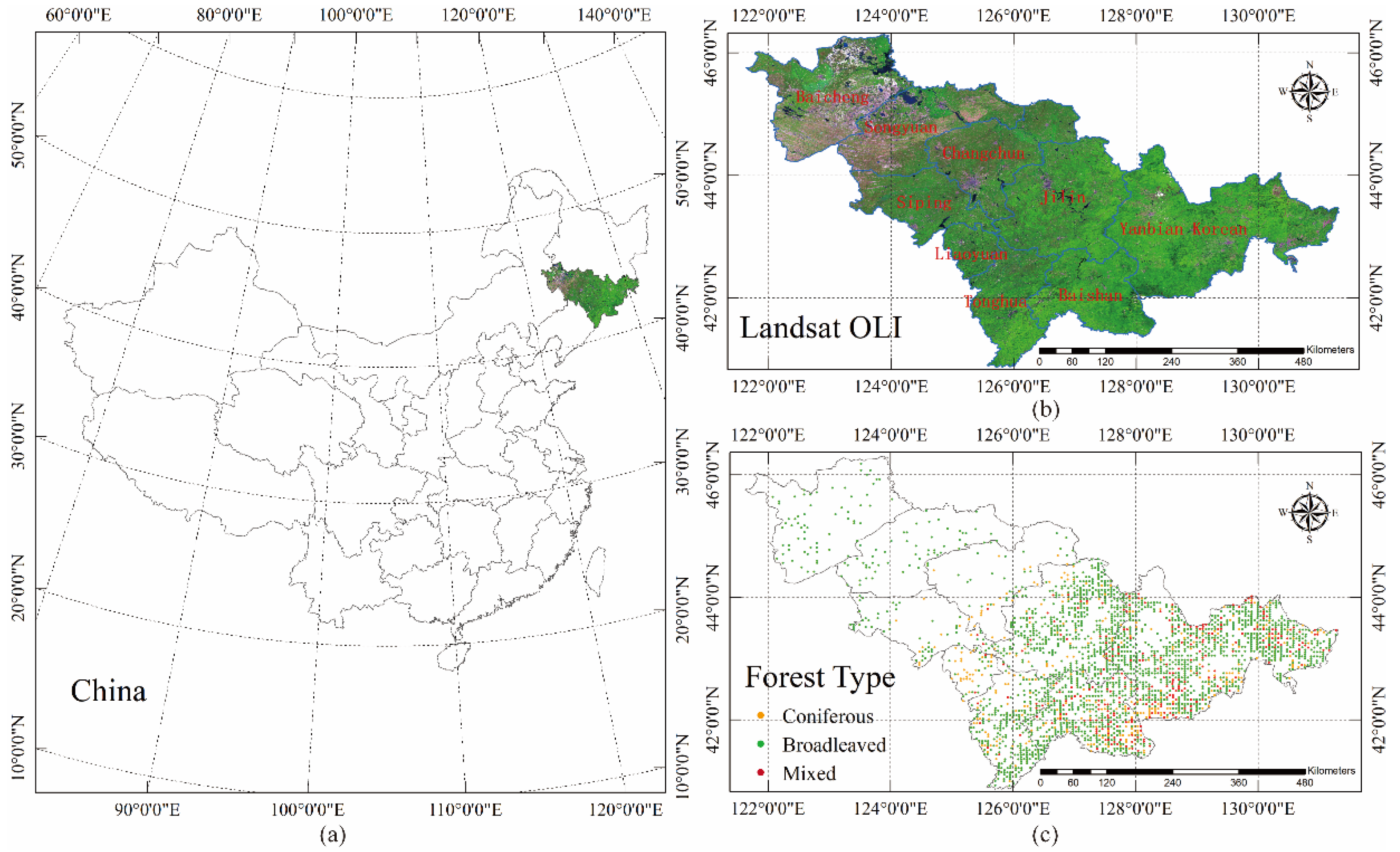
The methodological framework of this study consists of four steps: (1) data preprocessing, (2) feature extraction, (3) feature selection, and (4) modeling and validation (Figure 1).

2.1. Study Area

The study was conducted across all of Jilin province (19.1 × 104 km², 40°52′ N–46°18′ N, 121°38′ E–131°19′ E) in the central part of northeast China (Figure 2). It is characterized by hilly topography in the east and plains in the central region, and its elevation ranges from 279 to 2691 m [39]. Jilin has a temperate continental monsoon climate, with a more humid climate to the southeast and a semiarid climate in the northwest. The annual mean temperature is about 5.0 °C, with a maximum temperature of 23 °C in July and a minimum temperature of −20 °C in December. The seasonal distribution of precipitation is uneven: annual precipitation ranges from 400 to 600 mm, and 80% falls in the rainy season from June to September [40]. Natural forests form the bulk of the AGB studied in Jilin, and plantations are less common. The coniferous species are dominated by Pinus koraiensis Sieb. et. Zuccarini., followed by Picea asperata Mast. and Pinus sylvestris var. mongolica Litv. [41]. The major broadleaved species include Quercus mongolica Fischer ex Ledebour, Betula platyphylla Suk., Juglans mandshurica Maxim., Populus ussuriensis Kom., and Tilia amurensis Rupr [42].

2.2. Data Collection and Preprocessing

2.2.1. Field Data Collection and Preprocessing

This study made use of the ninth NFCI data of Jinlin Province collected in 2014. Square sampling plots with an area of 0.06 hectares were arranged at 4 km × 8 km grid intersection points along a system of vertical and horizontal coordinates. Tree heights, diameter at breast height (DBH) of all trees greater than 5 cm, canopy density, slope, aspect, and slope position were measured. Plot types, land types, age group, and dominant tree species were also recorded. Plots that were not on forested land (cropland, water, urban land, and bare land) and those covered by clouds in the remote sensing images were excluded. The final dataset included 2716 plots (Figure 2).

A continuous function was used to calculate the plot AGB, which was converted to per hectare biomass (Mg/ha) [43,44]. The regression equation is as follows:

$$B=\mathrm{a}V+\mathrm{b}$$

(1)

where B is biomass per unit area (Mg/ha); V that is the stock volume per unit area (m³/ha), was calculated according to the standing volume table method [45], and a and b are parameters whose specific values are given in

Table 1. The parameters of conversion model between AGB and forest stock volume [44].

Species/Species Group	a	b
Betula platyphylla Suk.	1.0687	10.2370
Pinus sylvestris var. mongolica Litv., Pinus densiflora Sieb. et Zucc.	1.0945	2.0040
Pinus thunbergii Parlatore	0.5168	33.2378
Pinus koraiensis Siebold et Zuccarini	0.5185	18.2200
Larix gmelinii (Ruprecht) Kuzeneva	0.6069	33.8060
Picea asperata Mast.	0.4642	47.4990
Populus simonii var. przewalskii (Maxim.) H. L. Yang	0.4754	30.6034
Pinus tabuliformis Carriere	0.7554	5.0928
Quercus	1.1453	8.5473
Mixed coniferous broad-leaved forest	0.8136	18.4660
Mixed broad-leaved forest	0.6255	91.0013

.

According to the technical regulations for the continuous forest inventory of China, the plots were classified into three types (coniferous forest, broad-leaved forest, and mixed forest) based on the standing volume of tree species (

Table 2. Classification standard of forest types [23].

Forest Type	Abbreviation	Standard of Division
Coniferous forest	Coniferous	Pure coniferous forest (single coniferous species stand volume ≥ 65%); coniferous mixed forest (coniferous species total stand volume ≥ 65%)
Broad-leaved forest	Broadleaf	Pure broadleaf forest (single broad-leaved species stand volume ≥ 65%); broadleaf mixed forest (broad-leaved species total stand volume ≥ 65%)
Mixed forest	Mixed	Broadleaf–coniferous mixed forest (total stand volume of coniferous or broad-leaved species accounting for 35%–65%)

) [23]. The AGB values of all plots (abbreviated as “All” in tables and figures) ranged from 19.20 Mg/ha to 309.58 Mg/ha with an average of 153.8Mg/ha and a standard deviation of 49.58 Mg/ha. The average AGB values of coniferous, broadleaf, and mixed plots were 103.32, 155.60, and 186.86 Mg/ha, respectively (

Table 3. Distribution of the plot AGB values (Mg/ha) of the different forest types.

Figure	Count	Minimum (Mg/ha)	Maximum (Mg/ha)	Mean (Mg/ha)	Standard Deviation	Sample Size (Training)	Sample Size (Validation)
Coniferous	358	20.41	286.34	103.32	52.90	269	89
Broadleaf	2111	19.20	269.80	155.60	47.14	1583	528
Mixed	247	91.67	309.58	186.86	38.15	185	62
All	2716	19.20	309.58	153.80	49.58	2037	679

).

2.2.2. Remote Sensing Data Collection and Preprocessing

The remote sensing data used in this study were acquired from the Landsat OLI satellite and included one band in the panchromatic mode and eight bands in the multispectral mode. Landsat OLI images with cloud cover less than 5% were acquired on the GEE platform (https://earthengine.google.com/, accessed on 15 May 2020) from June to September of 2014. Data preprocessing steps were performed on the GEE platform, including radiation correction, terrain correction, cloud removal, image splicing, and atmospheric apparent reflectance conversion [46]. A total of 18 Landsat OLI images were obtained, covering the entire study area. Band 1-coastal and band 9-Cirrus were excluded, as Band 1 and Band 9 are used as indicators of coastal zone observation and cloud detection, respectively. Although the images were resampled to a pixel size of 25.82 m, the same size as the inventory plot, there are certain positional offsets between the boundary of the sample site and the remote sensing image. To reduce the impact of these positional offsets, a buffer zone with a radius of 25.82 m was established around each plot. Then, the mean pixels of each plot center buffer are extracted as the sample plot value.

2.3. Predictive Variables

A total of 53 predictive variables were extracted for this study (

Table 4. Summary of predictor variables including Landsat OLI spectral variables, vegetation indexes, texture measures, terrain factors, and forest factor for AGB estimation.

Variable Type	Variable Number	Variable Name	Description
Spectral variables	6	Band2, Band3, Band4, Band5, Band6, Band7	Landsat OLI Bands 2–7: Blue, Green, Red, NIR, SWIR1, SWIR2
Vegetation indexes	11	NDVI	Normalized Difference Vegetation Index
		RVI	Ratio Vegetation Index; RVI = NIR/RED
		DVI	Difference Vegetation Index
		RVI54	Ratio Vegetation Index 1; VI54 = SWIR1/NIR
		RVI64	Ratio Vegetation Index 2; VI64 = SWIR2/NIR
		SAVI	Soil Adjusted Vegetation Index
		NLI	Optimize soil adjustment index; NLI = (NIR^2-RED)/(NIR^2 + RED)
		ARVI	Atmospherically Resistant Vegetation Index
		EVI	Enhanced Vegetation Index
		TSAVI	Transformed Soil Adjusted Vegetation Index
		PVI	Perpendicular vegetation Index
Texture measures	32	TjMea, TjVar, TjHom, TjCon, TjDis, TjEnt, TjASM, TjCor	Panchromatic band of Landsat OLI texture measurement using gray-level co-occurrence matrix based on four window sizes
Terrain factors	3	Elevation, slope, aspect
Forest factors	1	Canopy density

Note: TjXXX represents a texture image developed in the Landsat panchromatic band using the texture measure XXX with a j × j (j = 3, 5, 7, 9) pixel window, where XXX is Mea (Mean), Var (Variance), Hom (Homogeneity), Con (Contrast), Dis (Dissimilarity), Ent (Entropy), ASM (Angular Second Moment), or Cor (Correlation).

). Six spectral variables were derived from the average surface reflectance of the six multispectral bands. Eleven vegetation indices that have been widely used in previous forest studies were calculated [47]. Texture measures were extracted using the gray level co-occurrence matrix method (GLCM) [48], and eight GLCM measures with four different window sizes (3 × 3, 5 × 5, 7 × 7, and 9 × 9) were calculated from the panchromatic band. Elevation, slope, and aspect were selected as terrain factors and were derived from a digital elevation model (DEM) with a spatial resolution of 30 m, which were downloaded from the United States Geological Survey (USGS) Earth Explorer (http://earthexplorer.usgs.gov/, accessed on 30 June 2019). Canopy density from field surveys was also used as a predictor variable, that is, the ratio of canopy projection area to woodland area.

2.4. Feature Selection Methods

Feature selection is one of the critical steps in machine learning and has two main functions: (1) reducing the number of features and dimensions, thereby enhancing model generalizability and reducing overfitting, and (2) enhancing the understanding between features and eigenvalues. RFE, VSURF, and LASSO were applied to the original dataset to determine the appropriate variable number.

2.4.1. Recursive Feature Elimination

RFE is a well-established wrapper method to find the optimal feature subset [49]; it repeatedly constructs models and finally selects the best predicted feature set. The best or worst features are removed on the basis of coefficients, and the remaining features are used to build the next model until all features have been used. Finally, the features are sorted according to their order of elimination. To determine the best number of features, a 10-fold cross-validation resampling method was added to RFE. The ‘rfe ()’ function in the ‘caret’ package (version: 6.0-84) was used to implement RFE on R 3.5.3, with ‘Repeatedcv’ for method, ‘5’ for repeats, and ‘random forests (rfFuncs)’ for functions.

2.4.2. Variable Selection Using Random Forests

VSURF is a wrapper-based algorithm that uses random forests as the base classifier [50]. Feature variables are first ranked based on a variable importance measure, and low-scoring features are eliminated to reduce the number of features and improve model accuracy [51]. In the final step, a ranked list of only the most important features is produced.

2.4.3. Least Absolute Shrinkage and Selection Operator

LASSO was introduced by Robert Tibshirani [52]. On the basis of linear regression, the algorithm constrains the absolute value of the model regression coefficient to a specific threshold and minimizes the sum of squares of model residuals by increasing the normal form function. By optimizing the objective function, variables whose correlation is less than the threshold value are compressed to 0 and eliminated, leaving only the remaining preferred variables. The ‘cv.glmnet’ function of the ‘glmnet’ package (version: 2.0-18) of R is used for LASSO feature selection. ‘cv.glmnet’ uses a 10-fold cross-validation method for verification, which is more suitable for feature selection with high-dimensional data.

2.5. Machine Learning Algorithms

2.5.1. Random Forest Regression

RFR is an ensemble learning technique proposed by Breiman in 2001 [53]. This multiple decision tree algorithm is based on classification and regression trees and is controlled by the number of decision trees (Ntree) and the number of nodes (Mtry) [54]. The complexity of the model is directly proportional to Ntree. Therefore, if prediction accuracy is similar, a smaller Ntree is better than a larger Ntree. Mtry controls the degree of randomness introduction, and its value is generally one-third of the number of input variables in the regression model [55,56]. The optimal variables are selected through successive modeling calculations. RFR has the advantages of processing high-dimensional data, avoiding overfitting, and ranking the importance of features.

2.5.2. Extreme Gradient Boosting

XGBoost is a boosting algorithm proposed by Chen et al. in 2016 based on the GBDT and RF approaches [57]. Compared with GBDT, XGBoost has improvements in multithreaded processing, the classifier, and the optimization function [58]. It also has the following advantages [59,60]:

(1)

The algorithm controls the complexity of the tree and then reduces overfitting by adding a regularization term to the objective function.

(2)

A column sampling technique is employed to prevent overfitting, similar to the random forest algorithm.

(3)

The second-order Taylor expression of the objective function is used to make the definition of the objective function simpler and more precise when finding the optimal solution.

2.5.3. Categorical Boosting

CatBoost was developed by Dorogush et al. in 2018 [61] and is an improved GBDT toolkit similar to XGBoost. CatBoost solves the problems of gradient bias and prediction shift [33]. It has several advantages [34,62]:

(1)

An innovative algorithm is embedded to automatically treat categorical features as numerical characteristics.

(2)

It uses a combination of category features that take advantage of the connections between features, greatly enriching feature dimensions.

(3)

A perfectly symmetrical tree model is adopted to reduce overfitting and improve the accuracy and generalizability of the algorithm.

RFR, XGBoost, and CatBoost modeling were performed with the R packages ‘randomForest’, ‘XGBoost’, and ‘CatBoost’, respectively. The ‘Caret’ package (version: 6.0-84) was used to optimize model parameters.

2.6. Evaluation of AGB Estimation Accuracy

First, data were preprocessed before modeling. Any data point that is more than 3 standard deviations is an outlier. At the same time, we also carefully removed outliers based on experience. To improve the convergence speed and model accuracy, the data was min-max normalized so that the resulting values were mapped to between 0 and 1 and formula is as Equation (2). Next, 10-fold cross-validation was used to optimize the parameters for all algorithms (RFR, XGBoost, and CatBoost) based on the training dataset (75% of the data). Finally, the calibrated model from 10-fold cross-validation was tested once again with the independent validation dataset (25% of the data) to estimate the root mean square error (RMSE), coefficient of determination (R²), relative RMSE (RMSE%), and bias of the models. The formulas for these statistical parameters are as follows:

$$x_j=\frac{x_i-x_{\min }}{x_{\max }-x_{\min }}$$

(2)

$$R^2=1\sum \frac{{\displaystyle \sum _{i=1}^n{\left(y_i-{\widehat{y}}_i\right)}^2}}{{\displaystyle \sum _{i=1}^n{\left(y_i-\overline{y}\right)}^2}}$$

(3)

$$\mathrm{RMSE}=\sqrt{\frac{{\displaystyle \sum _{i=1}^n{\left(y_i-{\widehat{y}}_i\right)}^2}}{N}}$$

(4)

$$\mathrm{RMSE}\%=\frac{\mathrm{RMSE}}{\overline{y}}\ast 100$$

(5)

$$\mathrm{Bias}=\frac{{\displaystyle \sum _{i=1}^n{\left(y_i-{\widehat{y}}_i\right)}^{}}}{N}$$

(6)

where $x_i$ is the data before normalization, $x_j$ is the normalized data, $x_{\min }$ is the minimum value of sample data, and $x_{\max }$ is the maximum value of sample data. ${\widehat{y}}_i$ is the predicted value, $y_i$ is the observed value, $\overline{y}$ is the mean of the observed values, and N is the number of observations.

3. Results

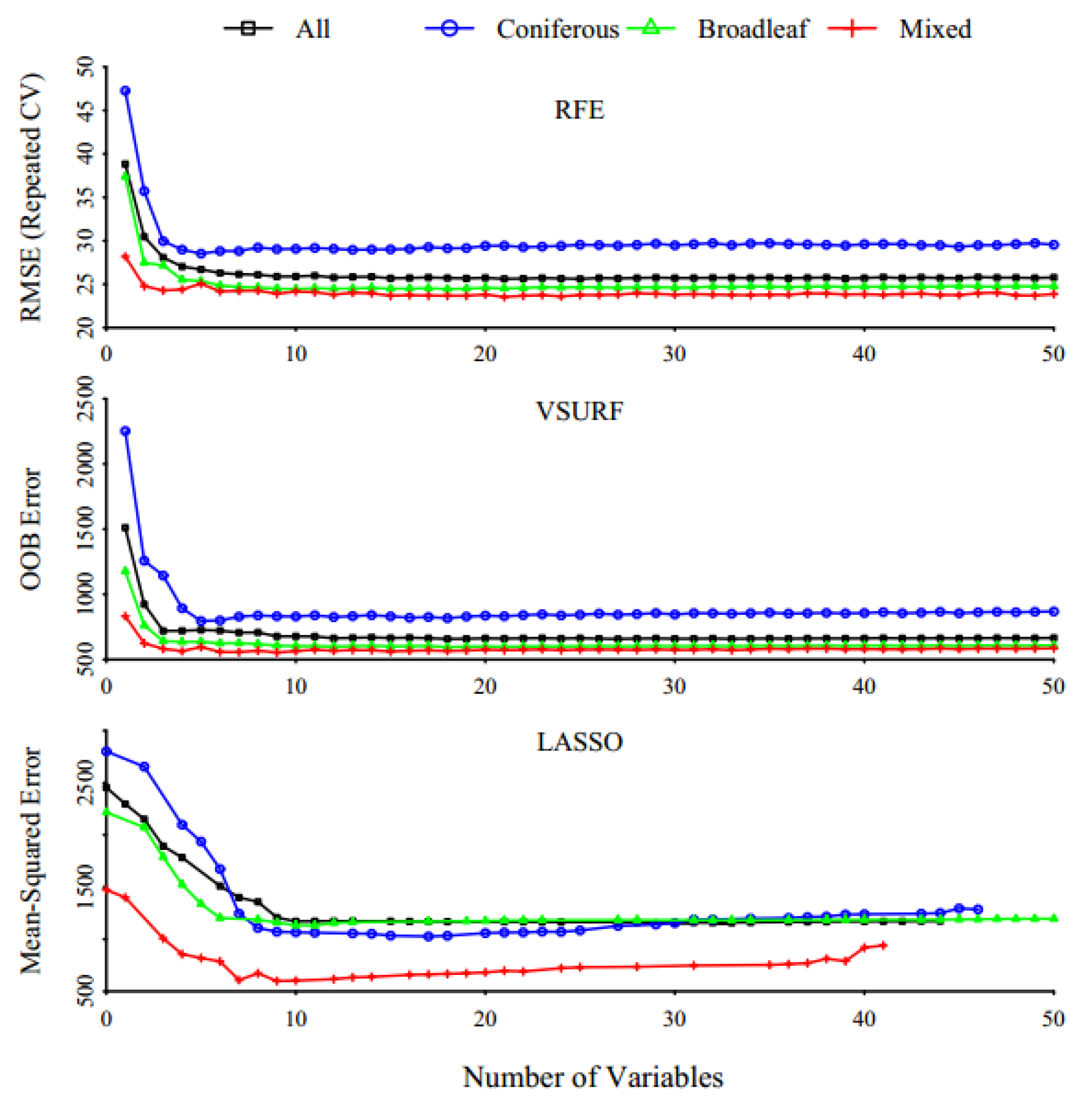
3.1. Determining the Optimal Number of Variables

Different forest types showed different RMSE trends as the input variable number changed in the RFE feature selection method (Figure 3). The number of selected features differed among the different forest types. For coniferous forest, the optimal number of features was five, whereas 10, 21, and 25 features were selected for the broadleaf forest, the mixed forest, and all forests.

For VSURF, the OOB error values decreased continuously as the variable number increased from 0 to 20 but changed only slightly as the variable number increased from 20 to 52. The variation trend for LASSO was similar to that of VSURF. After comprehensive consideration, 20 was a suitable variable number that maintained most of the information from the original dataset, and VSURF and LASSO selected the top 20 features with the highest scores.

3.2. Predictive Performance Using Feature Selection

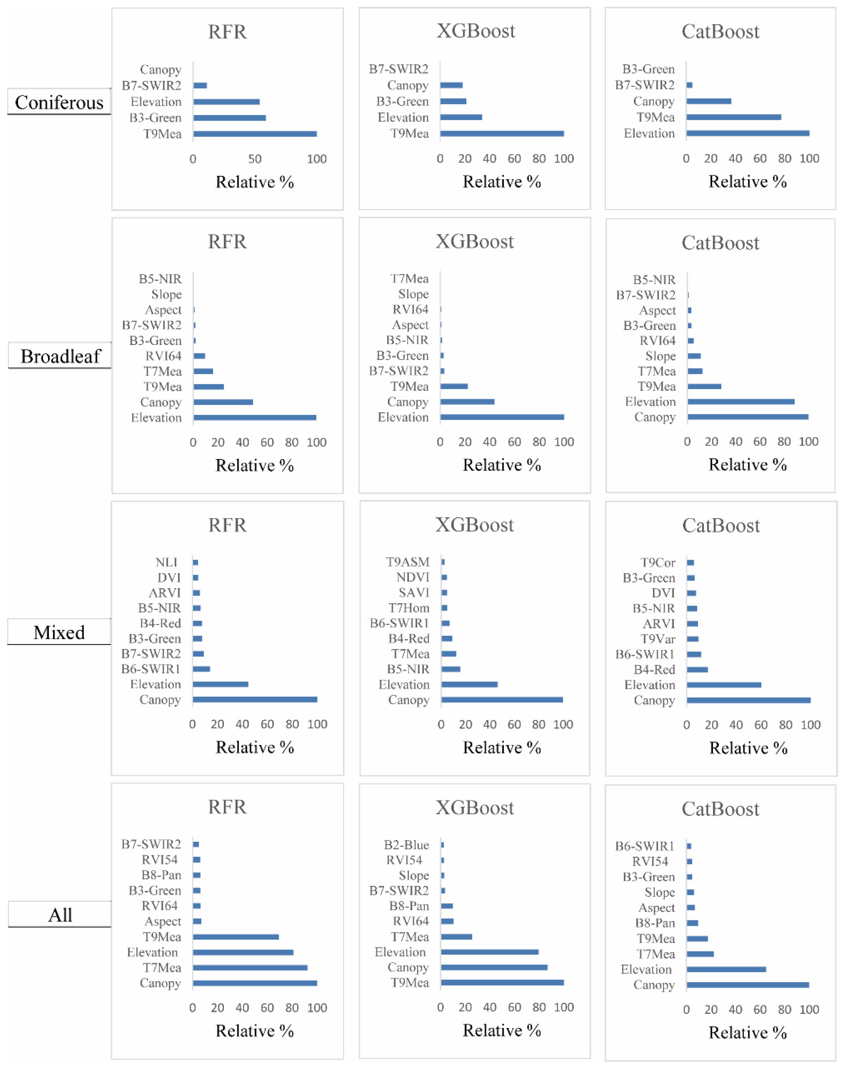
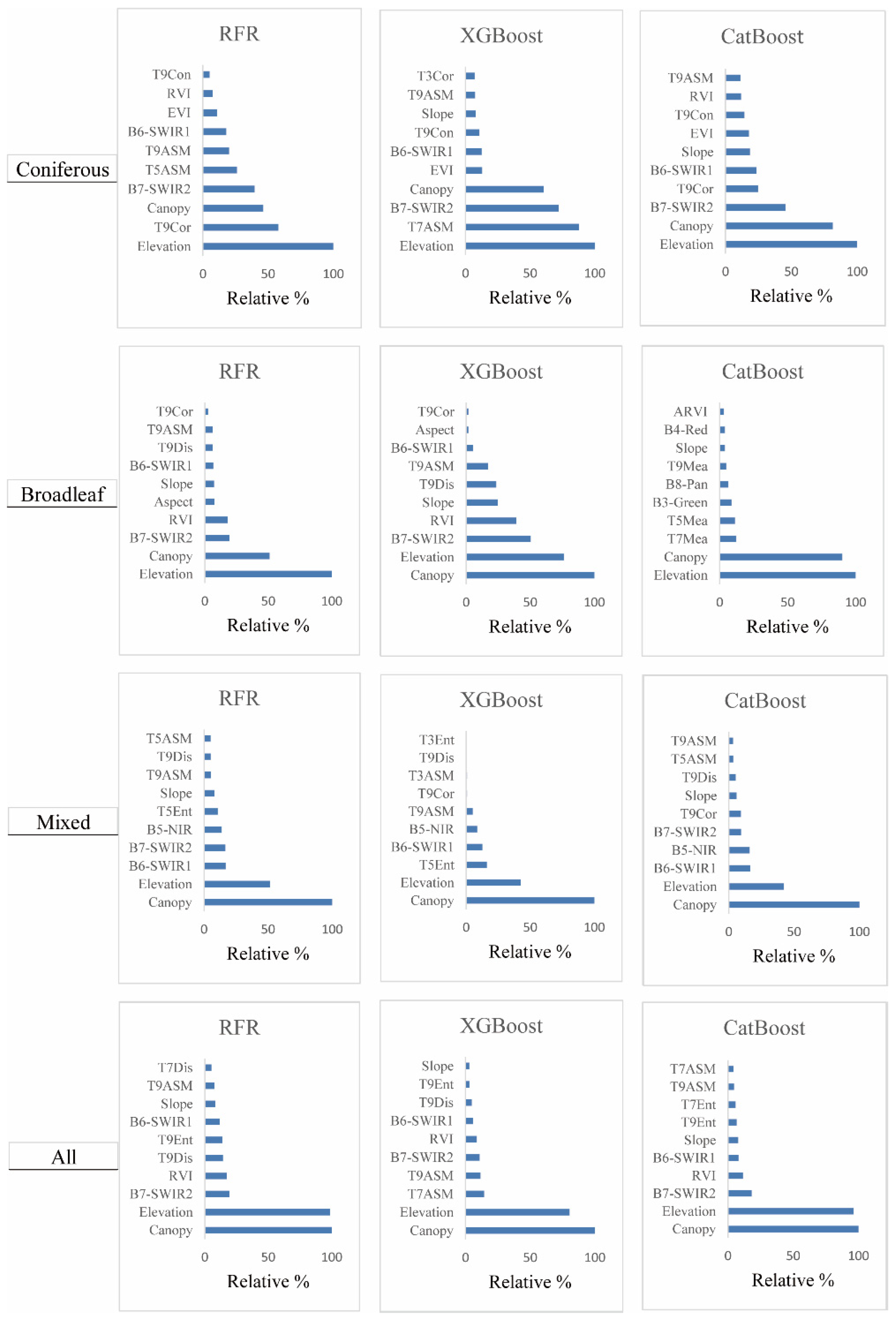
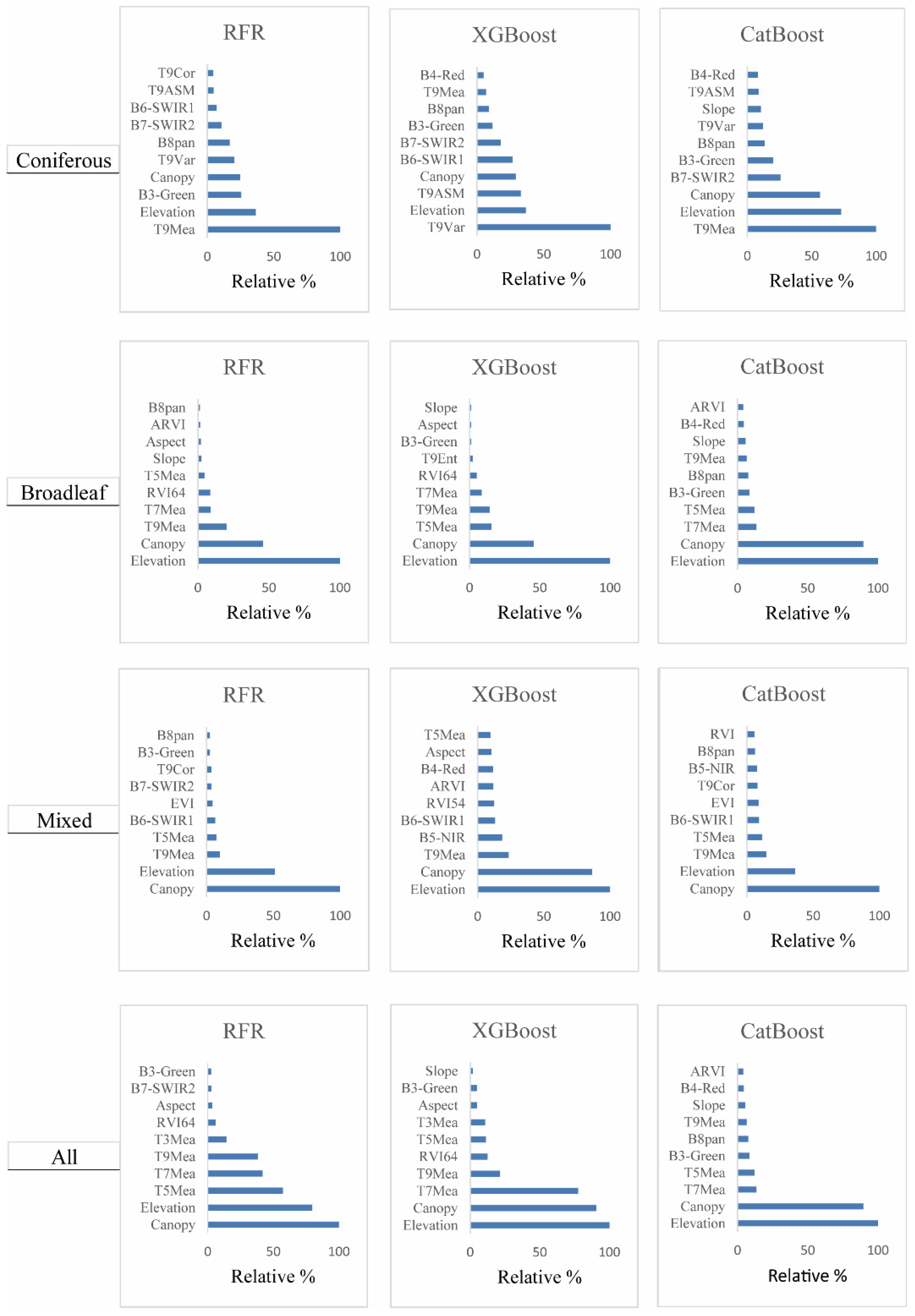
3.2.1. Variable Importance Measures

We calculated Pearson correlation coefficients between the predictor variables and AGB and found that the T9Mea texture measure had the highest correlation coefficient (−0.61). The correlation coefficients between most texture measures and AGB were 0.2–0.5. Band4 (red) had the highest correlation with AGB among the spectral variables, with a value of −0.57. RVI64 had the highest correlation with AGB among the vegetation indexes, with a value of −0.54. The correlation coefficients of elevation, slope, and canopy density with AGB were 0.56, 0.46, and 0.24, respectively.

The AGB models constructed by combining different feature selection methods (RFE, VSURF, LASSO) and machine learning algorithms (RFR, XGBoost, CatBoost) had different orders of feature importance. Figure 4 shows the top 10 selected prediction features based on feature importance for the different forest types obtained with the RFE feature selection method and the three machine learning algorithms. Spectral variables, vegetation indexes, texture measures, terrain factors, and the forest factor were included in most of the AGB models for all forests (All), although the specific selected variables differed. This result indicated that multiple features, rather than a single feature, influenced AGB estimation.

Five features were selected in the coniferous forest model: T9Mea, B3-Green, Elevation, B7-SWIR2, and Canopy. T9Mea, Elevation, and Canopy were also frequently selected for the AGB models of broadleaf forest, indicating that these features have significant roles in AGB estimation. Canopy and elevation were the two most important features in all mixed forest models. In AGB models of all forests, the three most important variables were Canopy, T7Mea, and Elevation for the RFE-RFR model; T9Mea, Canopy, and Elevation for the RFE-XGBoost model; and Canopy, Elevation, and T7Mea for the RFE-CatBoost model. Canopy and Elevation were included in all AGB models, indicating that both features contained sufficient information to enhance the performance of AGB estimation models.

Textures based on 7 × 7 and 9 × 9 window sizes were frequently involved in the models, indicating that these two window sizes were more appropriate for AGB estimation. Window size is an important factor that affects the accuracy of the AGB estimation model. Small windows are more sensitive to the pixel difference between canopy and shadow ratio, whereas large windows cannot extract sufficient texture information due to the excessive smoothness phenomenon of texture parameters. Mean texture was frequently involved in the model, indicating that Mean contributed more than other texture measures.

Figure A1 presents the rankings of the top 10 AGB model variables obtained when LASSO was combined with the machine learning algorithms, and Figure A2 presents the results obtained when VSURF was used. Similar to RFE, all types of features (spectral variables, vegetation indexes, texture measures, terrain factors, and the forest factor) were involved in the AGB models when LASSO and VSURF were used for feature selection. However, the specific variables selected were different. Spectral variables, vegetation indexes, and texture measures played different roles in the AGB models of broadleaf, mixed, and coniferous forests. The spectral and vegetation index variables could be used to distinguish broadleaf and mixed forests, owing to their diversity of tree species and multiple canopy layers. By contrast, because the coniferous forest was dominated by a small number of species, its AGB could be explained well by texture rather than spectral information. It was interesting to note that canopy density contributed significantly to the models for most forest types, especially in broadleaf and mixed. This likely reflects the fact that forest canopy structure was complex and diverse.

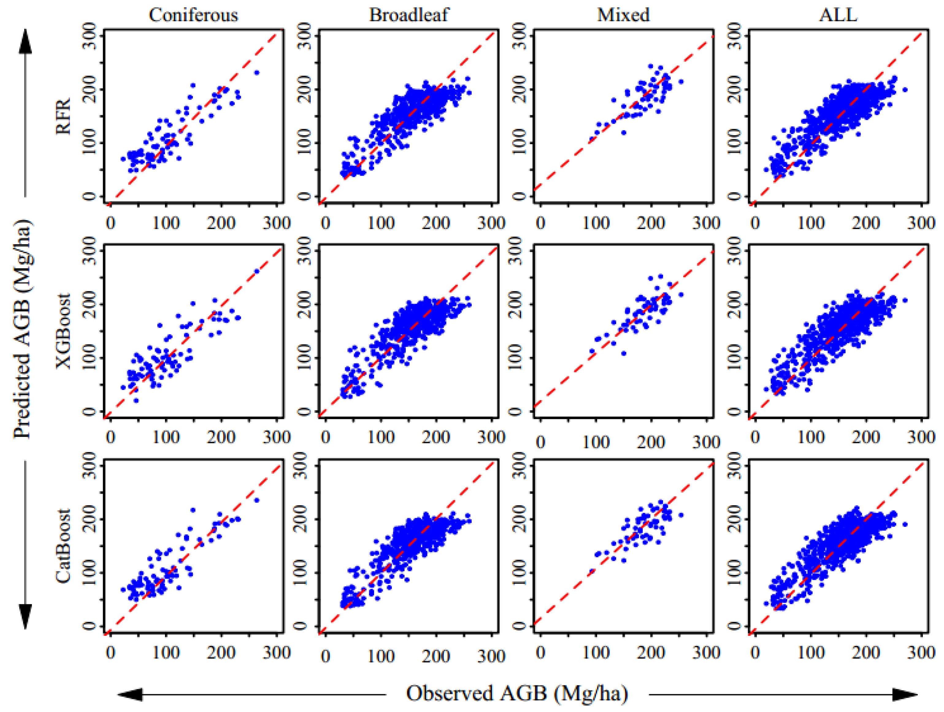
3.2.2. Comparison of Model Performance

The key tuning hyperparameters and the configurations of the tuning parameters for 36 AGB models are shown in

Table A1. Optimal hyperparameter using a grid search with 10-fold CV for the different AGB models.

Method	Forest Type	CatBoost		XGBoost		RFR
		Depth	Learning Rate	Max Depth	Eta	Mtry
LASSO	Coniferous	6	0.049787	2	0.3	17
	Broadleaf	6	0.049787	2	0.3	9
	Mixed	6	0.049787	1	0.3	12
	All	4	0.135335	2	0.3	9
RFE	Coniferous	4	0.049787	1	0.4	2
	Broadleaf	6	0.049787	2	0.3	4
	Mixed	4	0.135335	1	0.3	10
	All	4	0.135335	3	0.3	9
VSURF	Coniferous	2	0.135335	2	0.3	14
	Broadleaf	6	0.135335	2	0.3	12
	Mixed	4	0.135335	2	0.3	20
	All	4	0.135335	3	0.3	12

Note: In CatBoost models, iterations = 100 for all feature selection methods. In the XGBoost model, nrounds = 50, gamma = 0 for all feature selection methods.

. Three machine learning algorithms, RFR, XGBoost, and CatBoost, were used to fit the modeling dataset based on the RFE feature selection method, and the results are presented in

Table 5. AGB estimation accuracy assessments on validation dataset by combining RFE with machine learning algorithms (CatBoost, XGBoost, RFR) for different forest types.

Forest Type	Model	R2	RMSE (Mg/ha)	Bias (Mg/ha)	Relative RMSE (%)	Run Times (min)
Coniferous	CatBoost	0.77	26.54	−5.56	25.62	0.78
	XGBoost	0.72	28.81	−2.15	27.81	20.17
	RFR	0.77	26.63	−5.88	25.70	0.17
Broadleaf	CatBoost	0.73	24.67	0.63	15.84	1.36
	XGBoost	0.71	25.55	0.10	16.40	25.13
	RFR	0.73	24.74	0.13	15.87	5.37
Mixed	CatBoost	0.59	22.62	2.14	12.10	1.51
	XGBoost	0.60	22.44	0.20	12.01	20.14
	RFR	0.59	22.72	1.81	12.16	0.63
All	CatBoost	0.73	25.77	−0.86	16.80	1.81
	XGBoost	0.72	26.21	−0.91	17.08	29.81
	RFR	0.72	26.13	−0.93	17.04	12.55

. Comprehensive consideration based on the accuracy indicators (R², RMSE, RMSE%, and Bias), CatBoost was the best machine learning algorithm. For the coniferous forest, the CatBoost algorithm produced more accurate estimates (with RMSE of 26.54 Mg/ha) than the RFR (with RMSE of 26.63 Mg/ha) and XGBoost (with RMSE of 28.81 Mg/ha) algorithms. CatBoost also achieved the lowest RMSE values for different forest types except for mixed forest compared with the other algorithms. Interestingly, sometimes the Bias of the RFR is lower than CatBoost. One possible explanation is that the positive and negative predicted values cancel each other out in the RFR algorithm. The ensemble learning algorithms (XGBoost and CatBoost) have shown potential in fields such as biology and medicine [13,33,34,35,36]. Here, we found that CatBoost turns out to be a promising method for modeling forest AGB using remote sensing data.

Table 6. AGB estimation accuracy assessment on validation dataset by combining LASSO with machine learning algorithms for different forest types.

Forest Type	Model	R2	RMSE (Mg/ha)	Bias (Mg/ha)	Relative RMSE (%)	Run Times (min)
Coniferous	CatBoost	0.73	28.12	−3.35	27.14	1.59
	XGBoost	0.74	28.30	−5.50	27.31	20.91
	RFR	0.73	28.24	−4.09	27.25	0.77
Broadleaf	CatBoost	0.72	25.11	0.83	16.11	2.05
	XGBoost	0.70	26.16	0.79	16.79	28.79
	RFR	0.71	25.54	0.36	16.39	8.26
Mixed	CatBoost	0.60	22.73	1.05	11.10	1.51
	XGBoost	0.57	23.73	2.64	12.70	19.78
	RFR	0.58	23.18	1.12	11.66	0.35
All	CatBoost	0.71	26.65	−0.97	17.37	1.85
	XGBoost	0.69	27.73	−0.74	18.08	28.11
	RFR	0.71	26.81	−1.24	17.48	10.74

presents the estimate accuracy of AGB models in which LASSO was combined with the machine learning algorithms, and

Table 7. AGB estimation accuracy assessment on validation dataset by combining VSURF with machine learning algorithms for different forest types.

Forest Type	Model	R2	RMSE (Mg/ha)	Bias (Mg/ha)	Relative RMSE (%)	Run Times (min)
Coniferous	CatBoost	0.74	27.72	−4.91	26.76	1.72
	XGBoost	0.73	28.51	−5.17	27.52	19.62
	RFR	0.75	27.44	−4.04	26.49	0.78
Broadleaf	CatBoost	0.73	24.77	0.49	15.89	1.85
	XGBoost	0.71	25.62	0.67	16.44	28.90
	RFR	0.72	25.08	0.88	16.09	9.01
Mixed	CatBoost	0.59	22.89	0.76	12.25	1.20
	XGBoost	0.56	23.69	1.03	12.68	17.45
	RFR	0.57	23.20	2.30	12.42	0.48
All	CatBoost	0.74	25.79	−1.15	16.67	3.18
	XGBoost	0.72	26.25	−0.68	17.11	36.82
	RFR	0.72	26.12	−0.94	17.03	12.18

presents the results obtained using VSURF. For all forest types, models that used RFE-based selection clearly performed better than models that used VSURF or LASSO. For example, for broadleaf, the RMSE of VSURF-selected models (24.77, 25.62, and 25.08 Mg/ha) and LASSO-selected models (25.11, 26.16, and 25.54 Mg/ha) were much larger than those of RFE-selected models (24.67, 25.55, and 24.74 Mg/ha). These results indicate that the RFE-selected dataset retained more useful information from the original dataset, thereby explaining the differences in AGB estimation. The best AGB model predictions were obtained when RFE was combined with the CatBoost algorithm. Moreover, the RFE–CatBoost model (RFE used for feature selection and CatBoost used for regression) performed well in prediction accuracy compared to the VSURF-RFR model (in which random forests were used for both feature selection and regression) for all forest types. This result indicates that the typical method of simultaneous feature selection and regression with the same machine learning algorithm may not always ensure an optimal estimate. The combination of different feature selection and regression algorithms was helpful in improving the accuracy of the AGB model.

3.3. Evaluation of AGB Estimation

The scatter plots shown in Figure 5 illustrate the relationships between predicted and observed AGB for different forest types using the RFR, XGBoost, and CatBoost algorithms with the RFE variable selection method. The CatBoost algorithm was superior to the RFR and XGBoost algorithms. Within a given algorithm, the accuracy of the broadleaf model is the highest, followed by the all and mixed models, the coniferous model being the least accurate.

4. Discussion

Feature selection methods and machine learning algorithms were effective tools for improving the accuracy of AGB estimates. To predict the AGB of four forest types, 36 models were derived using three feature selection methods (RFE, VSURF, and LASSO) and three machine learning algorithms (RFR, XGBoost, and CatBoost) based on NFCI data. CatBoost performed well in the prediction of all forest types compared to XGBoost and RFR. AGB models were most accurate when RFE was used for feature selection, and this method worked better than VSURF or LASSO. The combination of RFE feature selection with the CatBoost algorithm effectively improved the accuracy of AGB estimates. Since feature selection can reduce data dimensionality, minimize data storage space, and improve model interpretability, it has been employed to improve the performance of predictive models. RFE showed the smallest RMSE, followed by VSURF and LASSO. The first five features selected for the RFE-RFR-Broadleaf model were Elevation, Canopy, T9Mea, RVI64, and B3-green. This result demonstrated that the feature selection method effectively selected different types of features, including spectral variables, vegetation indexes, texture measures, terrain factors, and the forest factor, confirming its applicability and effectiveness for AGB estimation from multispectral data. In this study, there is a high correlation between the Mean texture and AGB. It seems likely that these results are in fact due to the reflection of the regularity of the image texture in the Mean texture. The image texture rules of different tree species are quite different; thus, the average image texture can better reflect the tree species diversity in the study area. The Mean texture contains the information on the species of the tree and is beneficial to the diversity prediction of the forest tree species, which is consistent with the finding of Li et al. [63]. Canopy density was proved to have an effect on the accuracy of the AGB estimation. There are many types of trees in the study area, and the variance in the growth status of those tree species leads to the change in the canopy density. A high canopy density can be attributed to the lush of the forest and a high AGB. In a study conducted by Li et al. [63], AGB and LAI were estimated based on digital aerial photograph data in northeast China. When the results were analyzed, it was found that the canopy density extracted from photogrammetric point cloud is the most strongly related to the estimated LAI. However, the underlying mechanisms and relationships should be studied in more detail in the future. The results of the present study agree to a large extent with those of previous studies [6,7,13]. The feature selection capability of RFE has been reported in recent studies of halophyte biomass estimation based on WorldView-2 multispectral data (Rasel et al. [7].) and forest parameter prediction using optical data (Dan Li et al. [63]). The VSURF feature selection method implements a feature selection function by measuring the importance of features [18]. Specifically, it produces a set of feature scores ranked from largest to smallest, rather than an optimal feature combination. A feature set is the final result of RFE, which more fully conveys the information from the original dataset. In addition, the stability of RFE was enhanced owing to the use of “random forests” as the underlying model for RFE during iteration.

The application of machine learning algorithms to optical data processing in quantitative remote sensing is developing rapidly. However, there have been few applications of new ensemble learning algorithms to AGB estimation. Here, the CatBoost algorithm was shown to be superior to XGBoost, but it was only slightly superior to RFR. The RFR algorithm, a parallel integrated algorithm, is not sensitive to predictive variables that contain noise, as the decision tree is independent [64,65]. The decision tree of XGBoost is generated based on the previous tree and improves the processing of regularized learning targets to avoid overfitting [60]. In contrast to XGBoost, CatBoost can avoid overfitting by adding an algorithm to compute leaf nodes when choosing a tree structure [62]. Consequently, CatBoost not only performed well on the validation set but also had the lowest degree of overfitting on the validation set. For example, the RFE-ALL-RFR (R² = 0.96, RMSE = 10.50 Mg/ha) model outperformed RFE-ALL-CatBoost (R² = 0.81, RMSE = 21.76 Mg/ha) in the training dataset, but RFE-ALL-CatBoost (R² = 0.73, RMSE=25.77 Mg/ha) turned out to be better than RFE-ALL-RFR (R² = 0.72, RMSE = 26.13 Mg/ha) in the validation dataset. CatBoost also had a faster run time than XGBoost, thus improving the efficiency of the operation. In addition, CatBoost works faster in large samples. In the coniferous (n = 358) and mixed (n = 247), RFR was slightly faster than CatBoost. However, in broadleaf (n = 2111) and ALL (n = 2716), CatBoost runs much faster than RFR (Table 5, Table 6 and Table 7). This finding is in line with the results reported by Zhang et al., which show that the CatBoost algorithm outperformed the RFR and GBRT algorithms for the AGB estimation [37]. Li et al. focused on the potential for machine learning algorithms to improve AGB estimation accuracy [23]. Interestingly, our results showed only a slight difference in prediction performance between XGBoost and RFR, whereas Li et al. reported better results for XGBoost. The different feature selection method used in our study may explain the differences in our results.

The AGB prediction models based on a combination of different feature selection methods and machine learning algorithms were superior to those in which one machine learning algorithm was used for both feature selection and regression. For example, the RFE-CatBoost-Coniferous model (RMSE = 26.54 Mg/ha) outperformed the VSURF-RFR-Coniferous model (RMSE = 27.44 Mg/ha). Previous studies on LAI estimation also reported that using the same machine learning algorithm for both feature selection and regression was not always the optimal solution. It is interesting to note that Chen et al. found the VSURF-RFR model to be the best, although in this case, the study object and the method of comparison were different [38]. Overall, our experiment indicates that using the same machine learning algorithm for feature selection and regression does not improve AGB estimation accuracy. There are two likely causes for such a result. One possible explanation for this might be that the scores are adopted by the RF algorithm as the criterion for feature selection. However, most of the scores only represent the correlation between one particular input variable and the AGB. Therefore, it does not guarantee that the combination of variables with high scores would be the optimal choice for AGB estimation. Additionally, the feature selection process was conducted twice duo to the employment of the combination of the feature selection method and the regression algorithm.

Here, the combination of CatBoost algorithm and feature selection methods was applied to AGB prediction for the first time and achieved the best performance. In this regard, the combination of different feature selection methods and regression algorithms can be considered as a powerful tool in AGB prediction. This tool could be extended to other fields of forest ecology, for example, predicting other biophysical parameters (leaf area index, forest canopy coverage rate, and effective canopy coverage rate), soil nutrient or soil heavy metal content using optical and hyperspectral remote sensing data. To some readers, machine learning methods (especially neural networks) seem like a black box. The three machine learning algorithms (RFR, XGBoost, and CatBoost) selected in our study are easier to understand in the steps of modeling and interpretation. With the advent of the era of big data, more data sources and larger amounts of data are available in the forest ecology field. Machine learning approaches can overcome the disadvantages of traditional approaches in dealing with big data.

Several previous studies have emphasized the effects of ecological conditions, canopy closure, and soil background on AGB estimation [4,17,26,66]. Here, the CatBoost algorithm made a significant improvement to the AGB model. However, the problems of low value overestimation and high value underestimation that have been reported in previous studies have not been completely solved [4,26,67]. All the algorithms underestimated the AGB observed values when the AGB values were larger than about 200 Mg/ha (Figure 5). On the one hand, the factors affecting AGB estimation are complex. In our study, original spectral variables, vegetation index, texture features and topographic factors are included, but there are also some potentially important variables affecting AGB prediction, such as climate factors, etc. On the other hand, the Landsat OLI data itself has a number of limitations, including a low resolution of 30 m and the obvious mixed pixel phenomenon [32,68]. For plots with low AGB values, the reflectance of spectral bands is affected by ground vegetation and soil. For plots with high AGB values, the multispectral sensors become saturated [47]. Further research is needed to improve AGB estimation with feature selection methods and machine learning algorithms based on hyperspectral, high-resolution optical, and lidar data.

5. Conclusions

We used three feature selection methods (RFE, VSURF, and LASSO) and three machine learning algorithms (RFR, XGBoost, and CatBoost) to develop AGB estimation models for different forest types. The CatBoost algorithm was applied to AGB prediction from optical remote sensing data for the first time.

The following conclusions can be drawn:

(1)

Feature selection has a significant influence on the predictive performance of the AGB models. The RFE algorithm is one of the most appropriate feature selection methods for AGB estimation from optical remote sensing data.

(2)

The CatBoost algorithm better than the XGBoost and RFR algorithms and has great potential for AGB prediction.

(3)

Using the same machine learning algorithm for feature selection and regression is not always the best approach for AGB estimation. Combining separate feature selection methods with regression algorithms can improve the accuracy of AGB model estimates. The AGB estimations in which RFE was the feature selection method and CatBoost was the regression algorithm achieved greater accuracy, with RMSEs of 26.54 Mg/ha for the coniferous forest, 24.67 Mg/ha for the broad-leaved forest, 22.62 Mg/ha for the mixed forest, and 25.77 Mg/ha for all forests.

References

1. Fang, J.Y.; Wang, Z.M. Forest biomass estimation at regional and global levels, with special reference to China’s forest biomass. Ecol. Res. 2001, 16, 587–592. [Google Scholar] [CrossRef]
2. Zolkos, S.G.; Goetz, S.J.; Dubayah, R. A meta-analysis of terrestrial aboveground biomass estimation using lidar remote sensing. Remote Sens. Environ. 2013, 128, 289–298. [Google Scholar] [CrossRef]
3. Nordh, N.E.; Verwijst, T. Above-ground biomass assessments and first cutting cycle production in willow (Salix sp.) coppice—A comparison between destructive and non-destructive methods. Biomass Bioenergy 2004, 27, 1–8. [Google Scholar] [CrossRef]
4. Su, Y.J.; Guo, Q.H.; Xue, B.L.; Hu, T.Y.; Alvarez, O.; Tao, S.L.; Fang, J.Y. Spatial distribution of forest aboveground biomass in China: Estimation through combination of spaceborne lidar, optical imagery, and forest inventory data. Remote Sens. Environ. 2016, 173, 187–199. [Google Scholar] [CrossRef] [Green Version]
5. Puliti, S.; Saarela, S.; Gobakken, T.; Stahl, G.; Naesset, E. Combining UAV and Sentinel-2 auxiliary data for forest growing stock volume estimation through hierarchical model-based inference. Remote Sens. Environ. 2018, 204, 485–497. [Google Scholar] [CrossRef]
6. Samadzadegan, F.; Hasani, H.; Schenk, T. Simultaneous feature selection and SVM parameter determination in classification of hyperspectral imagery using Ant Colony Optimization. Can. J. Remote Sens. 2012, 38, 139–156. [Google Scholar] [CrossRef]
7. Rasel, S.M.M.; Chang, H.C.; Ralph, T.J.; Saintilan, N.; Diti, I.J. Application of feature selection methods and machine learning algorithms for saltmarsh biomass estimation using Worldview-2 imagery. Geocarto Int. 2019, 1–25. [Google Scholar] [CrossRef]
8. Fayad, I.; Baghdadi, N.; Guitet, S.; Bailly, J.-S.; Herault, B.; Gond, V.; El Hajj, M.; Dinh Ho Tong, M. Aboveground biomass mapping in French Guiana by combining remote sensing, forest inventories and environmental data. Int. J. Appl. Earth Obs. Geoinf. 2016, 52, 502–514. [Google Scholar] [CrossRef] [Green Version]
9. Mitchard, E.T.A.; Feldpausch, T.R.; Brienen, R.J.W.; Lopez-Gonzalez, G.; Monteagudo, A.; Baker, T.R.; Lewis, S.L.; Lloyd, J.; Quesada, C.A.; Gloor, M.; et al. Markedly divergent estimates of Amazon forest carbon density from ground plots and satellites. Glob. Ecol. Biogeogr. 2014, 23, 935–946. [Google Scholar] [CrossRef]
10. Naesset, E.; Orka, H.O.; Solberg, S.; Bollandsas, O.M.; Hansen, E.H.; Mauya, E.; Zahabu, E.; Malimbwi, R.; Chamuya, N.; Olsson, H.; et al. Mapping and estimating forest area and aboveground biomass in miombo woodlands in Tanzania using data from airborne laser scanning, TanDEM-X, RapidEye, and global forest maps: A comparison of estimated precision. Remote Sens. Environ. 2016, 175, 282–300. [Google Scholar] [CrossRef]
11. Vafaei, S.; Soosani, J.; Adeli, K.; Fadaei, H.; Naghavi, H.; Pham, T.D.; Bui, D.T. Improving Accuracy Estimation of Forest Aboveground Biomass Based on Incorporation of ALOS-2 PALSAR-2 and Sentinel-2A Imagery and Machine Learning: A Case Study of the Hyrcanian Forest Area (Iran). Remote Sens. 2018, 10, 172. [Google Scholar] [CrossRef] [Green Version]
12. Zhao, Q.; Yu, S.; Zhao, F.; Tian, L.; Zhao, Z. Comparison of machine learning algorithms for forest parameter estimations and application for forest quality assessments. For. Ecol. Manag. 2019, 434, 224–234. [Google Scholar] [CrossRef]
13. Pham, T.D.; Yokoya, N.; Xia, J.; Ha, N.T.; Le, N.N.; Nguyen, T.T.T.; Dao, T.H.; Vu, T.T.P.; Pham, T.D.; Takeuchi, W. Comparison of Machine Learning Methods for Estimating Mangrove Above-Ground Biomass Using Multiple Source Remote Sens. Data in the Red River Delta Biosphere Reserve, Vietnam. Remote Sens. 2020, 12, 1334. [Google Scholar] [CrossRef] [Green Version]
14. López-Serrano, P.M.; López-Sánchez, C.A.; Álvarez-González, J.G.; García-Gutiérrez, J. A Comparison of Machine Learning Techniques Applied to Landsat-5 TM Spectral Data for Biomass Estimation. Can. J. Remote Sens. 2016, 42, 690–705. [Google Scholar] [CrossRef]
15. Wu, C.; Chen, Y.; Peng, C.; Li, Z.; Hong, X. Modeling and estimating aboveground biomass of Dacrydium pierrei in China using machine learning with climate change. J. Environ. Manag. 2019, 234, 167–179. [Google Scholar] [CrossRef]
16. Xie, Z.; Chen, Y.; Lu, D.; Li, G.; Chen, E. Classification of Land Cover, Forest, and Tree Species Classes with ZiYuan-3 Multispectral and Stereo Data. Remote Sens. 2019, 11, 164. [Google Scholar] [CrossRef] [Green Version]
17. Lu, D.S.; Chen, Q.; Wang, G.X.; Liu, L.J.; Li, G.Y.; Moran, E. A survey of remote sensing-based aboveground biomass estimation methods in forest ecosystems. Int. J. Digit. Earth 2016, 9, 63–105. [Google Scholar] [CrossRef]
18. Georganos, S.; Grippa, T.; Vanhuysse, S.; Lennert, M.; Shimoni, M.; Kalogirou, S.; Wolff, E. Less is more: Optimizing classification performance through feature selection in a very-high-resolution Remote Sensing object-based urban application. GISci. Remote Sens. 2018, 55, 221–242. [Google Scholar] [CrossRef]
19. Thapa, R.B.; Watanabe, M.; Motohka, T.; Shimada, M. Potential of high-resolution ALOS-PALSAR mosaic texture for aboveground forest carbon tracking in tropical region. Remote Sens. Environ. 2015, 160, 122–133. [Google Scholar] [CrossRef]
20. Ploton, P.; Barbier, N.; Couteron, P.; Antin, C.M.; Ayyappan, N.; Balachandran, N.; Barathan, N.; Bastin, J.F.; Chuyong, G.; Dauby, G.; et al. Toward a general tropical forest biomass prediction model from very high resolution optical satellite images. Remote Sens. Environ. 2017, 200, 140–153. [Google Scholar] [CrossRef]
21. Huang, H.; Liu, C.; Wang, X.; Zhou, X.; Gong, P. Integration of multi-resource remotely sensed data and allometric models for forest aboveground biomass estimation in China. Remote Sens. Environ. 2019, 221, 225–234. [Google Scholar] [CrossRef]
22. Cao, L.; Pan, J.; Li, R.; Li, J.; Li, Z. Integrating Airborne LiDAR and Optical Data to Estimate Forest Aboveground Biomass in Arid and Semi-Arid Regions of China. Remote Sens. 2018, 10, 532. [Google Scholar] [CrossRef] [Green Version]
23. Li, Y.; Li, C.; Li, M.; Liu, Z. Influence of Variable Selection and Forest Type on Forest Aboveground Biomass Estimation Using Machine Learning Algorithms. Forests 2019, 10, 1073. [Google Scholar] [CrossRef] [Green Version]
24. Yu, G.; Lu, Z.; Lai, Y. Comparative Study on Variable Selection Approaches in Establishment of Remote Sens. Model for Forest Biomass Estimation. Remote Sens. 2019, 11, 1437. [Google Scholar] [CrossRef] [Green Version]
25. Freeman, E.A.; Moisen, G.; Coulston, J.W.; Wilson, B. Random Forests and Stochastic Gradient Boosting for Predicting Tree Canopy Cover: Comparing Tuning Processes and Model Performance. Can. J. For. Res. 2015, 46, 3. [Google Scholar] [CrossRef] [Green Version]
26. Dube, T.; Mutanga, O. Evaluating the utility of the medium-spatial resolution Landsat 8 multispectral sensor in quantifying aboveground biomass in uMgeni catchment, South Africa. ISPRS J. Photogramm. Remote Sens. 2015, 101, 36–46. [Google Scholar] [CrossRef]
27. An Thi Ngoc, D.; Nandy, S.; Srinet, R.; Nguyen Viet, L.; Ghosh, S.; Kumar, A.S. Forest aboveground biomass estimation using machine learning regression algorithm in Yok Don National Park, Vietnam. Ecol. Inform. 2019, 50, 24–32. [Google Scholar] [CrossRef]
28. Montesano, P.M.; Cook, B.D.; Sun, G.; Simard, M.; Nelson, R.F.; Ranson, K.J.; Zhang, Z.; Luthcke, S. Achieving accuracy requirements for forest biomass mapping: A spaceborne data fusion method for estimating forest biomass and LiDAR sampling error. Remote Sens. Environ. 2013, 130, 153–170. [Google Scholar] [CrossRef]
29. Carreiras, J.M.B.; Vasconcelos, M.J.; Lucas, R.M. Understanding the relationship between aboveground biomass and ALOS PALSAR data in the forests of Guinea-Bissau (West Africa). Remote Sens. Environ. 2012, 121, 426–442. [Google Scholar] [CrossRef]
30. Gomez, C.; Mangeas, M.; Petit, M.; Corbane, C.; Hamon, P.; Hamon, S.; De Kochko, A.; Le Pierres, D.; Poncet, V.; Despinoy, M. Use of high-resolution satellite imagery in an integrated model to predict the distribution of shade coffee tree hybrid zones. Remote Sens. Environ. 2010, 114, 2731–2744. [Google Scholar] [CrossRef]
31. Griffiths, P.; Nendel, C.; Pickert, J.; Hostert, P. Towards national-scale characterization of grassland use intensity from integrated Sentinel-2 and Landsat time series. Remote Sens. Environ. 2020, 238, 111124. [Google Scholar] [CrossRef]
32. Chrysafis, I.; Mallinis, G.; Gitas, I.; Tsakiri-Strati, M. Estimating Mediterranean forest parameters using multi seasonal Landsat 8 OLI imagery and an ensemble learning method. Remote Sens. Environ. 2017, 199, 154–166. [Google Scholar] [CrossRef]
33. Prokhorenkova, L.; Gusev, G.; Vorobev, A.; Dorogush, A.V.; Gulin, A. CatBoost: Unbiased boosting with categorical features. arXiv 2017, arXiv:1706.09516. [Google Scholar]
34. Huang, G.M.; Wu, L.F.; Ma, X.; Zhang, W.Q.; Fan, J.L.; Yu, X.; Zeng, W.Z.; Zhou, H.M. Evaluation of CatBoost method for prediction of reference evapotranspiration in humid regions. J. Hydrol. 2019, 574, 1029–1041. [Google Scholar] [CrossRef]
35. Fan, J.; Wang, X.; Zhang, F.; Ma, X.; Wu, L. Predicting daily diffuse horizontal solar radiation in various climatic regions of China using support vector machine and tree-based soft computing models with local and extrinsic climatic data. J. Clean. Prod. 2020, 248, 119264. [Google Scholar] [CrossRef]
36. Khan, P.W.; Byun, Y.-C.; Lee, S.-J.; Park, N. Machine Learning Based Hybrid System for Imputation and Efficient Energy Demand Forecasting. Energies 2020, 13, 2681. [Google Scholar] [CrossRef]
37. Zhang, Y.; Ma, J.; Liang, S.; Li, X.; Li, M. An Evaluation of Eight Machine Learning Regression Algorithms for Forest Aboveground Biomass Estimation from Multiple Satellite Data Products. Remote Sens. 2020, 12, 4015. [Google Scholar] [CrossRef]
38. Chen, Z.; Jia, K.; Xiao, C.; Wei, D.; Wang, L. Leaf Area Index Estimation Algorithm for GF-5 Hyperspectral Data Based on Different Feature Selection and Machine Learning Methods. Remote Sens. 2020, 12, 2110. [Google Scholar] [CrossRef]
39. Xu, Z.; Zhang, T.; Wang, S.; Wang, Z. Soil pH and C/N ratio determines spatial variations in soil microbial communities and enzymatic activities of the agricultural ecosystems in Northeast China: Jilin Province case. Appl. Soil Ecol. 2020, 155, 103629. [Google Scholar] [CrossRef]
40. Xia, T.T.; Miao, Y.X.; Wu, D.L.; Shao, H.; Khosla, R.; Mi, G.H. Active Optical Sensing of Spring Maize for In-Season Diagnosis of Nitrogen Status Based on Nitrogen Nutrition Index. Remote Sens. 2016, 8, 605. [Google Scholar] [CrossRef] [Green Version]
41. Wang, Z.H.; Yin, X.Q.; Li, X.Q. Soil mesofauna effects on litter decomposition in the coniferous forest of the Changbai Mountains, China. Appl. Soil Ecol. 2015, 92, 64–71. [Google Scholar] [CrossRef]
42. Kan, B.; Wang, Q.; Wu, W. The influence of selective cutting of mixed Korean pine (Pinus koraiensis Sieb. et Zucc.) and broad-leaf forest on rare species distribution patterns and spatial correlation in Northeast China. J. For. Res. 2015, 26, 833–840. [Google Scholar] [CrossRef]
43. Wulder, M.A.; White, J.C.; Fournier, R.A.; Luther, J.E.; Magnussen, S. Spatially explicit large area biomass estimation: Three approaches using forest inventory and remotely sensed imagery in a GIS. Sensors 2008, 8, 529–560. [Google Scholar] [CrossRef] [Green Version]
44. Fang, J.; Chen, A.; Peng, C.; Zhao, S.; Ci, L. Changes in forest biomass carbon storage in China between 1949 and 1998. Science 2001, 292, 2320–2322. [Google Scholar] [CrossRef]
45. Forestry Administration of Jilin. Volume Table of Jilin Province; Publisher of Forestry Administration of Jilin Province: Jilin, China, 1975. [Google Scholar]
46. Reese, H.; Olsson, H. C-correction of optical satellite data over alpine vegetation areas: A comparison of sampling strategies for determining the empirical c-parameter. Remote Sens. Environ. 2011, 115, 1387–1400. [Google Scholar] [CrossRef] [Green Version]
47. Astola, H.; Hame, T.; Sirro, L.; Molinier, M.; Kilpi, J. Comparison of Sentinel-2 and Landsat 8 imagery for forest variable prediction in boreal region. Remote Sens. Environ. 2019, 223, 257–273. [Google Scholar] [CrossRef]
48. Haralick, R.M.; Shanmugam, K.; Dinstein, I.H. Textural features for image classification. IEEE Trans. Syst. Man Cybern. Syst. 1973, SMC-3, 610–621. [Google Scholar] [CrossRef] [Green Version]
49. Ma, L.; Li, M.; Ma, X.; Cheng, L.; Du, P.; Liu, Y. A review of supervised object-based land-cover image classification. ISPRS J. Photogramm. Remote Sens. 2017, 130, 277–293. [Google Scholar] [CrossRef]
50. Genuer, R.; Poggi, J.M.; Tuleau-Malot, C. Variable selection using random forests. Pattern Recognit. Lett. 2020, 31, 2225–2236. [Google Scholar] [CrossRef] [Green Version]
51. Genuer, R.; Poggi, J.M.; Tuleau-Malot, C. VSURF: An R Package for Variable Selection Using Random Forests. R J. 2016, 7, 19–33. [Google Scholar] [CrossRef] [Green Version]
52. Zou, H. The adaptive lasso and its oracle properties. J. Am. Stat. Assoc. 2006, 101, 1418–1429. [Google Scholar] [CrossRef] [Green Version]
53. Breiman, L. Random Forests. Mach. Learn. 2001, 45, 5–32. [Google Scholar] [CrossRef] [Green Version]
54. Palmer, D.S.; O"Boyle, N.M.; Glen, R.C.; Mitchell, J.B.O. Random forest models to predict aqueous solubility. J. Chem. Inf. Model. 2007, 47, 150–158. [Google Scholar] [CrossRef]
55. Júnior ID, S.T.; Torres CM, M.E.; Leite, H.G.; de Castro NL, M.; Soares CP, B.; Castro RV, O.; Farias, A.A. Machine learning: Modeling increment in diameter of individual trees on Atlantic Forest fragments. Ecol. Indic. 2020, 117, 106685. [Google Scholar] [CrossRef]
56. Bento, A.P.; Gaulton, A.; Hersey, A.; Bellis, L.J.; Chambers, J.; Davies, M.; Kruger, F.A.; Light, Y.; Mak, L.; Mcglinchey, S.J.R.N. Classification and Regression by randomForest. R News 2002, 23, 18–22. [Google Scholar]
57. Chen, T.; Guestrin, C. XGBoost: A Scalable Tree Boosting System. In Proceedings of the 22nd ACM SIGKDD International Conference on Knowledge Discovery and Data Mining; Association for Computing Machinery: New York, NY, USA, 2016; Volume 785, p. 794. [Google Scholar] [CrossRef] [Green Version]
58. Samat, A.; Li, E.; Wang, W.; Liu, S.; Lin, C.; Abuduwaili, J. Meta-XGBoost for Hyperspectral Image Classification Using Extended MSER-Guided Morphological Profiles. Remote Sens. 2020, 12, 1973. [Google Scholar] [CrossRef]
59. Jin, Q.; Fan, X.; Liu, J.; Xue, Z.; Jian, H. Estimating Tropical Cyclone Intensity in the South China Sea Using the XGBoost Model and FengYun Satellite Images. Atmosphere 2020, 11, 423. [Google Scholar] [CrossRef] [Green Version]
60. Dong, H.; Xu, X.; Wang, L.; Pu, F. Gaofen-3 PolSAR Image Classification via XGBoost and Polarimetric Spatial Information. Sensors 2018, 18, 611. [Google Scholar] [CrossRef] [Green Version]
61. Dorogush, A.V.; Ershov, V.; Gulin, A. CatBoost: Gradient boosting with categorical features support. arXiv 2018, arXiv:1810.11363. [Google Scholar]
62. Hancock, J.T.; Khoshgoftaar, T.M. CatBoost for big data: An interdisciplinary review. J. Big data 2020, 7, 94. [Google Scholar] [CrossRef]
63. Li, D.; Gu, X.; Pang, Y.; Chen, B.; Liu, L. Estimation of Forest Aboveground Biomass and Leaf Area Index Based on Digital Aerial Photograph Data in Northeast China. Forests 2018, 9, 275. [Google Scholar] [CrossRef] [Green Version]
64. Montorio, R.; Perez-Cabello, F.; Alves, D.B.; Garcia-Martin, A. Unitemporal approach to fire severity mapping using multispectral synthetic databases and Random Forests. Remote Sens. Environ. 2020, 249, 112025. [Google Scholar] [CrossRef]
65. Li, M.; Zhang, Y.; Wallace, J.; Campbell, E. Estimating annual runoff in response to forest change: A statistical method based on random forest. J. Hydrol. 2020, 589, 125168. [Google Scholar] [CrossRef]
66. Poley, L.G.; McDermid, G.J. A Systematic Review of the Factors Influencing the Estimation of Vegetation Aboveground Biomass Using Unmanned Aerial Systems. Remote Sens. 2020, 12, 1052. [Google Scholar] [CrossRef] [Green Version]
67. Li, Y.C.; Li, M.Y.; Li, C.; Liu, Z.Z. Forest aboveground biomass estimation using Landsat 8 and Sentinel-1A data with machine learning algorithms. Sci. Rep. 2020, 10, 12. [Google Scholar] [CrossRef] [PubMed]
68. Kelsey, K.C.; Neff, J.C. Estimates of Aboveground Biomass from Texture Analysis of Landsat Imagery. Remote Sens. 2014, 6, 6407–6422. [Google Scholar] [CrossRef] [Green Version]
Figure 1. The methodological framework of estimating the aboveground biomass (AGB) using feature selection methods and machine learning algorithms based on the Landsat Operational Land Imager (OLI) images and the sample plot data.
Forests 12 00216 g001
Figure 2. (a) Study area in Jinlin Province, China; (b) false color image of Landsat OLI; and (c) the distribution of forest types.
Forests 12 00216 g002
Figure 3. The changes in the accuracy of three feature selections (recursive feature elimination (RFE), least absolute shrinkage and selection operator (LASSO), variable selection using random forests (VSURF)) with the number of variables. Each curve represents an independent model, and different colors indicate different forest types.
Forests 12 00216 g003
Figure 4. Variable importance ranking for the different forest types by combining feature selection method (RFE) and three machine learning algorithms (random forest regression (RFR), extreme gradient boosting (XGBoost), and categorical boosting algorithm (CatBoost)).
Forests 12 00216 g004
Figure 5. Scatter plot of the predicted and observed AGB of the RFR, XGBoost, and CatBoost algorithms for different forest types. The dashed line shows an optimal model fit.
Forests 12 00216 g005