Article

Generalized Algorithm Based on Equivalent Circuits for Evaluating Shielding Effectiveness of Electronic Equipment Enclosures

by
Anton A. Ivanov
,
Aleksey A. Kvasnikov
,
Alexander V. Demakov
,
Maxim E. Komnatnov
,
Sergei P. Kuksenko
and
Talgat R. Gazizov
*
Department of Television and Control, Tomsk State University of Control Systems and Radioelectronics, 634050 Tomsk, Russia
*
Author to whom correspondence should be addressed.
Algorithms 2023, 16(6), 294; https://doi.org/10.3390/a16060294
Submission received: 12 April 2023 / Revised: 1 June 2023 / Accepted: 5 June 2023 / Published: 8 June 2023
(This article belongs to the Collection Feature Papers in Algorithms for Multidisciplinary Applications)

Abstract

:
The article proposes a generalized algorithm for evaluating the shielding effectiveness (SE) of electronic equipment enclosures. The algorithm is based on a number of analytical models that use equivalent circuits to obtain SE values. The article begins with a brief review and interpretation of the mathematical formulation used in the algorithm. Then, we describe the proposed algorithm using flowcharts, and we perform its validation. The validation results show that the proposed algorithm has acceptable accuracy and gives SE values comparable to numerical methods or measurements, with much less time costs. The last part of the article presents the software developed to evaluate SE based on analytical models.

1. Introduction

Electromagnetic shielding by enclosures is one of the main ways of protecting electronic equipment against the influence of radiated emissions [1]. The main objective of shielding enclosure design is to find the parameters that ensure the maximum of shielding effectiveness (SE), which indicates, in dB, how well the shield reflects or suppresses emissions. However, SE values depend on many factors, such as excitation source frequency [2], the shield material [3], the enclosure shape and size [4], apertures [5,6], internal filling [7,8,9], the observation point position, etc. All of this makes the SE evaluation a challenging task. Accurate SE values for an enclosure with a complex and highly detailed structure can be obtained using full-wave numerical analysis based on the Finite Element Method (FEM) [10], Finite-Difference Time-Domain Method [11], Transmission Line Matrix Method [12], etc. However, these methods consume a large amount of RAM and are characterized by long computation times [13]. For these reasons, full-wave analysis is poorly suited at the early stages of the enclosure design, where multiple SE evaluations can be required. In such situations, it is advisable to use analytical models, since they have acceptable accuracy and low computational complexity.
At the moment, a large number of analytical models for evaluating the SE of enclosures are known. Some of them are based on the power balance [14,15] and diffusion [16,17] equations, others use Bethe’s theory of diffraction by small holes [18,19]. However, models based on equivalent circuits are the most widely used. For shielding enclosures, the equivalent circuit model was first proposed by Robinson et al. [20]. It has since undergone many modifications. However, until now, these modifications have not been systematized and generalized so that equivalent circuits can be applied to arbitrary enclosures. The purpose of this article is to fill this gap and develop a generalized algorithm based on equivalent circuits for evaluating the SE of electronic equipment enclosures.
In addition to the introduction, the article contains several other sections. Section 2 presents mathematical formulation of the equivalent circuit model and gives a brief review of its modifications. Section 3 describes the generalized algorithm that we developed to evaluate the SE of shielding enclosures. Section 4 contains the results of the algorithm validation on several typical electronic equipment enclosures. Section 5 presents the results of the authors’ work on new software for analytical evaluation of the SE. Finally, Section 6 concludes the main outcomes of the article.

2. Mathematical Foundation of Generalized Algorithm

This section presents a brief review of the model from [20] and its modifications, which we used to develop the generalized algorithm of the SE evaluation.

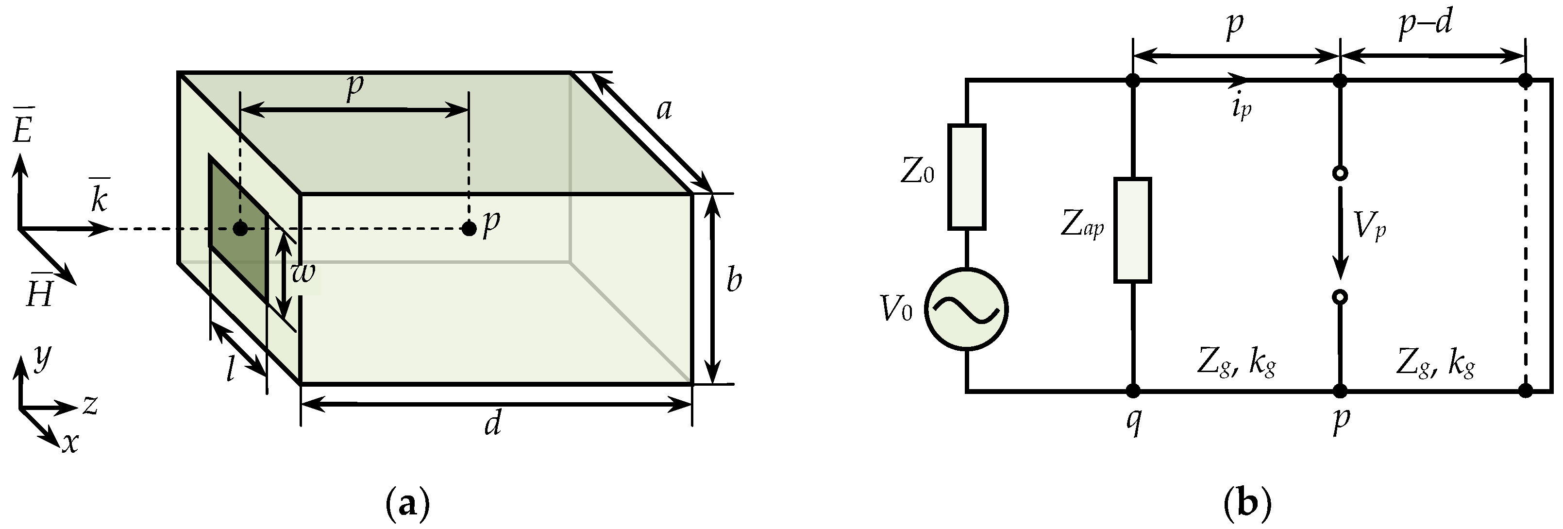
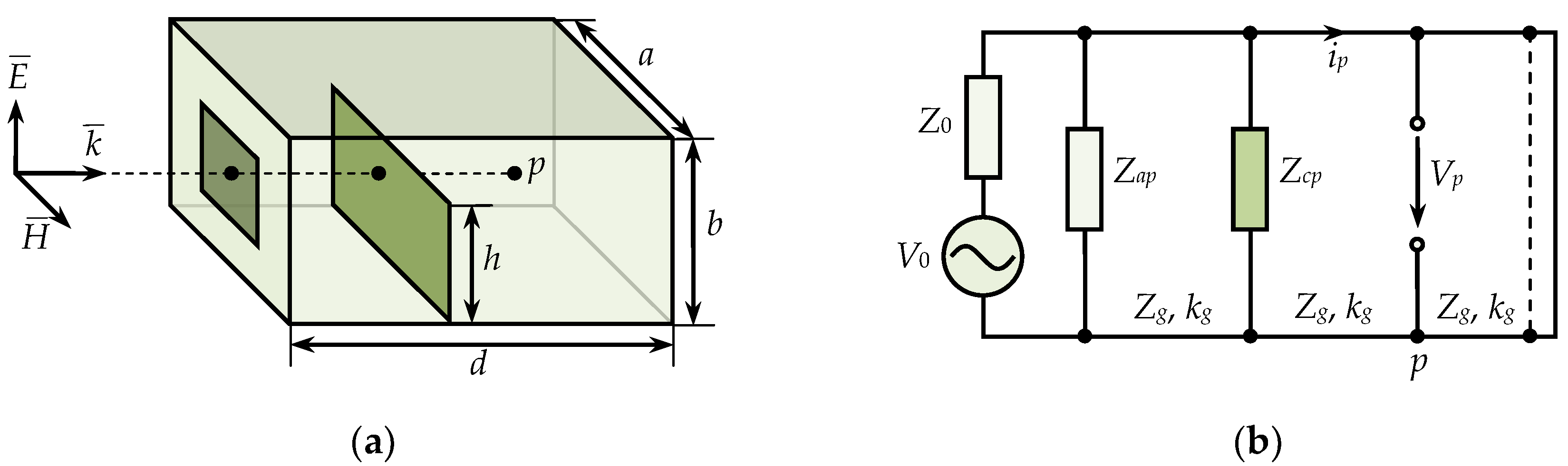
2.1. Formulation of Equivalent Circuit Model

According to [20], the rectangular enclosure with a volume of a × b × d m3 and a rectangular aperture (with an area of w × l m2) in the front wall (Figure 1a) are replaced by the equivalent circuit, shown in Figure 1b. In this circuit, a plane wave with frequency f, exciting the enclosure, is represented by a voltage source V0 and electrical resistance Z0 equal to the free-space impedance (120π Ω). This representation assumes that the plane wave is incident normal to the enclosure front wall, and the E-field vector is perpendicular to the length l of the aperture, giving a worst-case SE. The enclosure is replaced by segments of a rectangular waveguide with characteristic impedance Zg and propagation constant kg. The front wall with the aperture is represented by the Zap impedance. To calculate the SE, the equivalent circuit is transformed with respect to the observation point p, using Thevenin’s theorem and the transmission line theory. As a result, the SE values are determined from the current ip or voltage Vp in the equivalent circuit obtained after the transformation. Next, let us look at the SE calculation procedure using the model from [20] in more detail.
According to [20], in the first calculation step, the Zap impedance of the enclosure front wall is determined. It is assumed that the wall is replaced by two short-circuited segments of a coplanar stripline, each with a length of l/2 (i.e., half of the aperture width). The Zap value is calculated as the product of the correction factor l/a (where a is the width of the front wall) and the total input impedance of two segments connected in parallel:
Z a p = j 1 2 l a Z 0 s tan ( k 0 l 2 ) ,
where; j is the imaginary unit, k0 = 2π/λ is the free-space wavenumber, λ is the wavelength of the excitation source, and Z0s is the characteristic impedance of coplanar stripline, which can be calculated as:
Z 0 s = 120 π 2 [ ln ( 2 1 + 1 ( w e / b ) 2 4 1 1 ( w e / b ) 2 4 ) ] 1 ,
where; b is the height of the enclosure, and we is the effective height of the aperture, defined as:
w e = w 5 t 4 π ( 1 + ln 4 π w t ) ,
where; w is the height of the aperture, and t is the enclosure thickness.
Next, before transforming the equivalent circuit, the Zg and kg values are calculated for the rectangular waveguide segments replacing the enclosure. In [20], it is assumed that a dominant mode (TE10) is propagated in the enclosure, so Zg and kg are calculated as:
Z g = Z 0 / 1 ( λ 2 a ) 2 ,
k g = k 0 1 ( λ 2 a ) 2 .
Once Zap, Zg, and kg have been calculated, the procedure of the equivalent circuit transformation begins. First, the voltage source is transformed to point q in the circuit (see Figure 1b). For this purpose, V0 and Z0 are combined with Zap as:
V 1 = V 0 Z a p / ( Z 0 + Z a p ) ,
Z 1 = Z 0 Z a p / ( Z 0 + Z a p ) .
As a result of (4) and (5), the equivalent circuit takes the form shown in Figure 2a. The resulting excitation source is further transformed from point q to the observation point p. This gives the values of voltage V2 and impedance Z2. At the same time, the load impedance Z3 of the equivalent circuit is calculated, which is the input impedance of the short-circuited segment of the waveguide behind the observation point p. The following equations are used to calculate V2, Z2, and Z3 in [20]:
V 2 = V 1 cos ( k g p ) + j ( Z 1 / Z g ) sin ( k g p ) ,
Z 2 = Z 1 + j Z g tan ( k g p ) 1 1 + j ( Z 1 / Z g ) tan ( k g p ) ,
Z 3 = j Z g tan [ k g ( d p ) ] ,
where; d is the depth of the enclosure.
After calculating (6)–(8), the equivalent circuit takes the form shown in Figure 2b. In this circuit, it is easy to find the Vp and ip values needed to calculate the electrical and magnetic SE, respectively. For example, Vp can be calculated as:
V p = V 2 Z 3 Z 2 + Z 3 .
The electric SE at the observation point p is then defined as:
SE = 20 log 10 | 2 V p V 0 | .
In its original form, as described in [20], the analytical model, based on equivalent circuits, has a number of limitations. First, the shielding enclosure contains only one aperture with a rectangular shape and a central position on the front wall. Second, the SE evaluation technique does not take into account the resonances corresponding to higher-order modes (TEmn and TMmn) excited in the enclosure. Third, the equivalent circuit from Figure 1b does not take into account the internal filling of the enclosure or the aperture. There are other limitations, such as those imposed on the polarization and incidence angle of the plane wave exciting the enclosure due to its representation by a voltage source. However, a number of modifications to the model from [20] are known to overcome most of these limitations. We will look at some of them below.

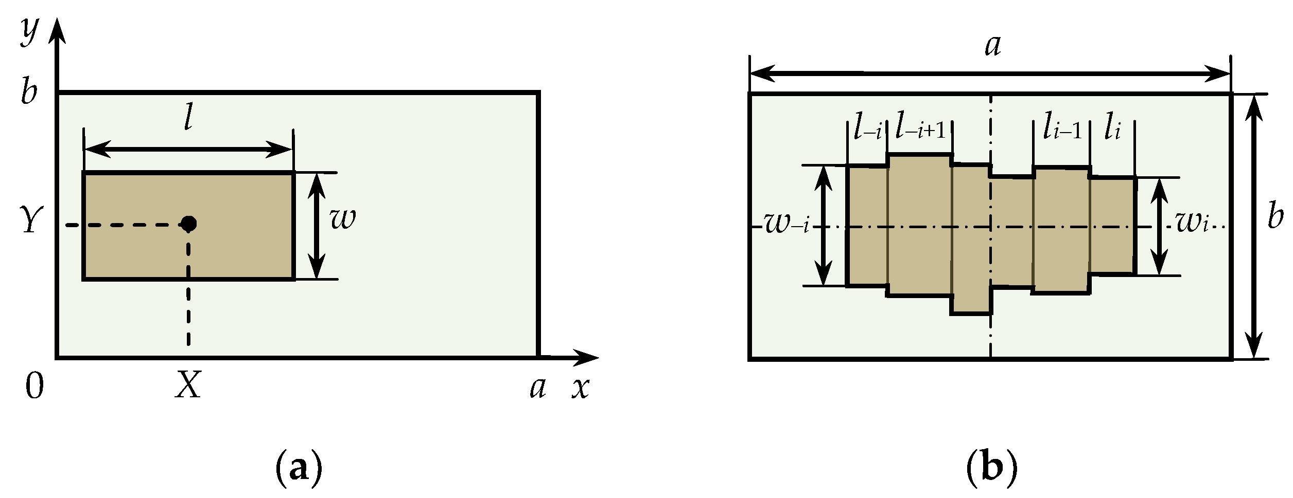
2.2. Modifications of Aperture Representation

Several modified models have been proposed in [21,22,23] to evaluate the SE of an enclosure with arbitrarily positioned aperture. However, the simplest and most accurate model has been developed by the authors of [24]. According to this model, the value of Zap at an arbitrary location of the aperture on the frontal wall can be calculated as the product of (1) and the following factor:
C m n = sin ( m π X a ) cos ( n π Y b ) ,
where; m and n are the not-negative integers, defining the numbers of TEmn and TMmn modes, and X and Y are the coordinates of the aperture centre on the front wall (see Figure 3).
In [25], a modified analytical model for evaluating the SE of an enclosure with a circular aperture of radius r was proposed. The Zap value can be calculated using (1) or (11), but, first, the geometric dimensions of an equivalent rectangular aperture must be determined. The following equation is used for this purpose:
l = w = r π .
According to [26], the Zap value for an elliptical shape aperture can be calculated as the product of (1) and (11). However, the characteristic impedance Z0s in (1) must be replaced by:
Z 0 s = Z m Z e Z m + Z e ,
where;
Z m = 1 2 [ k g 2 S 3 π Z g + S j 2 π f μ 0 χ m ] 1 ,
Z e = 2 [ k g 4 b 2 S 3 π Z g + j 2 π f ε 0 b 2 S χ e ] 1 ,
where; S is the area of the elliptic aperture, ε0 and μ0 are the electric and magnetic constants, and χe and χm are the electric and magnetic polarizabilities of the aperture calculated from its dimensions and complete elliptic integrals of the first and second kind (for more details see [26]), respectively.
Based on equivalent circuits, the SE evaluation for an enclosure with an arbitrary-shaped aperture can also be realized. For this purpose, according to [27,28], Zap can be calculated from the results of full-wave numerical analysis. However, in [29], a fully analytical formulation for determining the Zap impedance for an arbitrary-shaped aperture has been proposed. Starting from the centre, the aperture is divided into several intervals (Figure 3b). Each of these intervals is replaced by a segment of a regular coplanar stripline with length li and width wi. The transmission line segments replacing the aperture edges are assumed to be short-circuited. First, the input impedance Zin i of these segments is calculated, similar to (8). The calculated values act as loads for the following segments of the coplanar stripline, for which the input impedance is again calculated as:
Z i n = Z 0 s i Z i n i 1 + j Z 0 s i tan ( k 0 l i ) Z 0 s i + j Z i n i tan ( k 0 l i ) .
The calculation by (14) continues until the two input impedances to the left and right of the aperture centre have been determined. Eventually, Zap is determined from the parallel connection of these two input impedances.
Real shielding enclosures of electronic equipment usually contain several apertures with different shapes and sizes. To take this into account in the analytical SE evaluation, the following procedure was proposed in [25]. First, using (1) or (11)–(14), Zap N values are calculated separately for each aperture located on the front wall. Next, the total impedance of the enclosure wall with a set of N apertures is defined as:
Z a p = N Z a p N .
This procedure is well suited to apertures separated from each other because it ignores the mutual coupling between the apertures. For the same reason, it cannot be used for enclosures with perforated walls where the apertures are quite close. One model for calculating the impedance of a perforated wall has been proposed in [30], but it does not take into account the thickness (t) of the enclosure wall. This drawback is deprived by the model from [31]. In accordance with it, when a plane wave is incident normally to the enclosure wall, the Zap values are calculated as:
Z a p = j Z 0 l a w a 2 a b [ 1 + ( 3 d h d v λ 16 π r 3 ) ] 1 2 10 4 5 t r ,
where; la and wa are the width and height of the aperture array (see Figure 4a), dh and dv are the horizontal and vertical distances between the centers of apertures, and r is the radius of a single aperture.
Unfortunately, (16) gives correct results only when the aperture array is positioned in the centre of the front wall and cannot be used if the apertures are staggered (as in Figure 4b). A modified model from [32] was proposed for such cases. To take into account the arbitrary position of the aperture array, Equation (16) is multiplied by the correction factor C, defined as:
C = x 0 x 0 + l a y 0 y 0 + w a cos ( π y b ) cos [ π ( y y 0 ) w a ] sin ( π x a ) sin [ π ( x x 0 ) l a ] d y d x X Y ,
where X, Y and x0, y0 are the coordinates of the centre and beginning (bottom left corner) of the array, respectively. The array of staggered apertures in [32] is considered as two separate arrays with doubled vertical distances dv between the apertures. In this case, Zap = Zarr 1 + Zarr 2, where Zarr 1 and Zarr 2 are the impedances of two separate arrays, which are calculated by multiplying (16) and (17).

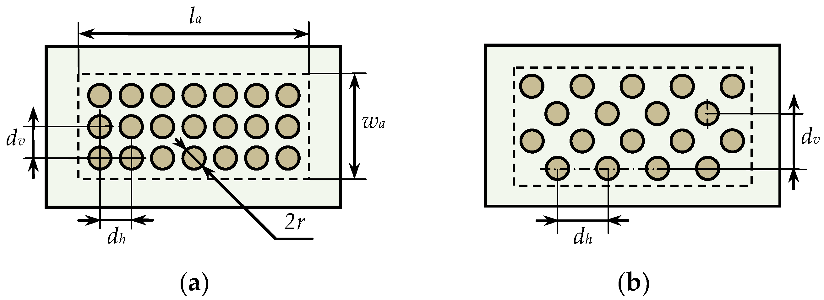
2.3. Internal Filling of Apertures

The apertures of real electronic equipment enclosures can be filled, e.g., with metal ventilation grilles, glass, rubber gaskets, etc. Such structures can affect the electromagnetic field inside the enclosure and resonances exciting in the apertures, thus they are worth considering in the SE evaluation. Several modifications of the equivalent circuit model have been developed to take into account the internal filling of the aperture. Thus, in [33], the authors proposed a formula for calculating the impedance Zap of a rectangular aperture populated with wire grid (Figure 5). The Zap value is defined as:
Z a p = l w a b [ 4 q w π D w 2 σ ψ I 0 ( ψ ) 2 I 1 ( ψ ) + j q w μ 0 f ln ( 1 1 exp [ π D w / q w ] ) ] ,
where; qw is the size of the grid cell, Dw is the wire diameter, ψ2 = j 0.5πμσ(Dw)2, σ and μ are the conductivity and absolute permeability of wires, and I0(ψ) and I1(ψ) are the modified Bessel functions of the first kind (zero and first order, respectively).
In [34], a formula for calculating Zap for an aperture filled with dielectric or magnetic material was proposed. As in [20], a front wall with the aperture is replaced by a coplanar stripline, but a material is added in the space between the line conductors. According to [34], Zap can be obtained as:
Z a p = j 1 2 l a 1 c C C tan ( π l λ C C ) ,
where; c is the speed of light in vacuum; C is the per-unit-length capacitance of the coplanar stripline, which only takes into account the relative permittivity εr of the material between the conductors; and is the same capacitance, but at εr = 1/μrr is the relative permeability of the material filling the aperture). In [35], another modification of the equivalent circuit model was proposed, which is suitable for an aperture populated with a liquid crystal display. However, this problem can also be solved using Formula (19). For this reason, we did not describe the model [35] in this section.

2.4. Higher Order Modes

The model from [20] assumes that only dominant mode TE10 propagates in the enclosure. However, if the electronic equipment enclosure is electrically small or is affected by broadband electromagnetic interference, higher-order modes TEmn or TMmn can be excited in the enclosure. In [23], a modification of the equivalent circuit model was proposed that takes into account higher-order modes in SE calculations. As in [20], the SE is determined from the current ip or voltage Vp values in the equivalent circuit, but these values are calculated iteratively. First, the characteristic impedance Zg mn and the propagation constant kg mn are calculated, depending on the non-negative integers m and n that determine the numbers of modes excited in the enclosure. For TEmn modes, Zg mn and kg mn are calculated as:
Z g m n = Z 0 / 1 ( λ m 2 a ) 2 ( λ n 2 b ) 2 ,
k g m n = k 0 1 ( λ m 2 a ) 2 ( λ n 2 b ) 2 .
For TMmn modes, the kg mn value is also calculated using (21), and Zg m is defined as:
Z g m n = Z 0 1 ( λ m 2 a ) 2 ( λ n 2 b ) 2 .
At the fixed values of Zg mn and kg mn, the transformation of the equivalent circuit is performed using expressions (4)–(8). Using (9), the voltage Vp mn for the current mode type and number is calculated and written to the counter. Then, the m and n indexes are changed, and the calculation is repeated again. As a result, based on the principle of superposition, voltages V p m n T E and V p m n T M are calculated, correspondingly, to TEmn and TMmn modes. The Vp value used to calculate the SE is then defined as:
V p = ( V p m n T E ) 2 + ( V p m n T M ) 2 .
Note that another approach for taking into account higher-order modes was proposed in [24]. However, the procedure of equivalent circuit transformation used in this approach is very different from the model [20], which makes it difficult to use this procedure in the generalized algorithm of SE evaluation.

2.5. Cylindrical Shaped Enclosure

Enclosures of electronic equipment elements can have not only a rectangular shape, but also a cylindrical one. Accordingly, a modified analytical model was proposed in [36] to evaluate the SE of such enclosures. It assumes that the aperture is located at the base of the cylindrical enclosure (see Figure 6), and SE is calculated using the same equivalent circuit as in [20].
To take into account the cylindrical shape of the enclosure, expressions for calculating the characteristic impedance and propagation constant in [36] are replaced by:
Z g m n = Z 0 / 1 ( λ / λ c m n ) 2 ,
k g m n = k 0 1 ( λ / λ c m n ) 2 ,
where; λc mn is the cut-off wavelength for the mode with indexes m and n, which can be calculated as [37]:
λ c m n = 2 π R / ξ m n ,
where; R is the enclosure radius, ξmn is the n-th root of equations Jmmn) = 0 (for TEmn modes), and Jmmn) = 0 (for TMmn modes), where Jmmn) is the Bessel function of order m, and Jmmn) is the first derivative of this function.

2.6. Internal Filling of Enclosures

Internal fillings, such as printed circuit boards, electronic components, cable assemblies, etc., can have a significant effect on the shielding and resonance performances of the enclosure. Several modifications of the equivalent circuit model have been developed to analyze filled enclosures. For example, in [38], a model was proposed to evaluate the SE of a rectangular enclosure populated with dielectric plates replacing the dielectric layers of printed circuit boards. In this equivalent circuit, the enclosure is represented as a set of rectangular waveguide sections with the same dimensions, but different dielectric properties of the materials filling their cross-sections (see Figure 7).
In waveguide sections populated with a dielectric, the characteristic impedance and propagation constant are calculated as:
Z g = Z 0 ε ^ r 1 (   λ   2 a ) 2 ,
k g = 2 π   λ   1 (   λ   2 a ) 2 ,
where; ε ^ r = ε’ – jε’’ is the complex relative permittivity of this dielectric, and   λ   = λ / ε ^ r .
A similar approach was used in [39] to analyze the SE of cylindrical enclosures filled with dielectrics. To calculate Zg and kg, the same expressions, (27)–(28), were used, but they had component 2a replaced by λc mn, calculated using (26). Another modification of the model from [20] is proposed in [40], in which the value of ε ^ r in (27)–(28) is replaced by the effective relative permittivity εeff. This version allows one to calculate the SE of an enclosure with dielectric structures of an arbitrary shape (but only when the TE10 dominant mode is excited).
In [41], the authors proposed a model to evaluate the SE of a rectangular enclosure filled with conductive posts, which can be used to approximate dipole antennas, wires, cable assemblies, etc. In the equivalent circuit, the post is replaced by a T-section formed by impedances jx1 and jx2 (see Figure 8).
The values of jx1 and jx2 are calculated as:
x 2 = ( a / λ g ) ( 2 π r 0 a ) 2 ( 1 + F 1 ) 1 ,
x 1 = ( a 2 λ g ) ( S F 0 F 0 ) x 2 2 ,
where; r0 is the radius of the post, λ g = λ / 1 ( λ / 2 a ) 2 is the wavelength in the waveguide, and the expressions for calculating F1, S , F , and F are not given in this paper to save space and to preserve narrative integrity.
In [42], the model was developed to evaluate the SE of an enclosure filled with conductive plates. This model can be used to approximate the conductive layers of printed circuit boards. The plate is considered as a capacitive waveguide diaphragm that fills the entire width of the enclosure (Figure 9a). In the equivalent circuit, the plate is replaced by the impedance Zcp (see Figure 9b), which is defined as:
Z c p = j B 1 ,
where; B is the susceptance of a capacitive diaphragm.
Several expressions for calculating the B values, depending on the plate height h, are given in [42]. For example, if the plate and enclosure heights are close (i.e., hb), B can be calculated as:
B = 4 b λ g Z 0 { π h 2 b + 1 6 ( π h 2 b ) 2 + 3 2 ( b λ g ) 2 ( π h 2 b ) 4 } .
However, the model from [42] has some limitations. For example, the plate is considered to be electrically connected to the enclosure and also always fills its entire width. The model proposed in [43] does not have these limitations. However, it uses numerical integration and Green’s functions to calculate the Zgp value, which makes it difficult to implement and use in engineering problems.

2.7. Summary

This review shows that most analytical models for evaluating the SE of electronic equipment enclosures are based on the same approach, i.e., they use equivalent circuits. With this in mind, these analytical models can easily be combined in calculating the SE of different shielding structures. Moreover, all these models can be combined into a generalized algorithm, since the equivalent circuits replacing the enclosures are transformed according to a strict step-by-step procedure based on well established principles of transmission line and circuit theories.

3. Generalized Algorithm
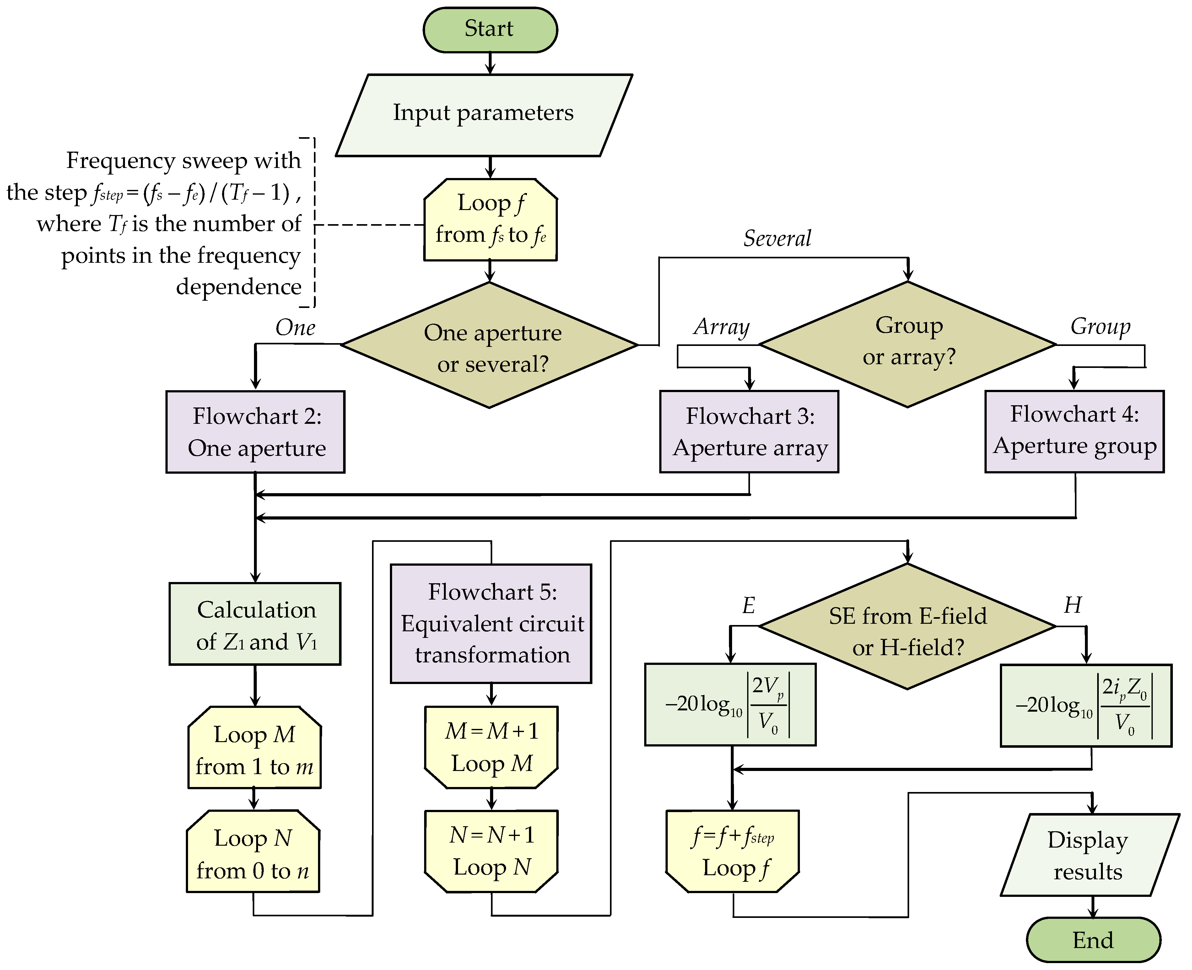
Here, we present a generalized algorithm for evaluating the SE of electronic equipment enclosures. For convenience, the algorithm is divided into separate functional parts, described below, in the form of flowcharts.

3.1. Main Flowchart

The main flowchart of the developed generalized algorithm is shown in Figure 10. SE calculations start with setting the excitation source parameters, the observation point position, as well as the characteristics of the enclosure, its apertures, and the inhomogeneities that fill the enclosure or apertures. The parameters are fed to the f loop input, which performs frequency sweeping from fs to fe. First of all, the expression for calculating Zap impedance is selected within the f loop. In addition, the Zap values can be calculated for a single aperture, an array, or a group of apertures. This is performed using flowcharts that can be found in the next section. Then, based on the calculated Zap value and Thevenin’s theorem, the values of voltage V1 and impedance Z1 are calculated using Equations (4) and (5). To take into account the higher-order modes excited in the enclosure, all subsequent transformations of the equivalent circuit are performed inside the M and N loops. Based on the results of these loops, we calculate the voltage Vp or current ip at the observation point. These values are then used to determine the electric and magnetic SE. When the f loop is complete, the SE values are output as a frequency dependence.

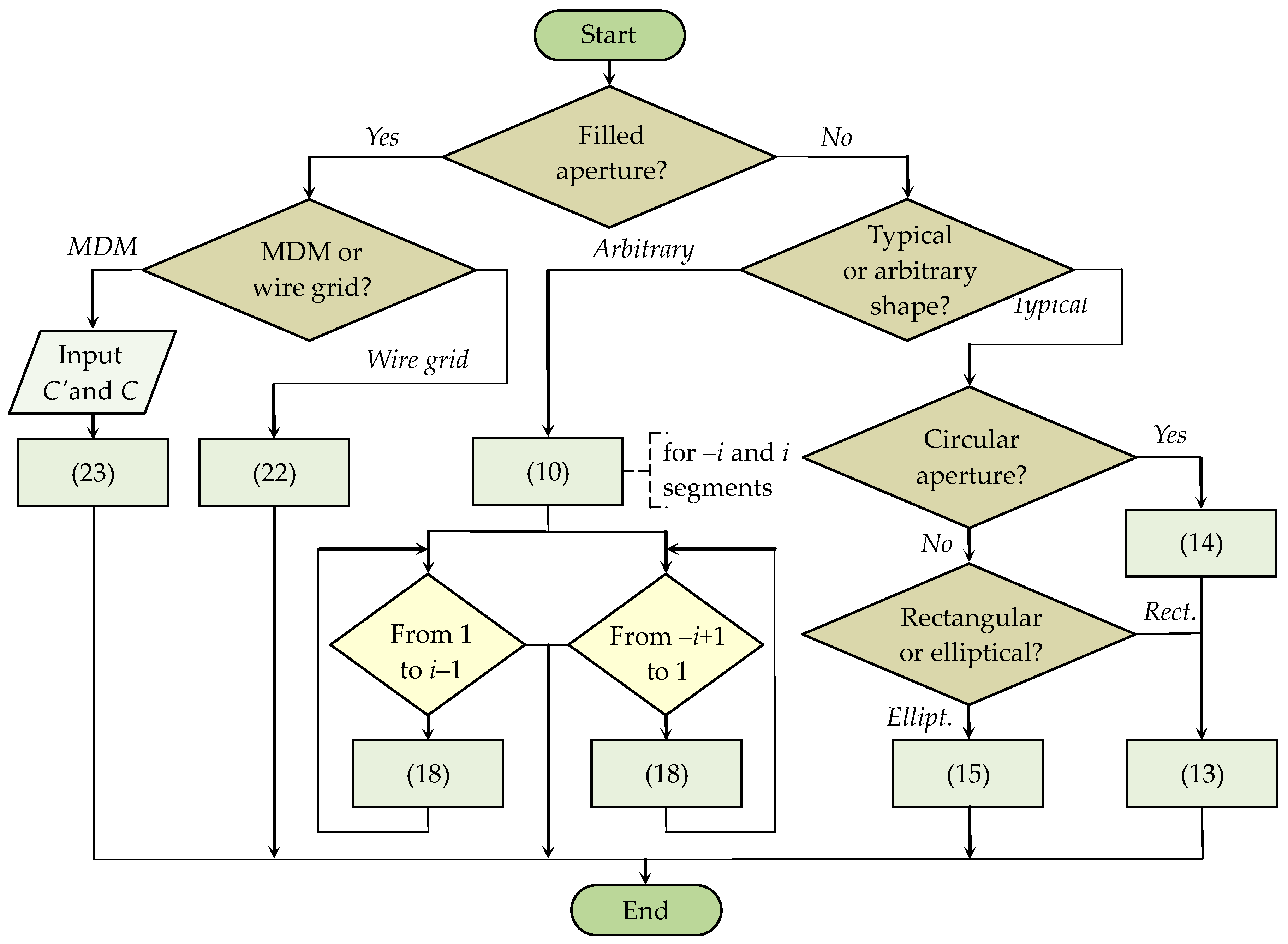
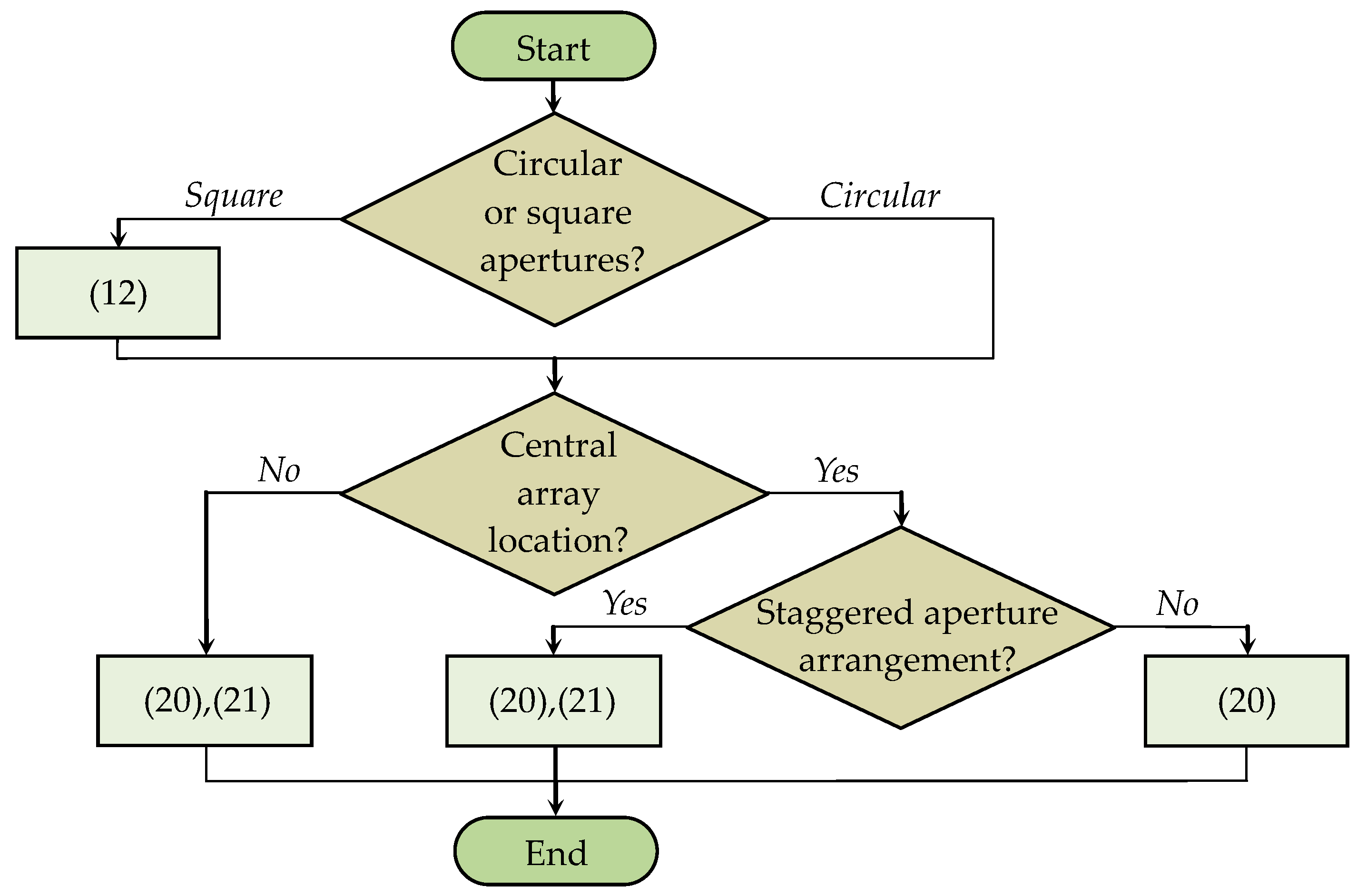
3.2. Algorithms for Calculating Aperture Impedance

In the main flowchart, the calculation of the Zap impedance for an enclosure wall with a single aperture follows the algorithm shown in Figure 11. The choice of analytical expression is made, depending on the shape and internal filling of the aperture. In particular, the algorithm takes into account the filling of the aperture with dielectric, magnetic, or magnetodielectric (MDM) materials, as well as wire grids. It also provides a procedure for calculating Zap for an arbitrarily shaped aperture, in accordance with the model from [29].
The expression for calculating the Zap impedance of the aperture array (i.e., perforated wall) is chosen based on the flowchart from Figure 12. When the aperture array is located outside the centre of the enclosure front wall, and when the apertures are staggered, the model from [32] is used to calculate Zap. This algorithm also allows Zap to be calculated for arrays of round or square apertures, which are implemented by expression (12) from [25].
Figure 13 illustrates a flowchart of the algorithm for selecting an analytical expression to calculate the Zap impedance for an enclosure wall with a group of apertures. If the enclosure wall contains an ordered group of identical circular or square apertures, then Zap is calculated according to [32]. In other cases, the expression for calculating Zap is chosen according to the algorithm from Figure 11.

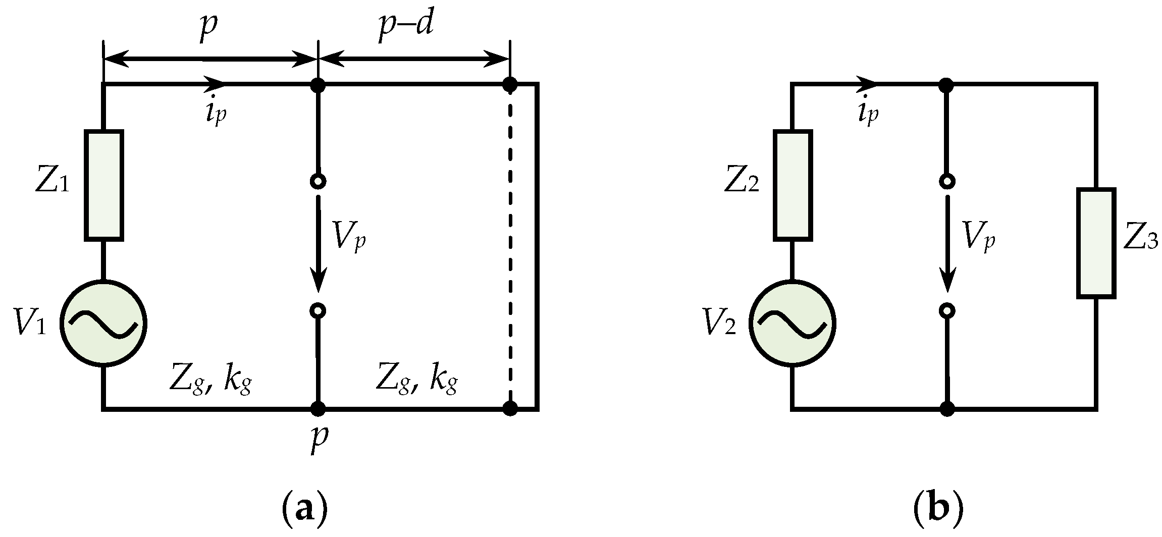
3.3. Algorithms for Equivalent Circuit Transformation

In the generalized algorithm, the transformation of equivalent circuits is carried out according to the flowchart shown in Figure 14. It provides four options for transforming the equivalent circuit, depending on the shape and internal filling of the enclosure. Thus, for empty enclosures, the first transformation step calculates the values of Zg mn and kg mn. The subsequent calculations are carried out in full accordance with the analytical model from [20]. For internally-filled enclosures, transformation of equivalent circuits is performed in accordance with the flowcharts shown in Figure 15 and Figure 16.
Figure 15 shows the algorithm used to transform an equivalent circuit for a filled rectangular enclosure. It starts by processing vector D containing all the dx points that define the positions of enclosure content. First, the “Sort (D)” block sorts points dx in ascending order (from 0 to d). The algorithm then determines the size (xmax) of vector D, and the number of the element xd corresponding to the observation point p. Next, for each point dx in the range x = 1, 2, …, xd − 1, the algorithm sequentially calculates filling parameters and intermediate values of voltages Vx and impedances Zx. When x = xd, the transformation for the left-hand side of the equivalent circuit ends. The last values of Vx and Zx are stored in the VL and ZL variables, and the algorithm proceeds to calculate the load impedance. The right-hand side of the circuit is transformed in reverse order from xmax to xd + 1. In each segment from d to p, intermediate values of Zx are calculated. The final load impedance ZR is determined when x = xd + 1. The values of VL, ZL, and ZR from the algorithm are then used to calculate Vp and ip.
Figure 16 presents a flowchart of the algorithm for transforming an equivalent circuit of filled cylindrical enclosure. It operates in a similar way to the algorithm in Figure 15, but the calculation does not take into account the conductive structures that fill the enclosure.

4. Algorithm Validation

Here, we present and discuss the validation results for the generalized algorithm we proposed for evaluating the SE.

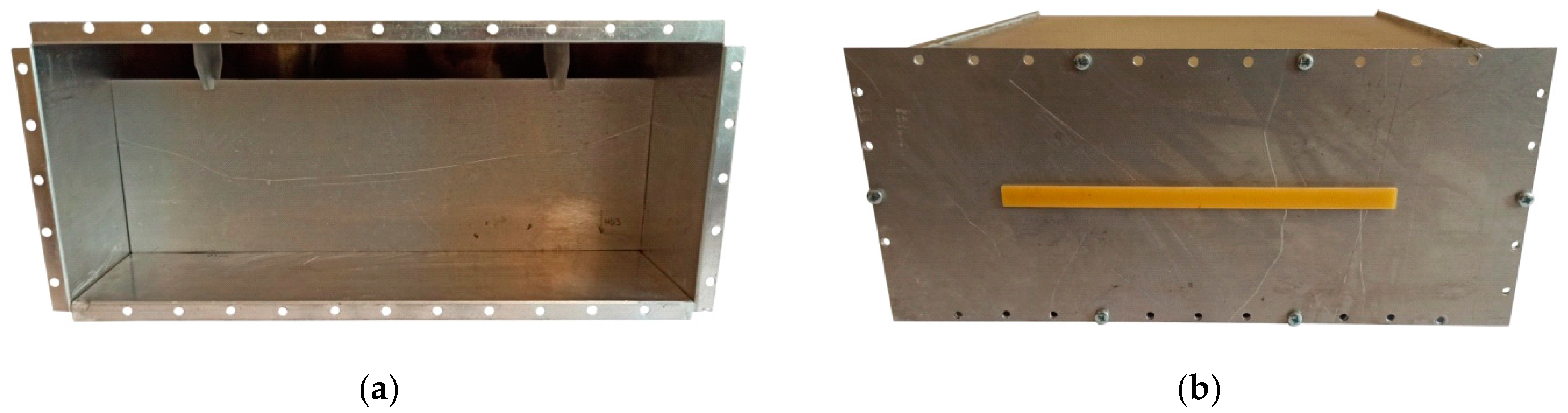
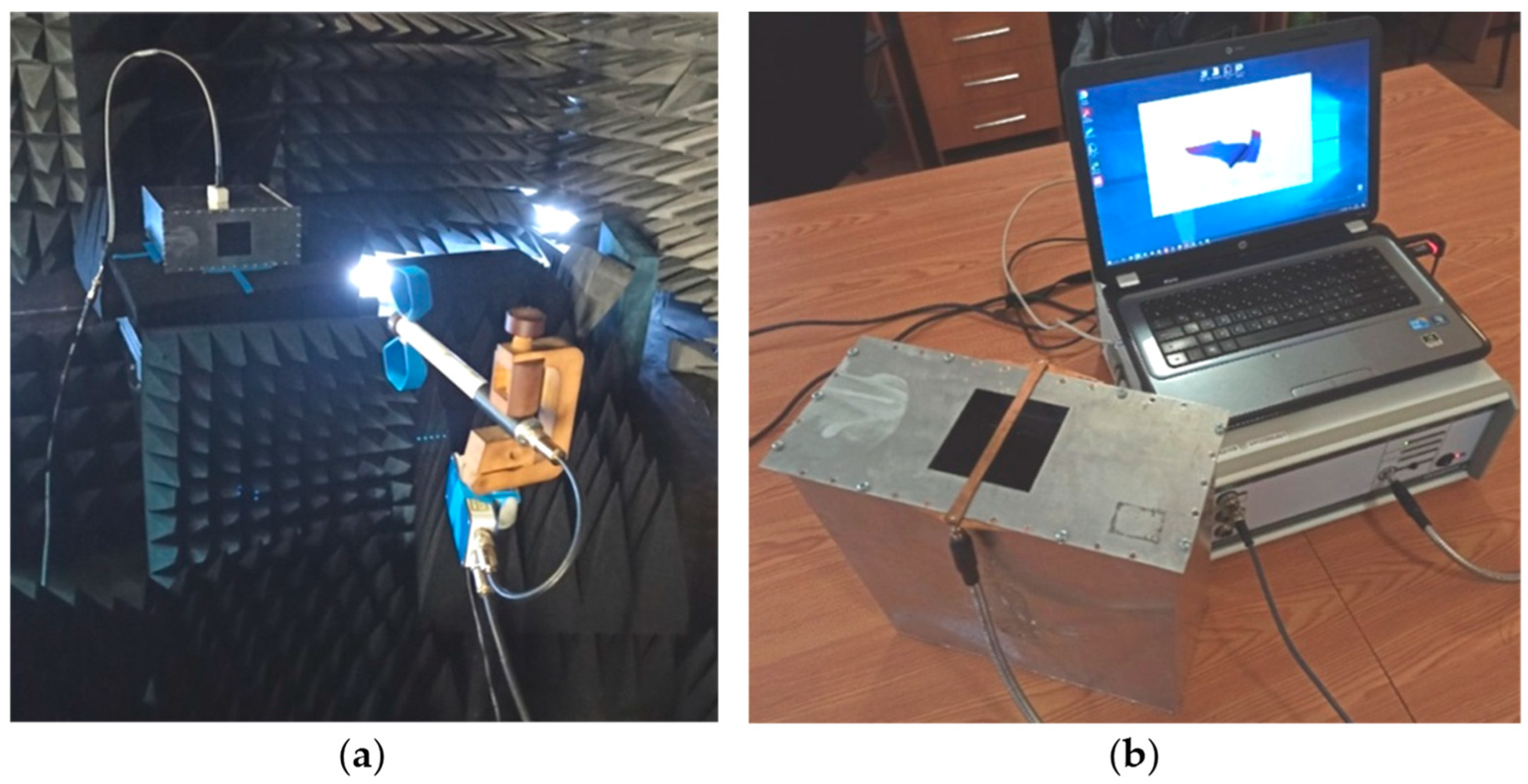
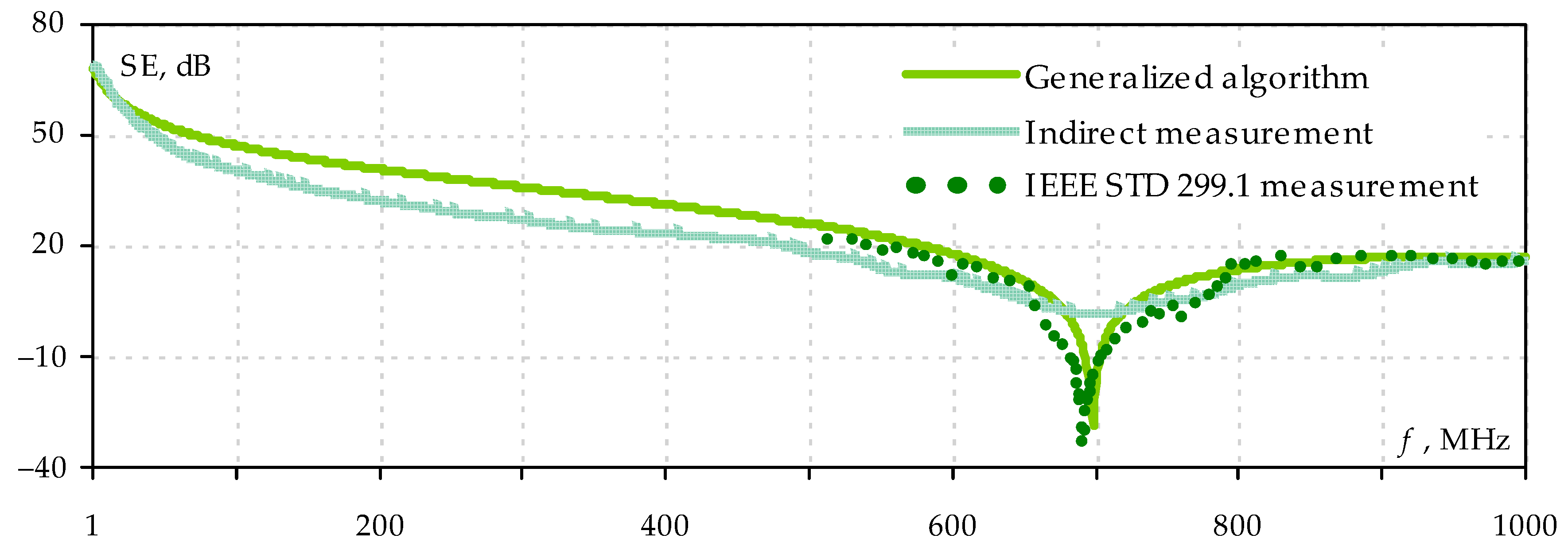
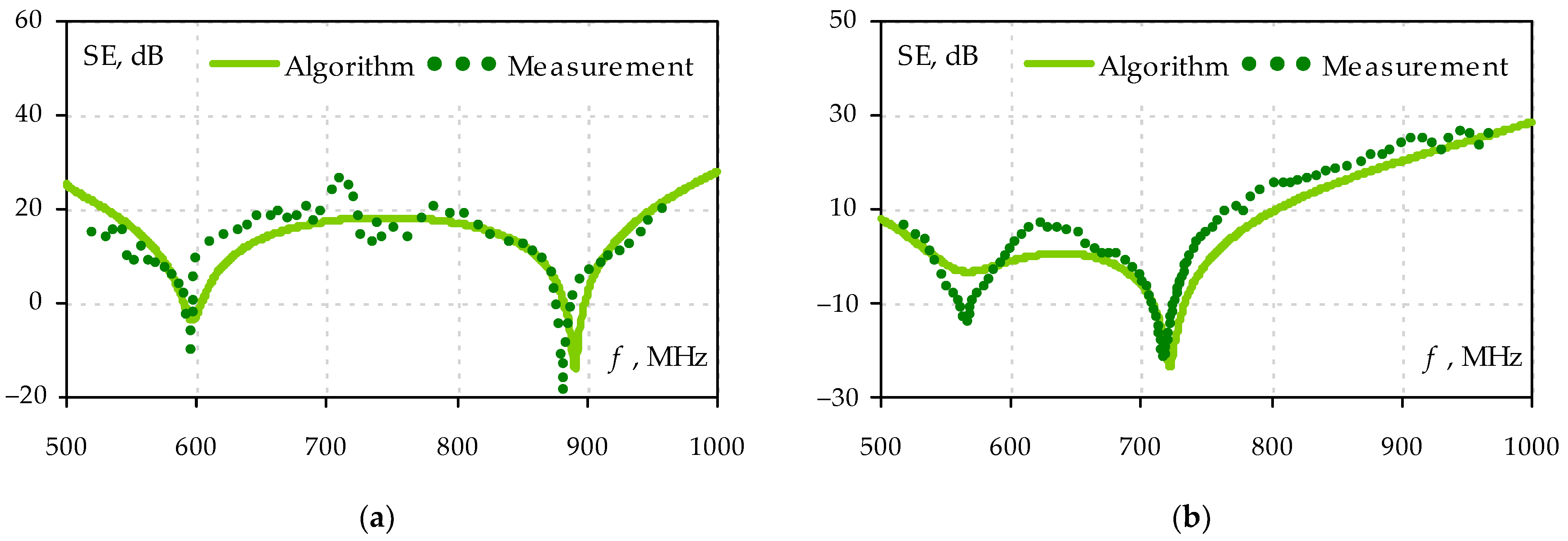
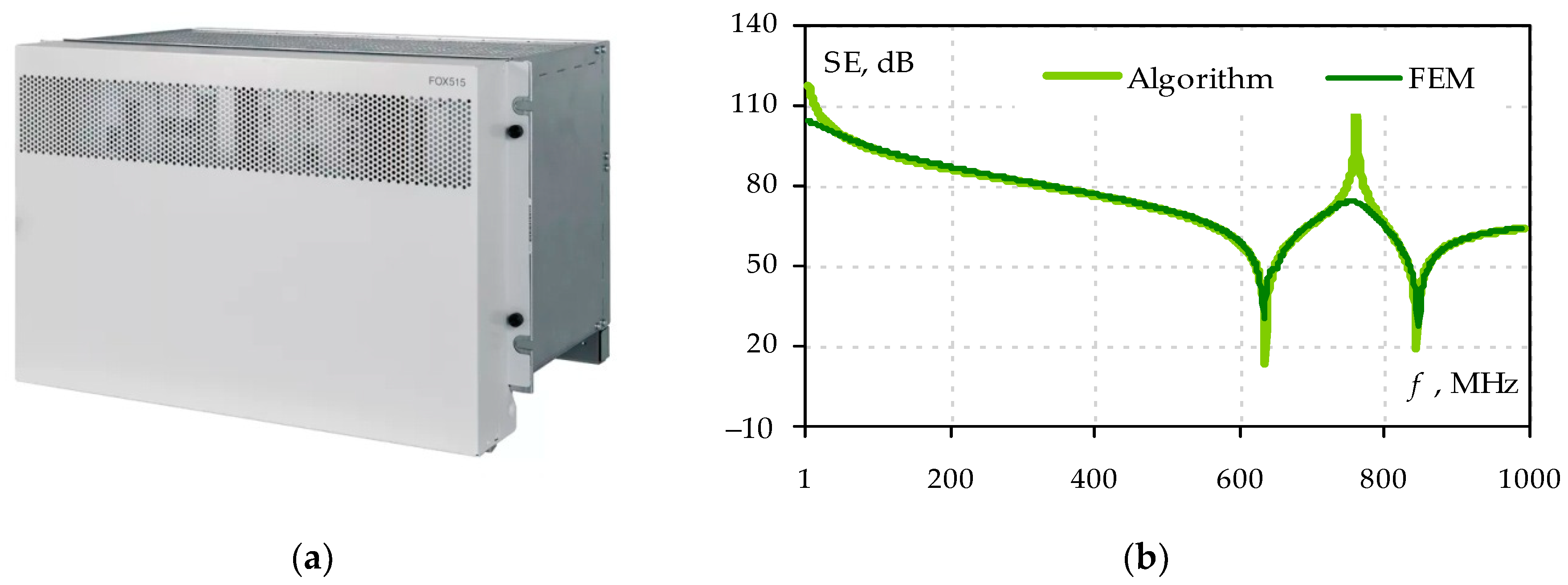
4.1. Validation by Measurement

First of all, validation of the developed algorithm was carried out by means of measurement. The SE frequency dependencies were calculated analytically and measured for an enclosure with dimensions a = d = 300 mm and b = 120 mm, taken from IEEE STD 1597.2 standard. A total of three cases were considered. In case 1, the enclosure was empty, and, in its front wall, there was a squared aperture with dimensions w = l = 80 mm (Figure 17). In case 2, the aperture was the same, but the enclosure was filled with a 100 mm high conductive plate, located at a distance of 75 mm from the front wall (Figure 18a). In case 3, the enclosure was empty again, and, in its front wall, there was a slot with w = 4 mm and l = 190 mm, which was filled with a dielectric with εr ≈ 3.3. In all cases, the SE was determined relative to the E-field at the observation point located in the centre of the enclosure, i.e., at p = 150 mm.
To measure the SE, we used a test setup that complies with the IEEE STD 299.1 standard. All measurements were carried out in a radio frequency anechoic chamber (Figure 19a). The SE values were determined from the transmission coefficient modules |S21| between the two antennas, using the following equation:
SE = 20 log 10 | S 21 0 | | S 21 | ,
where; index “0” denotes the values of |S21| measured in the absence of the enclosure.
The first antenna used in the test setup was an active Rusintell AI dipole with a maximum measurement error of 2 dB, which can only be used as a receiver. The dipole was placed outside of the enclosure and was vertically polarized. The dipole arms were oriented perpendicular to the wide wall of the enclosure, so that the maximum of the antenna pattern was directed towards the aperture. We did not place the receiving dipole antenna inside the enclosure, as it is quite large and could affect the field in the enclosure, i.e., shift the resonant frequencies, leading to incorrect SE results. The second antenna, which was used as a transmitter, was in the form of a small-sized quarter-wave monopole with a length of 25 mm and was placed in the center of the enclosure. Although IEEE STD 299.1 implies that the transmitting antenna must be outside the enclosure, the approach we have taken is consistent with the reciprocity principle of scattering and radiation problems and allows us to determine the SE quite accurately. The distance between two antennas was 1.5 m in all cases of |S21| measurement, including those where there was no enclosure. A Rohde & Schwarz (Munich, Germany) ZNL20 vector network analyzer, with less than 1 dB error, was used to obtain |S21| values. The test setup was used, starting from 500 MHz, due to the limited frequency range of the receiving dipole antenna.
For the enclosure from case 1 (with a squared aperture), the SE was also obtained by indirect measurement using the methodology proposed in [44]. For this purpose, a stripline with a 50 Ω impedance and a microwave resistor as a load was used (Figure 19b). The SE values were calculated, according to [44], based on the frequency dependence of the reflection coefficient modulus |S11| of this stripline when it is placed over the aperture of the shielding enclosure. The values of |S11| were determined with a Micran (Tomsk, Russia) R2M series scalar network analyzer, having less than 1.5 dB measurement error.
In order to calculate SE analytically, the separate parts of the proposed algorithm were implemented in GNU Octave. According to the algorithm, in case 1, Zap was determined, using Flowchart 2, based on Equation (13) at X = a/2 and Y = b/2. The equivalent circuit transformation was performed using Flowchart 5, taking into account only the TE10 mode. In case 2, Zap was defined, as in case 1, but the circuit transformation was performed according to Flowchart 6, calculating Zcp using (35). In case 3, the circuit was transformed, as in case 1, and Equation (23) was used to obtain Zap at ≈ 62.8 pF/m and C ≈ 31.9 pF/m.
When we performed indirect measurements and calculations using the proposed algorithm, the frequency dependencies of the SE were determined at a frequency resolution of about 1 MHz. For the measurement in the anechoic chamber, the frequency resolution was different for all three cases, but it was not less than 20 MHz. Additionally, in the resonance region, the number of frequency points was deliberately increased in order to determine the level of SE more accurately. To confirm the validity of the proposed algorithm, the average values of the absolute error modulus |Δ| were estimated. The calculation of |Δ| took into account all obtained SE values, including those in the resonance range. Frequency error (difference between resonances in SE frequency dependencies) was not taken into account. The |Δ| values were calculated as:
| Δ | = i = 1 T f | SE T ( f i ) SE A ( f i ) | T f
where; fi is some frequency point, indices T and A denote “true” (measured) and “observed” (calculated by the algorithm) values of the SE, and Tf is the number of points in the frequency dependence of “true” SE values.
Figure 20 shows the results of the analytical calculation and measurements for case 1 (for an empty enclosure with an 80 × 80 mm2 aperture). First of all, it can be seen that the enclosure SE is complex and can take positive and negative values when the frequency is changed. Negative SE occurs when coherent waves with the same phase are combined inside the enclosure, leading to cavity resonances. These resonances are a serious problem for electromagnetic compatibility of electronic equipment, as, at their frequencies, the shielding enclosure can amplify, rather than attenuate, interferences. Figure 20 also shows that the SE frequency dependencies obtained by different approaches are quite similar. The value of |Δ| between the results of the generalized algorithm and the indirect measurement was 5.7 dB. When comparing the results of the analytical calculation and the IEEE STD 299.1 measurement, a small difference (not more than 10 MHz) can be seen between the resonance frequencies. This difference may be caused by inaccuracy in the enclosure manufacture and the influence of the monopole antenna used in the measurement. Despite this, |Δ| = 5.2 dB.
Figure 21 illustrates the SE frequency dependencies for cases 2 and 3, obtained by measurements and the proposed algorithm. It can be seen that, in both cases, the measured and calculated dependencies are close. The |Δ| values were 5.6 dB and 4.2 dB for cases 2 and 3, respectively. Thus, the results shown in Figure 20 and Figure 21 confirm that the generalized algorithm can evaluate the SE with acceptable accuracy.

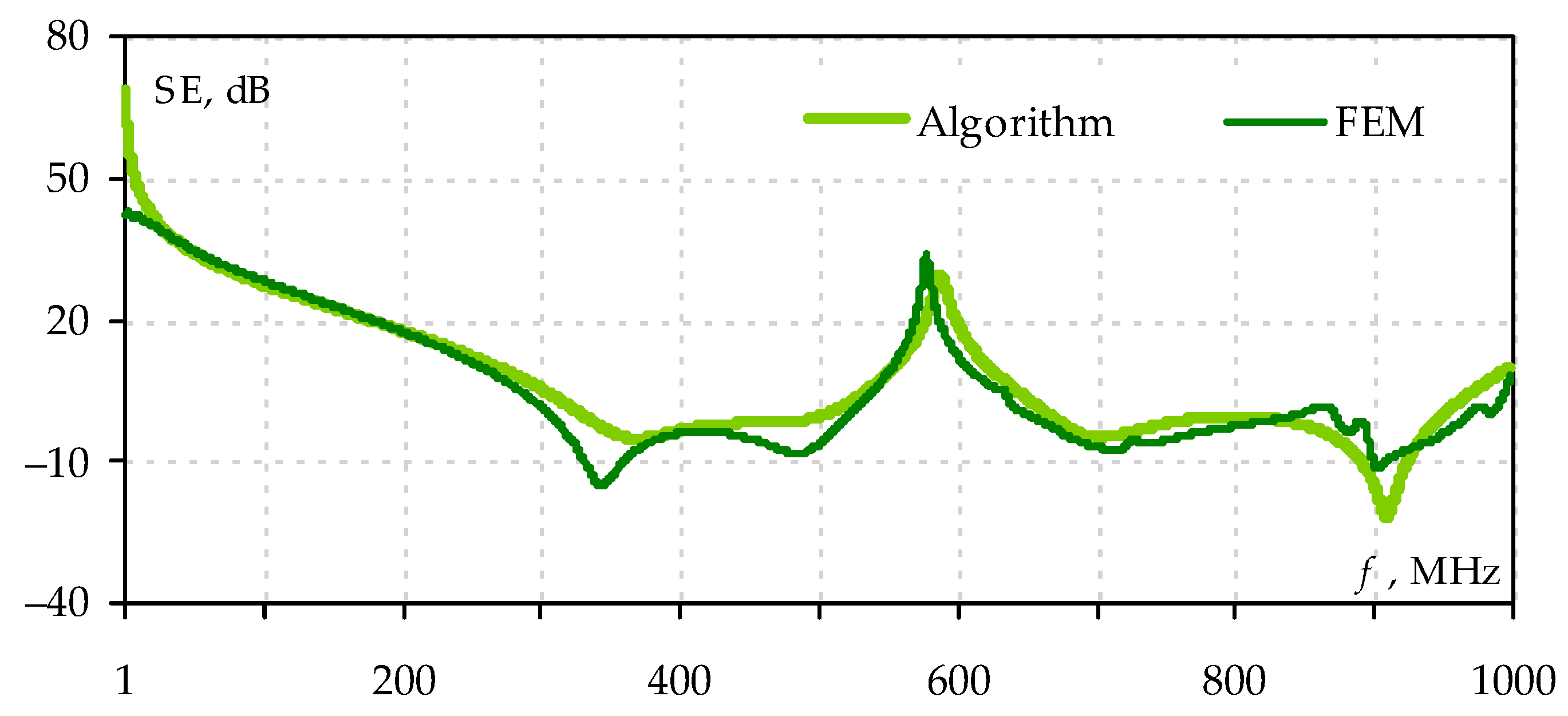
4.2. Validation by Numerical Analysis

Next, the generalized algorithm was validated using FEM-based numerical analysis. The COMSOL Multiphysics® (Stockholm, Sweden) RF Module was used for this purpose. In the FEM simulation, a perfect electrical conductor was used as the enclosure material. A hexagonal mesh with adaptive refinement was used to discretize the enclosures. The initial number of cells per wavelength was 45, and the mesh refinement percentage did not exceed 25% of the total number of elements at each step. The SE values were defined as:
SE = 20 log 10 | E 0 | | E | ,
where; E and E0 are the electric field strengths (intensities) at the observation point in the presence and absence of the enclosure, respectively. In all the cases considered below, the SE was calculated in the range from 1 MHz to 1 GHz with a resolution of just under 1 MHz, giving frequency dependencies consisting of 1000 points.
First, using FEM and the proposed algorithm, we calculated the SE for the enclosure of the Ethernet filter (Figure 22a). It has a volume of 440 × 42 × 197.5 mm3, a wall thickness of 1 mm, and it has 12 square apertures (16 × 16 mm2) on the front wall. The analysis was performed without the internal filling of the enclosure, and only the dominant mode excitation was taken into account in the analytical calculation (m = 1 and n = 0). When using the generalized algorithm, Zap was determined, according to Flowchart 4, based on the combination of Equations (14) and (20). The results are shown in Figure 22b. It can be seen that frequency dependencies of the SE, obtained by FEM and the proposed algorithm, are in good agreement, and |Δ| = 2.9 dB.
Next, we analyzed the enclosure of the ABB FOX 515 multiplexer (Figure 23a) with a volume of 445 × 270 × 278 mm3, a wall thickness of 1.5 mm, and an array of 108 × 15 circular staggered apertures (r = 1.5 mm) located at the top of the front wall. In the analytical calculation, the Zap was determined according to Flowchart 3 using Equations (20) and (21). The equivalent circuit transformation was performed, taking into account the excitation of higher-order modes in the enclosure (mixture of TE10, TE20 and TE30 modes). Figure 23b shows the SE frequency dependencies of the multiplexer enclosure calculated by FEM and the proposed algorithm. A small discrepancy can be seen between the frequency dependencies at low frequencies and in the region of 750 MHz. For the most part, however, the results are in good agreement, and the value of |Δ| is only 1.52 dB.
Finally, using FEM and the proposed algorithm, we calculated the frequency dependencies of the SE for a cylindrical enclosure with a circular aperture at R = r = 150 mm and d = 300 mm. Moreover, the enclosure under study was completely filled with dielectric material, with εr = 3.7. In the calculation by the proposed algorithm, Zap was determined using (13) and (14). The transformation of the equivalent circuit was performed according to Flowchart 7, and λc mn was determined at m = n = 1. Figure 24 illustrates that the results obtained by the generalized algorithm and FEM are in agreement. In this case, the value of |Δ| is 3.12 dB.

4.3. Computation Time Analysis

Table 1 presents the SE computation times for enclosures from Section 4.2 using the proposed generalized algorithm and FEM. Note that all calculations were performed on an outdated PC with a 6th-generation quad-core Intel Core i5 processor and 16 GB of RAM. It can be seen that the SE calculation by FEM takes considerably longer than that using the generalized algorithm based on equivalent circuits. In all cases, the time difference is more than 106 times.
Thus, the results of the algorithm validation prove that it has acceptable accuracy and low computation time. Consequently, using this algorithm in the early stages of designing electronic equipment, one can quickly evaluate the SE, which will significantly reduce the time for developing the final product.

5. Software Development

Based on the presented algorithm, we are currently developing software for the fast SE evaluation of electronic equipment enclosures. By the time of writing, our team has developed a prototype of this software. In this section, we briefly describe this prototype and its features.

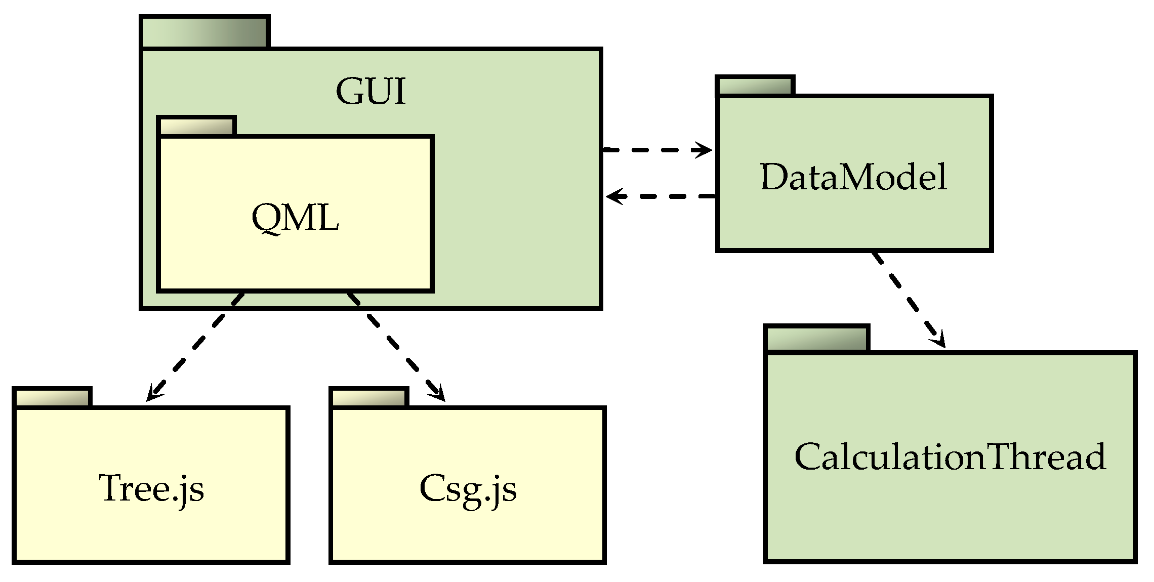
5.1. Programming Tools and Software Architecture

The C++ language and the Qt framework were chosen to develop the software prototype. The GUI of the prototype was developed using Qt Designer and the JavaScript-based Tree.js and Csg.js libraries, which have been adapted for QML (Qt’s built-in markup language). These libraries were used to create and visualise 3D-models of shielding enclosures.
Figure 25 presents the architecture of the software prototype in the form of a UML package diagram. The GUI is responsible for retrieving data from the DataModel and displaying it. The DataModel is an object model of the subject domain, which stores the input parameters for calculations, the data for displaying the SE, and the methods for operating with them. SE calculations are performed in the CalculationThread class, which implements the analytical expressions from Section 2. In addition, SE calculations are performed in a separate thread, which allows one to interact with the GUI at any time.

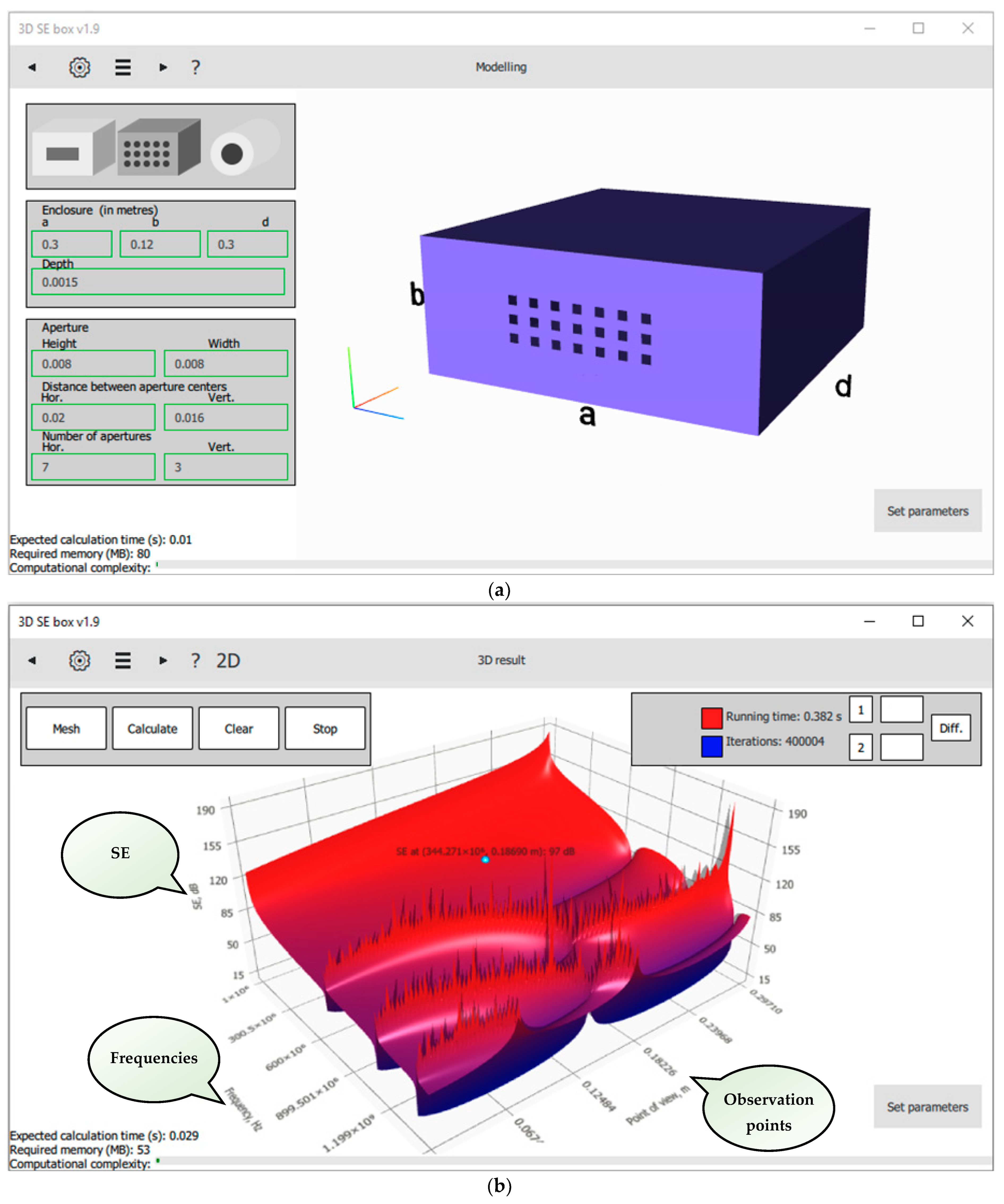
5.2. Software Feature

The software prototype developed so far implements only one part of the algorithm proposed in Section 3, which allows one to evaluate the SE of empty enclosures. However, some distinctive features and useful functionalities have been added to the prototype, and the authors feel that they should be presented in this article.
The main feature of the prototype is the ability to calculate and display a three-dimensional SE pattern, depending on the frequency of excitation source and the position of the observation point inside the enclosure. This feature makes it possible to identify areas where the SE has the worst values, which can be useful for selecting the optimum arrangement of electronic equipment parts within the shielding enclosure at the initial stage of design. An example of calculating a three-dimensional SE pattern in the prototype GUI is shown in Figure 26. Thus, Figure 26a illustrates the parameters and appearance of the enclosure under analysis. Figure 26b presents the SE pattern, depending on the frequency and the position of the observation point. The SEs are plotted along the vertical axis, and the frequency values (from 1 MHz to 2 GHz) and observation points along the enclosure (from 1 mm to 299 mm) are plotted along the other two axes.
The prototype also contains a functional for calculating the error between the SE frequency dependencies obtained in the software and in the external source. For this purpose, mechanisms for loading text files and data interpolation are implemented. To calculate the integrals in expression (17), the prototype uses the trapezoidal technique, together with Runge’s error estimation rule. The maximum error was set at 0.3%, which allowed us to reduce the computation time of Zap without losing the accuracy of the SE evaluation. The prototype also contains a functional for predicting the complexity of the SE computation, which operates based on data about the RAM of the PC running the software. This functional allows one to adjust the initial data or to abort an unreasonably long calculation before it begins.

6. Conclusions

This article has proposed a generalized algorithm, based on equivalent circuits, for evaluating the SEs of electronic equipment enclosures. We first reviewed and systematized most of the existing analytical models that use equivalent circuits in calculating the SE. After generalizing these models, we developed the SE evaluation algorithm and described it in the form of flowcharts. Next, using six different enclosures as examples, the algorithm was validated by two measurement methods and numerical analysis based on FEM. The validation results showed that the proposed algorithm allows one to calculate the SE more than 106 times faster than FEM. At the same time, it has an acceptable accuracy, since the average value of the absolute error modulus in all considered cases did not exceed 5.6 dB. The last part of this article presented a prototype of our software for analyzing shielding enclosures of electronic equipment, which we plan to develop further.
In conclusion, we prefer to note that, despite the good accuracy and low computation time, the algorithm proposed in this article has some disadvantages. The main one is its low variability due to the use of analytical models that cannot describe any arbitrary enclosure structure. For example, the algorithm cannot be used to analyze nested enclosures, unshielded cables penetrating the shield, enclosures with uneven or curved walls, etc. In contrast, almost any enclosure can be analyzed using numerical methods, although, as mentioned in the introduction, this requires significant computational costs. We believe that a new tool for a fast SE evaluation in the future could be a machine learning model. For this reason, some of our future research is expected to be devoted to developing and analyzing such a model. Another important disadvantage of the algorithm is that the enclosure is assumed to be perfectly conductive, i.e., penetration directly through the walls is ignored. This means that the algorithm is not well suited to the analysis of shields exposed to low-frequency and static H-fields.

Author Contributions

Conceptualization and methodology, M.E.K.; validation, A.A.I. and A.V.D.; software, A.A.I. and A.A.K.; writing—original draft preparation, A.A.I.; writing—review and editing, S.P.K. and T.R.G. All authors have read and agreed to the published version of the manuscript.

Funding

The review and algorithm development were financially supported by the Ministry of Science and Higher Education of the Russian Federation (Project FEWM-2022-0001). The measurement and software development were carried out at the expense of Russian Science Foundation grant 19-79-10162.

Data Availability Statement

The data presented in this study are available on request from the corresponding author. The data are not publicly available due to the funding organization policy.

Conflicts of Interest

The authors declare no conflict of interest.

References

  1. Ott, H.W. Electromagnetic Compatibility Engineering, 1st ed.; John Wiley & Sons, Inc.: Hoboken, NJ, USA, 2009. [Google Scholar]
  2. Kallambadi Sadashivappa, P.; Venkatachalam, R.; Pothu, R.; Boddula, R.; Banerjee, P.; Naik, R.; Radwan, A.B.; Al-Qahtani, N. Progressive review of functional nanomaterials-based polymer nanocomposites for efficient EMI shielding. J. Compos. Sci. 2023, 7, 77. [Google Scholar] [CrossRef]
  3. Schulz, R.B. Shielding theory and practice. IEEE Trans. Electromagn. Compat. 1988, 30, 187–201. [Google Scholar] [CrossRef]
  4. Ren, J.; Pan, Y.; Zhou, Z.; Zhang, T. Research on testing method for shielding effectiveness of irregular cavity based on field distribution characteristics. Electronics 2023, 12, 1035. [Google Scholar] [CrossRef]
  5. Basyigit, I.B.; Dogan, H.; Helhel, S. The effect of aperture shape, angle of incidence and polarization on shielding effectiveness of metallic enclosures. J. Microw. Power Electromagn. Energy 2019, 53, 115–127. [Google Scholar] [CrossRef]
  6. Azizi, H.; Tahar Belkacem, F.; Moussaoui, D.; Moulai, H.; Bendaoud, A.; Bensetti, M. Electromagnetic interference from shielding effectiveness of a rectangular enclosure with apertures—Circuital approach, FDTD and FIT modelling. J. Electromagn. Waves Appl. 2014, 28, 494–514. [Google Scholar] [CrossRef]
  7. Flintoft, I.D.; Bale, S.J.; Marvin, A.C.; Ye, M.; Dawson, J.F.; Wan, G.; Zhang, M.; Parker, S.L.; Robinson, M.P. Representative Contents Design for Shielding Enclosure Qualification From 2 to 20 GHz. IEEE Trans. Electromagn. Compat. 2018, 60, 173–181. [Google Scholar] [CrossRef] [Green Version]
  8. Kwon, J.H.; Hyoung, C.H.; Hwang, J.-H.; Park, H.H. Impact of absorbers on the shielding effectiveness of metallic rooms with apertures. Electronics 2021, 10, 237. [Google Scholar] [CrossRef]
  9. Rusiecki, A.; Aniserowicz, K.; Orlandi, A.; Duffy, A.P. Internal stirring: An approach to approximate evaluation of shielding effectiveness of small slotted enclosures. IET Sci. Meas. Technol. 2016, 10, 659–664. [Google Scholar] [CrossRef] [Green Version]
  10. Kubík, Z.; Skála, J. Shielding effectiveness measurement and simulation of small perforated shielding enclosure using FEM. In Proceedings of the 2015 IEEE 15th International Conference on Environment and Electrical Engineering, Rome, Italy, 10–13 June 2015; pp. 1983–1988. [Google Scholar]
  11. Jiao, C.; Li, L.; Cui, X.; Li, H. Subcell FDTD analysis of shielding effectiveness of a thin-walled enclosure with an aperture. IEEE Trans. Magn. 2006, 42, 1075–1078. [Google Scholar] [CrossRef]
  12. Attari, A.R.; Barkeshli, K.; Ndagijimana, F.; Dansou, J. Application of the transmission line matrix method to the calculation of the shielding effectiveness for metallic enclosures. In Proceedings of the IEEE Antennas and Propagation Society International Symposium, San Antonio, TX, USA, 16–21 June 2002; pp. 302–305. [Google Scholar]
  13. Celozzi, S.; Araneo, R.; Lovat, G. Electromagnetic Shielding; John Wiley & Sons, Inc.: Hoboken, NJ, USA, 2008. [Google Scholar]
  14. Hill, D.A.; Ma, M.T.; Ondrejka, A.R.; Riddle, B.F.; Crawford, M.L.; Johnk, R.T. Aperture excitation of electrically large, lossy cavities. IEEE Trans. Electromagn. Compat. 1994, 36, 169–178. [Google Scholar] [CrossRef]
  15. Jeong, I.H.; Lee, J.W.; Lee, Y.S.; Kwon, J.-H. Shielding effectiveness estimation in an electrically large cavity using power balance method and BLT equation. In Proceedings of the 2014 International Symposium on Electromagnetic Compatibility, Gothenburg, Sweden, 1–4 September 2014; pp. 444–447. [Google Scholar]
  16. Flintoft, I.D.; Marvin, A.C.; Funn, F.I.; Dawson, L.; Zhang, X.; Robinson, M.P.; Dawson, J.F. Evaluation of the diffusion equation for modeling reverberant electromagnetic fields. IEEE Trans. Electromagn. Compat. 2017, 59, 760–769. [Google Scholar] [CrossRef]
  17. Yan, J.; Dawson, J.; Marvin, A. Estimating reverberant electromagnetic fields in populated enclosures by using the diffusion model. In Proceedings of the 2018 IEEE Symposium on Electromagnetic Compatibility, Signal Integrity and Power Integrity, Long Beach, CA, USA, 30 July–3 August 2018; pp. 363–367. [Google Scholar]
  18. Solin, J.R. Formula for the field excited in a rectangular cavity with a small aperture. IEEE Trans. Electromagn. Compat. 2011, 53, 82–90. [Google Scholar] [CrossRef]
  19. Solin, J.R. Formula for the field excited in a rectangular cavity with an electrically large aperture. IEEE Trans. Electromagn. Compat. 2012, 54, 188–192. [Google Scholar] [CrossRef]
  20. Robinson, M.P.; Turner, J.D.; Thomas, D.W.P.; Dawson, J.F.; Ganley, M.D.; Marvin, A.C.; Porter, S.J.; Benson, T.M.; Christopoulos, C. Shielding effectiveness of a rectangular enclosure with a rectangular aperture. Electron. Lett. 1996, 32, 1559–1560. [Google Scholar] [CrossRef]
  21. Po’ad, F.A.; Jenu, M.Z.M.; Christopoulos, C.; Thomas, D.W.P. Analytical and experimental study of the shielding effectiveness of a metallic enclosure with off-centered apertures. In Proceedings of the 2006 17th International Zurich Symposium on Electromagnetic Compatibility, Singapore, 27 February–3 March 2006; pp. 618–621. [Google Scholar]
  22. Nie, B.L.; Du, P.A. An efficient and reliable circuit model for the shielding effectiveness prediction of an enclosure with an aperture. IEEE Trans. Electromagn. Compat. 2015, 57, 357–364. [Google Scholar] [CrossRef]
  23. Shi, D.; Shen, Y.; Gao, Y. 3 High-order Mode Transmission Line Model of Enclosure with Off-center Aperture. In Proceedings of the 2007 International Symposium on Electromagnetic Compatibility, Qingdao, China, 23–26 October 2007; pp. 361–364. [Google Scholar]
  24. Yin, M.C.; Liu, E.; Du, P.A. Improved circuit model for the prediction of the shielding effectiveness and resonances of an enclosure with apertures. IEEE Trans. Electromagn. Compat. 2016, 58, 448–456. [Google Scholar] [CrossRef]
  25. Robinson, M.P.; Benson, T.M.; Christopoulos, C.; Dawson, J.F.; Ganley, M.D.; Marvin, A.C.; Porter, S.J.; Thomas, D.W.P. Analytical formulation for the shielding effectiveness of enclosures with apertures. IEEE Trans. Electromagn. Compat. 1998, 40, 240–248. [Google Scholar] [CrossRef] [Green Version]
  26. Rabat, A.; Bonnet, P.; Ei Khamlichi Drissi, K.; Girard, S. Novel analytical formulation for shielding effectiveness calculation of lossy enclosures containing elliptical apertures. In Proceedings of the 2018 International Symposium on Electromagnetic Compatibility, Amsterdam, The Netherlands, 27–30 August 2018; pp. 735–739. [Google Scholar]
  27. Inbavalli, V.P.; Venkatesh, C.; Suresh Kumar, T.R. Calculation of shielding effectiveness of an enclosure with arbitrary shaped apertures using hybrid approach. In Proceedings of the 2018 15th International Conference on ElectroMagnetic Interference & Compatibility, Bengaluru, India, 13–16 November 2018; pp. 1–4. [Google Scholar]
  28. Hu, P.Y.; Sun, X.Y.; Chen, J. Hybrid model for estimating the shielding effectiveness of metallic enclosures with arbitrary apertures. IET Sci. Meas. Technol. 2020, 14, 462–470. [Google Scholar] [CrossRef]
  29. HongYi, L.; Su, D.; Yao, C.; ZiHua, Z. Analytically calculate shielding effectiveness of enclosure with horizontal curved edges aperture. Electron. Lett. 2017, 53, 1638–1640. [Google Scholar] [CrossRef]
  30. Dehkhoda, P.; Tavakoli, A.; Moini, R. An efficient shielding effectiveness calculation (A rectangular enclosure with numerous square apertures). In Proceedings of the 2007 IEEE International Symposium on Electromagnetic Compatibility, Honolulu, HI, USA, 9–13 July 2007; pp. 1–4. [Google Scholar]
  31. Nie, B.-L.; Du, P.-A.; Xiao, P. An improved circuital method for the prediction of shielding effectiveness of an enclosure with apertures excited by a plane wave. IEEE Trans. Electromagn. Compat. 2018, 60, 1376–1383. [Google Scholar] [CrossRef]
  32. Ivanov, A.A.; Komnatnov, M.E. Model for estimating the shielding effectiveness of an enclosure with a perforated wall. IOP Conf. Ser. Mater. Sci. Eng. 2020, 734, 012078. [Google Scholar] [CrossRef]
  33. Chen, L.; He, R.; Jiao, C.; Hu, Y. Shielding effectiveness analysis of a rectangular enclosure with wire mesh covering. IOP Conf. Ser. Mater. Sci. Eng. 2019, 569, 022035. [Google Scholar] [CrossRef]
  34. Ivanov, A.A.; Demakov, A.V.; Komnatnov, M.E.; Gazizov, T.R. Semi-analytical approach for calculating shielding effectiveness of an enclosure with a filled aperture. Electrica 2022, 22, 220–225. [Google Scholar] [CrossRef]
  35. Kim, S.; Park, D.; Lee, J. Shielding effectiveness of an enclosure with a dielectric-backed aperture using slotline method. In Proceedings of the 2007 International Symposium on Electromagnetic Compatibility, Qingdao, China, 23–26 October 2007; pp. 432–435. [Google Scholar]
  36. Wang, Y.; Zhao, X.; Chen, J.; Sun, X. The analysis of multi-mode cylindrical enclosure shielding effectiveness with apertures. In Proceedings of the 2010 International Conference on Computer, Mechatronics, Control and Electronic Engineering, Changchun, China, 24–26 August 2010; pp. 527–530. [Google Scholar]
  37. Collin, R.E. Field Theory of Guided Waves, 2nd ed.; IEEE Press: Piscataway, NJ, USA, 1990. [Google Scholar]
  38. Li, F.; Han, J.; Zhang, C. Study on the influence of PCB parameters on the shielding effectiveness of metal cavity with holes. In Proceedings of the 2019 IEEE 3rd Information Technology, Networking, Electronic and Automation Control Conference, Chengdu, China, 15–17 March 2019; pp. 383–387. [Google Scholar]
  39. Ivanov, A.A.; Komnatnov, M.E. Analytical model for estimating the shielding effectiveness of cylindrical connectors. IOP Conf. Ser. Mater. Sci. Eng. 2019, 560, 012020. [Google Scholar] [CrossRef]
  40. Ivanov, A.A.; Komnatnov, M.E. Analytical model of a shielding enclosure populated with arbitrary shaped dielectric obstacles. J. Phys. Conf. Ser. 2021, 1889, 022110. [Google Scholar] [CrossRef]
  41. Thomas, D.W.P.; Denton, A.; Konefal, T.; Benson, T.M.; Christopoulos, C.; Dawson, J.F.; Marvin, A.C.; Porter, J. Characterisation of the shielding effectiveness of loaded equipment enclosures. In Proceedings of the International Conference and Exhibition on Electromagnetic Compatibility, York, UK, 13–12 July 1999; pp. 89–94. [Google Scholar]
  42. Ivanov, A.A.; Komnatnov, M.E.; Gazizov, T.R. Analytical model for evaluating shielding effectiveness of an enclosure populated with conducting plates. IEEE Trans. Electromagn. Compat. 2020, 62, 2307–2310. [Google Scholar] [CrossRef]
  43. Thomas, D.W.P.; Denton, A.C.; Konefal, T.; Benson, T.; Christopoulos, C.; Dawson, J.F.; Marvin, A.; Porter, S.J.; Sewell, P. Model of the electromagnetic fields inside a cuboidal enclosure populated with conducting planes or printed circuit boards. IEEE Trans. Electromagn. Compat. 2001, 43, 161–169. [Google Scholar] [CrossRef]
  44. Shourvarzi, A.; Joodaki, M. Shielding effectiveness estimation of a metallic enclosure with an aperture using S-parameter analysis: Analytic validation and experiment. IEEE Trans. Electromagn. Compat. 2017, 59, 537–540. [Google Scholar] [CrossRef]
Figure 1. Rectangular enclosure with aperture excited by a plane wave (a), equivalent circuit for calculating SE (b).
Algorithms 16 00294 g001
Figure 2. Equivalent circuits after the first (a) and second (b) transformation steps.
Algorithms 16 00294 g002
Figure 3. Front wall with an aperture shifted to the left (a), arbitrarily shaped aperture replaced by a set of coplanar stripline segments (b).
Algorithms 16 00294 g003
Figure 4. Enclosure front wall perforated with circular apertures (a), array of staggered apertures (b).
Algorithms 16 00294 g004
Figure 5. The aperture populated with wire grid (a) and geometry of this wire grid (b).
Algorithms 16 00294 g005
Figure 6. Cylindrical enclosure with the aperture at the base.
Algorithms 16 00294 g006
Figure 7. Enclosure populated with dielectric plate (a), equivalent circuit for calculating SE (b).
Algorithms 16 00294 g007
Figure 8. Enclosure filled with a conductive post (a), equivalent circuit for calculating SE (b).
Algorithms 16 00294 g008
Figure 9. Enclosure filled with a conductive plate (a), equivalent circuit for calculating SE (b).
Algorithms 16 00294 g009
Figure 10. Main flowchart of the generalized algorithm for the SE evaluation.
Algorithms 16 00294 g010
Figure 11. Algorithm of Zap calculation for a single aperture (Flowchart 2).
Algorithms 16 00294 g011
Figure 12. Algorithm of Zap calculation for an aperture array or a perforated wall (Flowchart 3).
Algorithms 16 00294 g012
Figure 13. Algorithm of Zap calculation for a group of apertures (Flowchart 4).
Algorithms 16 00294 g013
Figure 14. Algorithm of equivalent circuit transformation (Flowchart 5).
Algorithms 16 00294 g014
Figure 15. Algorithm of equivalent circuit transformation for a rectangular enclosure with internal filling (Flowchart 6).
Algorithms 16 00294 g015
Figure 16. Algorithm of equivalent circuit transformation for a cylindrical enclosure with internal filling (Flowchart 7).
Algorithms 16 00294 g016
Figure 17. Empty enclosure with a squared aperture of 80 × 80 mm2.
Algorithms 16 00294 g017
Figure 18. Enclosure populated with conductive plate (a), enclosure with dielectric filled slot (b). In the left photo, the enclosure has no wall.
Algorithms 16 00294 g018
Figure 19. Test setups for measuring SE according to IEEE STD 299.1 (a) and using the indirect method (b).
Algorithms 16 00294 g019
Figure 20. Frequency dependencies of the SE for the empty enclosure with a squared aperture.
Algorithms 16 00294 g020
Figure 21. Frequency dependencies of the SE for enclosures from cases 2 (a) and 3 (b).
Algorithms 16 00294 g021
Figure 22. Shielding enclosure of the Ethernet filter (a) and frequency dependencies of its SE (b).
Algorithms 16 00294 g022
Figure 23. Enclosure of the ABB FOX 515 multiplexer (a) and frequency dependencies of its SE (b).
Algorithms 16 00294 g023
Figure 24. Frequency dependencies of the SE for the cylindrical enclosure filled with dielectric.
Algorithms 16 00294 g024
Figure 25. Software architecture as a UML package diagram.
Algorithms 16 00294 g025
Figure 26. GUI of the software prototype: setting the enclosure geometry (a), displaying the three-dimensional pattern of the SE (b).
Algorithms 16 00294 g026
Table 1. Time required to calculate SE.
EnclosureGeneralized Algorithm, sFEM, s
Ethernet filter0.0172063
Multiplexer0.0262764
Filled cylinder0.0143267
Disclaimer/Publisher’s Note: The statements, opinions and data contained in all publications are solely those of the individual author(s) and contributor(s) and not of MDPI and/or the editor(s). MDPI and/or the editor(s) disclaim responsibility for any injury to people or property resulting from any ideas, methods, instructions or products referred to in the content.

