1. Introduction
Since ancient times, human beings have been fascinated by observing the skies [
1]. The cultural manifestations of great civilizations attest to the precision with which peoples such as the Maya recorded astronomical events [
2]. The notable results of these observations have undeniably brought usefulness to the daily lives of inhabitants, such as calendars, numerical systems, agriculture, and social life, among other activities in which their impact has been measured [
3]. Over the years, centuries, and millennia, human beings have built increasingly large astronomical observatories to increase the number of discoveries related to celestial objects. The Webb telescope and the photographs it captures of celestial objects are clear examples of these impressive advances [
4].
This development in astronomical observation technology has led to a noticeable increase in the number of collected elements, which far exceeds human capacity to analyze findings. For this reason, researchers must now turn to machine learning to analyze such data, identifying and classifying transient objects or events within extensive observations of the firmament [
5].
In this context, the classification of celestial objects has been a topic of great interest for astronomers and astrophysicists for decades. With the increase in the size and complexity of astronomical datasets, the use of machine learning algorithms has become essential for classifying objects based on their spectral data [
6].
On the other hand, the world is witnessing the evolution of new scientific ideas that provide theoretical support for pattern recognition, machine learning, and related areas. At the same time, machine learning algorithms are becoming closer to interesting applications in all sciences, including astronomy. In machine learning, there are four basic tasks corresponding to two paradigms. The unsupervised paradigm includes the clustering task, while the remaining three tasks belong to the supervised paradigm: classification, recalling, and regression [
7].
In the state of the art, there are several important approaches whose algorithms perform the task of pattern classification. Among the most important, we can mention the Bayesian approach [
8], the nearest neighbors-based approach [
9], support vector machines [
10,
11], and neural networks, especially multi-layer perceptron [
12], and the whole range of algorithms based on deep learning [
13].
Several authors have studied astronomical topics using machine-learning techniques to classify astronomical objects. It is worth mentioning [
14] that the authors conduct an interesting comparative study of different pattern classification algorithms applied to astronomical datasets. In [
15], the authors incorporate unsupervised algorithms (clustering) into astronomical data and conduct a comparative study with pattern classification algorithms.
In this article, we propose the use of one of the most successful approaches in the classification of astronomical objects. This approach involves decision trees [
16], especially when implemented as random forests [
17], which are ensembles of decision trees. This is particularly relevant, given that recent studies have compared the performance of some random forest algorithms' performance with deep learning in classifying astronomical objects [
18]. Of particular interest to the authors of this manuscript are studies that use datasets of astronomical objects extracted from the Sloan digital sky survey (SDSS) [
19].
The rest of the paper is organized as follows:
Section 2 consists of two subsections, where the datasets and the random forest algorithm are described.
Section 3 includes the classification algorithms against which our proposal will be compared. Additionally, the experimental results are presented and discussed. Finally, in
Section 4, the conclusions are provided.
2. Materials and Methods
This section is composed of two subsections. In
Section 2.1, the materials used in this paper are described. These materials consist of three datasets of astronomical objects, which were extracted from the Sloan Digital Sky Survey (SDSS). In
Section 2.2, the random forest algorithm is described, which is an ensemble of decision trees, along with its characteristics and specifications. Pseudo-code is also included.
2.1. Materials
In astronomical observation, many methodologies allow for the detection of astronomical bodies, such as stars, exoplanets, quasars, galaxies, and others. These detection methods yield a large amount of data that describes these bodies in particular. These methods can range from direct observation in space to observation using spectroscopes, such as with the Sloan Digital Sky Survey (SDSS), which uses an optical telescope that allows for studies of redshift on astronomical bodies [
20].
The SDSS conducts a celestial census, which has allowed for gathering information about how many galaxies and quasars the universe contains, how they are distributed, their individual properties, and how bright they are. This data collection uses an optical telescope that allows studies of redshifts on astronomical objects. The SDSS has created spectral maps of over three million astronomical objects [
21,
22].
In astronomy, it is common to carry out the task of classifying astronomical bodies according to certain spectral characteristics. One of the most important astronomical classification schemes is that of galaxies, quasars, and stars. The goal of this kind of dataset is to classify stars, galaxies, and quasars based on their spectral characteristics [
14].
In particular, the three datasets used in this work consist of different compilations made over time from SDSS. From the wide range of astronomical datasets generated by scientists throughout the centuries, we have chosen three of them due to the interest shown by researchers. The prestige of these three datasets is reflected in the quantity and quality of scientific articles published in high-impact journals over the last lustrum [
23,
24,
25,
26,
27,
28,
29]. The objective of these datasets is to classify stars, galaxies, and quasars based on their spectral characteristics, so the patterns of each dataset are divided into three classes: stars, galaxies, and quasars. Since the three classes do not necessarily contain the same number of patterns, it is necessary to characterize each dataset with an index that indicates the imbalance of the classes.
The imbalance ratio (
) is an index that measures the degree of imbalance of a dataset. The
index is defined as in [
30]:
where
represents the cardinality of the majority class in the dataset, while
represents the cardinality of the minority class. A dataset is considered balanced, if its
value is close to or less than 1.5 (note that the
value is always greater than 1).
In all cases, each pattern is composed of 17 attributes, which are:
obj_ID: Object Identifier, the unique value that identifies the object
alpha: Right Ascension angle
delta: Declination angle
u: Ultraviolet filter in the photometric system
g: Green filter in the photometric system
r: Red filter in the photometric system
i: Near Infrared filter in the photometric system
z: Infrared filter in the photometric system
run_ID: Run Number used to identify the specific scan
rerun_ID: Rerun Number to specify how the image was processed
cam_col: Camera column to identify the scanline within the run
field_ID: Field number to identify each field
spec_obj_ID: Unique ID used for optical spectroscopic objects
redshift: Redshift value based on the increase in wavelength
plate: plate ID, identifies each plate in SDSS
MJD: Modified Julian Date, when a given piece of SDSS data was taken
fiber_ID: fiber ID, the fiber that pointed the light at the focal plane
The datasets used are DR14, DR16, and DR17.
Sloan Digital Sky Survey DR14
The Sloan digital sky survey DR 14 dataset contains observations from the SDSS taken in July 2016. The dataset consists of 10,000 observations taken by the SDSS [
31]. Each observed pattern comprises 17 attributes and a class column identifying them as a star, galaxy, or quasar. It contains 4998 observations of the galaxy class (GALAXY), 850 of the quasar class (QSO), and 4152 of the star class (STAR). The imbalance ratio for this dataset is
IR = 5.88.
Sloan Digital Sky Survey DR16
The Sloan digital sky survey DR 16 dataset contains observations from the SDSS taken in August 2018. The dataset consists of 100,000 observations taken by the SDSS [
32]. Each observed pattern is made up of 17 attributes and a class column which, as in data release 14, identifies them as stars, galaxies, or quasars. It contains 51,323 observations of the galaxy class (GALAXY), 10,581 of the quasar class (QSO), and 38,096 of the star class (STAR). The Imbalance ratio for this dataset is
IR = 4.85.
Sloan Digital Sky Survey DR17
The Sloan Digital Sky Survey DR17 dataset contains observations from the SDSS taken in January 2021. The dataset consists of 100,000 observations taken by the SDSS [
33]. Each observed pattern comprises 17 attributes and a class column that identifies the same classes described in DR14 and DR16. It contains 59,445 observations of the galaxy class (GALAXY), 18,961 of the quasar class (QSO), and 21,594 of the star class (STAR). The imbalance ratio for this dataset is
IR = 3.13.
2.2. Methods
The methods proposed in this article include the use of decision trees [
16,
34], especially when implemented as random forests [
17].
A decision tree is a machine learning algorithm that can be used for both classification and regression tasks. It works by recursively partitioning the data into subsets based on the input features’ values, then assigning a class label or regression value to each leaf node of the resulting tree.
There are many different types of decision tree algorithms, but two of the most well-known are 1D3 and C4.5.
1D3 (one-dimensional decision tree) is a simple decision tree algorithm that builds a tree based on a single input feature at a time [
35]. It works by finding the best split point for each feature, and then choosing the best split to create a new node. This process is repeated recursively until a stopping criterion is met, such as reaching a maximum depth or having a minimum number of instances in each leaf node.
C4.5 is a more advanced decision tree algorithm introduced as an improvement over its predecessor, ID3 [
16]. Like 1D3, it works by recursively partitioning the data based on the values of the input features, but it also includes several enhancements, such as handling missing data, pruning, and handling continuous-valued features.
On the other hand, random forest is a popular machine-learning algorithm used for classification and regression tasks. It is an ensemble method that combines multiple decision trees to produce a more accurate prediction. random forest is based on the concept of bagging, which is an approach that combines multiple models to improve the overall performance [
17].
In a random forest, a set of decision trees are trained on different subsets of the data, each tree is trained on a random subset of the features, as shown in Algorithm 1 [
16]. This randomness helps to reduce overfitting and increase the accuracy of the model. The final prediction is made by aggregating the predictions of all the trees in the forest, as shown in Algorithm 2.
One of the main advantages of random forest is that it can handle high-dimensional data with many features, making it a popular choice for image classification, text classification, and bioinformatics. Additionally, it can handle missing values and outliers in the data [
17,
35].
The algorithm we propose to obtain the classification results of astronomical objects has the following characteristics and specifications:
Number of trees = 100.
Depth is set until the point of having simple leaves; that is, the maximum possible depth.
Number of samples = 2.
Number of attributes to consider = sqrt (features).
Creation of samples by Bootstrap.
Seed = 1.
| Algorithm 1: The Random Forest algorithm–Training Phase |
Given:- -
: training set with patterns, features, and a specific class. - -
: number of total classes. - -
: number of classifiers (100 proposed).
|
For - 1.
Bootstrapped sample from the training set. - 2.
Create a tree with a random feature subset from bootstrapped . For a new node created . - 2.1
Randomly selection features ( is a total features). - 2.2
Find the best split features and cutpoints. - 2.3
Send down the data using the best split and cutpoints.
* Repeat 2.1 – 2.3 until the maximum depth has been reaches * - 3.
Create trained classifiers .
|
| Output: Trained classifiers . |
| Algorithm 2: The Random Forest algorithm—Test Phase |
Given:- -
: test set with patterns, features. - -
: number of classifiers (100 proposed). -
-
Aggregate the trained classifiers using majority voting. For a test pattern from , the predicted class label from classifiers is given as:
|
|
| Output: Class label
for the test pattern.
|
In this sense, it is important to talk about the core proposal of this work related to RF implementation. Hyperparameter optimization is an area of utmost importance when performing any of the tasks related to machine learning. Keeping the learning process of classification algorithms under control is a complex task, since these hyperparameters originate from the formulation of any machine learning models. Therefore, it can be defined that the performance that a classification model can achieve depends significantly on the proper adjustment of these hyperparameters, so it is assumed that the best combination of hyperparameters will provide the best possible performance with a given classifier [
36].
There are several hyperparameter optimization techniques for the random forest algorithm, such as grid search, Bayesian optimization, or random search. These hyperparameters must be adjusted for each problem since no problem is solved exactly the same as another [
37].
Dealing with the differentiator of the proposed algorithm, it is important to mention that random search is an excellent alternative to perform an automatic adjustment of hyperparameters.
Hyperparameter Tuning Based on Randomized Search
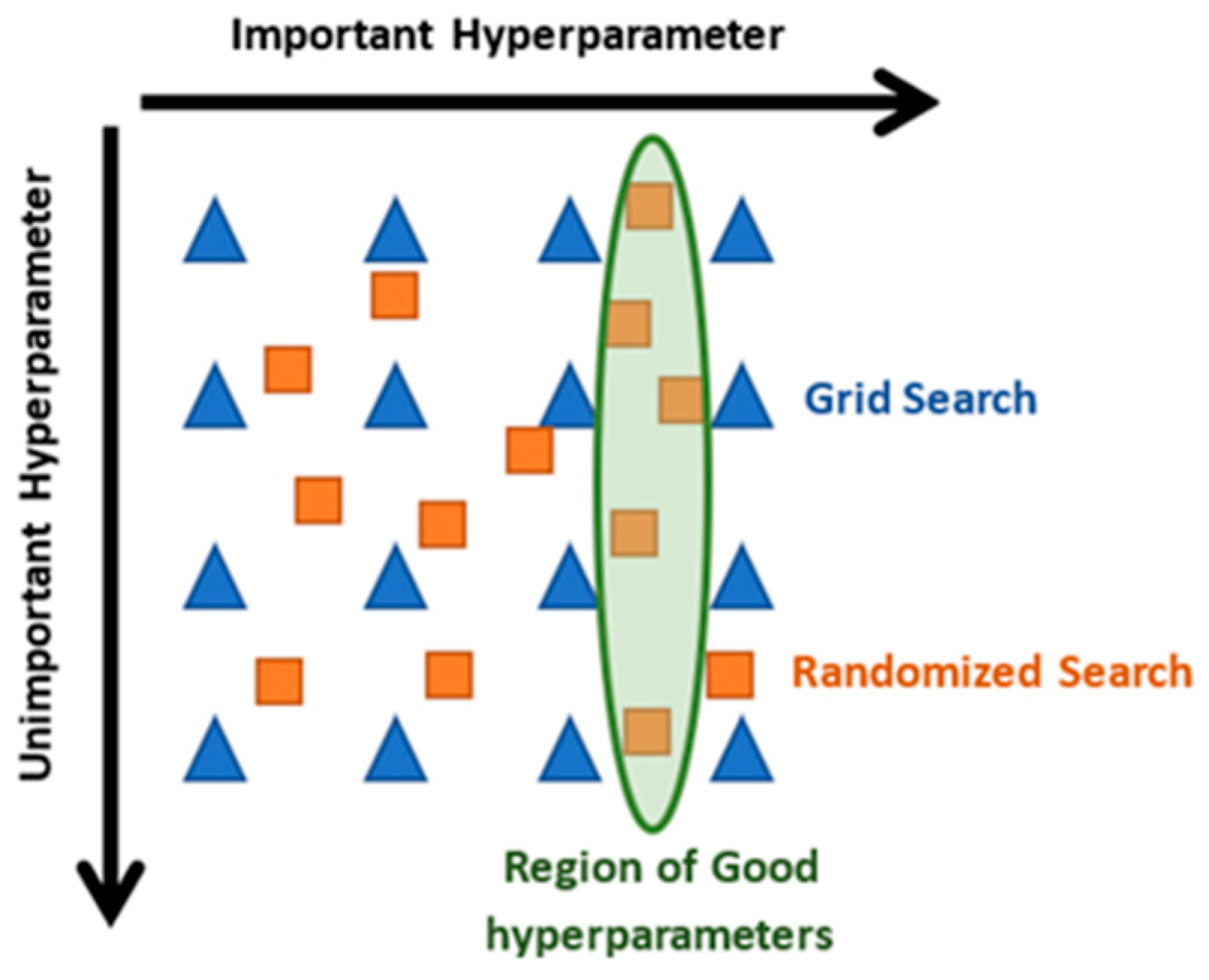
Unlike the grid search, not all attributes are used. This grid search searches exhaustively through every combination of well-defined hyperparameter values, significantly increasing the processing time. However, the random search is based on taking a constant magnitude sample of attribute configurations determined by the distribution of their values [
38]. The fact of using a random search allows finding a more diverse region of hyperparameters, contrary to what happens when establishing a grid with constant separation intervals, this has the advantage that the algorithm can find a region of hyperparameters that were not in the originally defined grid, as shown in
Figure 1.
Although it does not guarantee to find the hyperparameters that find the best combination of parameters, it is good enough to achieve a very good combination very quickly, this feature is essential, particularly when working with datasets in the field of astronomy, as there is usually a very large number of observations, a fact that generates a considerable processing time [
39]. By implementing this hyperparameter search and optimization technique, it is possible to achieve results that can compete with state-of-the-art algorithms, not only in performance but also in processing time.
3. Results and Discussion
The present section is relevant to the purposes of this article. Its relevance lies in the fact that the experimental results shown here will demonstrate the importance and relevance of using random forests in classifying stars, quasars, and galaxies. This information could support scientists since it will allow them to select a family of algorithms that is effective and efficient to carry out tasks of classification of astronomical objects. The relevance is evident when considering the possibilities currently offered by the state of the art of machine learning.
This section consists of six subsections.
Section 3.1 describes the validation method used to present the results of the experiments on the classification of astronomical objects.
Section 3.2 describes the performance measures used to present the results.
Section 3.3 contains descriptions of five classifier algorithms, the most important approaches to the state of the art, and references supporting the conceptual structures on which these algorithms rest.
The results of these state-of-the-art algorithms are presented in the remaining three
Section 3.4,
Section 3.5 and
Section 3.6. In
Section 3.4, the results of applying the random forest algorithm proposed in this work to the SDSS-DR14 dataset are presented, including tables and, importantly, the analysis and discussion of comparative results with different machine learning algorithms mentioned in
Section 3.2. Similarly, in
Section 3.5 and
Section 3.6, the data from the other two datasets, SDSS-DR16 and SDSS-DR17, respectively, are used to develop and evaluate the proposed algorithm. All of this will be of great support for measuring the performance of the proposed algorithm and its potential relevance in state-of-the-art machine learning and its applications.
3.1. Validation Method
In machine learning, every pattern classification experiment consists of two phases: the learning phase (also called the training phase) and the testing phase. To carry out both phases, validation methods are applied to the datasets to apply the classification algorithm.
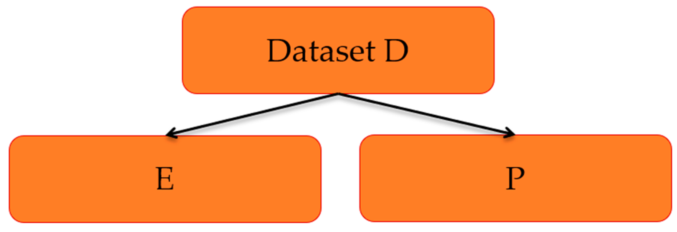
A validation method splits the dataset D into two disjoint or non-overlapping sets: a training set E and a test set P, so that sets E and P form a partition of dataset D, as shown in
Figure 2.
The patterns in the training set
E must be disjoint from the patterns in the testing set
P; therefore, the sets
E and
P must form a partition, that is:
Among the most popular validation methods in recent publications, three stand out: k-fold-cross-validation [
40], Leave-one-out [
41,
42], and Hold-out [
43]. To report the results in this work, we have selected the stratified Hold-out partition method with an 80–20 partition; that is, in each of the sets
E and
P, all classes are represented proportionally, with 80% of the patterns for algorithm training and 20% for testing.
3.2. Performance Measures
In machine learning, every pattern classification experiment consists of two phases: training and testing. After applying the selected validation method to the dataset (in our case, we have selected Hold-out 80-20), the pattern classification algorithm is executed on the training set E (in our case, the proposed random forest algorithm). Then, the trained algorithm is presented with one-by-one test patterns from the set P. The classification algorithm will output one of two options: correct or incorrect.
With these values, it is possible to calculate the measure that expresses the classification algorithm’s performance on the specified dataset with the selected validation method [
30]. In this paper, we will apply the proposed random forest algorithm to the SDSS-DE14, SDSS-DE16, and SDSS-DE17 datasets, with partitions generated by the Hold-out 80–20 validation method.
One of the simplest and easiest to calculate performance measures is accuracy [
44], defined as the ratio of correct predictions to the total number of test patterns. The value of accuracy ranges from 0 to 1.
The accuracy performance measure considers classification errors in general. However, in the calculation of accuracy, the costs of different types of errors are not considered; that is, it is equally important to misclassify a pattern from class 1 as misclassifying a pattern from class 2. In an imbalanced dataset, there is a real risk that a classifier (no matter how good it is) will exhibit a bias towards the majority class, ignoring the minority class. The solution to this problem is addressed using the confusion matrix, which allows for considering the particularities of the decisions made by state-of-the-art classifiers.
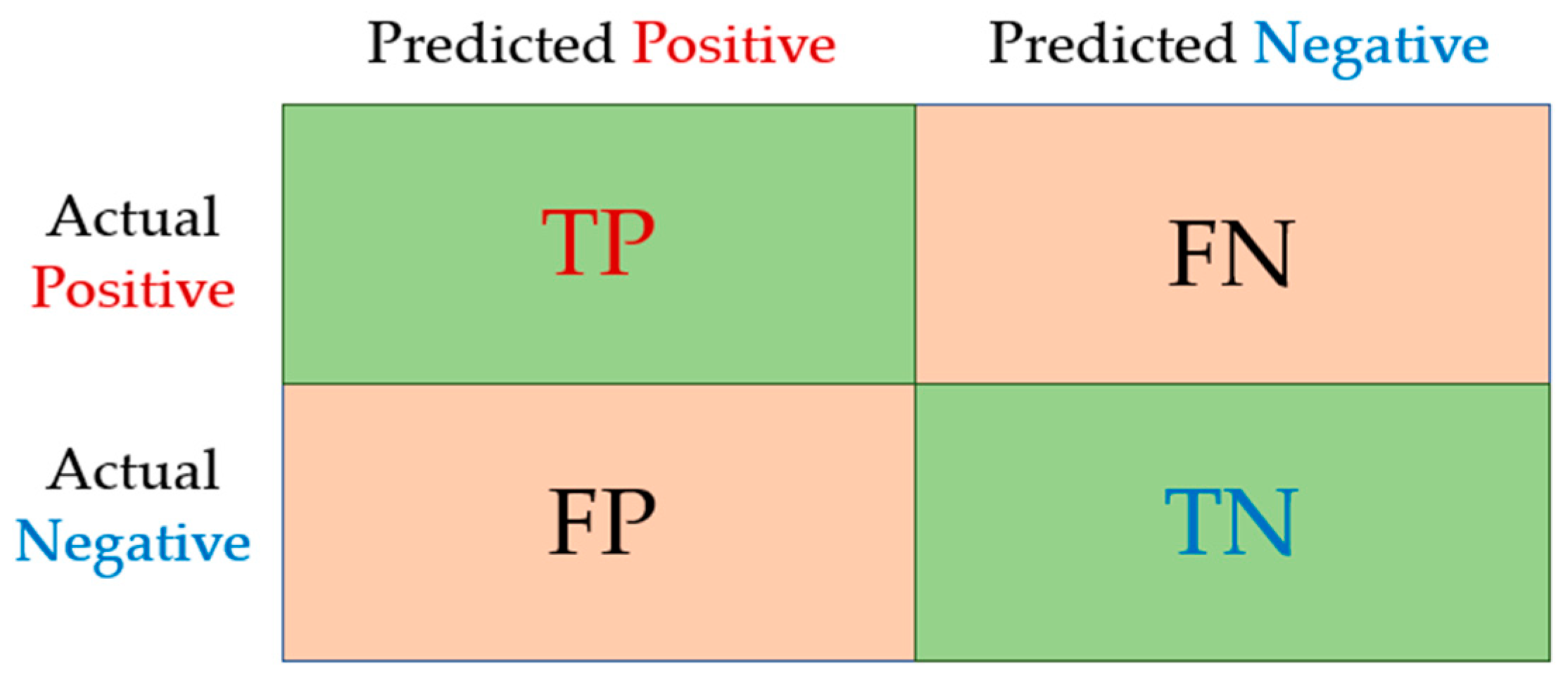
To work with the confusion matrix, it is necessary to define one of the classes as positive and the other class(es) as negative. From there, four possibilities arise that are shown below in a confusion matrix for two classes:
Where:
TP: True Positive
TN: True Negative
FP: False Positive
FN: False Negative
True Positive (TP) represents the number of positive patterns that are correctly classified as positive. In contrast, True Negative (TN) represents the number of negative patterns correctly classified as negative. False Positive (FP) is the number of negative patterns that are incorrectly classified as positive, and False Negative (FN) is the number of positive patterns that are incorrectly classified as negative.
The confusion matrix for three or more classes is simply an extension of the scheme in
Figure 3.
From the four elements of the confusion matrix, it is possible to define many performance measures. Next, we present the four performance measures used in the experiments of this paper, including the expression of accuracy in terms of the four elements:
TP,
FN,
FP, and
TN [
45,
46].
What happens to the values of accuracy and balanced accuracy when the value of IR increases?
Noticeably, as the value of IR increases, the performance measure balanced accuracy becomes more reliable than accuracy, due to the tendency of most classifiers towards highly imbalanced datasets: classifiers exhibit bias towards the majority class.
The balanced accuracy performance measure is more reliable than accuracy because it considers the contributions of both classes in the average [
46].
3.3. State-of-the-Art Classifiers for Comparison
This subsection concisely describes the conceptual basis of five of the most important state-of-the-art classifiers implemented on the WEKA platform [
47]. These are the classification algorithms against which the random forest algorithm proposed in this paper, will be compared. The proposed random forest algorithm was implemented in Python, using the scikit-learn library [
48].
The Naïve Bayes classifier is a probabilistic algorithm with a superstructure based on Bayes’ theorem. The classifier assumes that the features are independent of each other, which is why it has the naïve name.
IBk (Instance-based classifiers) is a family of classifiers based on metrics, which arises as an improvement to the k-NN family of classifiers (the k nearest neighbors). The difference between these two families of classifiers is that IBk can classify patterns with mixed features and missing values, thanks to the use of the HEOM metric. (Heterogeneous Euclidean–overlap Metric) [
49].
Support vector machines (SVMs) are a popular and powerful machine learning algorithm used for classification and regression analysis. SVMs aim to find the hyperplane that best separates the data points of different classes in a high-dimensional space. The hyperplane is chosen to maximize the margin, which is the distance between the hyperplane and the closest data points of each class. SVMs have shown high performance in various applications, including text classification, image classification, and bioinformatics. In this paper, a version of SVM called SMO is used, which is implemented in the WEKA platform. [
47]
The multi-layer perceptron classifier is an artificial neural network consisting of multiple layers, which allows for solving non-linear problems. Although neural networks have many advantages, they also have their limitations. If the model is trained correctly, it can give accurate results, in addition to the fact that the functions only look for local minima, which causes the training to stop even without having reached the percentage of allowed error.
A summary of the five algorithms against which the random forest algorithm will be compared is included in
Table 1.
3.4. Results and Comparative Analysis for the SDSS DR14 Dataset
As previously specified in
Section 2.1, the Sloan digital sky survey DR 14 dataset contains 4998 observations of the galaxy class (GALAXY), 850 of the quasar class (QSO), and 4152 of the star class (STAR). The imbalance ratio for this dataset is
IR = 5.88.
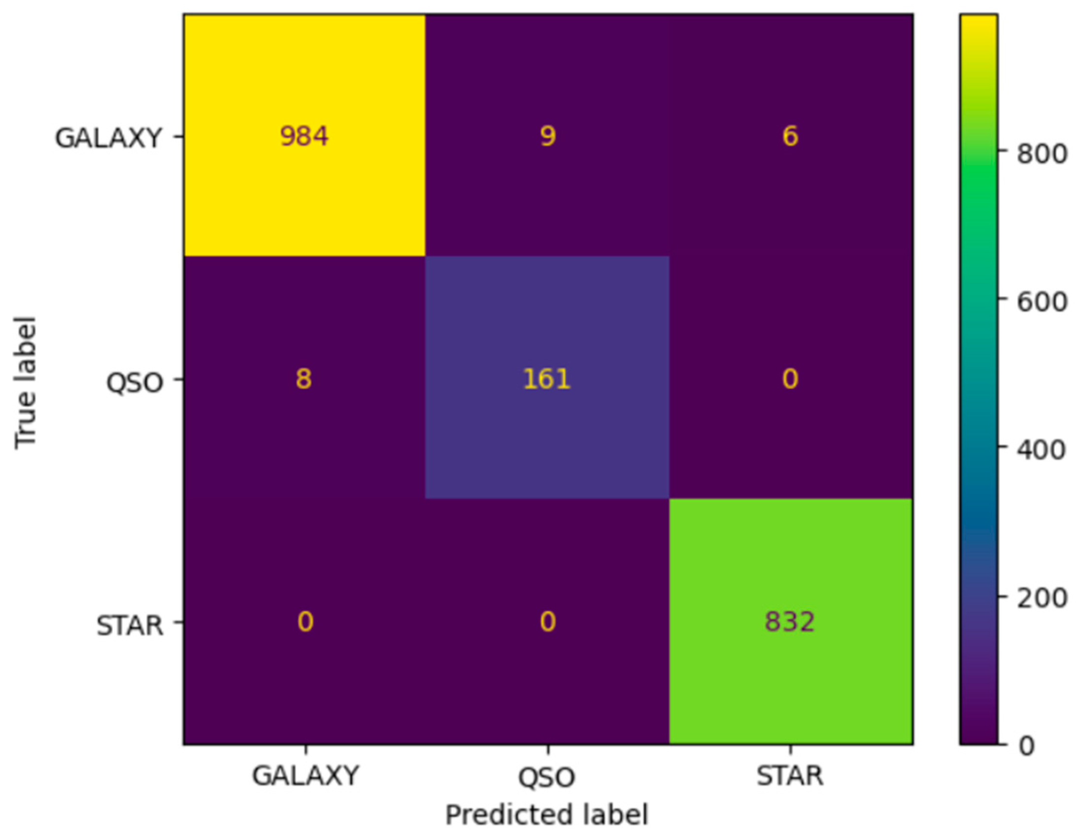
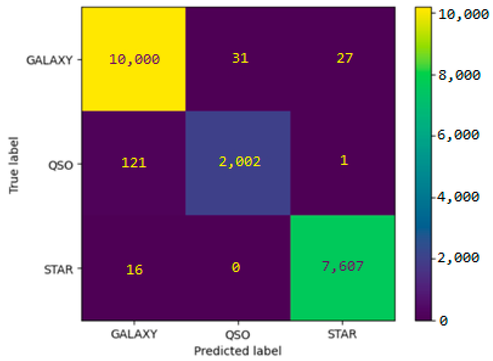
When running the proposed random forest algorithm on the SDSS DR14 dataset, the following confusion matrix is obtained (
Figure 4):
If we consider the case GALAXY as positive, the values of the three performance measures: sensitivity, specificity, and balanced accuracy, are calculated based on the values in the confusion matrix. For comparative purposes, the values of these four performance measures are included in
Table 2.
The results obtained by the proposed random forest algorithm on the SDSS DR14 dataset are good in all four performance measures.
The comparative table shows that the proposed random forest algorithm outperforms the other five state-of-the-art classifiers, considering GALAXY as the positive class.
The same applies when changing the positive class. Although these two additional results were not included, in both cases, the superiority of the proposed random forest algorithm persists.
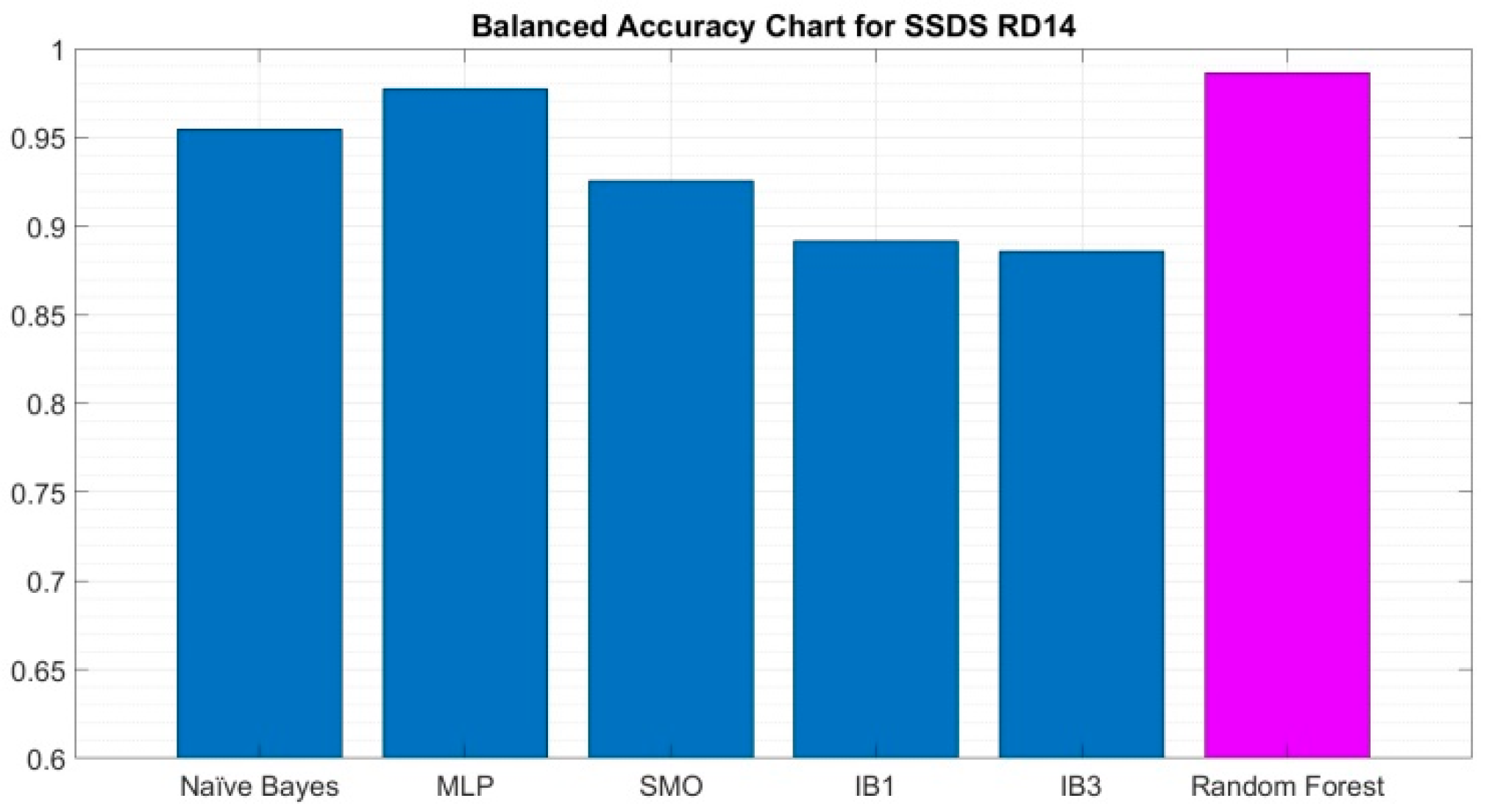
It is relevant to note a significant fact: despite the high-class imbalance in the SDSS DR14 dataset, which deviates from the IR 1.5 value specified for balanced datasets, the proposed random forest algorithm outperforms all others in the performance measure: balanced accuracy.
These results are shown graphically in the bar chart of
Figure 5 for balanced accuracy.
3.5. Results and Comparative Analysis for the SDSS DR16 Dataset
As previously specified in
Section 2.1, the Sloan digital sky survey DR 16 dataset contains 51,323 observations of the galaxy class (GALAXY), 10,581 of the quasar class (QSO), and 38,096 of the star class (STAR). The Imbalance ratio is
IR = 4.85.
Figure 6 shows the corresponding confusion matrix:
If we consider the case GALAXY as positive, the values of the four performance measures: accuracy, sensitivity, specificity, and balanced accuracy are calculated based on the values in the confusion matrix. For comparative purposes, the values of these four performance measures are included in
Table 3.
In this case, when applying the proposed random forest algorithm on the SDSS DR16 dataset, the results in three of the four performance measures surpass the other classifiers. The exception is the performance of the MLP algorithm in sensitivity, which outperforms the proposed random forest algorithm. This means that the MLP algorithm is better than the proposed random forest algorithm in detecting the other two classes that are not GALAXY, which are QSO and STAR.
Despite the above, it still holds that despite the high-class imbalance in the SDSS DR16 dataset, the proposed random forest algorithm outperforms all others in both performance measures: accuracy and balanced accuracy.
These results are shown graphically in the bar chart of
Figure 7 for balanced accuracy.
3.6. Results and Comparative Analysis for the SDSS DR17 Dataset
As previously specified in
Section 2.1, the Sloan digital sky survey DR 17 dataset contains 59,445 observations of the galaxy class (GALAXY), 18,961 of the quasar class (QSO), and 21,594 of the star class (STAR). The Imbalance ratio for this dataset is
IR = 3.13.
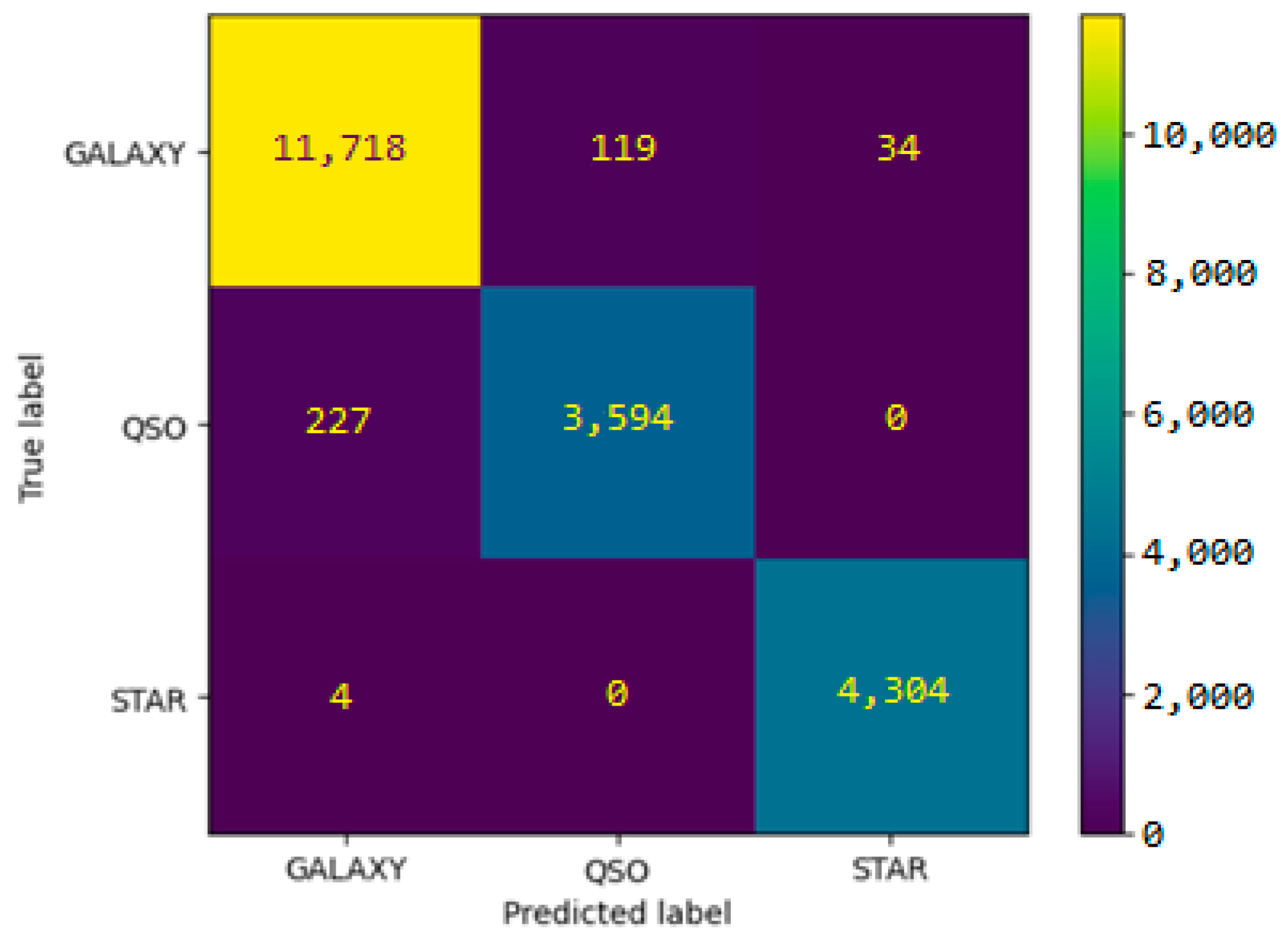
When running the proposed random forest algorithm on the SDSS DR17 dataset, the following confusion matrix is obtained (
Figure 8):
If we consider the case GALAXY as positive, the values of the four performance measures: accuracy, sensitivity, specificity, and balanced accuracy are calculated based on the values in the confusion matrix. For comparative purposes, the values of these four performance measures are included in
Table 4.
Again, the results on the SDSS DR17 dataset are similar to those obtained by the proposed random forest algorithm on the SDSS DR14 dataset, which are good in all four performance measures.
The comparative table shows that the proposed random forest algorithm clearly outperforms the other five state-of-the-art classifiers, considering GALAXY as the positive class.
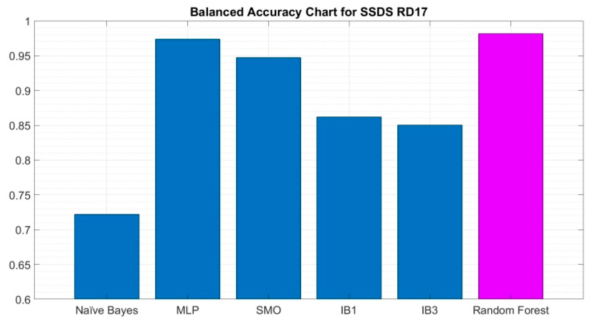
It is also worth noting that the proposed random forest algorithm outperforms all others in both performance measures: accuracy and balanced accuracy.
These results are shown graphically in the bar charts of
Figure 9 for balanced accuracy.
Given the results in
Table 2,
Table 3 and
Table 4, unusual behavior is observed within the pattern classification task [
50]. It is observed that for the set SDSS DR14, whose unbalance rate is the highest (
IR = 5.88), a better performance is achieved compared to the most recently created datasets, SDSS DR16 and SDSS DR17, this for the most reliable performance measure for unbalanced datasets, the balanced accuracy [
51]. In this circumstance, it cannot be established that the unbalanced factor determines the performance, but it can be attributed to the data acquisition; although the attributes considered for each dataset are the same, it should be remembered that these data are obtained from photometric signals, and being acquired in different seasons of the year, these can provide better or worse information of the phenomena occurred [
52].
Remarkably, the performance metrics shown for the SMO and MLP algorithms are extremely close concerning the performance achieved by the random forest algorithm proposal developed in this work. However, in that sense, it is evident that RF improves the results achieved by the algorithms of greater scientific relevance, although this difference in some measures seems to be minimal. In this circumstance, it is important to demonstrate that the results are reliable by applying statistical significance tests, these tests consist of accepting or rejecting the null hypothesis
, i.e., that there are no significant differences between one group of data and another. In this regard, the Friedman test will be used [
53] to identify whether there are significant differences between the performance results achieved by the proposed classification algorithms.
Looking at
Table 2,
Table 3 and
Table 4, the results for the different metrics calculated are similar between the algorithms. However, after performing Friedman’s statistical test, the null hypothesis was rejected with a confidence level of 95%, and a
p-value of 0.0262, which provides evidence showing statistically significant differences between the classifiers. In addition, the RF algorithm was ranked best according to Friedman’s mean rank for the methods compared, while the SMP and MLP algorithms ranked fourth and fifth, respectively, as shown in
Table 5.


 ,
, 


