Article

An Effective Local Particle Swarm Optimization-Based Algorithm for Solving the School Timetabling Problem

by
Ioannis X. Tassopoulos
1,
Christina A. Iliopoulou
2,
Iosif V. Katsaragakis
1 and
Grigorios N. Beligiannis
1,*
1
Department of Food Science and Technology, University of Patras, Agrinio Campus, G. Seferi 2, GR-30100 Agrinio, Greece
2
School of Rural and Surveying Engineering, National Technical University of Athens, 9 Iroon Polytechneiou Str., GR-15780 Athens, Greece
*
Author to whom correspondence should be addressed.
Algorithms 2023, 16(6), 291; https://doi.org/10.3390/a16060291
Submission received: 29 April 2023 / Revised: 12 May 2023 / Accepted: 1 June 2023 / Published: 4 June 2023
(This article belongs to the Collection Feature Paper in Metaheuristic Algorithms and Applications)

Abstract

:
This paper deals with the school timetabling problem. The problem was formulated as encountered in a typical Greek high school. A local version of the particle swarm optimization algorithm was developed and applied to the problem at hand. Results on well-established benchmark instances showed that the proposed algorithm achieved the proven optima provided from an integer programming method presented in earlier research. In almost all cases, the current algorithm beat the integer programming method, either concerning the lower bound yielded or the execution time needed.

1. Introduction

In the present paper, we deal with the high school timetabling problem (HSTP) as encountered in a typical Greek high school. The HSTP deals with the assignment of teachers to groups of students, called classes, in a predefined number of periods, called timeslots, in a predefined number of rooms. The corresponding assignment should be performed such that several constraints under consideration are not violated. More specifically, there are constraints that should be respected in any case, which are referred to as hard constraints. A timetable that fulfills all hard constraints is called a feasible timetable and can be applied at the corresponding school. Nevertheless, to apply a timetable in a high school, feasibility is usually not sufficient, as the timetable must be of high quality, as well. This means that several additional constraints must be satisfied; although, in practice, this is rarely accomplished completely. The greater the number of these constraints that are met, the higher the quality of the timetable becomes. These constraints, the satisfaction of which is preferable but not obligatory, are called soft constraints. A timetable that is feasible and respects the soft constraints to a high degree is referred to as an efficient timetable.
Solving the school timetabling problem to optimality is a hard task. In fact, the execution time needed to solve it rises at least exponentially in relation to the problem size. Informally speaking, problems with this property are called NP-Complete. It is likely that there is no exact algorithm that is able to solve these problems to optimality in a polynomial execution time. Pillay [1] categorized this problem into the class of NP-Complete problems depending on the constraints involved. In fact, the school timetabling problem becomes NP-Complete if constraints related to teachers’ availability are included [2,3]. Additionally, it is true that HSTP can be solved in polynomial time in some trivial cases, i.e., when no unavailability periods of teachers exist, or no co-teaching cases appear [2,3,4]. However, this is rare in real world situations. Usually, both teacher unavailability and co-teaching are present, at least in Greek high schools. The reader who is interested in the complexity of the school timetabling problem, as well as other educational timetabling problems, is referred to the contributions of Lewis [3], Bettinelli et al. [5], and Willemen [6].
Reasonably, the problem attracted the interest of many researchers over the years, with various solution approaches for devising efficient timetables presented [7]. There are several variants of the problem featuring different constraints, depending on each country’s educational system. This study focuses on the HSTP as encountered in Greek high schools and develops a local version of particle swarm optimization (PSO) to generate new lower bounds for the instances at hand. The performance of the algorithm is validated using benchmark data from Greek high schools and compared with existing algorithms.
The contribution of the present paper is two-fold. First, the local particle swarm optimization-based algorithm presented provides new lower bounds for the data set used. Second, to the best of our knowledge, this is the first time a local version of the PSO algorithm is applied to the school timetabling problem. Although there are several publications related to timetabling problems such as university course timetabling and exam timetabling problems, there is no publication solving the school timetabling problem using PSO, except for the works of Tassopoulos and Beligiannis [8,9,10]. The interested reader is kindly asked to refer to a recent survey [7] in order to verify this claim. The present algorithm is an extension of the works of Tassopoulos and Beligiannis [8,9,10], but it differs from them in several crucial points. Notably, the current algorithm is based on the local version of PSO, whereas previous works were based on the global version. The main difference between the global and the local version is that in the local version, there are several neighborhoods instead of one consisting of the whole swarm (see Section 4.3 for more details). In addition, it utilizes a backtracking schema that is activated in case the algorithm becomes stuck in a local optimum and is unable to update the global best result. In other words, the backtracking schema is activated when the global best remains the same for a number of cycles, called generations. Moreover, two refining procedures are used, instead of the one used in the previous works. In addition, several adjustments were made, resulting in new parameter values with a better outcome. Finally, we test our algorithm using the data set described in Section 5.1. The algorithm exhibits a high-quality performance and compares favorably to all other published soft computing algorithms applied to the same input instances. In addition to producing comparable results to the algorithms presented by Skoullis et al. [11] and by Tassopoulos and Beligiannis [8], which are the state-of-the art as far the input data set we use is concerned, it also compares favorably to the algorithm presented by Tassopoulos et al. [12]. The latter algorithm constitutes an integer programming method that yields optimal values and/or new lower bounds for the data set at hand, so far outperforming all methods applied to the Greek dataset [7]. The former method, despite introducing new lower bounds in some cases, fails to find the optimal solution for all instances in this data set. This fact was our primary motivation for designing and implementing a new algorithm. To be precise, our goal was not to implement an algorithm that would outperform all existing algorithms in terms of the best, average, and worst-case scenarios. Instead, our aim was to invent an algorithm that would uncover new lower bounds that were previously not discovered by the integer programming method. The current contribution does, in fact, reveal new lower bounds. Additionally, it achieves the proven optima introduced by [12] and manages to beat the integer programming approach either in terms of the execution time needed or the final score produced; for instance, that were not solved to optimality. The determination of new lower bounds confirms our hypothesis on the superior performance of the local version of PSO which can be comparable to integer programming in terms of the best solution produced. This is a rather important finding, considering that it is a single timetable that will be adopted by a school; thus, we are particularly interested in the best solution obtained.
This paper is organized as follows. Section 2 presents a brief overview of the relative literature on the HSTP. In Section 3, the formal definition of the Greek HSTP is given. The hard constraints along with the soft constraints and the evaluation function are presented. Section 4 consists of a brief presentation of the PSO algorithm for a continuous search space, a presentation of the primary distinction between the global version of PSO and the local version devised. Furthermore, it outlines the main technique that provides the particles with the ability of moving in a discrete search space in a similar way to their movement in a continuous search space. Additionally, the fundamental structural procedures of the proposed algorithm along with the pseudo code of the proposed algorithm are stated. Section 5 presents a comparative study of the results achieved by the presented algorithm with the results provided by other published algorithms using the same input dataset. The paper is concluded in Section 6 with a discussion of certain issues of the presented work. Additionally, thoughts about possible application of the algorithm to other timetabling problems along with future research plans of the authors are provided.

2. Some Previous Research on HSTP

In this section, we first mention some attempts to solve the school timetabling problem as it was defined in several countries with different educational systems. These attempts were based on exact methods as well as soft computing algorithms. Earlier work up to 1999 was reviewed in the study by Schaerf [13]. More up-to-date review work was provided by Pillay [1] and, more recently, Tan et al. [7].
The literature is rich with respect to approaches based on integer programming for the HSTP. Sørensen and Stidsen [14] used an integer programming method consisting of two phases for solving the problem as it appeared in Denmark. Post et al. [15] utilized a cyclic transfer algorithm to solve the HSTP in four Dutch high schools. Santos et al. [16] utilized an integer programming approach for HSTP, namely the class-teacher timetabling problem with compactness requirements (CCTPCR). They managed to present some strong lower bounds for Brazilian high schools. Sørensen and Stidsen [17] designed two mixed integer programming models for efficiently solving 100 real-life input data instances. Dorneles et al. [18] combined a mixed integer programming model with a fix-and-optimize heuristic along with a variable neighborhood search for the CCTPCR problem. Finally, we mention the work of Kristiansen et al. [19]. They addressed all the instances of the Third International Timetabling Competition (ITC2011), devoted to the HSTP, using a two-phase mixed integer programming model. In the first phase, they dealt with the hard constraints, while in the second phase, they dealt with soft constraints. They managed to produce new lower bounds in many cases.
Next, we discuss some initial attempts at using exact methods for solving the HSTP in Greece. Papoutsis et al. [20] utilized a column generation approach for the same problem, while a combination of constraint programming and operational research was used by Valouxis and Housos [21]. They managed to provide new lower bounds for some of the Greek input data sets. Moreover, Birbas et al. [22] dealt with the problem by dividing it into two stages. First, the assignment of the shifts was performed and afterwards, the entire timetable was constructed. In a recent approach, constraint programming was also employed by Demirović and Stuckey [23], exploiting various swap operators to improve solutions.
We continue the presentation of previous research on HSTP with some soft computing attempts. Saviniec and Constantino [24] proposed an algorithm based on iterated local search and variable neighborhood search using 34 real-world instances along with 7 other ones. Their algorithm outperformed all other algorithms on this data set and yielded the best solution for 38 out of 41 instances. The subsequent study by Saviniec et al. [25] proposed an algorithm based on parallelism that outperformed several stand-alone algorithms, such as iterated local search, tabu search, and simulated annealing, including two state-of-the-art algorithms by Dorneles et al. [19] and Fonseca et al. [26].
Soft computing attempts applied to the Greek HSTP are as follows. Zhang et al. [27] proposed a simulated annealing algorithm that outperformed all previous attempts on HSTP for the same instances. Tassopoulos and Beligiannis [8,9,10] presented three versions of global PSO. Skoullis et al. [11] presented a cat swarm optimization algorithm, which, together with the work of Tassopoulos and Beligiannis [8], constituted the state-of-the art on the Greek case HSTP. Meanwhile, Katsaragakis et al. [28] presented an algorithm based on artificial fish swarm optimization (AFSO), showing that AFSO cannot outperform PSO in this problem. Similarly, Tan et al. [29] hybridized PSO and hill climbing (HC).
Teixeira et al. [30] proposed two algorithms based on variable neighborhood search for solving ITC2011 instances. Saviniec et al. [31] proposed a cooperative parallel meta-heuristic solution algorithm that used a team of metaheuristics to construct and improve solutions for solving high school timetabling problems in Brazil. Odeniyi et al. [32] proposed an enhanced simulated annealing (ESA) algorithm to address high school timetabling problems in Nigeria. In the preprocessing step, a mixed integer linear programming technique was utilized to formulate the high school timetabling problem.
Last, a few studies examined the application of hyper-heuristics to HSTP. Ahmed et al. [33] presented a set of selection hyper-heuristics combining five different selection methods and three move acceptance methods. Pillay and Ozcan [34] presented generation construction hyper-heuristics for educational timetabling. The study investigated the automatic induction of two types of construction heuristics, namely, arithmetic heuristics and hierarchical heuristics.
We complete this literature review on HSTP by steering the attention of the interested reader to research conducted for the Third International Timetabling Competition (ITC2011). That competition was devoted to HSTP. We mention the research of the four finalists of the competition. The first team consisted of Fonseca, Santos, Toffolo, Brito, and Souza. They proposed (Fonseca et al. [35]) a simulated annealing algorithm incorporating iterated local search. They generated an initial solution using the KHE school timetabling engine of Kingston [36] and they refined it further. The second team, consisting of Domrös and Homberger [37], introduced a (1-1)-evolution strategy approach, yet did not achieve the best solutions known. The third team of Kheiri, Özcan, and Parkes proposed a hyper-heuristic which controlled some low-level neighborhood operators. Kheiri et al. [38] recommended their algorithm for solving similar academic problems such as university course timetabling and exam timetabling problem, since it was designed on an abstract level. Finally, the fourth team, consisting of Sørensen and Stidsen [17], proposed an adaptive large neighborhood search algorithm using tailored removal and insertion operators. The very good performance and flexible design of their algorithm rendered it suitable for other scheduling problems as well.

3. The Greek HSTP

The school timetabling problem deals with the assignment of teachers to classes during specific timeslots of the week, while fully respecting several constraints. Some other constraints can be violated, but it is desirable to satisfy them to the maximum extent possible. Those constraints that are mandatory are called hard, whereas the latter are mentioned as soft constraints. In a typical Greek high school, the rooms available for hosting the meetings between teachers and classes are sufficient, while for each teacher, the type and number of lessons, as well as the classes she/he teaches, are specified mainly by the director of the high school according to the existing legislation. In addition, the students are divided into classes appropriate for their age in alphabetical order. For the sake of brevity, we refer the interested reader to Skoullis et al. [11] for the full mathematical formulation of the problem.

3.1. The Hard Constraints

Typically, the following hard constraints, categorized in three sets, apply in a Greek high school. The first set contains the hard constraints which concern the classes, while the second set consists of the constraints that deal with the teachers. Last, the third set includes co-teaching constraints.
The hard constraints related to the classes are as follows:
  • Classroom conflicts: in each class, only one lesson must be taught at a given teaching time. Additionally, in each class, at most, one teacher teaches during any given teaching time slot, except for cases of co-teaching;
  • Idle periods of classes: idle periods for a class, i.e., hours when a class has no lesson, must be scheduled at the end of the daily teaching hours.
The hard constraints for the teachers are as follows:
3.
Teacher conflicts—parallel teaching: every teacher, in each time period, must teach one class at most;
4.
Teacher Availability: each teacher must be assigned to teaching hours during which she/he is available at each specific school. This constraint is typical in Greek high schools, since many teachers usually teach in more than one schools to reach their obligatory teaching hours;
5.
Teacher–class–course assignment: the number of hours and courses assigned to each teacher for instruction in each class is fixed and predetermined by the entry data.
Finally, the hard constraints concerning co-teaching are as follows:
6.
If two teachers must teach at the same time in the same class, then both must be assigned to this class during the co-teaching hours;
7.
If two teachers are required to teach in two different classes at the same time, their respective teaching periods should coincide with each other. This happens, for example, when two different classes are divided to form a class of “beginners” and a class of “intermediates” for the lesson of “Foreign Language”. These classes should be taught at the same time by different teachers.

3.2. The Soft Constraints

The soft constraints, which apply to the proposed version of the school timetabling problem, are as follows:
  • Course allocation—class dispersion: each teaching subject must be taught once in a class during a day at most;
  • Distribution of teachers’ hours—teacher dispersion: each teacher must have a balanced distribution of her/his working hours (teachings) in the days she/he is available;
  • Idle hours of teachers: each teacher must have a solid teaching schedule in each day, i.e., periods of inactivity between two consecutive teaching hours are not allowed. This is a typical constraint in Greek high schools, since teachers prefer to teach in successive hours with the minimum possible number of gaps.

3.3. The Evaluation (Fitness) Function

We used a weighted sum function that is based on hard and soft constraint violations to assist the algorithm’s evolution. Each constraint violation added a cost to the function value, which was estimated by the mathematical formula presented at the end of this section. The cost contribution of each constraint violation was computed via a formula that was different for each constraint. Next, we present the weights used in the fitness function along with the formulas for each constraint violation, whether it was a hard or a soft constraint. The actual values of these weights are presented in Section 4.7, in Table 2.
  • Hard Constraint Weight—HCW: This weight is used by the algorithm to distinguish between feasible and non-feasible timetables. This specific weight should be considerably higher than the value of the other weights, so that feasible but not efficient timetables should rarely have a higher total cost than the non-feasible ones. However, this weight should not be too large, to avoid restricting the diversity provided by infeasible timetables during the algorithm’s evolution;
  • Teachers’ empty periods weight—TEPW: this weight is related to the gaps in teachers’ schedules during a working day;
  • Ideal dispersion weight for teachers—IDWT: this weight is used to compute the dispersion of teachers’ hours of teaching;
  • Ideal dispersion weight for classes—IDWC: this weight regulates the ideal dispersion of teachings to classes.
A very important parameter is also the exponential basis used in the definition of objective function. It is symbolized with BASE and its value must be a real number between 1 and 2, as suggested by Tassopoulos and Beligiannis [8]. This parameter is used in various constraints. In the presented contribution, we decided to follow a different approach to the BASE setting value, from that proposed by the above-mentioned researchers, to avoid the production of infeasible final timetables. The analytical formulas for the cost of violating each constraint are listed next.
  • Hard constraints (see Section 3.1)
    • Classroom conflicts: this type of hard constraint is always respected by the representation of the particle as a matrix (see Section 4.4.1);
    • Idle periods of classes: for each class that has a gap that is not the last hour of the day, the following cost was added: H C W 2 B A S E B A S E , contrary to the proposal of Tassopoulos and Beligiannis [8], who use the formula H C W B A S E B A S E ;
    • Teacher conflicts—parallel teaching: for each teacher and for each period during which the teacher is assigned to more than one classes, i.e., K classes, the following cost was added: H C W B A S E k ;
    • Teacher availability: for every period a teacher is assigned to teach when she/he is not available on the corresponding day, the following cost was added: H C W B A S E 3 ;
    • Teacher–class–course assignment: this constraint is never violated due to the initialization process which is performed in accordance with the input data;
    • Co-teachings: the following cost was added for each class involved in co-teaching when the corresponding teacher was assigned to a period, while hers/his co-teacher is not assigned to the same period: H C W 2 B A S E B A S E , contrary to the proposal of Tassopoulos and Beligiannis [8], who use the formula H C W B A S E B A S E .
  • Soft constraints (see Section 3.2)
    • Course allocation—class dispersion: for each class, the following cost was added: I D W C H O U R S B A S E D A Y S , where H O U R S is the number of hours a subject is taught and D A Y S is the number of days when this takes place. For example, if a teacher is assigned to a class for three periods during a day, while she/he teaches only one lesson—subject in this class, then this subject occupies two hourly slots. Therefore, H O U R S = 2 .
    • Distribution of teachers’ hours—teacher dispersion: in this case, an important distinction from the proposal of Tassopoulos and Beligiannis [8] is proposed, since the concept of variable a b s o l u t e e r r o r is introduced. For each teacher, the following cost was added:
      I D W T a b s o l u t e e r r o r B A S E D A Y S , where a b s o l u t e e r r o r is the sum of the absolute values of the differences between the actual hours taught by the teacher in a day and the number of hours she/he should teach according to the ideal distribution. Additionally, D A Y S is the number of days in which the actual distribution is different from the ideal. For example, if the ideal allocation of hours for a teacher is the distribution “2, 2, 2, 2, 3” (with any permutation of these numbers considered as a valid ideal distribution), while the actual distribution of the teacher’s teaching hours is: “1, 0, 4, 4, 2”, then the value of a b s o l u t e e r r o r equals: | 1 − 3 | + | 0 − 2 | + | 4 − 2 | + | 4 − 2 | = 8 and days = 4.
    • Idle hours of teachers: for each teacher, the following cost was added: T E P W H O U R S B A S E D A Y S , where H O U R S is the total number of gaps within the teacher’s schedule and D A Y S is the total number of days where the gaps occur.
Next, following the detailed presentation of the method calculating the cost of each constraint violation and the corresponding formulas, the mathematical formula of the objective function (fitness function) is presented, which evaluates the quality of each particle.
f = c a s e s H C W B A S E 3 + c a s e s H C W B A S E k + c a s e s H C W 2 B A S E B A S E + c a s e s H C W 2 B A S E B A S E + c a s e s T E P W H O U R S B A S E D A Y S + c a s e s d i s p e r s i o n I D W T a b s o l u t e e r r o r B A S E D A Y S + c a s e s d i s p e r s i o n I D W C H O U R S B A S E D A Y S
The above function is minimized during the evolution of the proposed algorithm.

4. The Proposed Algorithm

4.1. The Particle Swarm Optimization Algorithm

The particle swarm optimization algorithm (PSO) was proposed back in 1995 [39]. It is a very popular optimization algorithm among researchers because of its simplicity, easy coding, and lack of many parameters to adjust. The initial version of PSO referred to continuous search spaces. Two years later, the same researchers proposed a version of the PSO for discrete search spaces [40]. In the following years, many variations of the PSO were published, exhibiting superior performance compared with the original versions. As far as the continuous search space is concerned, there were a many PSO variations, such as Simple PSO 2007 (SPSO 2007), Simple PSO 2011 (SPSO 2011), Balanced PSO, Tribes PSO, etc. The interested reader is referred to the respective web site [41], where there is a plethora of PSO variations, interesting code, and applications. For the problem at hand, the lack of a PSO version that could be universally applied is evident. It should be obvious that the continuous search space variations of PSO cannot be adopted in the case of a discrete space problem such as the school timetabling problem. The reason for this is the unique nature of discrete search space optimization problems, which makes it difficult to develop a uniform approach to modeling them.

4.2. The Original PSO for Continuous Search Space

The inventors of PSO presented it as an optimization method that can be applied in cases where the global minimum or global maximum is sought for functions with a continuous domain. The PSO simulates the behavior of a bird swarm, as its members are seek to fulfill a common purpose, i.e., searching for their food. According to the PSO jargon, the members of the swarm are called “particles”, while their movement over the search space is described as a “flight”. The food that the birds search for is simulated by the searched optima. It should be noted that the particles interact with each another, while there is a swarm memory that records the personal best position that any particle ever had during the search. Obviously, the best among these positions constitutes the global best position, in other words, the optimum or near optimum, which is recorded as well. The personal behavior of each particle, i.e., the chosen direction to fly, is influenced by its personal best position (personal component) and by the global best position (social component). If the position of each particle is denoted by a vector, the previous task is accomplished by the so-called “velocity vector”. At any generation, the velocity vector of each particle is added to the position vector of the particle itself. Thus, the change of the co-ordinates of each particle causes its movement from one point to another over the search space in a systematic way.

4.3. The Local Version of PSO

Each particle flies over the search space influenced by its personal experience, i.e., personal best ( P B E S T i ) and the social experience, i.e., global best ( G B E S T ) . The G B E S T is the structure of the best solution found among all particles up to the current generation. Hence, it could be said that the whole swarm forms a neighborhood consisting of all particles, and that each particle is informed by the members of this neighborhood, i.e., its neighbors. The above idea is the basis of the initially proposed PSO. Later, it was pointed out that this version had some drawbacks, as the algorithm often became stuck in local optima very early in the search. The so-called “premature convergence” is likely to be avoided by the local version of PSO, which is more sophisticated. The main difference between the global and the local version is that in the local version, there are several neighborhoods, instead of one consisting of the whole swarm. In other words, the particles are grouped to form different neighborhoods. Each neighborhood has its own G B E S T which is used for informing particles.

4.4. A Proposed Local Version of PSO for Discrete Search Space

There are a lot of PSO variations for continuous search space. Theoretically, any of them can be used to solve any optimization problem with a continuous domain. Of course, the quality of the solution depends on the choice of the PSO variation. However, the situation is different when the optimization problem involves a discrete search space. Even though the relative literature is rich with published attempts dealing with optimization problems with discrete domains using PSO implementations, none of them can be universally applied to handle discrete search space optimization problems. The reason for this it the lack of a universal model representation for such problems. Combinatorial problems, such as timetabling, can be represented by various models that differ significantly from one another. Moreover, the application of the original PSO version is inappropriate in the case of a discrete domain. For instance, considering the velocity vector and adding it to the position vector of a particle would clearly cause the search to move beyond the problem’s feasible region. We have to mention that we indeed tried to apply the binary version of PSO [40] but the outcome was of a rather poor quality.
Therefore, it is clear that creating and deploying new algorithms for each discrete problem is necessary when it comes to the PSO case. However, any algorithm claiming to be PSO-based must maintain the essence of the original PSO. In our contribution, we present a PSO-based algorithm for solving the Greek school timetabling problem. We retained some basic design structures, while several fundamental changes were implemented as well. The most significant change was that we used the local version of PSO, unlike the global one used in other works. That is, instead of considering the swarm of particles as a whole neighborhood in which particles exchange position information with each other, we split the swarm to several neighborhoods. Each neighborhood is dedicated to a particle and consists of a standard number of particles—neighbors. The neighborhoods are not necessarily disjointed, and their topology is similar to those proposed at the respective website [41]. To be more precise, we used the random topology, i.e., we periodically update the neighborhood of each particle, at each generation, by selecting other particles as neighbors at random. Of course, each particle has a neighborhood, and within each neighborhood, there is a particle that is considered the best, known as the “local best” of that particle’s neighborhood. In previous works [8,9,10], each particle exchanged positional information with all the other particles through the “global best”, i.e., the particle with best quality in the total swarm. In addition, its trajectory is influenced by both the global best and its personal best, i.e., the best structure it ever had during the evolution, up to the current point. In the current work, the local best plays the role of the global best, while the personal best and global best keep informing each particle and influencing its trajectory as well. Since the trajectory of each particle is influenced by the local best, the personal best, and the global best, the claim that our algorithm constitutes a local version of PSO for a discrete domain problem such as the school timetabling one is rather justified. The exact way in which the local best, personal best, and global best particles influence the trajectory of each particle, allowing it to “fly” over the discrete search space is briefly described here in Section 4.4.2. The outcome of our algorithm indicates that the use of the local version of PSO outperforms the global PSO. Additionally, this fact was rather expected, and it is in accordance to what is already known for the PSO versions applied in continuous domain problems [42,43].
Another fundamental point in which our current work differs from previous ones is the use of a backtracking schema. To be precise, any time the algorithm reaches a certain number of cycles, called generations, without improvement due to stagnation, the particle is restored to the position it had at the beginning of the stagnation period.
Finally, the same idea of using a backtracking schema is present in a second refining phase that is added. In the present work, the algorithm used two refining phases instead of one proposed in previous works. Both refining phases were applied on global best after it was handed out by the main algorithm. More details on these procedures will be outlined in the following.

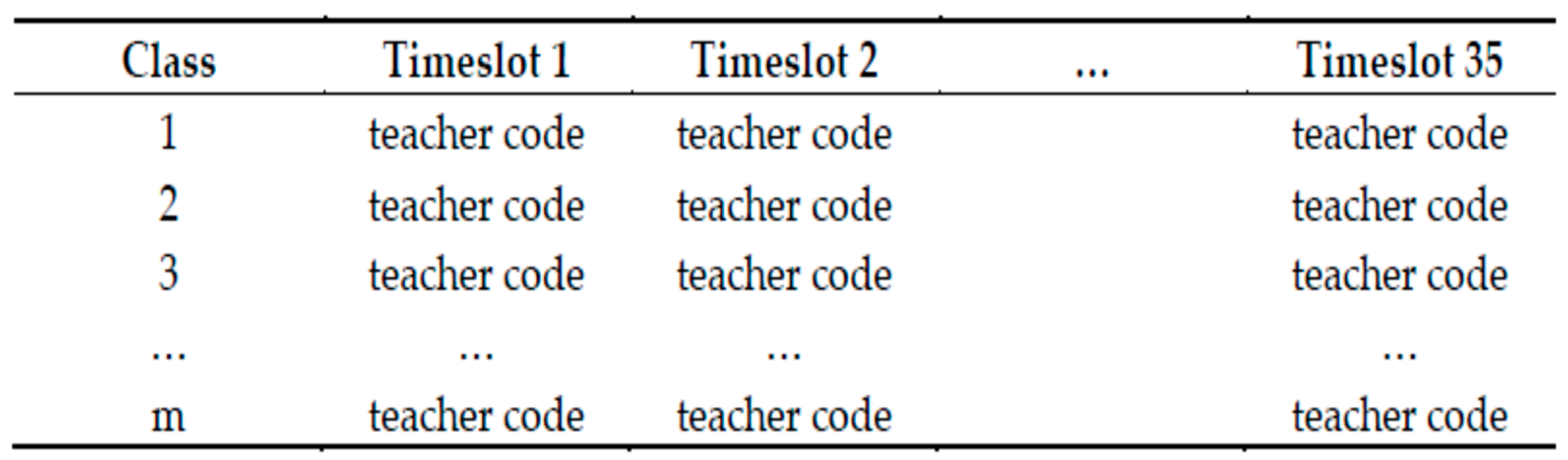
4.4.1. Particle’s Encoding for the HSTP

Each particle is represented as a matrix with as many rows as the number of classes determined by the input file and 35 columns. Each column represents a timeslot. In a typical Greek high school, the lessons take place in five days, from Monday to Friday, over seven hours a day at most. Thus, any group of seven consecutive timeslots corresponds to a working day of the week. At each cell of the particle (matrix), we place the value of “−1” when the corresponding timeslot of the class is vacant. Otherwise, we place an integer number, different from “−1”, representing the code of a teacher. In Figure 1, we present the particle’s structure.

4.4.2. Providing the Particles with Flying Ability

In this contribution, we take advantage of an idea already presented in previous works, to provide the particles with the flying ability [9], i.e., to change their position within the search space, That is, we choose a random timeslot from a particle, called “source”. The particle used as the “source” is either the local best or the personal best or the global best. Unlike previous works, where the source particle can only be either the personal best or the global best, in this contribution, we also use the source particle as the local best. The mechanism is quite simple: when a timeslot is randomly chosen from the source particle, we replace the timeslot cells’ content of the particle with the corresponding cells’ content of the timeslot in the source particle. The substituted content of the particle cell is transferred to the best cell position among those of the corresponding row/class that have the same content with the source cell. The best cell position is the one yielding the best particle quality. In this way, we preserve the balance of the number of teaching hours for each teacher at any row/class she/he is assigned to teach. Evidently, this mechanism provides the particle with flying ability, i.e., it allows the particle to explore the search space by changing its structure. As explained above, the trajectory of each particle is not influenced just by its personal best and/or the global best. It is influenced by its local best, too, giving the algorithm a characteristic of a local version of PSO. The corresponding procedure is shown in Figure 2.

4.5. Fundamental Functions

As we previously mentioned, the present algorithm is an extension of previous works. Essentially, we use the same fundamental functions in the main algorithm. These are the “Swap_with_probability”, the “Insert_column” and a “While-loop-structure”. We refer the interested reader to previous works, where a detailed description of these functions is presented [8,9,10]. For the sake of completeness, these functions are shortly outlined in the next subsections. In addition, we use a backtracking schema which is activated any time the algorithm became stuck in a local optimum for several generations in the main algorithm and also in the second refining schema added.

4.5.1. Swap_with_Probability Function

This function takes a particle and two timeslots chosen at random as its input arguments. Its output is the particle itself. This function attempts swapping the content of all cells belonging to the same row/class and to the two corresponding timeslots. It accepts any swap that, if performed, yields a smaller or equal fitness value. In case the swap causes a conflict, it is accepted with a certain probability, which is empirically set to 50%. It may seem quite a big value, but after performing exhaustive experiments with several other values, we verified that 50% was the best choice, enhancing the diversification ability of the algorithm. Using other values, the algorithm was more prone to getting trapped in local optima.

4.5.2. Insert_Column Function

The input arguments of this function are a randomly chosen timeslot, a particle called “source” and a particle called “destination”, which is the output. In a nutshell, the randomly chosen timeslot from the “source” particle is inserted into the “destination” particle. In the main algorithm, the personal best, the global best, and the local best are used iteratively as the “source” particle for the local search. More comments on this function are present in Section 4.4.2 above, while a detailed description of it is given by Tassopoulos and Beligiannis [8].

4.5.3. While-Loop-Structure

The last thing that is in common with our previous works is a while-loop-structure. The particle enters this structure where successive calls of “insert_column” are carried out. At each call, the input arguments of “insert_column” are the particle itself as the “destination”, the global best as the “source”, and a randomly chosen timeslot. The loop terminates if the fitness of the particle becomes equal to or smaller than the global best fitness. Moreover, any time the loop completes 10 cycles, there is a possibility to terminate the loop regardless of the fitness value of the particle. This kind of loop termination is performed with a probability value of 1.086%, which is empirically set.

4.5.4. Back-Tracking Schema

We use a back-tracking schema that is activated any time the particles do not evolve, that is, they are unable to improve their fitness. In such a situation, the phenomenon of stagnation is observed, and the particle is restored to the form it had before stagnation occurred. To identify stagnation, the number of generations without fitness improvement is empirically set to 150.

4.6. The Two Refining Schemas

We use two refining schemas to improve solution quality. Both schemas work on the global best particle produced by the main algorithm, and attempt to eliminate the idle time periods of the teachers. They influence the structure of the global best by swapping randomly chosen pairs of timeslot cells belonging to the same day. The days of the week are successively processed. At each day, a certain number of swaps is performed. In the first refining schema, this number is empirically set to 750,000, while in the second one, to 800,000.
The first refining phase is described as follows. First, the fitness for each day of the week is calculated for the global best, counting only hard constraint costs and the teacher gaps’ soft constraint costs. If this fitness value equals zero, i.e., the specific day violates no constraints, the local search procedure proceeds to the next day of the week. If a day with a positive fitness value is found, then two different timeslots are chosen and all possible swaps between these are performed, considering the corresponding acceptance probabilities. However, in this case, invalid swaps that increase the fitness are not accepted. Subsequently, the fitness of the newly formed day of the global best is calculated. If the new fitness value is equal to or lower than the original value, this day’s structure is copied to the structure of the global best, until a transformed day with an equal or better fitness is found.
The only other point that differentiates the first refining schema from the second, apart from the maximum number of swaps performed, is that in the latter one, there is a back-tracking mechanism, such as the one used in the main algorithm. Indeed, the second refining procedure acts as follows: if the algorithm is unable to update the global best, the search restarts from the last successful updating point. As it is easily derived, any modification caused due to these swaps cannot alter the violation cost of class-dispersion and/or the cost of teacher-dispersion, since these swaps take place within a day, while the two aforementioned constraints are computed based on the entire week’s timetable. Hence, such swaps could only improve the global best fitness by reducing the number of teacher idle periods. Please note that each refining schema is triggered only if there are teacher idle periods in at least one day of the week.

4.7. The Pseudo Code of the Complete Proposed Algorithm

In this subsection, we present the pseudo code of our algorithm.
1
Initialize Swarm_Size particles
2
Initialize personal best fitness of each particle and global best fitness to worst possible
3
for Max_Iter generations
4
    for each particle do
5
         Determine the neighborhood and l_best of current particle
6
         If fitness of current particle < p_best fitness then
7
            Update the p_best and the p_best fitness
8
             If fitness of current particle < g_best fitness then
9
                   Update the g_best and the g_best fitness
10
             End if
11
         End if
12
        Pick two different timeslots t1, t2, at random
13
        current particle ⟵ Swap_with_probability (t1, t2, current particle)
14
        Pick a timeslot t3 at random
15
        current particle ⟵ Insert_Column(current particle, t3, l_best)
16
        Pick one timeslot t4 at random
17
        current particle ⟵ Insert_Column(current particle, t4, p_best)
18
        Pick one timeslot t5 at random
19
        current particle ⟵ Insert_Column(current particle, t5, g_best)
20
        while fitness of current particle > g_best fitness
21
             Pick a timeslot t6, at random
22
             current particle ⟵ Insert_Column(current particle, t6, g_best)
23
             exit the loop with probability exit_loop_prob every exit_loop_times
24
         end while
25
         if stagnation happens for backtracking_tolerance generations
26
                Restore current particle
27
         end if
28
   end for each particle
29
end for Max_Iter generations
30
Terminate main algorithm and return g_best and g_best fitness
31
if teacher gaps exist then
32
      execute first refining schema
33
end if
34
if teacher gaps exist then
35
      execute second refining schema
36
end if
37
return global_best and fitness

4.8. Algorithm Parameter Settings

Table 1 presents all parameter values set for our algorithm, while in Table 2, we present the parameter values used for the fitness function of the Greek HSTP. All parameter values were set empirically (by trial-and-error). We conducted exhaustive experiments and selected the value that assisted the algorithm to achieve the best possible results for each parameter. This is common practice for population-based computational intelligence algorithms.

5. Testing the Proposed Algorithm

We tested our algorithm using a well-known data set consisting of real-world instances taken from the city of Patras, Greece. This benchmark data set is presented and analyzed in Section 5.1. Afterwards, in Section 5.2, we compare the proposed algorithm against two soft-computing algorithms, which, until now, were the state-of-the-art as far as the above-mentioned benchmark data set is concerned. The first of these attempts, presented by Skoullis et al. [11], was based on cat swarm optimization (CSO) algorithm. The second one was based on a global version of particle swarm optimization (PSO) algorithm and is presented by Tassopoulos and Beligiannis [8]. The two algorithms exhibited a similar performance. The second one was chosen to test the hypothesis that the local version of PSO we presented outperformed the global one. Eventually, it was verified that the local version of PSO outperformed the global one, at least in the case of the given data and the given problem. Apart from these two soft computing algorithms, we also included an integer programming method [12] in the comparison. The reason for choosing this method is that it was shown to produce the best results so far for this particular benchmark and even generated optimal results in some cases [7].

5.1. The Benchmark Data Set

To test the performance of the proposed algorithm, we decided to use the same data set used by other researchers that dealt with the Greek HSTP, which we also used in our previous publications. Using the same data set gives an insight about the relative strength of the algorithm in quite a fair manner. The data set we used consisted of ten input files, with six of them constituting the so-called “Beligiannis’ data set” [1,44,45]. It is true that the input data files of the above-mentioned data set may be considered of small to medium size. Nevertheless, we insisted on them firstly for historical reasons and for a fair comparison to other published algorithms, as we explained in the beginning of this section. Secondly, despite their size, these instances were not easy to solve. The interested reader is referred to Tassopoulos et al. [12], where a typical integer programming method was found unsuccessful in solving all of them. At this point, we would like to state that three of the ten input files, albeit not being the most difficult ones to solve, were used at the Third International Competition, in 2011. This competition was dedicated to the school timetabling problem. Three of these files, among others, were utilized as a benchmark for testing the competition finalists’ algorithms. Next, in Table 3, we present some main characteristics of these input files. They are numbered from 1 to 11, with the file numbered by 6 being absent. This is because the corresponding file had some documentation deficiencies. This fact caused the exclusion of file 6 from several published works. We followed the same exclusion practice. Files 8, 9, and 10 were presented by Valouxis and Housos [21], while files 8, 9, 10, and 11 were used by Papoutsis et al. [20]. Finally, the above set of files were used, except from Valouxis and Housos [21] and Papoutsis et al. [20], by Zhang et al. [27], Tassopoulos and Beligiannis [8,9,10], Raghavjee and Pillay [46], Katsaragakis et al. [28], Skoullis et al. [11], and Tassopoulos et.al. [12] in corresponding research works.
One may easily conclude that the used benchmark data set is quite interesting, since seven files out of ten include teacher unavailability cases, while four out of the six files of the Beligiannis’ data set include unavailability cases along with co-teaching cases. As was obvious in Section 5.2, where the performance of the proposed algorithm is presented and compared to other algorithms, files 7, 1, 2, and 4, in this order, were the most difficult ones. On the other hand, files 5 and 8 were quite easy to solve.

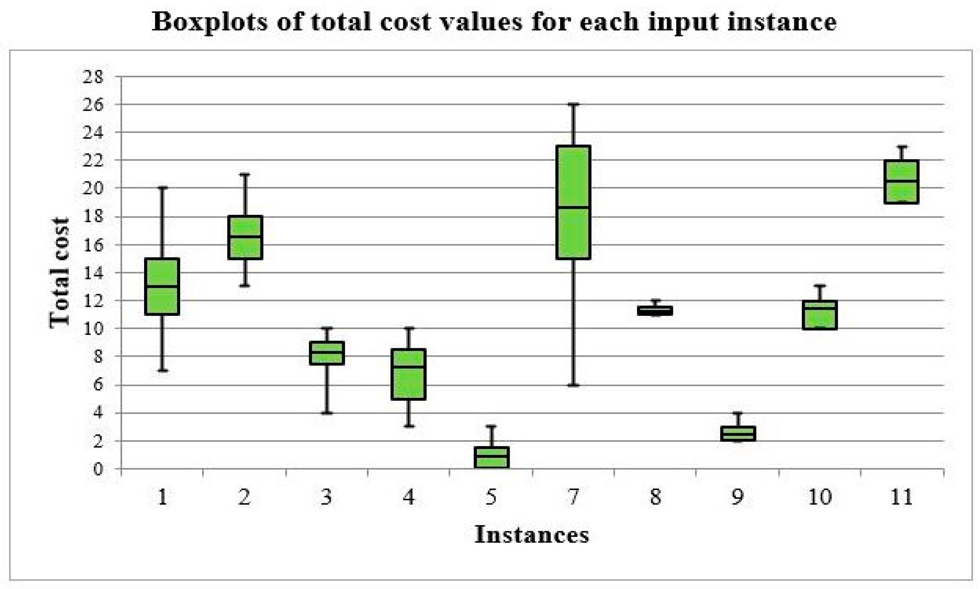
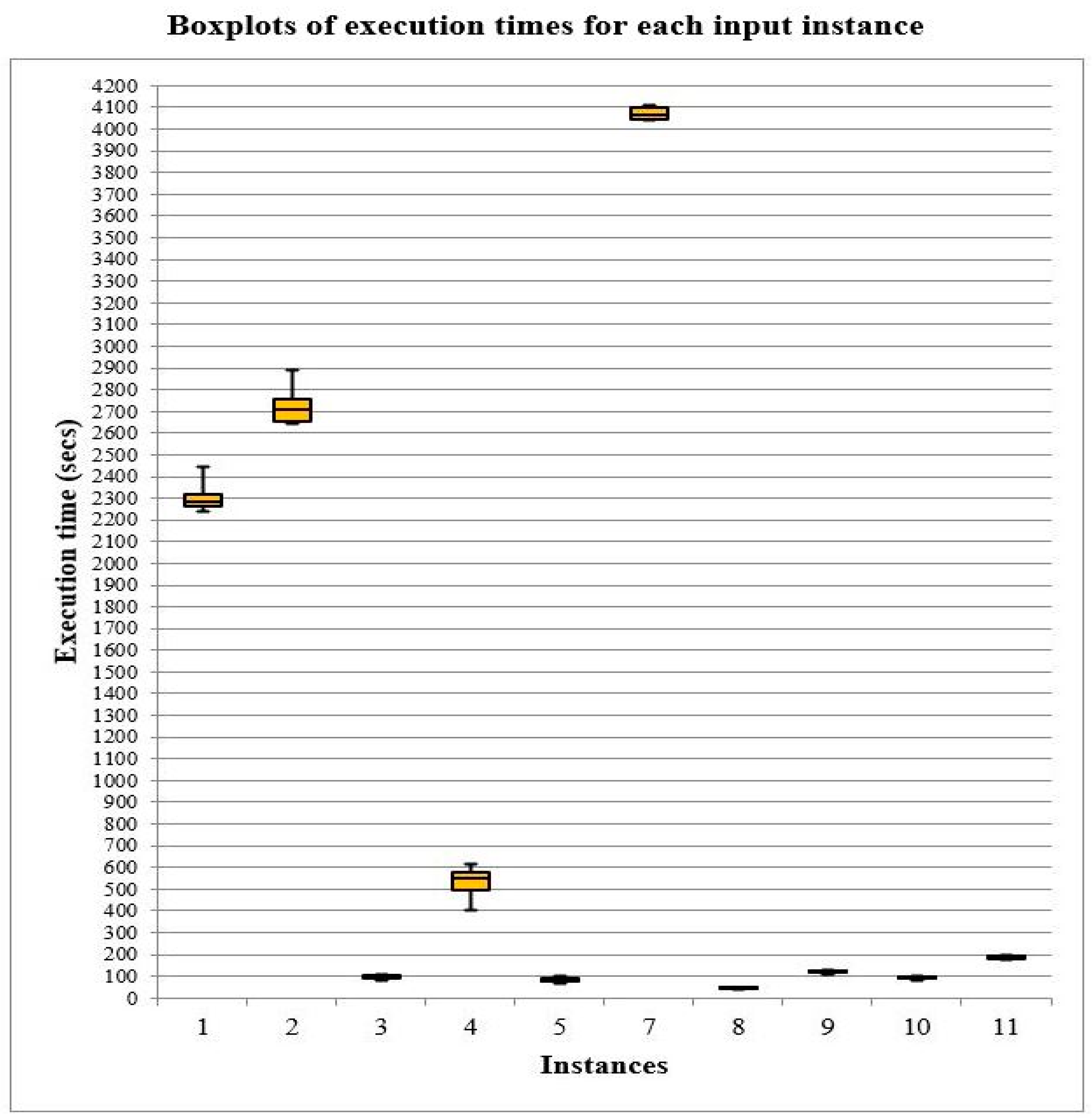
5.2. Performance of the Proposed Algorithm and Comparison to the State-of-the Art Algorithms

As stated before, we compared our algorithm with a global version of PSO proposed by Tassopoulos and Beligiannis [8] and a CSO algorithm by Skoullis et al. [11] along with an integer programming method presented by Tassopoulos et al. [12]. The choice of these three attempts was justified in Section 5 above. It should be noted that the same fitness function was used among the above-mentioned studies, under the same parameters shown in Table 2. We ran each algorithm 30 times for each instance. In our experiments, we used a PC with i-4770 intel CPU at 3.40 GHz with 16 GB of RAM. The OS was Windows 64 bit. The programming language we used was the same used for the other soft computing algorithms, with which we compared our present work, i.e., ANSI C. We first present, in Table 4, the comparison between the global version of the PSO and the current local version of the PSO algorithm. For each instance, the best, worst, and average score is presented along with the standard deviation (STD) and the coefficient of variation (CV). The corresponding values for the execution times are given, too. The best score between the two algorithms is indicated by bold. It should be highlighted that the score presented in the tables below corresponds to the number of soft constraint violations, i.e., one cost unit is added for each teacher idle hour, for each case of undesirable class dispersion (repetition) and each case of undesirable teacher dispersion. Hence, the reader should not confuse the fitness value with the quality score. Although this differs from the fitness function utilized within the optimization for solution evaluation, the use of this score was typically adopted in corresponding literature to facilitate straightforward comparisons between solutions [11]. It is also worth mentioning that we did not perform any kind of statistical test in order to identify the statistical difference of results produced by several implementations the current algorithm is compared with. Indeed, contrary to a continuous objective function, the score value used allowed for the intuitive comparison between different approaches, as even a one-unit difference of the cost between two solutions signifies the satisfaction of one more soft constraint, i.e., it clearly signified a superior solution. In such a case, this indicates that a new lower bound was located and, thus, our goal was achieved. Finally, in terms of parameters, the results of the global PSO version refer to a swarm of 50 particles, 10,000 maximum iterations, 2.2% acceptance probability, and 500,000 steps for the first (and only in this case) refining procedure.
Evidently, the proposed algorithm compared favorably to the global-based PSO version in half of the cases, except for instances 5, 8, 9, 10, and 11, where the lowest scores were the same. Another interesting conclusion is that in the case of the difficult-to-solve instances, which were 7, 1, 2, 4, the difference in best scores achieved between the two algorithms was considerably large. Especially in the case of instance 7, which was the most difficult among all instances, the difference was remarkable. Additionally, in terms of the execution times, the proposed algorithm took less time to run in almost all cases, despite using one additional refining schema. Furthermore, analyzing the performance and the behavior of the proposed algorithm, it could be said that the sample of the scores and the sample of execution times was rather homogeneous, since most of the corresponding CV values were below 10%. The corresponding box plots of total cost and execution times per instance are presented in Figure 3 and Figure 4, respectively. However, it may be observed that some instance execution times were higher than those of the global version of PSO, a fact which may be attributed to the use of two refining procedures. To keep the corresponding computational cost to a minimum, the algorithm was run for approximately half the number of iterations compared to its global version. This approach, albeit efficient in terms of the best solution attained, resulted in slightly inferior average results compared to the global version of PSO. Finally, it was easy to conclude that the local version of PSO outperformed the global one, verifying in this way that what was observed for the continuous search spaces was probably true in case of a discrete search space as well [42,43]. Next, we present the comparative results between CSO [11] and the proposed algorithm in Table 5. It should be noted that the CSO results refer to a population of 30 cats, 10,000 iterations, and 500,000 steps for the first (and only in this case) refining procedure.
Evidently, the proposed algorithm compared favorably to the CSO algorithm in five out of ten instances, whereas it produced a best score that was one unit higher than that of CSO in instance 11. Referring to the average case, the proposed algorithm exhibited better performance than CSO in four out of ten instances, while its performance was similar in the rest. In general, we ran the algorithm for almost half of the iterations compared to [12] to keep the computational cost lower, allowing the refining procedures to further improve solutions, prioritizing performance in terms of lower bounds over the average case. It should be observed that, at the harder-to-solve instances, the solutions, generated by the proposed algorithm for the best and the average case, were significantly improved compared to those by the CSO algorithm. For example, in the case of the hardest instance, which was 7, the average score of the proposed algorithm was 18.6, that is, much lower than the best score of CSO which was 24. With respect to the execution times, it was observed that the CSO algorithm took longer to run than the local-based PSO in six out of ten cases (instances 3, 5, 8, 9, 10, and 11), although the latter used an additional refining schema. This was mainly explained by the fact that the main algorithm of CSO ran for 10,000 generations, while the algorithm we proposed ran for 5100 generations only. Another complementary explanation was that the additional refining schema was triggered for the days of week that include teachers’ gaps, whereas it was completely inactive when no idle periods occurred.
The experimental results presented in Table 4 and Table 5 and Figure 3 demonstrate that the average timetables produced by the proposed algorithm (local version of PSO) were very close to the best timetables found. This fact highlights the algorithm’s stability and efficiency. Moreover, results presented in Table 4 and Table 5 and Figure 4 indicate that its execution time depended mainly on the presence of co-teaching cases. More precisely, input instances involving co-teaching required a much longer execution time compared to the ones that did not involve co-teaching. In fact, it can be statistically proven that the average execution time was linearly correlated to the quantity of teaching hours for input instances without co-teaching.
Next, we present the best scores achieved by the integer programming method introduced by Tassopoulos et al. [12] in Table 6.
From Table 6, it was observed that the algorithm we proposed managed to achieve the optimal values proven by the solvers in all cases (instances 3, 5, 8, and 10) except for one (instance 11). In the rest of the cases, the local-based PSO exhibited a favorable performance compared to both solvers, achieving new lower bounds. It is worth mentioning that the proposed algorithm significantly improved the result in the case of the difficult instance 7.
Additionally, in Table 7, the execution times are reported. Please bear in mind that, as was reported by Tassopoulos et al. [12], the software tools used in that work were CPLEX and Gurobi, probably two of the most powerful commercial solvers in the market. Nevertheless, the execution times concerning those tools refer to the time when the best score was achieved, either with proven optimality or not. In the cases where the solvers failed to prove the optimality of the solution, they were allowed an extra running time of several days with no success. Despite this fact, the corresponding reported time was the time of achieving their best result.
The current subsection would be incomplete if we did not report the effect of the refining schemas on the outcome of our algorithm. Next, we present the effect of both refining schemas on the score produced by the main part of our algorithm in Table 8.
It was observed that the influence of the refining schemas on the outcome was of great importance. Specifically, the cost reduction percentage was between 38.9% and 100%. The average reduction percentage was 71.2% and the median was 76.2%. Another observation was that at the hard-to-solve cases, which were the instances 7, 1, 2, and 4, the average reduction percentage was 83.5% and the median was 87%. This fact probably indicates that the refining schemas’ effect increased as the instances became harder. This is reasonable, considering that the execution of the second refining procedure was triggered only in case where the first process returned a solution featuring idle hours, which was more likely in case of harder instances.
Following the presentation of the proposed algorithm’s results and the analysis of its performance, it could be useful for the interested reader to refer to the respective website [47], which we maintained in relation to the current work. There, she/he can find more information about the presented algorithm and the used input files. Additionally, she/he can access the executable file of the programmed algorithm and instructions about how to reproduce and verify the results. Moreover, all the timetables produced by the algorithm with detailed analysis of their final cost are available at this site.

6. General Remarks, Conclusions, and Further Research Directions

Over the past few decades, the HSTP attracted a great deal of research attention, as evidenced by international competitions, biannual conferences, and multiple publications [2,3]. In this current research work, we presented a new algorithm based on a local version of PSO for a discrete search space. This algorithm exhibited comparable performance with other published algorithms dealing with the Greek HSTP, improving lower bounds reported so far in the literature in several cases. Specifically, it exhibited generally a better performance than the CSO algorithm, which up to now constituted the state-of-the art among soft computing attempts in terms of the best-case solution. The proposed algorithm performed better than the CSO algorithm in five out of ten test instances, achieving the same results in four out of ten cases, whereas it exhibited an inferior performance only in one out of ten instances. In addition, it compared favorably to the algorithm based on the global version of PSO, which was also the state-of-the art among soft computing attempts, in five out of ten instances. In the remaining instances, our algorithm matched the performance of the global version of PSO. Most importantly, it achieved the proven optima provided by integer programming and, additionally, produced new lower bounds for instances 1, 2, 4, and 7, which the exact method was unable to solve to optimality within a reasonable computational time. In particular, for the hardest instance, the proposed algorithm achieved 45–50% improvement over the lower bound produced by the two most powerful commercial mathematical programming solvers. This fact underlined the potential of the proposed algorithm for harder instances, which may reflect more complex problem settings. We believe that the desirable performance exhibited by the proposed local version of a PSO-based algorithm was due to the use of the backtracking schemas, one used in the main algorithm and the other used in the second refining procedure. The refining schemas prevent the algorithm’s entrapment in local optima, and they eliminate the teacher gaps. The use of a local instead of a global version of PSO algorithm can help prevent premature convergence, making this a valuable complement to the existing literature. Additionally, it is well known that the local version of PSO outperforms the global one in the case of a continuous search space most of the time [16]. Based on the current work, and on the relative comparison to previous works where a global version of PSO was used, we experimentally verified the above statement in the case of the discrete search space, too. To the best of our knowledge, this is the first time that a local version of PSO was applied to the school timetabling problem and compared to other soft computing and exact methods. This fact, along with the presentation of new lower bounds for four out of ten given instances of the Beligiannis’ data set, constituted the main contribution of our work.
Even though the model we presented was based on real-world problem settings in Greece, some special cases were omitted. For instance, in Greek schools, there is often a need for two consecutive teaching hours of Literature or other subjects. Moreover, in Greek Technical High schools, there is a need of allocating several classes to a limited number of laboratory rooms. It is obvious that these cases are not included at the ten input files we use. As far as future research work is concerned, we would say that it is worth extending the current algorithm to face a more general model of the HSTP. It is our priority to update the Beligiannis’ data set by incorporating some more general input files. In addition, the application of the current algorithm, after making some appropriate modifications, to other similar timetabling or scheduling problems would be another interesting research direction.

Author Contributions

Conceptualization, I.X.T., C.A.I., I.V.K. and G.N.B.; methodology, I.X.T., C.A.I., I.V.K. and G.N.B.; software, I.X.T.; validation, I.X.T., C.A.I., I.V.K. and G.N.B.; formal analysis, I.X.T., C.A.I. and G.N.B.; investigation, I.X.T., C.A.I. and G.N.B.; resources, I.X.T. and G.N.B.; data curation, I.X.T. and G.N.B.; writing—original draft preparation, I.X.T.; writing—review and editing, I.X.T., C.A.I., I.V.K. and G.N.B.; visualization, I.X.T., C.A.I., I.V.K. and G.N.B.; supervision, I.V.K. and G.N.B.; project administration, I.V.K. and G.N.B. All authors have read and agreed to the published version of the manuscript.

Funding

This research received no external funding.

Data Availability Statement

Conflicts of Interest

The authors declare no conflict of interest.

References

  1. Pillay, N. A survey of school timetabling research. Ann. Oper. Res. 2014, 218, 261–293. [Google Scholar] [CrossRef]
  2. Al-Yakoob, S.M.; Sherali, H.D. Mathematical models and algorithms for a high school timetabling problem. Comput. Oper. Res. 2015, 61, 56–68. [Google Scholar] [CrossRef]
  3. Lewis, R. A survey of metaheuristic-based techniques for University Timetabling problems. OR Spectr. 2008, 30, 167–190. [Google Scholar] [CrossRef] [Green Version]
  4. Esmaeilbeigi, R.; Mak-Hau, V.; Yearwood, J.; Nguyen, V. The multiphase course timetabling problem. Eur. J. Oper. Res. 2022, 300, 1098–1119. [Google Scholar] [CrossRef]
  5. Bettinelli, A.; Cacchiani, V.; Roberti, R.; Toth, P. An overview of curriculum-based course timetabling. Top 2015, 23, 313–349. [Google Scholar] [CrossRef]
  6. Willemen, R.J. School Timetable Construction: Algorithms and Complexity. Ph.D. Thesis, Technische Universiteit Eindhoven, Eindhoven, The Netherlands, 2002. [Google Scholar]
  7. Tan, J.S.; Goh, S.L.; Kendall, G.; Sabar, N.R. A survey of the state-of-the-art of optimisation methodologies in school timetabling problems. Expert Syst. Appl. 2021, 165, 113943. [Google Scholar] [CrossRef]
  8. Tassopoulos, I.X.; Beligiannis, G. A hybrid particle swarm optimization based algorithm for high school timetabling problems. Appl. Soft Comput. 2012, 12, 3472–3489. [Google Scholar] [CrossRef]
  9. Tassopoulos, I.X.; Beligiannis, G.N. Solving effectively the school timetabling problem using particle swarm optimization. Expert Syst. Appl. 2012, 39, 6029–6040. [Google Scholar] [CrossRef]
  10. Tassopoulos, I.X.; Beligiannis, G.N. Using particle swarm optimization to solve effectively the school timetabling problem. Soft Comput. 2012, 16, 1229–1252. [Google Scholar] [CrossRef]
  11. Skoullis, V.I.; Tassopoulos, I.X.; Beligiannis, G.N. Solving the high school timetabling problem using a hybrid cat swarm optimization based algorithm. Appl. Soft Comput. 2017, 52, 277–289. [Google Scholar] [CrossRef]
  12. Tassopoulos, I.X.; Iliopoulou, C.A.; Beligiannis, G.N. Solving the Greek school timetabling problem by a mixed integer programming model. J. Oper. Res. Soc. 2019, 71, 117–132. [Google Scholar] [CrossRef]
  13. Schaerf, A. A Survey of Automated Timetabling. Artif. Intell. Rev. 1999, 13, 87–127. [Google Scholar] [CrossRef]
  14. Sørensen, M.; Stidsen, T.R. Comparing Solution Approaches for a Complete Model of High School Timetabling. DTU Management Engineering Report No. 5.2013; Technical University of Denmark, Department of Management Engineering: Lyngby, Denmark, 2013. [Google Scholar]
  15. Post, G.; Ahmadi, S.; Geertsema, F. Cyclic transfers in school timetabling. OR Spectr. 2012, 34, 133–154. [Google Scholar] [CrossRef] [Green Version]
  16. Santos, H.; Uchoa, E.; Ochi, L.S.; Maculan, N. Strong bounds with cut and column generation for class-teacher timetabling. Ann. Oper. Res. 2012, 194, 399–412. [Google Scholar] [CrossRef] [Green Version]
  17. Sørensen, M.; Stidsen, T.R. High school timetabling: Modeling and solving a large number of cases in Denmark, PATAT 2012. In Proceedings of the 9th International Conference on the Practice and Theory of Automated Timetabling, Son, Norway, 28–31 August 2012; pp. 365–368. [Google Scholar]
  18. Dorneles, P.; de Araújo, O.C.; Buriol, L.S. A fix-and-optimize heuristic for the high school timetabling problem. Comput. Oper. Res. 2014, 52, 29–38. [Google Scholar] [CrossRef]
  19. Kristiansen, S.; Sørensen, M.; Stidsen, T.J.R. Integer programming for the generalized high school timetabling problem. J. Sched. 2015, 18, 377–392. [Google Scholar] [CrossRef]
  20. Papoutsis, K.; Valouxis, C.; Housos, E. A column generation approach for the timetabling problem of Greek high schools. J. Oper. Res. Soc. 2003, 54, 230–238. [Google Scholar] [CrossRef]
  21. Valouxis, C.; Housos, E. Constraint programming approach for school timetabling. Comput. Oper. Res. 2003, 30, 1555–1572. [Google Scholar] [CrossRef]
  22. Birbas, T.; Daskalaki, S.; Housos, E. School timetabling for quality student and teacher schedules. J. Sched. 2009, 12, 177–197. [Google Scholar] [CrossRef]
  23. Demirović, E.; Stuckey, P.J. Constraint programming for high school timetabling: A scheduling-based model with hot starts. In Proceedings of the International Conference on the Integration of Constraint Programming, Artificial Intelligence, and Operations Research, Delft, The Netherlands, 26–29 June 2018; pp. 135–152. [Google Scholar] [CrossRef]
  24. Saviniec, L.; Constantino, A.A. Effective local search algorithms for high school timetabling problems. Appl. Soft Comput. 2017, 60, 363–373. [Google Scholar] [CrossRef]
  25. Saviniec, L.; Santos, M.O.; Costa, A.M. Parallel local search algorithms for high school timetabling problems. Eur. J. Oper. Res. 2018, 265, 81–98. [Google Scholar] [CrossRef]
  26. Fonseca, G.H.G.; Santos, H.G.; Toffolo, T.A.M.; Brito, S.S.; Souza, M.J.F. A SA-ILS approach for the high school timetabling problem. In Proceedings of the 9th International Conference on the Practice and Theory of Automated Timetabling, PATAT 2012, Son, Norway, 28–31 August 2012. [Google Scholar]
  27. Zhang, D.; Liu, Y.; M’hallah, R.; Leung, S.C. A simulated annealing with a new neighborhood structure based algorithm for high school timetabling problems. Eur. J. Oper. Res. 2010, 203, 550–558. [Google Scholar] [CrossRef]
  28. Katsaragakis, I.V.; Tassopoulos, I.X.; Beligiannis, G.N. A Comparative Study of Modern Heuristics on the School Timetabling Problem. Algorithms 2015, 8, 723–742. [Google Scholar] [CrossRef] [Green Version]
  29. Tan, J.S.; Goh, S.L.; Sura, S.; Kendall, G.; Sabar, N.R. Hybrid particle swarm optimization with particle elimination for the high school timetabling problem. Evol. Intell. 2020, 14, 1915–1930. [Google Scholar] [CrossRef]
  30. Teixeira, U.R.; Souza, M.J.F.; de Souza, S.R.; Coelho, V.N. An adaptive VNS and skewed GVNS approaches for school timetabling problems. In International Conference on Variable Neighborhood Search; Springer: Cham, Switzerland, 2018; pp. 101–113. [Google Scholar] [CrossRef]
  31. Saviniec, L.; Santos, M.O.; Costa, A.M.; dos Santos, L.M. Pattern-based models and a cooperative parallel metaheuristic for high school timetabling problems. Eur. J. Oper. Res. 2020, 280, 1064–1081. [Google Scholar] [CrossRef]
  32. Odeniyi, O.A.; Omidiora, E.O.; Olabiyisi, S.O.; Oyeleye, C.A. A Mathematical Programming Model and Enhanced Simulated Annealing Algorithm for the School Timetabling Problem. Asian J. Res. Comput. Sci. 2020, 5, 21–38. [Google Scholar] [CrossRef]
  33. Ahmed, L.N.; Ozcan, E.; Kheiri, A. Solving high school timetabling problems worldwide using selection hyper-heuristics. Expert Syst. Appl. 2015, 42, 5463–5471. [Google Scholar] [CrossRef] [Green Version]
  34. Pillay, N.; Özcan, E. Automated generation of constructive ordering heuristics for educational timetabling. Ann. Oper. Res. 2019, 275, 181–208. [Google Scholar] [CrossRef] [Green Version]
  35. Fonseca, G.H.G.; Santos, H.G.; Carrano, E.G. Late acceptance hill-climbing for high school timetabling. J. Sched. 2016, 19, 453–465. [Google Scholar] [CrossRef]
  36. Kingston, J.H. A Software Library for School Timetabling. 2012. Available online: http://sydney.edu.au/engineering/it/_jeff/khe/ (accessed on 1 March 2023).
  37. Domrös, J.; Homberger, J. An evolutionary algorithm for high school timetabling. In Proceedings of the Ninth International Conference on the Practice and Theory of Automated Timetabling, PATAT 2012, Son, Norway, 28–31 August 2012. [Google Scholar]
  38. Kheiri, A.; Ozcan, E.; Parkes, A.J. HySST: Hyper-heuristic search strategies and timetabling. In Proceedings of the Ninth International Conference on the Practice and Theory of Automated Timetabling, PATAT 2012, Son, Norway, 28–31 August 2012. [Google Scholar]
  39. Eberhart, R.; Kennedy, J. A new optimizer using particle swarm theory. In Proceedings of the Sixth International Symposium on Micro Machine and Human Science, Nagoya, Japan, 4–6 October 1995. [Google Scholar] [CrossRef]
  40. Eberhart, R.; Kennedy, J. Discrete binary version of the particle swarm algorithm. In Proceedings of the IEEE International Conference on Systems, Man and Cybernetics 5, Banff, AB, Canada, 5–8 October 1997; pp. 4104–4108. [Google Scholar]
  41. Available online: http://clerc.maurice.free.fr/pso/ (accessed on 1 March 2023).
  42. Clerc, M. Beyond Standard Particle Swarm Optimization. Int. J. Swarm Intell. Res. 2010, 1, 46–61. [Google Scholar] [CrossRef] [Green Version]
  43. Available online: https://hal.science/hal-00764996/document (accessed on 1 March 2023).
  44. Johnes, J. Operational Research in education. Eur. J. Oper. Res. 2015, 243, 683–696. [Google Scholar] [CrossRef] [Green Version]
  45. Kristiansen, S.; Stidsen, T.R. A Comprehensive Study of Educational Timetabling—A Survey. Management Engineering Report No. 8.2013; Technical University of Denmark, Department of Management Engineering: Lyngby, Denmark, 2013. [Google Scholar]
  46. Raghavjee, R.; Pillay, N. A Study of Genetic Algorithms to Solve the School Timetabling Problem. In Advances in Soft Computing and Its Applications: 12th Mexican International Conference on Artificial Intelligence, MICAI 2013, Mexico City, Mexico, 24–30 November 2013, Proceedings, Part II (Vol. Lecture Notes in Computer Science 8266); Castro, F., Gelbukh, A., Eds.; Springer–Verlag: Berlin/Heidelberg, Germany, 2013; pp. 64–80. [Google Scholar] [CrossRef]
  47. Available online: https://www.dropbox.com/home/Local%20PSO%20%2B%20School%20Timetabling%20Problem (accessed on 1 March 2023).
Figure 1. The structure of particles.
Algorithms 16 00291 g001
Figure 2. Example of replacing a timeslot (column) of a particle (matrix B) by a timeslot of source particle (matrix A), i.e., the global best or personal best or local best. The result is the particle named “produced B”.
Algorithms 16 00291 g002
Figure 3. Box plots of total cost values for each input instance (after 30 Monte Carlo runs).
Algorithms 16 00291 g003
Figure 4. Box plots of execution times for each input instance (after 30 Monte Carlo runs).
Algorithms 16 00291 g004
Table 1. Parameter setting values of the proposed algorithm.
ParameterMeaningValue
S w a r m _ S i z e Number of particles15
M a x _ I t e r Number of iteration (generations)5100
r Acceptance probability of a swap with a hard conflict 50%
backtracking_tolerance generationsAllowed number of generations
without particle’s fitness improvement
150
2nd_Refining_schemas_generationsAllowed number of generations without global best’s fitness improvement in the second refining schema500
n e i g h b o r s Size of particle’s neighborhood3
e x i t _ l o o p _ t i m e s Number of cycles in the while-loop
structure when an exit chance is given
10
exit_loop_probProbability of exiting the while-loop
in main algorithm
1.086%
M a x 1 Maximum swap number in the first refining schema750,000
M a x 2 Maximum swap number in the second refining schema800,000
Table 2. Parameter values used for the fitness function of the Greek HSTP.
ParameterMeaningValue
H C W Hard constraints’ weight10
B A S E Exponential base1.3
I D W C Class dispersion weight0.95
I D W T Teacher dispersion weight0.6
T E P W Teacher gaps weight0.06
Table 3. Characteristics of the Benchmark data set.
File No.Number of
Teachers
Number of ClassesNumber of
Teaching Hours
Number of Teachers Involved to Co-TeachingsNumber of Co-Teachings HoursNumber of Teachers with UnavailabilityNumber of Unavailability Hours
1341138593612224
23511385176711133
3196210008133
4197245631698
51861840010161
735134551770691
81151500000
915620200798
101772100000
112193060000
Table 4. Global-based PSO [8] versus local-based PSO (The best score between the two algorithms is indicated by bold).
Instance Global PSO [8]Local Version of PSO
(Proposed Algorithm)
ScoreExec. Time
(min-s)
ScoreExec. Time
(min-s)
1best1132 min 39 s737 min 17 s
worst2139 min 15 s2040 min 42 s
Ave.1636 min 36 s12.9738 min 2 s
STD2.53 min 24 s2.352 min
CV15.6%9.3%18.1%5.25%
2best1846 min 57 s1344 min 3 s
worst2848 min 30 s2148 min 11 s
Ave.22.147 min 48 s17.345 min 10 s
STD2.548 s1.651 min 5 s
CV11.3%1.7%9.5%2.2%
3best53 min 30 s41 min 20 s
worst94 min 17 s101 min 50 s
Ave.7.43 min 54 s8.31 min 40 s
STD0.824 s1.715 s
CV10.8%10.3%20.5%15%
4best513 min 4 s36 min 45 s
worst1313 min 26 s1010 min 15 s
Ave.8.813 min 12 s7.259 min 10 s
STD2.218 s1.647 s
CV25%2.3%22%7.5%
5best02 min 50 s01 min 10 s
worst03 min 10 s31 min 40 s
Ave.03 min0.881 min 20 s
STD06 s0.9912 s
CV0%3,3%--15%
7best2357 min 36 s667 min 19 s
worst4958 min 22 s2668 min 30 s
Ave.35.857 min 54 s18.667 min 45 s
STD6.824 s415 s
CV19%0.7%21.5%0.37%
8best111 min 47 s1140 s
worst111 min 48 s1250 s
Ave.111 min 48 s11.246 s
STD00 s0.393 s
CV0%0%3.5%6.5%
9best24 min 21 s21 min 53 s
worst34 min 28 s42 min 10 s
Ave.2.14 min 24 s2.52 min 1 s
STD0.36 s0.7410 s
CV14.3%2.3%--8.3%
10best103 min 42 s101 min 29 s
worst123 min 42 s131 min 40 s
Ave.10.33 min 42 s11.41 min 34 s
STD0.60 s0.977 s
CV5,8%0%8.5%7.4%
11best197 min 7 s192 min 57 s
worst217 min 50 s233 min 15 s
Ave.20.37 min 24 s20.53 min 5 s
STD0.624 s1.6313 s
CV3%5.4%7.9%7.2%
Table 5. CSO algorithm [11] versus local-based PSO (The best score between the two algorithms is indicated by bold).
Instance CSO [11]Local Version of PSO
(Proposed Algorithm)
ScoreExec. Time
(min)
ScoreExec. Time
(min)
1best1125 min 16 s737 min 17 s
worst2330 min 11 s2040 min 42 s
Ave.16.428 min 24 s12.9738 min 2 s
STD2.51 min 11 s2.352 min
CV15%4.16%18.1%5.25%
2best1832 min 30 s1344 min 3 s
worst3037 min 37 s2148 min 11 s
Ave.22.8335 min 12 s17.345 min 10 s
STD2.71 min 6 s1.651 min 5 s
CV12%3.1%9.5%2.2%
3best52 min 51 s41 min 20 s
worst104 min 27 s101 min 50 s
Ave.7.53 min 42 s8.31 min 40 s
STD0.9624 s1.715 s
CV12.8%10.8%20.5%15%
4best57 min 35 s36 min 45 s
worst149 min 42 s1010 min 15 s
Ave.9.678 min 42 s7.259 min 10 s
STD1.8735 s1.647 s
CV19.3%6.7%22%7.5%
5best01 min 57 s01 min 10 s
worst12 min 50 s31 min 40 s
Ave.0.132 min 13 s0.881 min 20 s
STD0.3413 s0.9912 s
CV--9.5%--15%
7best2442 min 13 s667 min 19 s
worst4749 min 20 s2668 min 30 s
Ave.34.745 min 42 s18.667 min 45 s
STD5.982 min 18 s415 s
CV17%5%21.5%0.37%
8best111 min 9 s1140 s
worst121 min 25 s1250 s
Ave.11.031 min 18 s11.246 s
STD0.184 s0.393 s
CV1.6%5.4%3.5%6.5%
9best22 min 51 s21 min 53 s
worst23 min 24 s42 min 10 s
Ave.23 min 6 s2.52 min 1 s
STD07 s0.7410 s
CV0%3.9%--8.3%
10best102 min 20 s101 min 29 s
worst122 min 51 s131 min 40 s
Ave.10.62 min 30 s11.41 min 34 s
STD0.5510 s0.977 s
CV5.2%6.8%8.5%7.4%
11best184 min 52 s192 min 57 s
worst207 min 11 s233 min 15 s
Ave.18.675 min 38 s20.53 min 5 s
STD0.639 s1.6313 s
CV3.2%11.6%7.9%7.2%
Table 6. Commercial solvers [12] versus local-based PSO.
InstanceGurobiCPLEXLocal-Based PSOOptimality
Proven?
1887No
2161413No
35 *5 *5 *Yes
4563No
50 *0 *0 *Yes
712116No
811 *11 *11 *Yes
9222No
1010 *10 *10 *Yes
1117 *1819Yes
Bold: indicates new lower bound. *: indicates optimal value.
Table 7. Commercial solvers [13] and local-based PSO execution times.
InstanceGurobiCPLEXLocal-Based PSO
11 min 31 s *1 min 40 s *37 min 17 s
21 min 33 s *1 min 28 s *44 min 3 s
32 s2 s1 min 20 s
452 s *7 s *6 min 45 s
5<1 s<1 s1 min 10 s
76 min 33 s *4 min 11 s *67 min 19 s
86 s8 s40 s
93 s *5 s *1 min 53 s
102 s5 s1 min 29 s
116 min 44 s *3 min 20 s *2 min 57 s
*: Even though an extra CPU time up to 3 days was provided, the scores did not further improve. This time corresponds to the moment when the best result was achieved.
Table 8. Effect of refining schemas on the outcome of the proposed algorithm.
InstanceMain Algorithm Score1st Refining
Phase Score
2nd Refining
Phase Score
Total Refining
Improvement
(%)
1447784.1
241141368.3
3125558.3
4395392.3
5600100
75925689.9
818111138.9
9252292
1019101047.4
1132191940.6
Disclaimer/Publisher’s Note: The statements, opinions and data contained in all publications are solely those of the individual author(s) and contributor(s) and not of MDPI and/or the editor(s). MDPI and/or the editor(s) disclaim responsibility for any injury to people or property resulting from any ideas, methods, instructions or products referred to in the content.

