Article

Integration of Polynomials Times Double Step Function in Quadrilateral Domains for XFEM Analysis

Department of Structural, Geotechnical and Building Engineering, Politecnico di Torino, Corso Duca degli Abruzzi 24, 10129 Torino, Italy
*
Author to whom correspondence should be addressed.
Algorithms 2023, 16(6), 290; https://doi.org/10.3390/a16060290
Submission received: 11 May 2023 / Revised: 1 June 2023 / Accepted: 1 June 2023 / Published: 4 June 2023
(This article belongs to the Special Issue Computational Methods and Optimization for Numerical Analysis)

Abstract

:
The numerical integration of discontinuous functions is an abiding problem addressed by various authors. This subject gained even more attention in the context of the extended finite element method (XFEM), in which the exact integration of discontinuous functions is crucial to obtaining reliable results. In this scope, equivalent polynomials represent an effective method to circumvent the problem while exploiting the standard Gauss quadrature rule to exactly integrate polynomials times step function. Certain scenarios, however, might require the integration of polynomials times two step functions (i.e., problems in which branching cracks, kinking cracks or crack junctions within a single finite element occur). In this context, the use of equivalent polynomials has been investigated by the authors, and an algorithm to exactly integrate arbitrary polynomials times two Heaviside step functions in quadrilateral domains has been developed and is presented in this paper. Moreover, the algorithm has also been implemented into a software library (DD_EQP) to prove its precision and effectiveness and also the proposed method’s ease of implementation into any existing computational software or framework. The presented algorithm is the first step towards the numerical integration of an arbitrary number of discontinuities in quadrilateral domains. Both the algorithm and the library have a wide application range, in addition to fracture mechanics, from mathematical computing of complex geometric regions, to computer graphics and computational mechanics.

1. Introduction

The exact numerical integration of discontinuous functions by means of a standard quadrature rule is a complex topic that has been investigated by various authors over time [1,2,3,4,5,6,7,8]. This argument has been particularly relevant recently in the context of fracture mechanics, where Galerkin-based methods, such as the extended finite element method (XFEM) and the generalised finite element method (GFEM), have been used to analyse the mechanical behaviour of structures and solids embedding cracks in their continuum [9,10,11]. The major advantages of such methods, in opposition to the standard finite element method (FEM), are that they allow a regular discretisation and eliminate the need for remeshing [7]. These methods, in fact, use discontinuous functions (i.e., the Heaviside step function) and highly localised functions to reproduce the effect of the discontinuity in the solution field [12]. However, these functions result in discontinuous terms in the finite element stiffness matrix, leading to a non-negligible computational error when integrating using a classical quadrature rule due to the non-polynomial nature of the integrand [13]. Quadrature of terms including discontinuous and singular functions is usually achieved in this context by subdividing the elements crossed by discontinuities into quadrature subdomains [7,12,14], although alternative quadrature methods via adaptive quadrature [15], nonconvex polygons [16] and a regularised Heaviside step function [17,18] have been proposed. Nonetheless, splitting the integration domain into subdomains spoils the elegance of XFEM and somehow voids its main purpose of not requiring remeshing as quadrature subcells are to be introduced. In this context, an efficient solution has been presented by Ventura in [13,19], where the concept of equivalent polynomials was introduced, which has been proven its effectiveness in exact numerical integration of polynomials times step functions over various domain shapes [13,19,20]. The equivalent polynomials concept has been explored by the authors, and it has been extended to the case of a double discontinuity within a single finite element as a first step towards the integration of an arbitrary number of discontinuities. This situation is not uncommon and can be encountered when scenarios such as crack branching, kinking or junction occur [11,21,22,23,24,25,26,27,28]. In this context, an efficient integration algorithm to exactly evaluate polynomials times double step function over quadrangular finite element domains is presented in this paper. The proposed algorithm has been designed to tackle the integration issues that arise in problems involving more than one discontinuity (such as crack branching or multiple fractures) within a single enriched finite element of a XFEM discretisation, providing an exact numerical solution without subdividing the domain. The significance of this work is nonetheless much deeper, aiming to provide an algorithm that could be remarkably useful not only in fracture mechanic problems in the XFEM/GFEM domain but also in computational geometry and as a mathematical tool to solve integrals over non-trivial shape domains with ease. Along with the proposed algorithm, the double discontinuity equivalent polynomials (DD_EQP) library is herein presented (Supplemetary Materials). The library is a double discontinuity version of the equivalent polynomials library (EQP) recently developed by the authors [20] to evaluate integrals of polynomials times step function over various shapes of 2D and 3D domains of integration. DD_EQP is a simple and direct application of the proposed integration algorithm; it can be used right away by users or implemented in more complex computational software or frameworks effortlessly. The structure of the paper is briefly summarised. In Section 2, a literature review about numerical methods in fracture mechanics and problems involving multiple discontinuities is presented in order to give context to the proposed algorithm. In Section 3, the theory behind the proposed algorithm is introduced in the context of fracture mechanics by means of a quadrangular domain (as a part of a bigger body discretisation) crossed by two discontinuities (i.e., cracks developing within the element). The discontinuities are reproduced through Heaviside step functions. As the occurrence of numerically integrating these functions arises, the proposed algorithm for integrating polynomials times double step function over quadrangular domains by way of equivalent polynomials is set out. In Section 4, the software library DD_EQP embedding the proposed algorithm is presented as a handy tool to promptly use the formulation, and some practical examples are carried out in order to validate the algorithm and demonstrate its robustness. Finally, in Section 5, a discussion about the presented work is carried out, outlining its advantages and its practical applications, as well as potential improvements and possible future developments.

2. Literature Review

2.1. Numerical Methods in Fracture Mechanics

The development of numerical methods to address fracture mechanics problems has been tackled by various authors. The issue is not trivial since the FEM, being a piecewise differentiable polynomial approximation, is ill-suited for problems involving discontinuities (such as cracks) [29]. The use of FEM in such problems depends on an accurate and time-consuming discretisation process [29,30], where the finite element mesh has to be carefully defined following the discontinuity interface in order to obtain exact results. Moreover, as the discontinuity evolves (i.e., crack growth problems), the mesh has to be regenerated at each step of the analysis to track the discontinuity growth path [30], leading to high computational costs. Methods such as the cohesive zone model (CZM) proposed by Barenblatt [31] and Dugdale [32] and the boundary element method (BEM) [33] were a first step towards the development of effective numerical methods for fracture mechanics problems. The recent evolution of CZM, such as in [34,35,36], and advancements in BEM, such as the scaled boundary finite element method (SBFEM) [37,38], proved their effectiveness in fracture mechanics, delivering accurate results. Along with these methods, partition of unity methods (PUM) and element-free Galerkin-based formulations were developed by various authors [39,40]. PUM allows for the definition of solution spaces with local properties established by the user [5,41]. The method has been developed by Babuška and Melenk [41] specifically to solve problems in which standard FEM fails or the results are excessively expensive. PUM relies mainly on two features:
  • Allowing the introduction of a priori knowledge about the solution in the approximation space [41];
  • Permitting the building of approximation spaces of any desired regularity [41].
These properties allow us to overcome FEM limits, such as the restriction of local approximation to polynomials and the poor approximation properties of polynomial functions for certain problems [41]. The PUM enrichment approximation field can be generally defined as
u ( x ) = I n N I ( x ) u I + enriched terms
where n is the nodal point set and N I ( x ) are the standard shape functions [29]. The PUM is the base of methods especially designed to tackle problems involving discontinuities, singularities, localised deformations and complex geometries such as GFEM and XFEM [12]. GFEM has been introduced by Strouboulis, Babuška and Copps [42], and it is an extension of the traditional FEM used in numerical analysis. It allows for the incorporation of additional enrichment functions or enrichment techniques to better capture localised phenomena, such as singularities, discontinuities or highly varying solutions. GFEM enhances the capabilities of FEM by enriching the basis functions used in the approximation, thereby improving the accuracy of the solution in regions of interest [43]. The elements incorporating enrichment functions have additional degrees of freedom associated with the enrichment, allowing for a more accurate representation of the solution. The enrichment functions are often defined based on the local behaviour of the solution. The main features of this method are the use of meshes that are partially or totally independent of the domain geometry and the approximation enrichment by special functions of interest [43]. XFEM, on the other hand, is a specific type of GFEM developed by Belytschko et al. [7,14] for engineering problems involving discontinuous and singular functions. XFEM introduces additional degrees of freedom and enrichment functions, such as the Heaviside step function, that can model the displacement field around discontinuities without the need for explicit meshing of the crack surfaces [12]. This makes XFEM particularly useful for fracture mechanics problems involving crack propagation or complex geometries. In XFEM, a discontinuous displacement field along the crack surface is introduced by simply adding more basis functions to the approximation. Additionally, when XFEM and level sets are used together, the geometry and displacement field of a crack can be built in terms of the original mesh nodal values. These benefits are especially significant when the geometry changes, as in the case of a developing crack [12]. Still, in the context of Galerkin-based methods, although computationally more expensive than standard FEM, mesh-free methods represent a solid formulation to deal with fracture mechanics and large deformation problems and provide an alternative approach to traditional mesh-based methods [44]. These methods, such as smoothed particle hydrodynamics (SPH) [45] and the reproducing kernel particle method (RKPM) [46], offer advantages in handling crack propagation and complex fracture behaviour without the need for a predefined mesh. Mesh-free methods utilise a set of scattered nodes to discretise the problem domain, allowing for adaptive refinement and efficient computation [40]. The efficient use of mesh-free methods in the context of crack propagation, branching and multiple cracks has been extensively discussed in [11,22,24,47,48]. Mesh-free methods have gained major attention lately; however, FEM is still a convenient method, and XFEM offers numerous advantages for problems involving discontinuities. Some of the aforementioned benefits of FEM/XFEM are:
  • FEM employs a structured mesh to discretise the domain into elements, resulting in efficient data representation, storage and manipulation and enabling the use of optimised algorithms and data structures to improve computational performance [49];
  • FEM demonstrates excellent convergence properties. The accuracy of the solution improves as the mesh is refined. Convergence analysis plays a crucial role in assessing the reliability of numerical simulations [50];
  • FEM generally provides higher accuracy for problems with smooth solutions. This advantage arises from the use of polynomial interpolation functions within each element, resulting in accurate approximations [51];
  • XFEM is specifically designed to handle problems with discontinuities, and it can accurately represent the crack geometry without explicitly meshing the crack surfaces [8]. This eliminates the need for crack-tracking procedures that may be required in mesh-free methods [24,52];
  • XFEM provides a more stable solution and higher accuracy compared to many mesh-free methods in capturing stress and displacement fields near the crack tip by means of enrichment approximation functions [44];
  • Mesh-free shape functions do not possess Kroneker delta properties; this results in a bigger computational effort compared to XFEM [44,53];
  • In XFEM, the crack geometry is implicitly represented within the finite elements, which reduces the dependency on the mesh density. This leads to a more efficient computational process and reduces the computational cost [12]. Mesh-free methods may require a large number of nodes or particles to accurately capture localised phenomena, such as cracks [44].
It is important to note that the advantages mentioned above are specific to certain aspects of FEM/XFEM over mesh-free methods and that the choice between them depends on the specific requirements and characteristics of the problem at hand.

2.2. Multiple Discontinuities Problems

Problems involving multiple discontinuities have been addressed by various authors [22,24,25,27,28,54,55]. A notable approach in the XFEM context has been proposed by Daux et al. [26], in which a technique for modelling cracks with multiple branching is carried out. A linear combination of Heaviside step functions (one for each discontinuity) is used together with a junction function that defines the solution behaviour on either side of the crack’s junction point. The junction function is still a discontinuous step function related to the value of the Heaviside functions representing each discontinuity. The displacement approximation formulation for this method can be written as
u h ( x ) = I n u I ϕ I ( x ) + J = 1 N c I L J a I , J ϕ I ( x ) H J ( x ) + J = 1 N t I K J ϕ I ( x ) L = 1 4 b I , J L F J L ( x ) + J = 1 N x I J J c I , J ϕ I ( x ) J J ( x )
in which:
  • L J I are the nodes to enrich for the j-th discontinuity, as such their support does not contain the ends of the discontinuity, and a I , J are the respective enriched degrees of freedom [26];
  • K J I are the nodes to enrich for the j-th discontinuity extremity, as such their support contains the ends of the discontinuity, and b I , J L , L = 1 , . . . , 4 are the respective enriched degrees of freedom [26];
  • J J I are the nodes to enrich for the j-th junction, as such their support contains the j-th junction, and c I , J are the respective enriched degrees of freedom [26].
As for the standard XFEM formulation, this method introduces discontinuous functions into the solution space of enriched elements that require special attention when performing numerical integration in order to obtain correct stiffness matrix values. In [26], the numerical integration of enriched elements is performed through the formulation presented in [7], where the integration domain Ω is split into subdomains Ω s , in which the enrichment functions and the junction functions are continuous. Thus, a subdivision of the integration domain is needed, although it is only necessary for quadrature [26]. The approach presented in [26] is also reported in [25], where some numerical testing is carried out. The approach in [26] offers an efficient method to address problems involving two or more discontinuities within an enriched element; however, the splitting of the domain is necessary in order to obtain precise integration results. Similar integration approaches are also found in [27,28]. The proposed formulation fits well into this scope, delivering exact results through an efficient numerical integration algorithm without defining subdomains. Moreover, the formulation can handle not only intersecting cracks but also cracks that cross an element without intersecting each other. This results in interesting applications in other domains such as computational geometry and computer graphics or as an efficient method for the evaluation of integrals over complex domain shapes, obtained by trimming a regular quadrangular domain with one or two discontinuities (as explored in [56]).

3. Materials and Methods

Many computational and physical models often require the numerical integration of polynomials times step functions. As a significant example, one can consider the stiffness matrix computation of a mechanical system in the framework of XFEM for the mechanical behaviour prediction of solids and structures containing one or more cracks [9,10,11]. As pointed out in Section 1 and Section 2, introducing an integration algorithm to exactly integrate polynomials times double step functions in quadrilateral domains is useful since it significantly simplifies the numerical integration process in problems involving double discontinuities within an enriched element, removing the need for domain splitting, which is normally performed in such eventualities. Moreover, the proposed formulation facilitates the coding of the integration procedures in a wide range of applications, reducing the implementation and computational time required to solve such integration problems. In addition to computational mechanics, various fields, such as computer graphics, the evaluation of geometric region properties and computer simulations in general, could benefit from the proposed algorithm. In fact, similar integration problems have been recently addressed in different studies [55,56,57,58,59,60,61,62,63,64,65,66,67,68,69,70,71,72,73,74,75]. The proposed integration algorithm is described in detail in the following subsections by means of a practical example in which a quadrangular element of a generic body discretisation crossed by two discontinuities is considered. The need to integrate a polynomials times double step function emerged as the element stiffness matrix had to be computed.

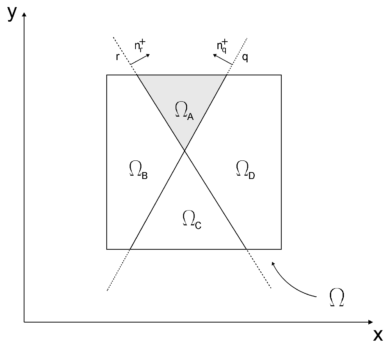
3.1. Problem Statement

Consider a body B and let u be the displacement field so that the local partition of unity (PU) approximation field referred to the set of variables x = ( x , y ) is:
u ( x ) = I n N I ( x ) ( u I + a I Ψ ( x ) )
where n is the number of nodes of the finite element mesh, N I ( x ) are the shape functions of the finite elements, Ψ ( x ) is the enrichment function and u I and a I are the standard and enriched nodal variables, respectively. Assume that d is an ensemble of m discontinuity surfaces, and let s i ( x ) be the signed distance of a point x to the i-th discontinuity surface d i . In the case of a strong discontinuity (e.g., a crack), the discontinuity in the displacement field can be described considering the standard Heaviside step function as the enrichment function Ψ  [25]:
Ψ ( x ) = H ( x ) = sign ( s i ( x ) ) = 1 if s i ( x ) 0 0 if s i ( x ) < 0
Note that, in the context of XFEM, the Heaviside enrichment component is to be applied to the nodes of the elements crossed by the discontinuity, called enriched elements [13]. Moreover, the existence of the enrichment function in (4) in the enriched elements through (3) results in the standard Gauss quadrature method for calculating the element stiffness matrix being unsuitable. As stated in Section 1, the standard approach is to divide the element domain into quadrature subdomains, which are defined by the i-th discontinuity surface d i  [13]. In the following subsections, the method to avoid domain subdivision will be deployed. In Section 3.2, the problem of a finite element cut by a strong discontinuity and the solution proposed in [13] will be illustrated. Starting from this solution, the problem of a finite element cut by two strong discontinuities is analysed and the proposed algorithm will be introduced in Section 3.3.

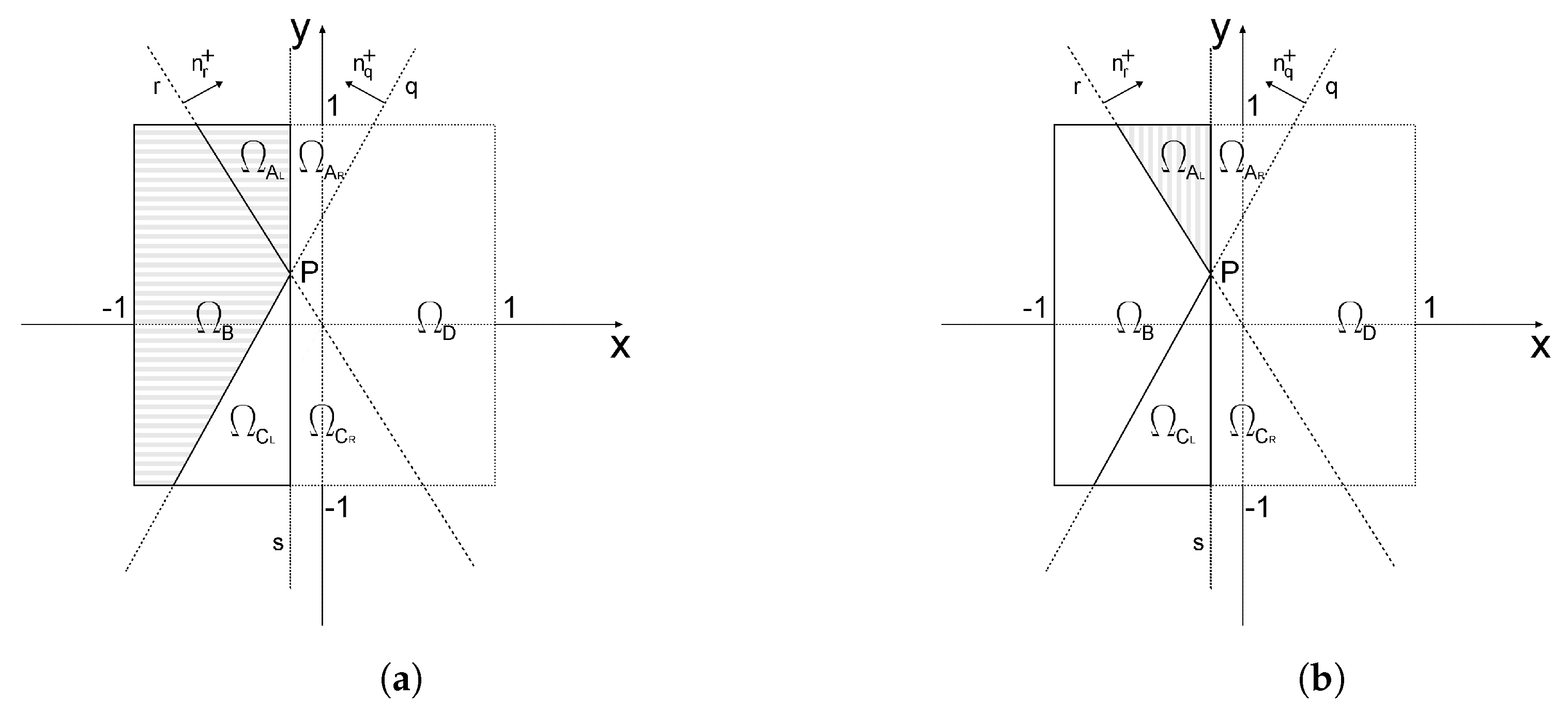
3.2. Integration Algorithm for Single Discontinuity Problems

Consider the body B described in Section 3.1. Suppose that it is meshed utilising bilinear quadrilateral finite elements, and analyse an element Ω of the mesh. Assuming that Ω is split in two parts by a discontinuity line d (defined by (5)), it is possible to define two subdomains on the two sides of the discontinuity: Ω + and Ω (Figure 1).
d : a x + b y + c = 0
The vector n+ in Figure 1 defines the positive portion of the element domain Ω and points in the direction of Ω +. The coefficients a and b in (5) for the internal discontinuity line d are used to describe the components of the vector n+, which is orthogonal to d.
The equivalent polynomial technique [13,19] allows us to map the integrand terms containing the discontinuous Heaviside function onto an equivalent polynomial with the same integral. This allows us to map the integrand onto a polynomial function, so that standard quadrature rules (e.g., Gaussian) can be applied and partitioning into subdomains is no longer required.
To describe the equivalent polynomial technique, the symbolic form of the finite element stiffness matrix is taken as a reference [13], but the general idea is that any integrand containing terms given by a polynomial times the Heaviside function can be exactly integrated by replacing the discontinuous Heaviside function with an equivalent polynomial counterpart.
With reference to a classical linear small displacement elasticity problem, the displacement and strain fields in a single enriched finite element can be written as:
u = N u Ω + Ψ Ω N a Ω
ε = B u Ω + Ψ Ω B a Ω + ( ε Ψ Ω ) N a Ω
where u Ω and a Ω are the element standard and enriched nodal variables and ε is the symmetric gradient operator, so B u Ω = ( ε N ) u Ω . E is the elastic operator, so that the stress σ is given by σ = E ε  [13]. Therefore, we consider that:
  • The strain matrix B is defined by linear functions for the bilinear quadrilateral element [13];
  • ε Ψ Ω is identically zero [13].
Then, the element stiffness matrix for the nodal variables u Ω and a Ω is given by:
K Ω = Ω k u u k u a k a u k a a d Ω = Ω B T E B H B T E B H B T E B H 2 B T E B d Ω
where the off-diagonal part H B T E B is not integrable by Gauss quadrature in the entire domain Ω  [13]. The solution proposed by Ventura [13,19] through equivalent polynomials is based on substituting the discontinuous Heaviside function H ( x ) with an equivalent polynomial function H ˜ ( x ) , continuous over the entire domain, Ω , such that [20]:
Ω H ˜ ( x ) p n ( x ) d Ω = Ω H ( x ) p n ( x ) d Ω + Ω + H ( x ) p n ( x ) d Ω
where p n ( x ) is an n-degree polynomial function to be integrated (such as B T E B in (8)).
If such polynomial H ˜ ( x ) exists, the integration can be performed on the entire domain of the element using traditional Gauss quadrature [13]. Therefore, substituting the definition of H ( x ) from (4) into (9), a polynomial function p n ( x ) can be integrated over the domain Ω + (Figure 1) through the integral:
I = Ω + p n ( x ) d Ω = Ω H ( x ) p n ( x ) d Ω = Ω H ˜ ( x ) p n ( x ) d Ω
Thus, it is no longer required to partition the domain of integration, and the integral in (10) can be evaluated over the entire domain, Ω . Based on the theory introduced in [13,19] an equivalent polynomial library called EQP has been developed by the authors [20]. This library is an effective practical tool that allows the user to evaluate integrals of polynomials times step function over various shapes of 2D and 3D domains of integration.

3.3. Integration Algorithm for Double Discontinuity Problems

The case of multiple discontinuities within the same finite element is not uncommon in the context of fracture mechanics [20], for instance when crack branching, kinking or junction occurs, both in linear and nonlinear materials [11,21,22,23,24]. Consider the body R introduced in Section 3.2 and a quadrangular element of its mesh, Ω , assuming it is divided into four portions by the discontinuity lines q and r, as illustrated in Figure 2. Define Ω A as the partition obtained when the normal to each discontinuity points inwards. Starting from Ω A , the remaining partitions ( Ω B , Ω C and Ω D ) are defined counterclockwise by convention.
The element stiffness matrix (in the context of XFEM) has to be evaluated on each of the four subdomains Ω A , Ω B , Ω C or Ω D . As seen in (8), such a matrix will contain discontinuous functions times polynomials that cannot be integrated using standard quadrature rules over the entire domain, Ω .
It should be observed that the definition of the Heaviside step function (4) is such that the integrand function is zeroed on the subdomains with negative signed distance, so that a proper definition of the discontinuities normal vectors allows us to perform the quadrature on each subdomain. This also allows straightforward extension of the method to the generalised Heaviside function, having values + 1 and 1 on the two sides of the discontinuity instead of + 1 and 0, as per definition (4).
Assume an nth-degree polynomial p n ( x ) to be integrated across the subdomains Ω A , Ω B , Ω C or Ω D obtained by partitioning a regular 2 × 2 square centred in ( 0 , 0 ) on the ( x , y ) reference system with two lines q and r, so it is:
I i = Ω i p n ( x ) d Ω
where: i = { A , B , C , D } and p n ( x ) = k 0 + k 1 x + k 2 x 2 + k 3 x y + k 4 y + k 5 y 2 +   + k m 1 x n + k m y n .
To compute the integral in (11) for each value of i with standard quadrature approaches, the definition of each integration subdomain Ω i is required. Due to the possibility of the integration domains producing rather complex polygonal shapes depending on the slope of the lines, this is not always an easy task.
The target is to use the equivalent polynomials for the two discontinuities p and r in order to allow, for each subdomain Ω i , the integration over the entire element domain Ω by means of the regular Gauss–Legendre quadrature rule, i.e., to compute (11) with integrations on the entire element domain Ω instead of Ω i .
Let H ˜ p + and H ˜ r + be the equivalent polynomials related to the normals n p + and n r + , and H ˜ p and H ˜ r be the equivalent polynomials related to the reversed normals n p + and n r + . With reference to Figure 2, we have:
I A + I D = Ω A Ω D p n ( x ) d Ω = Ω H ˜ r + ( x ) p n ( x ) d Ω
I A + I B = Ω A Ω B p n ( x ) d Ω = Ω H ˜ q + ( x ) p n ( x ) d Ω
I B + I C = Ω B Ω C p n ( x ) d Ω = Ω H ˜ r ( x ) p n ( x ) d Ω
I C + I D = Ω C Ω D p n ( x ) d Ω = Ω H ˜ q ( x ) p n ( x ) d Ω
Equations (12) to (15) give a system of four equations in the four unknowns I A , I B , I C and I D that, in general, can be proved to be indeterminate. In particular, it can be observed that if the intersection point between the two discontinuities q and r is external to the element domain or is on its boundary, then the solution will be unique. If the intersection point lies inside the element domain, the system will be indeterminate, with the system coefficient matrix having rank three.
When the intersection point between the two discontinuities q and r is internal to the element domain, the above observation suggests the introduction of an auxiliary integration limit s along the abscissa axis of the element domain to eliminate indeterminacy. The line x = s contains the discontinuities intersection point P and is parallel to the vertical axis of the reference system. It should be noted that the introduction of the auxiliary integration limit s keeps the reduced integration domain rectangular, so that standard quadrature rules can be applied.
Let H ˜ q + ( s ) ( x ) and H ˜ r + ( s ) ( x ) be the equivalent polynomial functions for the discontinuities q and r evaluated into the regular 2 × 2 square element (called the parent element), with respect to the domain bounded by s (Figure 3). Combining them together, it is possible to find the equivalent polynomial H ˜ i ( x ) :
I i = Ω i p n ( x ) d Ω = Ω H ˜ i ( x ) p n ( x ) d Ω
With reference to Figure 3, the equivalent polynomial functions to perform the integration on each of the four areas in (16) are
H ˜ A ( x ) = H ˜ q + ( x ) H ˜ B ( x )
H ˜ B ( x ) = H ˜ q + ( s ) ( x ) H ˜ r + ( s ) ( x )
H ˜ C ( x ) = H ˜ r ( x ) H ˜ B ( x )
H ˜ D ( x ) = H ˜ r + ( x ) H ˜ q + ( x ) + H ˜ B ( x )
with the equivalent polynomial functions H ˜ A ( x ) H ˜ D ( x ) representing linear combinations of equivalent polynomials for the single discontinuity lines q and r, they will depend on the equations of the two discontinuities and, according to [13,19], will have the same degree of p n ( x ) and the algebraic polynomial form:
H ˜ i ( x ) = c · m ( x )
where the vector m ( x ) gather a monomial basis, i.e., m ( x ) = ( 1 , x , y , x 2 , . . . ) , and c is a vector of coefficients [20]. Since H ˜ i ( x ) p n ( x ) is a polynomial function that is continuous over the entire domain, Ω , it can be exactly integrated with a proper quadrature rule [20]. It has to be noted that the integrand in (16) has doubled its degree, compared to the one in (11), thus slightly increasing the computational effort. The main advantage of this approach is that it allows integration over the standard domain Ω or its rectangular restriction defined by the line s, rather than the non-standard partitioned subdomains Ω A Ω D .

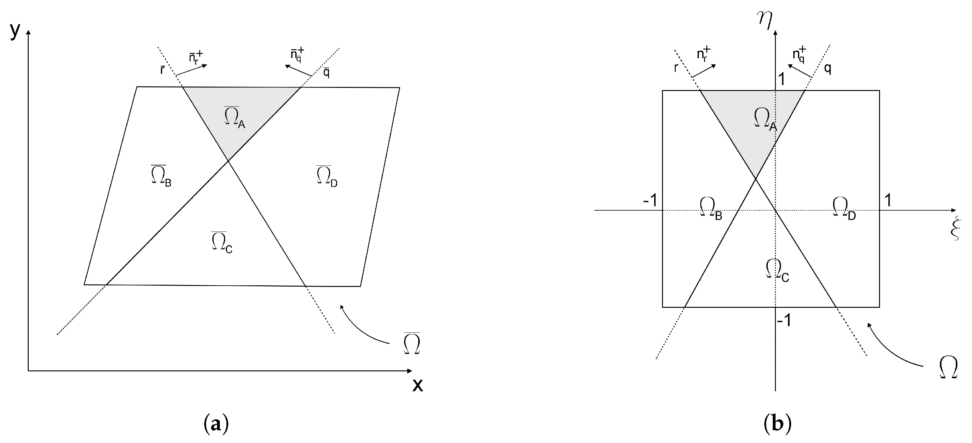
3.4. Algorithm Description

The purpose of the proposed algorithm is to deliver the expression for the equivalent polynomial function H ˜ i ( x ) , in order to compute the integral in Equation (16) without splitting the integration domain. The usefulness of the proposed algorithm is presented by way of a generic example. Let us consider a polynomial p n ( x ) to be integrated over a subdomain Ω ¯ A , generated by dividing a parallelogram Ω ¯ with two lines q ¯ and r ¯ , as shown in Figure 4a. The problem is defined in the global coordinate system x = ( x , y ) . Applying Equation (16) after the equivalent polynomial function H ˜ A ( x ) determines:
I = Ω ¯ A p n ( x ) d Ω ¯ = Ω ¯ H ˜ A ( x ) p n ( x ) d Ω ¯
Beforehand, the problem has to be mapped to a standard quadrature domain. Therefore, a change in variables from the ( x , y ) coordinate system to the parent coordinate system ( ξ , η ) is employed in order to compute the integral over a standard and regular domain, as illustrated in Figure 4b. By means of such a procedure, single parent geometry can be used to address various scenarios. Thus, parallelograms having any position and size in the global coordinate system can be mapped to the square parent geometry in the local coordinate system ( ξ , η ) [ 1 , + 1 ] illustrated in Figure 4b.
The mathematical concept used in the proposed algorithm (as well as in the DD_EQP library) for this purpose is isoparametric mapping, which is commonly employed in the FEM [9,49]. Let P ( ξ , η ) Ω be a generic point in the parent reference system, corresponding to the point P ¯ ( x , y ) Ω ¯ in the global reference system. The mapping of P ( ξ , η ) onto P ¯ ( x , y ) is described by:
x = i = 1 v N i ( ξ , η ) x i
y = i = 1 v N i ( ξ , η ) y i
where v is the number of nodes of the geometric element denoted by coordinates ( x i , y i ) in the global reference system, and N i ( ξ , η ) is the shape function in terms of local coordinates for the parent element i-th node [20].
Likewise, the discontinuities q ¯ ( x ) and r ¯ ( x ) equations, defined in the global reference system, have to be mapped onto q ( ξ ) and r ( ξ ) , defined in the parent coordinate system (Figure 4). This is achieved by:
  • Calculating the signed distances ( D i ) in the global coordinate system between each discontinuity and each node of the integration domain;
  • Writing the discontinuity coefficients (a, b and c) in the parent coordinate system as a function of D i by solving a linear equations system;
  • Substituting the variables x and y in q ¯ ( x ) and r ¯ ( x ) by means of Equation (23), so that q ( ξ ) and r ( ξ ) are obtained in terms of the coefficients a , b and c dependent on D i .
For a 2D square parent element, the coefficients are:
a = D 2 D 1 2
b = D 3 D 1 2
c = D 2 + D 3 2
After q ¯ ( x ) and r ¯ ( x ) are transformed into q ( ξ ) and r ( ξ ) , the correct expression for the equivalent polynomial function H ˜ i ( x ) with respect to the parent domain coordinate system can be generated. The coordinates and integration domain transformation in the quadrature are then introduced using the Jacobian matrix, which contains the partial derivatives of the interpolation functions N i that are differentiated with respect to the parent system variables ( ξ , η )  [76].
I = Ω ¯ H ˜ i ( x ) p n ( x ) d Ω ¯ = Ω H ˜ i ( ξ ) p n ( ξ ) | J | d Ω = = j = 1 g p w j H ˜ i ( ξ j , η j ) p n ( ξ j , η j ) | J ( ξ j , η j ) |
where | J | is the Jacobian matrix determinant. The integral in Equation (22) is calculated in (25), applying the standard scheme of the Gauss–Legendre numerical quadrature [77]. In (25), g p stands for the number of Gauss–Legendre quadrature points and w j stands for each point weight. It needs to be emphasised that the proposed algorithm is intended for integration over the entire domain Ω ¯ yielding the result of the integral over the subdomains Ω ¯ A , Ω ¯ B , Ω ¯ C and Ω ¯ D . Thus, the discontinuities equations have to be accurately defined, so that the unit vectors n i + point inwards. Additionally, it has to be noted that the discontinuities do not necessarily have to intersect Ω ¯ or one another (the proposed algorithm can handle all possible scenarios). The composition and the degree of the polynomials that can be precisely integrated using the suggested technique rely on specific requirements necessary to find the equivalent polynomial, as can be deduced from Refs. [13,19].

4. Results

The algorithm presented in Section 3.4 has been implemented into a Fortran library called double discontinuity EQP, DD_EQP, which provides the expressions of the equivalent polynomial functions H ˜ i ( x ) for 2D quadrangular integration domains as a function of the position of two discontinuity lines. In this Section, the library is used to validate the proposed algorithm and prove its robustness by means of numerical examples. The equivalent polynomial functions H ˜ i ( x ) are evaluated into a regular square parent element. More details about the mathematical formulation employed to compute the equivalent polynomial H ˜ i ( x ) for each discontinuity can be found in [13,19]. It has to be noted that the exact same procedure can be applied to a standard triangular parent element and that an extension of the proposed formulation to three-dimensional parent elements such as tetrahedrons and hexahedrons is possible, but it will not be discussed further in this paper. Moreover, in [20], the standard equivalent polynomial formulation (see Section 3.2), which is the base for the proposed algorithm, has been applied to non-polygonal element shapes such as circle or sphere parent elements. An extension of the proposed method to other non-conventional polygonal shapes can be achieved (as long as the conditions to define an equivalent polynomial for the chosen polygonal shape are met). However, since quadrangular bilinear elements are commonly employed in finite element analysis in contrast to generic polygons [9,49,76], this paper focuses on this particular element shape.
In the following subsections, the library architecture is presented and two numerical examples are carried out. The results obtained by means of the proposed algorithm are then compared with other integration methods and validated.

4.1. Library Architecture

The library source code is freely available and usable. The fundamental file of the library is dd_eqpol.f90, in which the algorithm to map the discontinuities from the global coordinate system to the parent coordinate system (retrieving their coefficients) and the algorithm to evaluate the equivalent polynomial functions H ˜ i ( x ) are contained. Other files that include the coefficients’ analytical expressions, required to evaluate the equivalent polynomial functions, complete the system. Table 1 contains a list of the monomials that the integrand polynomial function can be made up of. Nevertheless, in each of the analysed domains, the library may be extended to any polynomial degree. Note that the method provides exact results for constant Jacobian and approximate results for non-constant Jacobian [13,19].
The library is completed by the module file class_Quad.f90, which contains the 2D square finite element Class and all the methods needed to perform the element isoparametric mapping and to evaluate the integral in (25). The module file i_functions.f90, containing the methods to handle the data input via text file, is also provided. A main program file, main.f90, which implements both the library and the 2D square element Class is provided for the purpose of usage demonstration. The practical use of the library follows these steps:
  • Primary data preparation:
    • Individuation of the domain nodal coordinates in the global coordinate system;
    • Individuation of the discontinuities coefficients in the global coordinate system;
    • Selection of the domain portions to be evaluated.
  • Isoparametric mapping onto the parent element domain and computation of the coefficient vector of the equivalent polynomial by means of the DD_Heqpol_coefficients subroutine.
  • Quadrature by way of any chosen rule (i.e., (25)) in which the equivalent polynomial values at the quadrature points are provided by the function HeqPol and the Jacobian matrix determinant is given by the function detJ.
In order to obtain exact quadrature results by means of the current version of the library, the following conditions have to be met:
  • The Jacobian of the transformation in (25) has to be constant;
  • The polynomial p n in (22) is a linear combination of the monomials presented in Table 1.
It should be noted that two calls are needed if users seek to directly incorporate the core of the library into their own quadrature algorithm: one call to the subroutine Heqpol_coefficients for each integration domain (step 2, mentioned previously), and one to the function HeqPol for each quadrature point (step 3, mentioned previously). Notice that users can add their own quadrature algorithm directly into the element Class. In this case, a new method has to be defined within the element Class and a call to this method in the EvalQuad and EvalQuadFromFile subroutines has to be foreseen.

4.2. Numerical Examples

The presented examples are reproducible by means of the usage example files example_1.txt and example_2.txt provided along with the library. The results produced by the library are exact with machine precision.

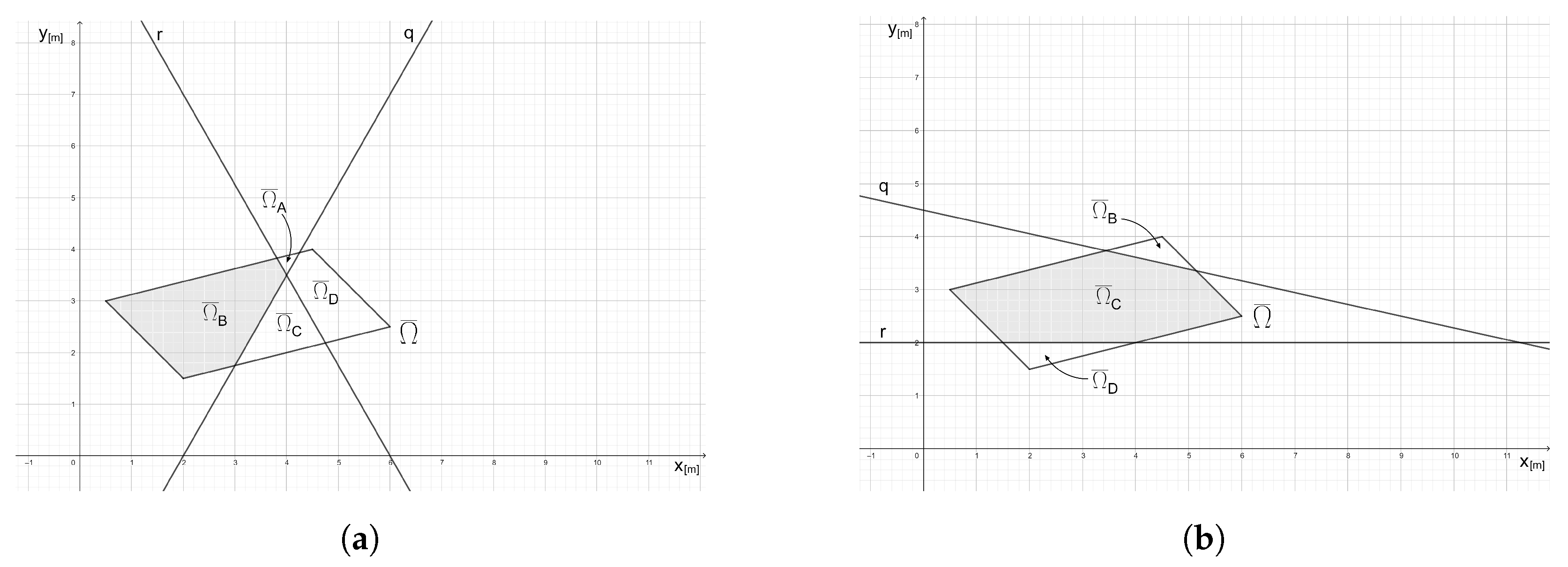
4.2.1. Parallelogram Partitioned by Two Discontinuities Intersecting within the Element

The parallelogram element Ω ¯ shown in Figure 5a as a part of a bigger body discretisation is examined in the first example. All dimensions are in meters. The element is crossed by two discontinuities, described by means of the lines q and r:
  • q : 7 4 x y 7 2 = 0 ;
  • r : 7 4 x + y 21 2 = 0 .
and split into the subdomains Ω ¯ A , Ω ¯ B , Ω ¯ C and Ω ¯ D . The objective is to evaluate the inertia tensor and the area of Ω ¯ B , namely solving the integral in (26) by means of the proposed formulation without subdividing the integration domain Ω ¯ .
Ω m ( x ) H q ( x ) H r ( x ) d Ω
where vector m ( x ) contains the monomial basis listed in Table 1 and H q ( x ) and H r ( x ) are the step functions for each discontinuity line (see (4)). Note that the normal to each discontinuity line has to be accurately defined for the sake of obtaining the targeted domain portion (as discussed in Section 3.3).
The software maps the parallelogram Ω ¯ onto the parent coordinate system, which is used to compute H ˜ B ( x ) and carry out the integration.
After launching the library example program, the user has to choose whether to input the data manually as the program executes or select an input data file.
  • Input from file? (y/n): y
  • example_1.txt
For the first example, the input data is provided by the text file example_1.txt.
  • \\ DOUBLE DISCONTINUITY EQP LIBRARY
  • \\ EXAMPLE 1: DISCONTINUITIES INTERSECTING INSIDE THE DOMAIN
  • $ElementType
  • \\ 21 : Quad
  • 21
  • $Coords
  • \\ Set the coordinates for the element
  • \\ 1st col : x
  • \\ 2nd col : y
  • \\ Coordinates Scheme :
  • \\  Quad Element :
  • \\  4-------------3
  • \\  |       |
  • \\  |       |
  • \\  |       |
  • \\  |       |
  • \\  |       |
  • \\  1-------------2
  • 2.0 1.5
  • 6.0 2.5
  • 4.5 4.0
  • 0.5 3.0
  • $NumOfDiscont
  • \\ Number of discontinuities crossing the element (1 or 2)
  • 2
  • $DiscontCoefficients
  • \\ a,b,c coefficients for each discontinuity
  • \\ coefficients are separated by a blank
  • 1.75 -1.0 -3.5
  • 1.75 1.0 -10.5
  • $ElementPart
  • \\ In case of 2 discontinuities choose the element portion
  • \\ to integrate
  • \\ Part : A, B, C, D, all
  • \\  3--------4
  • \\  | \A / |
  • \\  |B \/D |
  • \\  | / \ |
  • \\  |/ C \ |
  • \\  1--------2
  • B
where ‘ ’ identifies a comment in the input section, while ‘$’ identifies an input command.
The program creates an output file containing the integration results for all the monomials listed in Table 1, referred to as the selected domain part. The integration result for the monomial p = 1 corresponds to the area of the selected domain part, while the results for the monomials y 2 , x 2 and x , y correspond to the elements of the inertia tensor I . The results produced by the library for the area A and the inertia tensor I of Ω ¯ B , evaluated with respect to the global coordinate system ( x , y ) , are:
A = 4.371 m 2
I = ρ s 33.200 28.814 28.814 27.670 ( units : kg m 2 )
where ρ s is the material surface density ( kg / m 2 ).
In order to estimate the performance and robustness of the proposed algorithm, the integration problem has been addressed by means of the method proposed in [26] (via the integration procedure defined in [7]). The domain Ω ¯ has been split into i = 4 subdomains ( Ω ¯ A , Ω ¯ B , Ω ¯ C , Ω ¯ D ), in which the functions H q ( x ) and H r ( x ) are continuous and the integral for the portion of interest Ω ¯ B has been evaluated by means of Gauss quadrature. The integral in (26), computed above by way of the DD_EQP library, has also been evaluated numerically using the adaptive integration method “NIntegrate” of the software Wolfram Mathematica. Finally, the integration subdomain Ω ¯ B has been defined in the global reference system ( x , y ) by way of the intersections between the discontinuity lines q and r and the parallelogram domain Ω ¯ , and the definite integral at the left-hand side of Equation (16) has been exactly computed. The obtained results coincide up to machine precision for all evaluation methods, as shown in Table 2.

4.2.2. Parallelogram Partitioned by Two Discontinuities Intersecting Outside the Element

The parallelogram element Ω ¯ shown in Figure 5b as a part of a bigger body discretisation is examined in the second example. As before, all dimensions are in meters. The element is crossed by two discontinuities, described by means of the lines q and r:
  • q : 2 9 x + y 9 2 = 0 ;
  • r : y 2 = 0 .
and split into three subdomains: Ω ¯ A , Ω ¯ B and Ω ¯ C . The aim is to evaluate the inertia tensor and the area of Ω ¯ C , namely solving the integral in (26) by means of the proposed formulation, without subdividing the integration domain Ω ¯ .
The input is analogous to the previous example in Figure 5a.
The results produced by the library for the area A and the inertia tensor I of Ω ¯ C , evaluated with respect to the global coordinate system ( x , y ) , are:
A = 6.450 m 2
I = ρ s 50.817 58.396 58.396 78.392 ( units : kg m 2 )
where ρ s is the material surface density ( kg / m 2 ). As in the example in Figure 5a, the integral in (26), computed above by means of the DD_EQP library, has also been evaluated numerically by means of the method proposed in [26], via the adaptive integration strategy NIntegrate of the software Wolfram Mathematica, and by way of definite integral computation after defining the integration subdomain Ω ¯ C . Once again, the obtained results coincide to the level of machine precision for all evaluation methods, as shown in Table 2.

4.2.3. Outcomes

The outcomes of the examples presented in Section 4.2.1 and Section 4.2.2 validate both the algorithm and the DD_EQP library itself, demonstrating the robustness, precision and versatility of the proposed formulation. It has to be noted that, when equivalent polynomials are used, the integrand function doubles its degree, thus requiring a higher computational effort compared to other methods (such as in [7,25,26]) [13,19]. On the other hand, the proposed formulation removes the necessity of defining subdomains, smoothing the overall integration process.

5. Discussion

The integration algorithm presented in this paper, as well as the DD_EQP library implementing it, are helpful tools to evaluate the integral of multiple discontinuous functions by means of any numerical quadrature strategy, removing the need for dividing the domain of integration. The context for the proposed algorithm is mainly XFEM analysis of cracked bodies, in which scenarios involving crossing discontinuities are common [27,28,54,78,79,80]. Moreover, as pointed out in Section 2, the existing methods for addressing multiple discontinuities problems make use of integration strategies in which partitioning of the domain is required. The proposed algorithm is a perfect fit in this context, delivering a solution for such an issue and eliminating the need for domain splitting. It can thus potentially be adopted in many XFEM practical applications in which double discontinuities crossing the domain occur, such as hydraulic fractures and multiple cracking in rocks [81,82,83,84], brittle cracking and fracture propagation in brittle and quasi brittle materials [85,86,87], and also fracture behaviour in bones and bone-inspired bio-materials [88,89], where crack branching, junction and kinking are frequent. Nonetheless, the algorithm can be extended to various domains, such as computational geometry, where it is possible to use the library to compute the geometrical characteristics of complex figures made by cutting a simple shape (i.e., a parallelogram) using multiple lines. The proposed formulation could fit problems addressed by various authors in this field, such as in [68,72,90,91,92,93,94]. The use of both the algorithm and the library can also be extended to simulations where the objects’ shapes and locations vary dynamically, such as, for instance, an object that breaks into fragments or computer graphics in general [95,96,97,98]. Thus, the effectiveness of the presented algorithm and the simplicity of the use of the library and its ease of implementation into any computational framework make them well-suited means for a broad variety of potential applications, since numerical integration of polynomial functions with jump discontinuities is a frequent problem in various fields [16,55,56,99,100,101,102,103,104,105,106,107,108,109,110,111]. However, it has to be noted that the use of equivalent polynomials leads to a higher computational effort during quadrature than splitting the integration domain since the integrand function doubles its degree [13,19]. This aspect can be particularly burdensome in analyses containing numerous enriched elements. The optimisation and acceleration of the computation process could be possible improvements. Future developments for the proposed formulation include the capability of handling an arbitrary number of discontinuities and the extension of the presented formulation to other domain shapes, both 2D and 3D (such as triangular, tetrahedral and hexahedral elements). Finally, the implementation of the proposed algorithm into computational frameworks for practical use on a larger scale in the context of fracture mechanics and computational geometry may also be addressed.

6. Conclusions

The integration of polynomials times double step functions within quadrilateral domains has been explored in this paper. The study focused on investigating the behaviour and properties of these integrals and their applications in various fields, especially XFEM analysis. The integration of polynomials times double step functions within quadrilateral domains represents a challenging task, mainly due to the piecewise nature of the double step functions. However, an integration algorithm to effectively perform these integrations by means of equivalent polynomials has been developed and presented in this paper, along with a software library for its implementation. Both the library and the presented algorithm are ready-to-use handy tools for numerically computing integrals of polynomial functions across generic subdomains generated by two discontinuities partitioning a regular integration domain. In this paper, two practical numerical examples of the library usage have been carried out, and the results demonstrated the ease of calculation, the removal of complicated subdomain processing and the absolute accuracy of the proposed algorithm. Moreover, a comparison with other integration methods for the same numerical examples has been carried out and validated the proposed formulation. In addition, the utter generality and extensibility of the mathematical framework that underlies the library and the proposed formulation are among their key points. Furthermore, in addition to XFEM analysis in the context of fracture mechanics, the integration of polynomials times double step functions in quadrilateral domains exhibited promising applications in various fields, such as numerical simulations, computational geometry and engineering problems that involve modelling phenomena with sharp transitions or abrupt changes. The capability to accurately integrate such functions within quadrilateral domains without subdividing the integration domain could define pathways for more precise calculations in these contexts. Future research can further explore advanced numerical techniques and optimisation approaches to improve the efficiency and accuracy and enable the possibility of taking into account an arbitrary number of discontinuities.

Supplementary Materials

The following supporting information can be downloaded at: https://www.mdpi.com/article/10.3390/a16060290/s1, The source code of the DD_EQP Fortran library embedding the proposed integration algorithm, as well as the numerical examples used in this paper and software documentation, can be found at: equivalent-polynomials.net (https://sites.google.com/view/eqpols accessed on 1 March 2023). A maintained GitHub repository (https://github.com/sebfichera/DD_EQP_Library accessed on 1 March 2023) for the DD_EQP library is also available.

Author Contributions

Conceptualisation, G.V. and M.C.; methodology, M.C., G.M. and S.F.; software, S.F. and G.M.; validation, S.F., G.M. and M.C.; formal analysis, S.F. and G.M.; investigation, S.F. and G.M.; resources, G.V. and M.C.; data curation, S.F. and G.M.; writing—original draft preparation, S.F., G.M., M.C. and G.V.; writing—review and editing, S.F., G.M., M.C. and G.V.; visualisation, S.F. and G.M.; supervision, G.V. and M.C. All authors have read and agreed to the published version of the manuscript.

Funding

Ministry of University and Research (MUR), research project XFAST-SIMS: Extra fast and accurate simulation of complex structural systems (Grant agreement n. 20173C478N) partially funded this research.

Data Availability Statement

No new data were created or analysed in this study. Data sharing is not applicable to this article.

Acknowledgments

Research support by Politecnico di Torino with the diffuse research grant initiative is gratefully acknowledged.

Conflicts of Interest

The authors declare no conflict of interest: we wish to confirm that there are no known conflict of interest associated with this publication and there has been no significant financial support for this work that could have influenced its outcome.

Abbreviations

The following abbreviations are used in this manuscript:
MDPIMultidisciplinary Digital Publishing Institute
FEMFinite element method
PUMPartition of unity method
CZMCohesive zone model
BEMBoundary element method
SBFEMScaled boundary finite element method
SPHSmoothed particle hydrodynamics
RKPMReproducing kernel particle method
XFEMExtended finite element method
GFEMGeneralised finite element method
EQPEquivalent polynomials
DD_EQPDouble discontinuity equivalent polynomials

References

  1. Hughes, T. The Finite Element Method: Linear Static and Dynamic Finite Element Analysis; Dover Publications: Mineola, NY, USA, 2000. [Google Scholar]
  2. Babuška, I.; Suri, M. The p-version of the finite element method. SIAM J. Numer. Anal. 1992, 29, 864–893. [Google Scholar] [CrossRef]
  3. Belytschko, T.; Lu, Y.; Gu, L. Element-free Galerkin methods. Int. J. Numer. Methods Eng. 1994, 37, 229–256. [Google Scholar] [CrossRef]
  4. Duarte, C.; Babuška, I.; Oden, J. Generalized finite element method for three-dimensional structural mechanics problems. Comput. Struct 2000, 77, 219–232. [Google Scholar] [CrossRef] [Green Version]
  5. Melenk, J.; Babuška, I. The partition of unity finite element method: Basic theory and applications. Comput. Methods Appl. Mech. Eng. 1996, 139, 289–314. [Google Scholar] [CrossRef] [Green Version]
  6. Sukumar, N.; Moran, B. Extended finite element method for three-dimensional crack modelling. Int. J. Numer. Methods Eng. 1998, 43, 847–884. [Google Scholar] [CrossRef]
  7. Moës, N.; Dolbow, J.; Belytschko, T. A finite element method for crack growth without remeshing. Int. J. Numer. Methods Eng. 1999, 46, 131–150. [Google Scholar] [CrossRef]
  8. Fries, T.; Belytschko, T. The extended/generalized finite element method: An overview of the method and its applications. Int. J. Numer. Methods Eng. 2010, 84, 253–304. [Google Scholar] [CrossRef]
  9. Bathe, K.J. Finite Element Procedures, 2nd ed.; Klaus-Jürgen Bathe: Watertown, MA, USA, 2014. [Google Scholar]
  10. Belytschko, T.; Liu, W.K.; Moran, B.; Elkhodary, K. Nonlinear Finite Elements for Continua and Structures, 2nd ed.; Wiley: Chichester, UK, 2014. [Google Scholar]
  11. Rabczuk, T.; Song, J.H.; Zhuang, X.; Anitescu, C. Extended Finite Element and Meshfree Methods; Academic Press: London, UK, 2019. [Google Scholar]
  12. Belytschko, T.; Gracie, R.; Ventura, G. A review of extended/generalized finite element methods for material modeling. Model. Simul. Mater. Sci. Eng. 2009, 17, 1–24. [Google Scholar] [CrossRef]
  13. Ventura, G. On the elimination of quadrature subcells for discontinuous functions in the eXtended Finite-Element Method. Int. J. Numer. Meth. Eng. 2006, 66, 761–795. [Google Scholar] [CrossRef]
  14. Belytschko, T.; Black, T. Elastic crack growth in finite elements with minimal remeshing. Int. J. Numer. Meth. Eng. 1999, 45, 601–620. [Google Scholar] [CrossRef]
  15. Mousavi, S.; Pask, J.; Sukumar, N. Efficient adaptive integration of functions with sharp gradients and cusps in n-dimensional parallelepipeds. Int. J. Numer. Methods Eng. 2012, 91, 343–357. [Google Scholar] [CrossRef] [Green Version]
  16. Chin, E.; Lasserre, J.; Sukumar, N. Modeling crack discontinuities without element-partitioning in the extended finite element method. Int. J. Numer. Methods Eng. 2017, 110, 1021–1048. [Google Scholar] [CrossRef]
  17. Benvenuti, E.; Tralli, A.; Ventura, G. A regularized XFEM model for the transition from continuous to discontinuous displacements. Int. J. Numer. Methods Eng. 2008, 74, 911–944. [Google Scholar] [CrossRef]
  18. Benvenuti, E.; Ventura, G.; Ponara, N. Finite element quadrature of regularized discontinuous and singular level set functions in 3D problems. Algorithms 2012, 5, 529–544. [Google Scholar] [CrossRef] [Green Version]
  19. Ventura, G.; Benvenuti, E. Equivalent polynomials for quadrature in Heaviside function enriched elements. Int. J. Numer. Methods Eng. 2015, 102, 688–710. [Google Scholar] [CrossRef]
  20. Mariggiò, G.; Fichera, S.; Corrado, M.; Ventura, G. EQP - A 2D/3D library for integration of polynomials times step function. SoftwareX 2020, 12, 100636. [Google Scholar] [CrossRef]
  21. Ha, K.; Baek, H.; Park, K. Convergence of fracture process zone size in cohesive zone modeling. Appl. Math. Model. 2015, 39, 5828–5836. [Google Scholar] [CrossRef]
  22. Bordas, S.; Rabczuk, T.; Zi, G. Three-dimensional crack initiation, propagation, branching and junction in non-linear materials by an extended meshfree method without asymptotic enrichment. Eng. Fract. Mech. 2008, 75, 943–960. [Google Scholar] [CrossRef] [Green Version]
  23. Rabczuk, T.; Zi, G.; Bordas, S.; Nguyen-Xuan, H. A simple and robust three-dimensional cracking-particle method without enrichment. Comput. Methods Appl. Mech. Eng. 2010, 199, 2437–2455. [Google Scholar] [CrossRef]
  24. Rabczuk, T.; Bordas, S.; Zi, G. A three-dimensional meshfree method for continuous multiple-crack initiation, propagation and junction in statics and dynamics. Comput. Mech. 2007, 40, 473–495. [Google Scholar] [CrossRef] [Green Version]
  25. Belytschko, T.; Moës, N.; Usui, S.; Parimi, C. Arbitrary discontinuities in finite elements. Int. J. Numer. Methods Eng. 2001, 50, 993–1013. [Google Scholar] [CrossRef]
  26. Daux, C.; Moës, N.; Dolbow, J.; Sukumar, N.; Belytschko, T. Arbitrary branched and intersecting cracks with the extended finite element method. Int. J. Numer. Methods Eng. 2000, 48, 1741–1760. [Google Scholar] [CrossRef]
  27. Singh, I.V.; Bhardwaj, G.; Mishra, B. A new criterion for modeling multiple discontinuities passing through an element using XIGA. J. Mech. Sci. Technol. 2015, 29, 1131. [Google Scholar] [CrossRef]
  28. Wen, L.F.; Tian, R.; Wang, L.X.; Feng, C. Improved XFEM for multiple crack analysis: Accurate and efficient implementations for stress intensity factors. Comput. Methods Appl. Mech. Eng. 2023, 411, 116045. [Google Scholar] [CrossRef]
  29. Khoei, A.R. Extended Finite Element Method: Theory and Applications; John Wiley & Sons: Chichester, UK, 2015. [Google Scholar]
  30. Rege, K.; Lemu, H. A review of fatigue crack propagation modelling techniques using FEM and XFEM. In Proceedings of the IOP Conference Series: Materials Science and Engineering; IOP Publishing: Bristol, UK, 2017; Volume 276, p. 012027. [Google Scholar]
  31. Barenblatt, G.I. The mathematical theory of equilibrium cracks in brittle fracture. Adv. Appl. Mech. 1962, 7, 55–129. [Google Scholar]
  32. Dugdale, D.S. Yielding of steel sheets containing slits. J. Mech. Phys. Solids 1960, 8, 100–104. [Google Scholar] [CrossRef]
  33. Lachat, J.; Watson, J. Effective numerical treatment of boundary integral equations: A formulation for three-dimensional elastostatics. Int. J. Numer. Methods Eng. 1976, 10, 991–1005. [Google Scholar] [CrossRef]
  34. Xie, D.; Waas, A.M. Discrete cohesive zone model for mixed-mode fracture using finite element analysis. Eng. Fract. Mech. 2006, 73, 1783–1796. [Google Scholar] [CrossRef]
  35. Chen, Z.; Bunger, A.; Zhang, X.; Jeffrey, R.G. Cohesive zone finite element-based modeling of hydraulic fractures. Acta Mechanica Solida Sinica 2009, 22, 443–452. [Google Scholar] [CrossRef]
  36. de Borst, R.; Remmers, J.J.; Needleman, A. Mesh-independent discrete numerical representations of cohesive-zone models. Eng. Fract. Mech. 2006, 73, 160–177. [Google Scholar] [CrossRef]
  37. Alrayes, O.; Könke, C.; Hamdia, K.M. A Numerical Study of Crack Mixed Mode Model in Concrete Material Subjected to Cyclic Loading. Materials 2023, 16, 1916. [Google Scholar] [CrossRef] [PubMed]
  38. Alrayes, O.; Könke, C.; Ooi, E.T.; Hamdia, K.M. Modeling Cyclic Crack Propagation in Concrete Using the Scaled Boundary Finite Element Method Coupled with the Cumulative Damage-Plasticity Constitutive Law. Materials 2023, 16, 863. [Google Scholar] [CrossRef] [PubMed]
  39. Rabczuk, T.; Bordas, S.; Zi, G. On three-dimensional modelling of crack growth using partition of unity methods. Comput. Struct. 2010, 88, 1391–1411. [Google Scholar] [CrossRef]
  40. Liu, G. An overview on meshfree methods: For computational solid mechanics. Int. J. Comput. Methods 2016, 13, 1630001. [Google Scholar] [CrossRef]
  41. Babuška, I.; Melenk, J.M. The partition of unity method. Int. J. Numer. Methods Eng. 1997, 40, 727–758. [Google Scholar] [CrossRef]
  42. Strouboulis, T.; Babuška, I.; Copps, K. The design and analysis of the generalized finite element method. Comput. Methods Appl. Mech. Eng. 2000, 181, 43–69. [Google Scholar] [CrossRef]
  43. Strouboulis, T.; Copps, K.; Babuška, I. The generalized finite element method. Comput. Methods Appl. Mech. Eng. 2001, 190, 4081–4193. [Google Scholar] [CrossRef]
  44. Daxini, S.; Prajapati, J. A review on recent contribution of meshfree methods to structure and fracture mechanics applications. Sci. World J. 2014, 2014, 247172. [Google Scholar] [CrossRef] [Green Version]
  45. Li, S.; Liu, W.K. Meshfree and particle methods and their applications. Appl. Mech. Rev. 2002, 55, 1–34. [Google Scholar] [CrossRef] [Green Version]
  46. Liew, K.M.; Zhao, X.; Ferreira, A.J. A review of meshless methods for laminated and functionally graded plates and shells. Compos. Struct. 2011, 93, 2031–2041. [Google Scholar] [CrossRef]
  47. Rabczuk, T.; Zi, G. A meshfree method based on the local partition of unity for cohesive cracks. Comput. Mech. 2007, 39, 743–760. [Google Scholar] [CrossRef]
  48. Zi, G.; Rabczuk, T.; Wall, W. Extended meshfree methods without branch enrichment for cohesive cracks. Comput. Mech. 2007, 40, 367–382. [Google Scholar] [CrossRef] [Green Version]
  49. Zienkiewicz, O.C.; Taylor, R.L.; Zhu, J.Z. The Finite Element Method: Its Basis and Fundamentals, 6th ed.; Butterworth-Heinemann: Oxford, UK, 2005. [Google Scholar]
  50. Babuška, I. The rate of convergence for the finite element method. SIAM J. Numer. Anal. 1971, 8, 304–315. [Google Scholar] [CrossRef]
  51. Ciarlet, P.G. The Finite Element Method for Elliptic Problems; SIAM: Philadelphia, PA, USA, 2002. [Google Scholar]
  52. Li, D.; Liu, J.H.; Nie, F.H.; Featherston, C.A.; Wu, Z. On tracking arbitrary crack path with complex variable meshless methods. Comput. Methods Appl. Mech. Eng. 2022, 399, 115402. [Google Scholar] [CrossRef]
  53. Garg, S.; Pant, M. Meshfree methods: A comprehensive review of applications. Int. J. Comput. Methods 2018, 15, 1830001. [Google Scholar] [CrossRef]
  54. Oren, I. Admissible functions with multiple discontinuities. Isr. J. Math. 1982, 42, 353–360. [Google Scholar] [CrossRef]
  55. Agathos, K.; Chatzi, E.; Bordas, S.P. Multiple crack detection in 3D using a stable XFEM and global optimization. Comput. Mech. 2018, 62, 835–852. [Google Scholar] [CrossRef] [Green Version]
  56. Mousavi, S.; Sukumar, N. Numerical integration of polynomials and discontinuous functions on irregular convex polygons and polyhedrons. Comput. Mech. 2011, 47, 535–554. [Google Scholar] [CrossRef] [Green Version]
  57. Fichera, S.; Biondi, B.; Ventura, G. 2D finite elements for the computational analysis of crack propagation in brittle materials and the handling of double discontinuities. Procedia Struct. Integr. 2022, 42, 1291–1298. [Google Scholar] [CrossRef]
  58. Fichera, S.; Biondi, B.; Ventura, G. Implementation into OpenSees of XFEM for Analysis of Crack Propagation in Brittle Materials. In Proceedings of the 2022 Eurasian OpenSees Days; Springer: Berlin/Heidelberg, Germany, 2023; pp. 157–165. [Google Scholar]
  59. Mariggiò, G.; Ventura, G.; Corrado, M. A probabilistic FEM approach for the structural design of glass components. Eng. Fract. Mech. 2023, 282, 109157. [Google Scholar] [CrossRef]
  60. Bender, J.; Erleben, K.; Trinkle, J. Interactive simulation of rigid body dynamics in computer graphics. Comput Graph Forum. 2014, 33, 246–270. [Google Scholar] [CrossRef]
  61. Machenhauer, B.; Kaas, E.; Lauritzen, P.H. Finite-Volume Methods in Meteorology. In Proceedings of the Computational Methods for the Atmosphere and the Oceans; Temam, R.M., Tribbia, J.J., Eds.; Elsevier Science: Amsterdam, The Netherlands, 2008; pp. 1–120. [Google Scholar]
  62. Timmer, H.; Stern, J. Computation of global geometric properties of solid objects. Comput.-Aided Des. 1980, 12, 301–304. [Google Scholar] [CrossRef]
  63. Krishnamurthy, A.; McMains, S. Accurate GPU-accelerated surface integrals for moment computation. Comput.-Aided Des. 2011, 43, 1284–1295. [Google Scholar] [CrossRef]
  64. Mamatha, T.; Venkatesh, B. Gauss quadrature rules for numerical integration over a standard tetrahedral element by decomposing into hexahedral elements. Appl. Math. Comput. 2015, 271, 1062–1070. [Google Scholar] [CrossRef]
  65. Chin, E.B.; Sukumar, N. An efficient method to integrate polynomials over polytopes and curved solids. Comput. Aided Geom. Des. 2020, 82, 101914. [Google Scholar] [CrossRef]
  66. Saye, R. High-order quadrature methods for implicitly defined surfaces and volumes in hyperrectangles. SIAM J. Sci. Comput. 2015, 37, A993–A1019. [Google Scholar] [CrossRef]
  67. Farrington, C.C. Numerical quadrature of discontinuous functions. In Proceedings of the 1961 16th ACM National Meeting; Association for Computing Machinery: New York, NY, USA, 1961; pp. 21–401. [Google Scholar]
  68. Hubrich, S.; Di Stolfo, P.; Kudela, L.; Kollmannsberger, S.; Rank, E.; Schröder, A.; Düster, A. Numerical integration of discontinuous functions: Moment fitting and smart octree. Comput. Mech. 2017, 60, 863–881. [Google Scholar] [CrossRef]
  69. Tornberg, A.K. Multi-dimensional quadrature of singular and discontinuous functions. BIT Numer. Math. 2002, 42, 644–669. [Google Scholar] [CrossRef]
  70. Dai, N.; Zhang, B.; Lu, D.; Chen, Y. High-degree discontinuous finite element discrete quadrature sets for the Boltzmann transport equation. Prog. Nucl. Energy 2022, 153, 104403. [Google Scholar] [CrossRef]
  71. Mousavi, S.; Sukumar, N. Generalized Gaussian quadrature rules for discontinuities and crack singularities in the extended finite element method. Comput. Methods Appl. Mech. Eng. 2010, 199, 3237–3249. [Google Scholar] [CrossRef] [Green Version]
  72. Pali, E.; Gravouil, A.; Tanguy, A.; Landru, D.; Kononchuk, O. Three-dimensional X-FEM modeling of crack coalescence phenomena in the Smart CutTM technology. Finite Elem. Anal. Des. 2023, 213, 103839. [Google Scholar] [CrossRef]
  73. Song, C.; Zhang, H.; Wu, Y.; Bao, H. Cutting and Fracturing Models without Remeshing. In Proceedings of the Advances in Geometric Modeling and Processing; Chen, F., Jüttler, B., Eds.; Springer: Berlin/Heidelberg, Germany, 2008; pp. 107–118. [Google Scholar]
  74. Iben, H.N.; O’Brien, J.F. Generating Surface Crack Patterns. Graph Models 2009, 71, 198–208. [Google Scholar] [CrossRef] [Green Version]
  75. da Rosa Rodriguez, E.; Rossi, R. Assessment of EqP in XFEM for weak discontinuities. J. Braz. Soc. Mech. Sci. Eng. 2023, 45, 312. [Google Scholar] [CrossRef]
  76. Amazigo, J.; Rubenfeld, L. Advanced Calculus and its Application to the Engineering and Physical Science; John Wiley & Sons Inc.: Hoboken, NJ, USA, 1980. [Google Scholar]
  77. Davis, P.J.; Rabinowitz, P. Methods of Numerical Integration, 2nd ed.; Academic Press: Cambridge, MA, USA, 1984. [Google Scholar]
  78. Napier, J. Energy changes in a rockmass containing multiple discontinuities. J. South. Afr. Inst. Min. Metall. 1991, 91, 145–157. [Google Scholar]
  79. Sekhar, A. Multiple cracks effects and identification. Mech. Syst. Signal Process. 2008, 22, 845–878. [Google Scholar] [CrossRef]
  80. Kamaya, M. A crack growth evaluation method for interacting multiple cracks. Jsme Int. J. Ser. Solid Mech. Mater. Eng. 2003, 46, 15–23. [Google Scholar] [CrossRef] [Green Version]
  81. Escobar, R.G.; Sanchez, E.C.M.; Roehl, D.; Romanel, C. Xfem modeling of stress shadowing in multiple hydraulic fractures in multi-layered formations. J. Nat. Gas Sci. Eng. 2019, 70, 102950. [Google Scholar] [CrossRef]
  82. Wang, Y.; Javadi, A.A.; Fidelibus, C. A hydro-mechanically-coupled XFEM model for the injection-induced evolution of multiple fractures. Int. J. Numer. Anal. Methods Geomech. 2023. [Google Scholar] [CrossRef]
  83. Cruz, F.; Roehl, D.; do Amaral Vargas, E., Jr. An XFEM element to model intersections between hydraulic and natural fractures in porous rocks. Int. J. Rock Mech. Min. Sci. 2018, 112, 385–397. [Google Scholar] [CrossRef] [Green Version]
  84. Wang, T.; Liu, Z.; Zeng, Q.; Gao, Y.; Zhuang, Z. XFEM modeling of hydraulic fracture in porous rocks with natural fractures. Sci. China Physics Mech. Astron. 2017, 60, 1–15. [Google Scholar] [CrossRef]
  85. Liu, S.; Fang, G.; Liang, J.; Lv, D. A coupling model of XFEM/peridynamics for 2D dynamic crack propagation and branching problems. Theor. Appl. Fract. Mech. 2020, 108, 102573. [Google Scholar] [CrossRef]
  86. Richardson, C.L.; Hegemann, J.; Sifakis, E.; Hellrung, J.; Teran, J.M. An XFEM method for modeling geometrically elaborate crack propagation in brittle materials. Int. J. Numer. Methods Eng. 2011, 88, 1042–1065. [Google Scholar] [CrossRef]
  87. Gebhardt, C.; Kaliske, M. An XFEM-approach to model brittle failure of wood. Eng. Struct. 2020, 212, 110236. [Google Scholar] [CrossRef]
  88. Idkaidek, A.; Jasiuk, I. Cortical bone fracture analysis using XFEM–case study. Int. J. Numer. Methods Biomed. Eng. 2017, 33, e2809. [Google Scholar] [CrossRef]
  89. Vellwock, A.E.; Vergani, L.; Libonati, F. A multiscale XFEM approach to investigate the fracture behavior of bio-inspired composite materials. Compos. Part Eng. 2018, 141, 258–264. [Google Scholar] [CrossRef] [Green Version]
  90. Joulaian, M.; Hubrich, S.; Düster, A. Numerical integration of discontinuities on arbitrary domains based on moment fitting. Comput. Mech. 2016, 57, 979–999. [Google Scholar] [CrossRef]
  91. Abedian, A.; Düster, A. Equivalent Legendre polynomials: Numerical integration of discontinuous functions in the finite element methods. Comput. Methods Appl. Mech. Eng. 2019, 343, 690–720. [Google Scholar] [CrossRef]
  92. Lin, J.S. A mesh-based partition of unity method for discontinuity modeling. Comput. Methods Appl. Mech. Eng. 2003, 192, 1515–1532. [Google Scholar] [CrossRef]
  93. Abedian, A.; Parvizian, J.; Düster, A.; Khademyzadeh, H.; Rank, E. Performance of different integration schemes in facing discontinuities in the finite cell method. Int. J. Comput. Methods 2013, 10, 1350002. [Google Scholar] [CrossRef]
  94. You, H.; Kim, C. Direct reconstruction method for discontinuous Galerkin methods on higher-order mixed-curved meshes II. Surface integration. J. Comput. Phys. 2020, 416, 109514. [Google Scholar] [CrossRef]
  95. Smith, J.; Witkin, A.; Baraff, D. Fast and controllable simulation of the shattering of brittle objects. In Proceedings of the Computer Graphics Forum; Wiley Online Library: Oxford, UK; Boston, MA, USA, 2001; Volume 20, pp. 81–91. [Google Scholar]
  96. Norton, A.; Turk, G.; Bacon, B.; Gerth, J.; Sweeney, P. Animation of fracture by physical modeling. Vis. Comput. 1991, 7, 210–219. [Google Scholar] [CrossRef]
  97. O’brien, J.F.; Hodgins, J.K. Graphical modeling and animation of brittle fracture. In Proceedings of the 26th Annual Conference on Computer Graphics and Interactive Techniques, Los Angeles, CA, USA, 8–13 August 1999; pp. 137–146. [Google Scholar]
  98. Martin-Bragado, I.; Rivera, A.; Valles, G.; Gomez-Selles, J.L.; Caturla, M.J. MMonCa: An Object Kinetic Monte Carlo simulator for damage irradiation evolution and defect diffusion. Comput. Phys. Commun. 2013, 184, 2703–2710. [Google Scholar] [CrossRef] [Green Version]
  99. Lv, J.H.; Jiao, Y.Y.; Rabczuk, T.; Zhuang, X.Y.; Feng, X.T.; Tan, F. A general algorithm for numerical integration of three-dimensional crack singularities in PU-based numerical methods. Comput. Methods Appl. Mech. Eng. 2020, 363, 112908. [Google Scholar] [CrossRef]
  100. Düster, A.; Allix, O. Selective enrichment of moment fitting and application to cut finite elements and cells. Comput. Mech. 2020, 65, 429–450. [Google Scholar] [CrossRef]
  101. Ali, T.; Mostefa, B.; Abdelkader, D.; Abdelkrim, A.; Habibe, K. Experimental and numerical fracture modeling using XFEM of aluminum plates. Int. J. Eng. Res. Afr. 2020, 46, 45–52. [Google Scholar]
  102. Surendran, M.; Natarajan, S.; Palani, G.; Bordas, S. Linear smoothed extended finite element method for fatigue crack growth simulations. Eng. Fract. Mech. 2019, 206, 551–564. [Google Scholar] [CrossRef]
  103. Elguedj, T.; Jan, Y.; Combescure, A.; Leblé, B.; Barras, G. X-FEM Analysis of dynamic crack growth under transient loading in thick shells. Int. J. Impact Eng. 2018, 122, 228–250. [Google Scholar] [CrossRef]
  104. Müller, B.; Krämer-Eis, S.; Kummer, F.; Oberlack, M. A high-order discontinuous Galerkin method for compressible flows with immersed boundaries. Int. J. Numer. Methods Eng. 2017, 110, 3–30. [Google Scholar] [CrossRef]
  105. Sudhakar, Y.; Moitinho de Almeida, J.; Wall, W. An accurate, robust, and easy-to-implement method for integration over arbitrary polyhedra: Application to embedded interface methods. J. Comput. Phys. 2014, 273, 393–415. [Google Scholar] [CrossRef]
  106. Antonietti, P.; Verani, M.; Vergara, C.; Zonca, S. Numerical solution of fluid-structure interaction problems by means of a high order Discontinuous Galerkin method on polygonal grids. Finite Elem. Anal. Des. 2019, 159, 1–14. [Google Scholar] [CrossRef]
  107. Wu, J.Y.; Qiu, J.F.; Nguyen, V.; Mandal, T.; Zhuang, L.J. Computational modeling of localized failure in solids: XFEM vs. PF-CZM. Comput. Methods Appl. Mech. Eng. 2019, 345, 618–643. [Google Scholar] [CrossRef]
  108. Martin, A.; Esnault, J.B.; Massin, P. About the use of standard integration schemes for X-FEM in solid mechanics plasticity. Comput. Methods Appl. Mech. Eng. 2015, 283, 551–572. [Google Scholar] [CrossRef]
  109. Benvenuti, E. XFEM with equivalent eigenstrain for matrix-inclusion interfaces. Comput. Mech. 2014, 53, 893–908. [Google Scholar] [CrossRef]
  110. Formaggia, L.; Vergara, C.; Zonca, S. Unfitted extended finite elements for composite grids. Comput. Math. Appl. 2018, 76, 893–904. [Google Scholar] [CrossRef]
  111. Kudela, L.; Zander, N.; Kollmannsberger, S.; Rank, E. Smart octrees: Accurately integrating discontinuous functions in 3D. Comput. Methods Appl. Mech. Eng. 2016, 306, 406–426. [Google Scholar] [CrossRef]
Figure 1. A 2D quadrangular domain Ω crossed by a discontinuity line d.
Algorithms 16 00290 g001
Figure 2. A 2D quadrangular domain Ω crossed by two discontinuity lines: q and r.
Algorithms 16 00290 g002
Figure 3. Use of the auxiliary integration limit s to evaluate the equivalent polynomials H ˜ i ( x ) . In the figure H ˜ B ( x ) = H ˜ q + ( s ) ( x ) H ˜ r + ( s ) ( x ) . (a) Integration domain evaluated by means of H ˜ q + ( x ) with respect to the discontinuity q and the auxiliary integration limit s. (b) Integration domain evaluated by means of H ˜ r + ( x ) with respect to the discontinuity r and the auxiliary integration limit s.
Algorithms 16 00290 g003
Figure 4. Isoparametric mapping of a quadrangular element. (a) Element configuration in the global coordinate system. (b) Element configuration in the parent coordinate system.
Algorithms 16 00290 g004
Figure 5. Software illustrative examples. (a) Example 1: parallelogram domain cut by two discontinuities intersecting inside the domain. (b) Example 2: parallelogram domain cut by two discontinuities intersecting outside the domain.
Algorithms 16 00290 g005
Table 1. Integration domain, domain type, parent element domain and monomial basis included in the library.
Domain of IntegrationEtypeParent DomainMonomial Basis
Parallelogram21Algorithms 16 00290 i001 1 , x , x 2 , y , x y , y 2
Table 2. Proposed algorithm error compared to other integration methods.
Integration MethodError %
Domain splitting method ([7,26]) 0.0 %
NIntegrate adaptive integration method 0.0 %
Definite integral Equation (16) computation 0.0 %
Disclaimer/Publisher’s Note: The statements, opinions and data contained in all publications are solely those of the individual author(s) and contributor(s) and not of MDPI and/or the editor(s). MDPI and/or the editor(s) disclaim responsibility for any injury to people or property resulting from any ideas, methods, instructions or products referred to in the content.

