1. Introduction
The Dynamic Shortest Path (DSP) problem plays an important role in many real-world situations in which the environment, typically represented as a graph, is subject to updates on its topology. DSP problems appear in a wide variety of application contexts and configurations, including logistics, telecommunications, and trip planning [
1]. DSP algorithms become useful in several situations. For instance, in the case of trip planning, dynamic real-time traffic conditions (e.g., accidents) can be modeled as changes in the graph topology, which may be easier to handle than simply recomputing the desired path from scratch. However, the literature on DSP typically approaches the problem as having a single objective (e.g., travel time, in the case of trip planning), which does not always resemble how these problems are approached in the real world.
In scenarios where more than one objective needs to be considered when composing the solution, the relationship between these objectives needs to be carefully taken into account. In this scenario, the Multi-Objective Decision-Making (MODM) problem plays a fundamental role in searching for the best result, considering the trade-off between the objectives and the preferences of the user or the system. MODM problems emerge in several real-life situations, such as the economic market, pathfinding, and project definitions [
2]. However, applying MODM in the shortest path problem has been treated in the literature in the static form, also known as the Multi-Objective Shortest Path (MOSP) problem.
MOSP algorithms are unsuitable for solving the DSP problem, as any real-time update on the graph forwards the recalculation of the solution from scratch. Some works solve this problem by applying the MOSP with a time-dependent approach if the problem can be modeled with graph changes following a pattern. However, in a time-dependent MOSP problem, the variation in the values of the objectives is linked to time and conditions well-known a priori, such as rush hour on a highway. In this way, the time-dependent MOSP problem also does not allow real-time updates or unmapped conditions a priori without recomputing the entire solution from scratch. Therefore, the approaches to MOSP problems are not able to solve unpredictable changes in the graph.
Recently, we performed a first incursion on the so-called Multi-Objective Dynamic Shortest Path (MODSP) problem addressing the MODM bias to compose the cost of crossing edges in a DSP problem [
3]. A MODSP problem is subject to unpredictable changes on the graph in real-time, and the edge costs comprise more than one objective. Since the MODSP handles DSP and MODM problems combined, an algorithm capable of tackling multiple objectives and avoiding recomputing the entire solution from scratch after an update is strategic.
In this article, we delved into the multi-objective dynamic shortest path problem by introducing its formal definition grounded on the DSP and MODM literature. In particular, we devised the MODSP as a unified view of these areas and elaborate on this new problem class in terms of its challenges, as well as its impact and prospects for the area. The main contributions of this work can be enumerated as: (i) a brief review of the DSP, MODM, and MOSP problems and the gaps in their methods to solve the MODSP problem; (ii) a complete formalization of the MODSP problem class and its relationship to the DSP, MOSP, SP, and MODM problem classes through a novel taxonomy; (iii) examples of different real-world applications as MODSP problem candidates. The MODSP problem’s delimitation is formally presented for the first time with the intention of turning attention to this problem class.
To promote knowledge on the topic, we initially present an overview of the DSP in
Section 2, MODM in
Section 3, the MOSP in
Section 4, preparing the reader for the formalization of the MODSP problem in
Section 5. After formalizing the MODSP problem,
Section 6 presents real-world application examples for the MODSP problem, followed by a discussion of the challenges and open questions in
Section 7. Finally, we give the final considerations regarding this article in
Section 8.
2. Dynamic Shortest Path
The DSP problem is a generalization of the Shortest Path (SP) problem, having applications in many areas like transportation networks, data flow analysis, database systems, and network routing [
4,
5,
6]. Hence, to enhance comprehension, we begin with a formalization of the SP problem before introducing the DSP one. The SP problem can be represented by a graph
, where
V is a set of vertices and
E is a set of edges composed of the traversing cost. A path corresponds to a sequence of vertices connected by edges. In an SP problem, the goal is to find a path between a source vertex
and a destination vertex
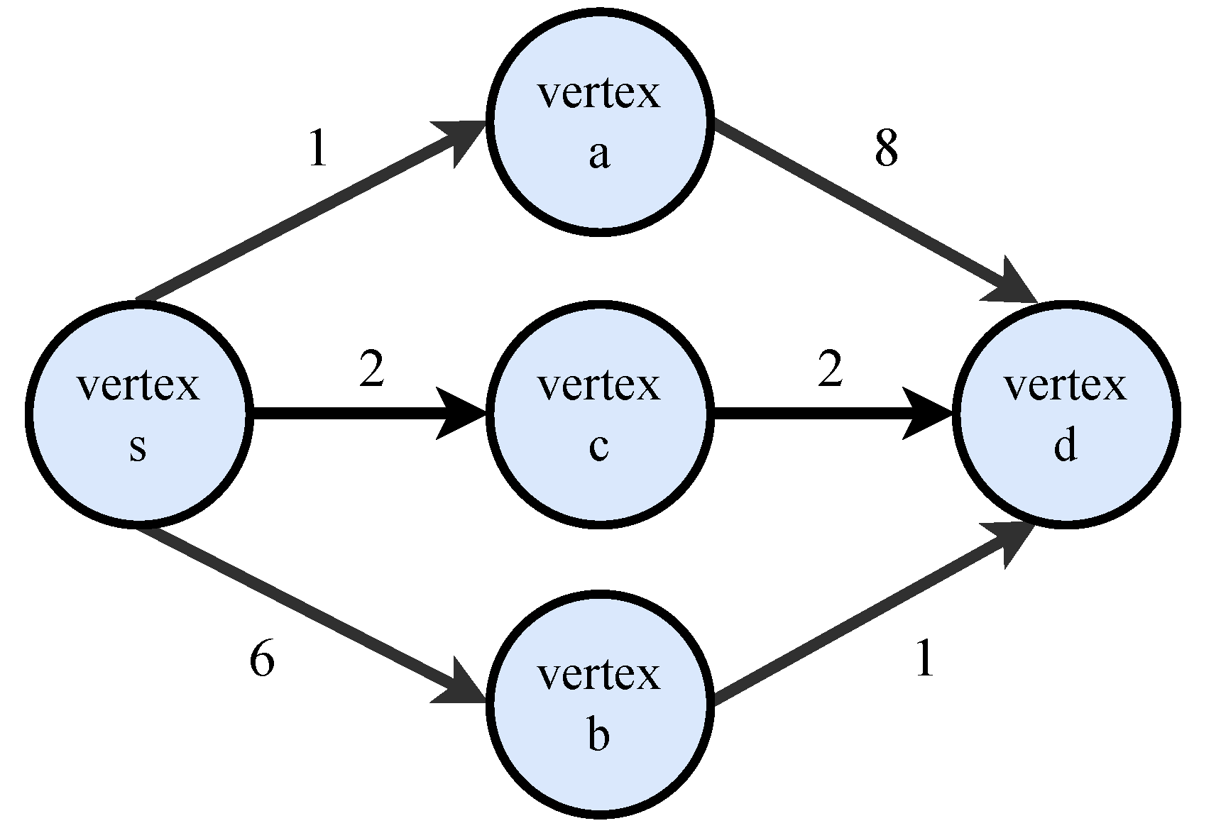
, whose cost (of the comprising edges) is minimum. Traditionally, finding the shortest path corresponds to finding the path with the shortest distance. However, to make this concept broader, here we refer to finding the route with the minimum cost (or optimal route), which better accommodates other cost definitions, such as distance, time, energy consumption, and comfort.
Figure 1 shows an example of an SP graph where the shortest path regarding the edge costs is through the vertices
.
When an SP problem is subject to vertex insertion/deletion, edge insertion/deletion, or edge cost updates over time, the problem becomes a DSP problem [
7]. This kind of problem is present in real-life applications, such as changes in route planning, as well as changes in the routing of a computer network. A naive way to approach the DSP is to run an SP algorithm from scratch whenever the graph changes. However, this approach is inefficient since the knowledge obtained in previous executions is never reused [
8]. The next subsection shows the existing classes of DSP problems in the literature [
9].
2.1. DSP Problem Classes
There are three classes of DSP problems that represent the dynamic characteristics of the problem [
10]:
Decremental dynamic shortest path: a decremental DSP problem operates only with the deletion of vertices or edges.
Incremental dynamic shortest path: unlike the decremental DSP problem, the incremental DSP operates only with the insertion of edges or vertices.
Fully dynamic shortest paths: fully DSP problems allow edges and vertices’ insertions and deletions.
Incremental and decremental dynamic shortest paths are sometimes referred to as being partially dynamic [
11]. The three DSP problem classes are still subject to the basic SP problem structure that is applied to both dynamic and static problems. The following items organize the three basic structural points of an SP problem [
12]:
Directed or undirected graphs: Directed graphs have specific directions in their edges. A directed edge from vertex s to vertex d can only be traversed from s to d, but not from d to s. In contrast, undirected graphs are those whose edges allow traversing from one vertex to another in any direction.
Weighted or unweighted graphs: Another factor that defines the structure of an SP problem is the cost to cross the edges of the graph. Weighted graphs are those with explicit costs at every edge . Unweighted graphs have no costs at their edges, so a path’s cost is defined by the number of hops (i.e., edges traversed) between the source vertex s and the destination vertex d. Unweighted graphs can be seen as a specific case of weighted graphs where all the edge costs are equal, positive, and greater than zero.
SP Problem Solution: The desired solution is also linked to the problem structure and can be split into two main categories, Single-Source Shortest Path (SSSP) and All-Pair Shortest Path (APSP). The SSSP aims to find the optimal route from a single-source vertex to all other vertices on the graph. On the other hand, APSP aims to find the optimal route for every pair of vertices on the graph.
2.2. Representative Algorithms for DSP
This section presents some of the representative algorithms for DSP problems in the literature, pointing out at the end their limitation if applied to solve an MODSP problem. The reader interested in the DSP state-of-the-art algorithms is referred to access the work of Henzinger [
13] to be redirected to those works. Moreover, it is possible to find a literature review on traffic safety in Jiang et al. [
14].
Algorithms addressed to solve the DSP problems in the literature can be exact or approximate. While the exact algorithms offer genuine responses regarding the optimal routes, the approximative algorithms propose solutions within a bound from the optimal [
15]. The choice of which type of dynamic algorithm to use can be guided by the update and query time, which measure the efficiency of dynamic algorithms.
The exact algorithms present a polynomial amortized time cost for updates on the graph
with
, where
n is the number of vertices [
16]. The disruptive work for the fully dynamic APSP on directed graphs with non-negative weights was introduced by Demetrescu and Italiano [
16]. Their work realized update operations in an amortized complexity of
and each query in
worst-case time. Moreover, the local shortest path approach and the data structure adopted by Demetrescu and Italiano served as a base motivating more researchers to exploit the exact fully dynamic APSP algorithms. This was the case for Thorup [
17], who made improvements on the Demetrescu and Italiano approach to the use of negative weights. Thorup’s work reached a
amortized update time, where
m is the number of edges, maintaining the constant query time.
Approximate algorithms, despite not guaranteeing an optimal response, present responses within a bound of the optimal (
-approximate [
18]). Those algorithms have an amortized update time cost that is almost linear [
19]. Roditty and Zwick [
20] contributed to developing approximate algorithms for incremental and decremental SSSPs, which find the shortest path with the optimal solution proximity of
in an amortized complexity of
. They also contributed with a full APSP that solves the updates with a time complexity of
, with
, a query response time in
. Brand and Nanongkai [
18] also presented a fully APSP approximate algorithm using the fast matrix technique to improve the worst-case update time to
; their work considered only directed graphs with positive weights at the edges. As a counterpart, the Brand and Nanongkai algorithm maintains only the distances and cannot report the corresponding paths.
In addition to those DSP algorithms, traffic networks are an important field in developing algorithms for the DSP problem, answering real-time traffic changes. Aiming to treat conditions such as accidents, traffic jams, and bad weather in real-time, Sever et al. [
21] proposed a framework based on dynamic programming for hybrid routing policies in transit networks. Ardakani and Sun [
22] developed an algorithm for the DSP problem considering the graph in continuous time to find the best route in real-time. Moreover, Fu and Rilett [
23] proposed a way to find the shortest paths in traffic networks subject to dynamic and stochastic changes using a heuristic algorithm based on the K-shortest path.
The main drawback of DSP algorithms is the space complexity
for storing the paths generated [
16]. This disadvantage is necessary since the stored paths are the core that allows recalculating only the affected part by the update and avoids recomputing all paths from scratch. Now, if we look forward and try to solve an MODSP problem using an off-the-shelf DSP algorithm for each objective independently, the time and space complexity end up being elevated to a prohibitive level. Moreover, combining the optimal routes per objective into a single one is not trivial [
24]. In this section, we covered the shortest path and dynamic shortest path scenarios as single-objective problems; the next section is dedicated to the MODM scenarios.
3. Multi-Objective Decision-Making
Multi-objective decision-making resembles many real-world problems. This is due to the fact that decisions are often weighted against more than one objective. When the objectives involved in decision-making are conflicting, one objective may be optimized at the expense of another one. In other words, there is a trade-off between objectives. In this scenario, all trade-offs can be optimal solutions, and this condition turns the problem into a Multi-Objective Optimization Problem (MOOP). An MOOP is composed of
d objectives
and
q decision variables
, with
denoting the decision space [
25]. Equation (
1) shows the vector of objective functions to be optimized for the MOOP resolution. The decision space
regulates the objective vector
with
, where
represents the objective space [
26].
In multi-objective optimization, there are several possible solutions considering the trade-off between objectives. Comparing possible solutions is a way to indicate which ones stand out. Using the technique of comparing solutions, it is possible to look for a solution that is as satisfactory as any other considering most of the objectives, but strictly better in at least one of the objectives of the problem [
27]. This solution is also called a non-dominated solution.
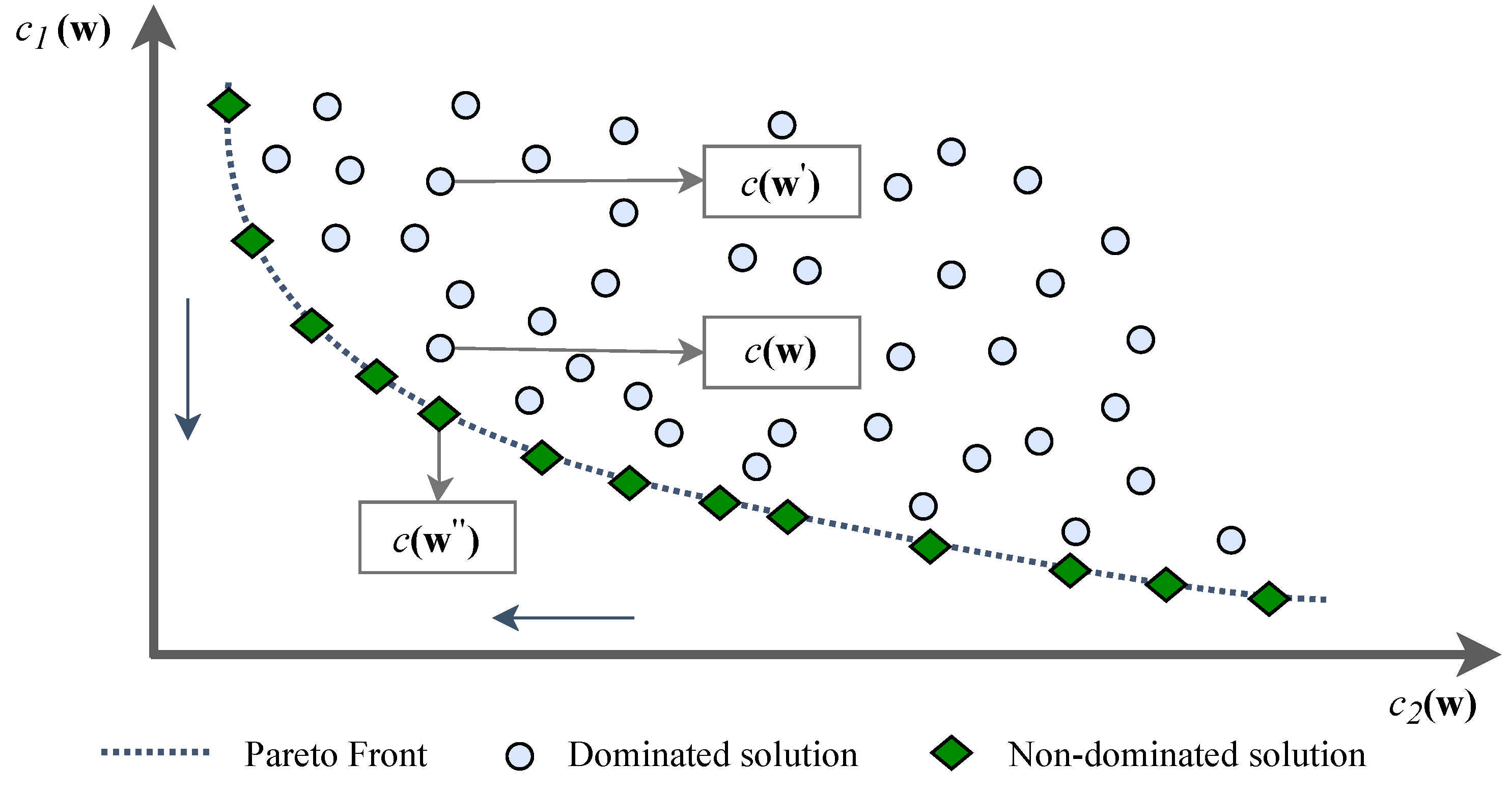
A set of non-dominated solutions in the objective space produces a boundary called the Pareto front.
Figure 2 presents a Pareto front example with non-dominated solutions (also known as optimal solutions) and dominated solutions (also known as sub-optimal solutions). Analyzing
Figure 2 from the objective
perspective, solutions
and
have the same value, i.e.,
. Now, observing from the objective
perspective, solution
is better than solution
, i.e.,
. With both objectives
and
perspectives, the solution
weakly dominates the solution
. However, the
and
solutions are not present in the Pareto front, making both sub-optimal solutions. Looking at the Pareto front, the
is an optimal solution since it dominates the solutions
and
.
An MOOP non-dominated solution enables an optimal choice for the decision-making process regarding the trade-offs between the objectives. Therefore, finding the Pareto front representing the best trade-off for the objectives solves an MOOP. However, computing an exact Pareto front can be unfeasible due to the huge number or the infinite number of non-dominated solutions [
28]. Then, a Pareto front approximation is a good approach that requires less effort and can provide a set of non-dominated solutions accurately enough to represent the exact Pareto front [
29]. With the Pareto front of the MOOP, it is possible to proceed with the decision-making process, selecting the optimal solution regarding the objectives’ importance [
24]. Then, an MODM problem is the composition of an MOOP and the decision-making process.
3.1. MODM Problem Classes
The purpose of MODM is to choose the optimal solution concerning the user’s preferences. In this way, MODM problems can be organized into three distinct classes [
27,
30]:
Known weights: In this scenario, the decision-making process already has its preferences in the form of weights that indicate the relative importance of each objective. This type of problem offers relatively small computational complexity, as it allows the direct search for the optimal Pareto solution. The scenario of known weights is usually handled with a priori methods, where a scalarization of the objectives can be determined before running the algorithm [
30,
31].
Unknown weights: In this kind of problem, the objectives’ weights are initially unknown due to the weights being subject to changes over time. In this case, a priori scalarization is unfeasible [
27]. In this context, having an approximation of the Pareto front enables a quick answer when the weights’ information is available. A solution to this problem is finding a set of solutions with at least one optimal solution for each set of weights. This set is known as the
coverage set.
Support scenario: The support scenario problem needs the user to interact with the system to indicate her/his preferences. As in the scenario with unknown weights, an approximation of the Pareto front must be found as a coverage set format. Afterwards, the user must indicate which of the optimal solutions available she/he prefers [
27,
31].
3.2. Representative Algorithms for MODM
Representative algorithms for MODM can be divided into three classes: classical mathematical-programming-based, evolutionary algorithms, and sequential decision-making algorithms with reinforcement learning. Mathematical-programming-based algorithms provide an optimal Pareto solution at each iteration. Two widely used classical methods are: the weighted sum approach [
32,
33] and the
-constraint method [
34,
35]. A major drawback of these methods is that they need expert-level knowledge about the problem to define the objective weighting factor. Otherwise, there is no guarantee that the solution will be acceptable.
Evolutionary algorithms or Multi-Objective Evolutionary Algorithms (MOEAs) define a set of candidate solutions in each new iteration using a Pareto-based classification scheme. At the end of each iteration, those algorithms find a set of candidate solutions to compose the Pareto front. A strong point of using MOEAs to find the Pareto front is the capability of finding multiple Pareto-optimal solutions in just one simulation. However, MOEAs need attention on the algorithm choice and its parameterization since, quite often, the tuning of the parameters is necessary to reach the best results with reliability, robustness, and accuracy [
36]. In addition to parameterization, there is also the issue of avoiding the local optimal solutions using fitness functions. Some of the most-important algorithms here include Non-dominated Sorting Genetic Algorithm II (NSGA-II) [
37], Strength Pareto Evolutionary Algorithm 2 (SPEA-2) [
38], the Multi-Objective Ant Colony System (MOACS) [
39], and Multi-Objective Particle Swarm Optimization (MOPSO) [
40].
Another form to address the multi-objective problems is using Sequential Decision-Making (SDM) algorithms, where the problem is modeled as a Markov Decision Process (MDP) [
24]. An MDP can be defined as a tuple
, where:
S is the state space, i.e., the set of all possible states in the environment;
A represents the action space, i.e., the set of actions the agent can take;
P specifies the transition probability function, which provides the probability of a state s subjected to action a at time step t changing to the next state at time ;
R is the reward function, specifying the reward signal obtained when performing action a in state s and transitioning to state ;
represents a discount factor, specifying the relative importance between future rewards and immediate rewards;
denotes the initial state distribution.
An SDM algorithm concerns the decision process in a given time step. This decision is dependenton the next states. Then, at each state, the SDM algorithm predicts the next best action in that state at that particular time step. SDM algorithms work with Reinforcement Learning (RL) and can produce globally optimal decision sequences, identifying the value of decisions with long-term perspectives [
26].
When the model of the environment is not available a priori, the SDM with RL approach has the advantage of learning about the dynamics of the environment during the interactions. However, this approach also has drawbacks, since the mathematical and the evolutionary methods find complete solutions, while RL needs to build solutions interactively.
The disadvantage of MODM for dealing with an MODSP problem is its inefficiency in dealing with changing environments. In particular, the insertion/deletion of a graph’s vertex or edge makes the problem non-stationary. If such a change occurs during a decision-making process, MODM will lose part of the knowledge acquired until that moment, and a systematic exploration may be necessary. With the SP, DSP, and MODM problems introduced until now, the following section presents the MOSP problem before the introduction to the MODSP for a better comprehension of the dynamic difference between both problems.
4. Multi-Objective Shortest Path
Some studies approach the MOSP as static graphs. Where most of these MOSP works are focused on bi-objective problems [
41,
42,
43,
44,
45], a small part of the works address tri-objective problems [
46,
47,
48,
49], and few works approach many objectives [
50,
51,
52]. A labeling technique extension, efficient for the single-objective purpose, is adopted by most part of these works to solve the MOSP problem [
53]. Even using a generalization of the labeling technique to solve the MOSP problem, only one path indicating the best value for all criteria is not available. Therefore, solving an MOSP problem is fundamental to search for non-dominated paths in the graph (Pareto front of the MOSP).
The labeling technique applied to the MOSP is iterative and employs the method of computing the one-to-all shortest paths, a single-source solution for the MOSP problem. We can divide the labeling technique into two: label-setting and label-correcting. Each of those labeling techniques has its own update procedure to reach the final optimal shortest paths. The key difference between both is in the estimation of the distance to the shortest path under evaluation regarding each vertex in each iteration.
For the label-setting algorithms, the vertex under evaluation searches for the least-possible label value. Then, if the optimality principle holds, each vertex is scanned at most once to reach the optimal shortest path from the source vertex to the destination vertex [
53]. This means that, in an MOSP problem, where the goal is a one-to-one optimal shortest path, the label-setting method finishes the search when it reaches the destination vertex, avoiding a more costly search in all graph vertices.
In contrast, a label-correcting algorithm may select a vertex more than once and ends after finding the shortest path from the source vertex s to all other vertices . This effect occurs since the label-correcting algorithm follows a policy to scan the graph’s vertices, for instance First In, First Out (FIFO). Moreover, the shortest path distance computed at each interaction is temporary and converges to the one-for-all optimal shortest path distances. Therefore, this scan method of the label-correcting algorithm makes the computation time to find the shortest one-to-all paths the same as that of the shortest one-to-one path.
An MOSP problem may also consider a dynamic change over time (time-dependency) regarding the objectives’ cost over the edges [
54]. This time-dependent approach to the MOSP problem considers the time window in a vertex under evaluation and the time spent to reach the neighbor vertices regarding the objectives’ cost in the current window time. In this way, a time-dependent algorithm assesses the objectives’ cost over time for each vertex under evaluation until it reaches the destination vertex [
55]. This approach is appropriate for predictable changes in graphs over time, which is applicable, for example, to determine the shortest path in a road map regarding the traffic prediction in the length of the day.
Another way to approach the MOSP problem is by using speedup techniques to search for the optimal shortest paths. This approach has a preprocessing phase that considers the objectives’ costs and a query phase to search for the optimal shortest paths. The preprocessing phase sets the Pareto-optimal paths as the most costly phase. In contrast, the query phase is remarkably fast, receiving as inputs the source vertex, destiny vertex, and weights unknown a priori to search for the shortest path with the best trade-off between the objectives’ cost and the user preferences [
56]. Geisberger et al. [
57] classified speedup methods into three classes:
Bast et al. [
60] thoroughly surveyed the speedup methods and their applications. Speedup methods are widely used in route planning on road networks without considering unpredictable updates in the graph structure [
57,
61]. For example, supposing that a new vertex needs to be inserted in the road network, the preprocessing phase needs to be rerun from scratch, not taking advantage of the previous preprocessing solution.
5. Multi-Objective Dynamic Shortest Path
Given the current panorama of the DSP and MODM research, we now turn our attention to the intersection of these two problems. This intersection results in the proposed MODSP problem as a generalization of the DSP problem with multiple objectives. The MODSP problem has multiple objectives present in the composition of the costs to traverse the graph and allows the update of the objectives’ costs at any time. Moreover, the MODSP problem involves finding the optimal path regarding the objectives between two vertices in the graph. Last but not least, the MODSP problem allows the insertion and deletion of graph edges and vertices at any time.
To better understand the MODSP problem, we start with the definition of the problem itself, followed by a taxonomy for a better view of the problem considering the MODSP and MODM problem classes and their subclasses. Finally, we present some application examples for the real world.
5.1. Problem Definition
The Multi-Objective Dynamic Shortest Path (MODSP) problem is characterized as a graph
, where
V is the set of vertices and
E is the set of edges of the graph. An edge
has its traversing cost
addressed by
d objectives
. The trade-off between the objectives is regulated by the decision variable vector
composed of
q decision variables
, resulting in Equation (
1). Then, with the cost vector
(from an edge or a path) and the decision variable vector
, it is possible to designate a linear scalarization function and compute the inner product from both vectors
.
We can express the vertex sequence of a path
from vertex
x to vertex
y by
,
,
, and
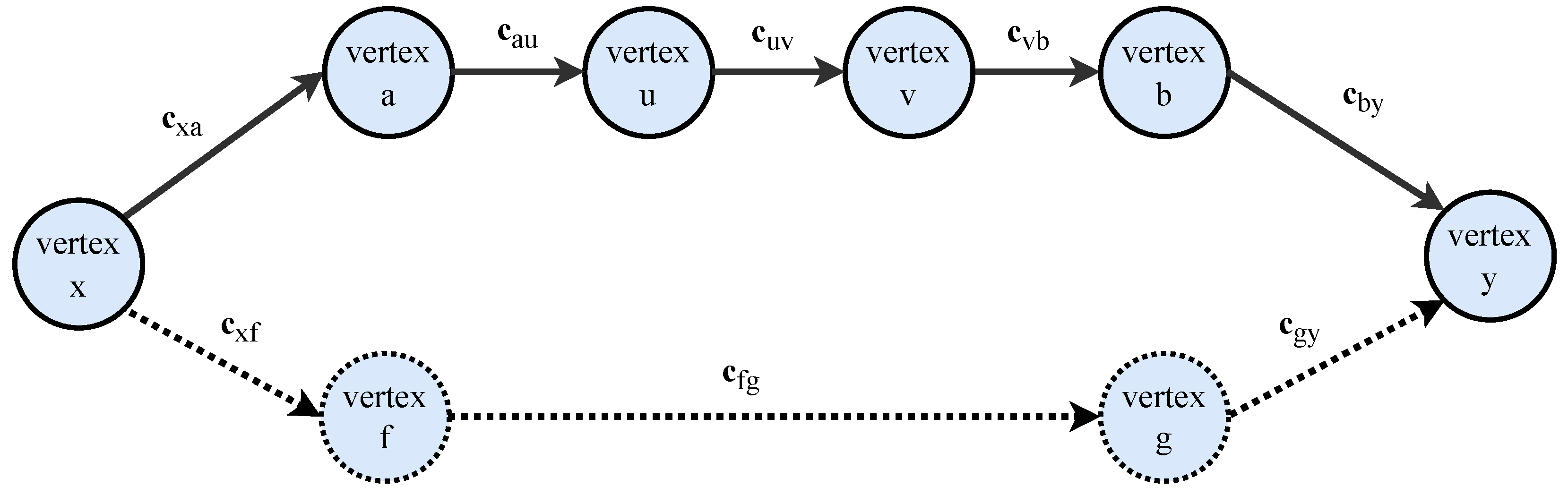
for each
. Observing the edge
from
Figure 3, its multi-objective cost to traverse the vertex
u to
v is expressed by
. Moreover, we can denote the multi-objective cost of a path
by
and its linear scalarization regarding the decision variables by
.
A special case in modeling the MODSP problem is a path from a vertex
x to itself
, where all the objectives’ costs are equal to zero. Observing
Figure 3, a concatenation between the paths
and
can be written as
. Finally, we denote the path
as the left subpath
to compose the path
in the same way and the path
as the right subpath
to compose the path
.
We can observe two moments for choosing a path
in
Figure 3. In the first moment, assume that vertices
f and
g do not exist in the graph. In this case, the possible path is through vertices
. Choosing this unique available path results in a cost denoted by
, which can be expressed as
. In the second moment, assuming new vertices
f and
g are inserted in the graph, it is necessary to consider the newly available path through the new vertices verifying if the solution is non-dominated. In this case, the new path has a cost denoted by
or
.
As we mentioned before, an MODSP problem is subjected to an unforeseen sequence of vertex updates. To maintain these properties, the MODSP problem is subject to the following operations:
update : This procedure allows dynamic changes in the graph structure, updating, inserting, or removing the vertex v and the cost vector of all edges connected to the vertex v. Furthermore, this procedure updates only the paths that cross the vertex v, taking advantage of the previous solution not affected by the update;
pf_sp : a procedure that returns the approximate Pareto front of optimal shortest paths from vertex x to vertex y, if any;
cost_sp : a query procedure that receives as the input the source vertex x, the destination vertex y, and the decision variables ‘vector , returning optimal cost vector from the optimal shortest path, if any;
optimal_sp : This query procedure uses the inputs’ source vertex x, destination vertex y, and the decision variables’ vector to return the optimal shortest path considering the best trade-off between the decision variables’ vector and the cost vector , if any.
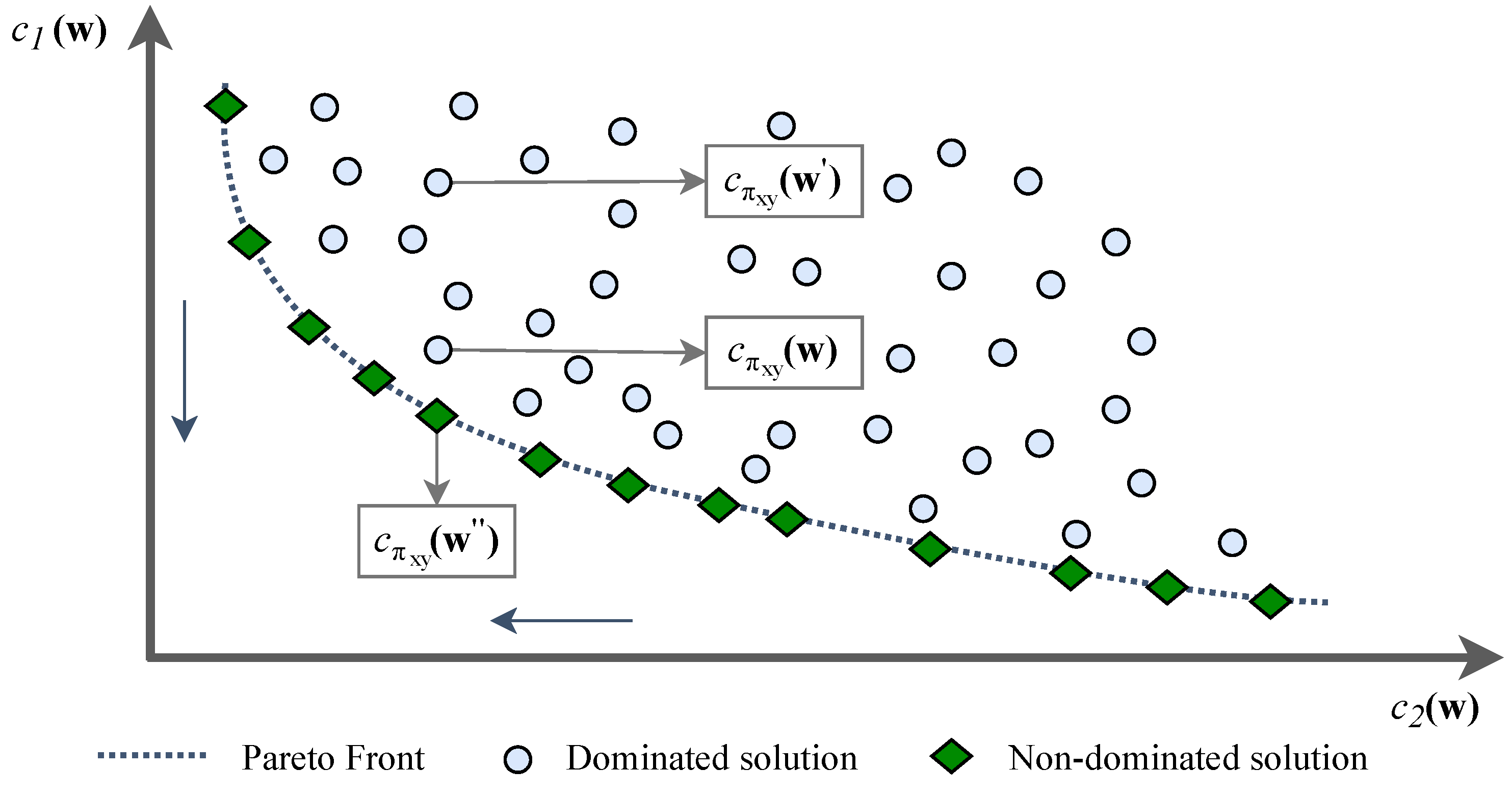
Bringing
Figure 2 to the MODSP context, we can have several possible solutions considering the trade-off between the objectives for only one desired path
.
Figure 4 shows the same example of the Pareto front of
Figure 2, in which we changed the solutions’ nomenclature to possible paths to facilitate the understanding of the proposed problem. Next, we rewrite the description given in
Section 3 for the context of the MODSP problem. In
Figure 4, when comparing the solutions
and
, considering only the objective
, we have the solution
as dominant,
. However, when considering the goal
, both solutions have the same value,
. Thus, the solution
weakly dominates the solution
, and both solutions are sub-optimal due to being out of the Pareto front. Finally, the
solution is an example of a non-dominated solution present on the Pareto front for a specific trade-off defined for
.
The set of non-dominated solutions of a path contains the best trade-offs for the multiple objectives. Thus, the MODSP solution regards maintaining the sets of non-dominated shortest paths up to date after each vertex update operation, taking advantage of previously computed solutions. In this way, the decision-making process can proceed with the query procedures.
5.2. MODSP Taxonomy
In order to make the MODSP problem more visible as a class of problems,
Figure 5 shows a taxonomy, with our view of the problem classes that deal with the shortest path problems. Starting the taxonomy analysis by segregating the five classes involved in the Venn diagram, we can observe that the three problem classes, the MODSP, DSP, and MODM, are well delimited in the taxonomy. We represent the MOSP problem class in the taxonomy as the intersection between the MODM and MODSP problem classes. Our claim that the MOSP is the intersection between MODM and the MODSP implies that the MOSP definition can neither represent dynamic structural changes in the graph over time nor represent graph-less problems with multiple objectives. In the same way, the SP problem class is presented in the taxonomy as an intersection area between the DSP and MOSP class of problems. As the SP problem is a subclass of the DSP and MOSP class of problems, the SP problem class does not have the multiple objectives from the MOSP problem class and does not have the dynamic graph structural changes over time from the DSP problem class.
By analyzing the taxonomy, it is possible to observe that the SP and MOSP problems are subclasses of the MODM since they can be solved using multi-objective reinforcement learning methods [
30]. Furthermore, the MODM problem class can solve other non-graph-related problems, as represented in
Figure 5, by the area that does not intersect with the MODSP problem class. However, the MODM problem class cannot solve graph problems with dynamic changes like the MODSP and DSP problems due to the possibility of inserting or removing vertices and edges at any time [
1,
12]. Taking the analysis to the bias of the MODSP problem class, it is possible to observe that the MODSP methods can solve all problems related to graphs since the DSP, MOSP, and SP problem classes are subclasses of the MODSP problem class. Our taxonomy of the MODSP problem class sheds light on a challenging problem in emerging areas, such as the evolution of telecommunications networks and autonomous vehicles. These emerging areas make MODSP more evident in real-world situations, requiring attention to be resolved appropriately and avoiding delayed and inaccurate responses.
To the best of our knowledge, until our previous work [
3], no others in the literature dealt completely with MODSP. The closest works considered only MOSP approaches [
41,
42,
43,
46,
47,
48,
50,
51]. The MODSP distinguishes itself from the MOSP since it requires a solution or an update after an online structural change on the graph. Due to the absence of the dynamic and unpredictable update component in the problem formulation, the MOSP needs to recalculate the shortest paths from scratch when the insertion or deletion of a route in the graph occurs. However, recalculating optimal routes from scratch is inefficient since changes in the graph may occur at exclusive points. Thus, in the MODSP algorithmic perspective, the graph changes are evaluated, and the update is executed only on the affected paths. Concerning the problem’s complexity, the MOSP is NP-hard [
68,
69], which also makes the MODSP at least NP-hard.
6. Applications
The list of potential applications of the MODSP is increasing steadily, especially with the advent of smart cities, autonomous vehicles, smart devices, the Internet of Things, etc. Furthermore, access to mobile networks allows smart devices to benefit from the MODSP when choosing and updating a displacement. At the same time, the MODSP applications can still vary between leisure and strategic decisions. Therefore, this section presents a few selected strategic scenarios for the application of the MODSP.
6.1. Intelligent Transportation Systems
Traffic networks comprise a problem addressed to the transportation systems that involves numerous variables to be satisfied, e.g., time travel, distance, safety (drainage problems, weather, and lack of illumination), and travel costs [
70,
71,
72]. All those variables can be updated dynamically with a real-time system, as indicated in the work of Sohrabi and Lord [
73]. Therefore, we see the traffic networks as an MODSP problem since the problem can receive real-time updates regarding the objectives cost and changes in the graph topology due to incidents that can close or open roads at any time. Moreover, the optimal shortest path result will be subjected to user preferences where a user selects a fast travel time rather than driving a short distance.
Works addressed to transportation systems consider the traffic networks dynamic when the weight changes over time or the objectives’ cost follows a pattern. However, as Sohrabi and Lord [
73] listed in their work, the desired requirements for a safe-route-finding system regard the capability to update the graph information in real-time with the support of sensors and dealing with trade-offs over the travel time. Then, following this future of the traffic network problem, the MODSP problem fits as a better model for developing new solutions.
Moreover, another current traffic network problem that calls our attention is the navigation system used by self-driving cars. In such a problem, vehicles are also subject to dynamic environmental changes. Therefore, they need to accommodate multiple objectives regarding the optimal route choice, such as travel time, comfort, energy consumption, obstacles, distance to be covered, and threats to passengers and pedestrians [
60,
73,
74,
75].
6.2. Military Path-Finding
Military path-finding is a problem for the chain of command and control in carrying out military missions. Military missions are considered highly dynamic and uncertain when involving human lives. Military path-finding is dynamic due to the nature of the battlefield, where the terrain and enemies can change at any time. Moreover, the missions are uncertain factors due to the multiple objectives present in the mission, such as the visibility of the terrain, distance, difficulty in accessing the route, execution time, cost operations, and exposure to threats.
Some works address the problem with a focus only on the multi-objective issue, leaving the displacement route in enemy territory undefined [
76]. More comprehensive works deal with displacement and the multiple objectives involved in the mission [
77,
78]. However, these works do not consider route insertion or deletion when troops traverse the path. Considering existing results for the military path-finding problem, a complete MODSP approach remains an open problem.
6.3. Routing Protocols
Internet routing has a dynamic nature because a link may change its status to up or down during the transmission of the packets. Besides that, routing protocols are MODM problems as well [
79,
80,
81,
82], where the objectives may be listed as:
Maximizing bandwidth, thus allowing for rapid transfer of data between nodes;
Minimizing latency, to keep buffering low during distributed real-time applications;
Maximizing redundancy, then providing multiple data paths so that connectivity is preserved if some nodes go offline.
Routing protocol challenges are present in streaming platforms with a high bandwidth, as well as real-time applications such as video calls requesting low latency. Given these requirements, routing can be modeled as an MODSP problem, where the system can dynamically redirect traffic flow to achieve better results.
6.4. Unmanned Aerial Vehicles
Unmanned Aerial Vehicles (UAVs)/drones are increasingly used in many activities, reducing life-threatening conditions or in environments with restrictive access. For example, UAVs can deliver packages, film live sports, and search for people for diverse purposes [
83,
84,
85]. For these applications, UAVs should consider other obstacles along the path, such as other drones or even trees and traffic signs; moreover, they should also reduce energy consumption to cover larger areas [
86]. To this end, the UAVs fit the definition of the MODSP to accomplish the dynamic changes in the environment and multiple objectives’ cost.
7. Challenges and Open Questions
Recent years have seen a relevant breakthrough regarding multi-objective and shortest-path algorithms due to complex real-world problems. However, as presented in
Section 5, this work opens a new research niche for the shortest-path problems unifying the dynamic and multi-objective approaches resulting in the MODSP problem. Since the MODSP is a new problem proposal, a number of significant and pressing challenges for the MODSP research need to be intensified. In this context, the remainder of this section will present an overview of these challenges.
7.1. Lack of Multi-Objective Dynamic Shortest Path Datasets
The datasets are essential to perform tests and develop algorithms capable of solving the MODSP problem. The proposal to adopt the MOSP dataset made by da Silva et al. [
3], using the initial dataset to build the graph update datasets, is valid for testing. In the approach by da Silva et al., the creation of the graph update dataset starts with choosing a random vertex and all edges that connect with the selected vertex generating the new dataset for update purposes. However, this type of approach may not be sufficient a priori, as the datasets for updating may be presented in a more complex way and correlated with real-life problems. The datasets for updating should also cover the insertion of new vertices not present in the graph’s initial form, and the removal of vertices from the graph enable this. This challenge of finding or building datasets can slow down and even hinder researchers’ progress on the MODSP problem. Then, actions towards this challenge are related to the disposal of MODSP problems, data, benchmarks, and baseline implementations available on open platforms.
7.2. Lack of Algorithmic Benchmarks
Given the novelty of the MODSP problem, there is a lack of possible solutions, bringing to light the need to engage more researchers in the area. This challenge is directly related to helping other researchers interested in the MODSP. One possibility is the creation of a repository of algorithms following a unified standard in order to facilitate the benchmark of new methods that may be developed in the future. In this way, newly proposed algorithms to solve the MODSP problem will emerge and allow an adequate benchmark between them. Such engagement of more researchers could bring benefits to our society in solving the MODSP problem and taking it to applications in real-world problems.
7.3. Algorithmic Analysis for a Better Evaluation of the MODSP Solutions
Even with the lack of algorithms to solve the MODSP problem, the question of the true advantage of using such solutions remains open. The challenge for this type of questioning is finding an answer in the analysis from the theoretical point of view through asymptotic analysis. One piece of evidence of needing a theoretical analysis of existing algorithms was presented in the work by da Silva et al., where it was clear that the cost of generating paths at the first moment is very high, surpassing an MOSP algorithm. However, the cost of updating in a second moment has a significant advantage over other algorithms. In this way, it is evident that an asymptotic analysis of the MODSP algorithms is necessary to evaluate in what circumstances or situations there are advantages in using these algorithms about the others of the DSP or MOSP considering an MODSP problem for the resolution.
8. Concluding Remarks
This article generalized the dynamic shortest path problem, which determines routes in graphs subject to the insertion, deletion, and update of edges and vertices, where the cost of crossing the edges comprises multiple objectives subjected to decision variables unknown at first. We refer to this problem as the Multi-Objective Dynamic Shortest Path (MODSP) problem since it lies at the intersection of two widely explored problems, namely the Dynamic Shortest Path (DSP) and Multi-Objective Decision Making (MODM). To this end, we described the DSP and MODM problem classes focused on the works that inspired the proposal of the MODSP problem. Moreover, we also described the Multi-Objective Shortest Path (MOSP) problem and the time-dependent MOSP problem evidencing the differences with the MODSP problem.
Furthermore, this article described the theoretical formulation of the MODSP problem by presenting a taxonomy in Venn diagram format. The taxonomy introduced the MODSP problem class and its relationship with the MODM, DSP, MOSP, and SP problem classes. Considering that the MODSP problem covers many complex situations in the real world, some applications were suggested so that the problems bring motivation to be treated more thoroughly in future works. In addition, we provided our current view of the challenges and open questions for the MODSP problem.
More than formalizing or delimiting the MODSP problem, this work aimed to draw researchers’ attention to this relevant class of problems. Considering current technologies, such as sensors and devices connected in the cloud, we reach real-time conditions reflecting route systems much more dynamically than years ago. Therefore, we believe the MODSP problem cannot be neglected currently due to its great practical importance, as many applications depend on this approach to find satisfactory solutions.
Author Contributions
Conceptualization, J.M.d.S.; investigation, J.M.d.S.; methodology, J.M.d.S.; supervision, G.d.O.R. and J.L.V.B.; writing—original draft, J.M.d.S.; writing—review and editing, G.d.O.R. and J.L.V.B. All authors have read and agreed to the published version of the manuscript.
Funding
This research was partially supported by Coordenação de Aperfeiçoamento de Pessoal de Nível Superior, Brasil (CAPES), Finance Code 001, Conselho Nacional de Desenvolvimento Científico e Tecnológico (CNPq) (grant 306395/2017-7), Fundação de Amparo à Pesquisa do Estado do Rio Grande do Sul (FAPERGS) (Grants 17/2551-0001197-0 and 19/2551-0001277-2), and Fundação de Amparo à Pesquisa do Estado de São Paulo (FAPESP) (Grant 2020/05165-1).
Institutional Review Board Statement
Not applicable.
Informed Consent Statement
Not applicable.
Data Availability Statement
Not applicable.
Acknowledgments
This research was partially supported by Coordenação de Aperfeiçoamento de Pessoal de Nível Superior, Brasil (CAPES), Finance Code 001, Conselho Nacional de Desenvolvimento Científico e Tecnológico (CNPq) (grant 306395/2017-7), Fundação de Amparo à Pesquisa do Estado do Rio Grande do Sul (FAPERGS) (Grants 17/2551-0001197-0 and 19/2551-0001277-2), and Fundação de Amparo à Pesquisa do Estado de São Paulo (FAPESP) (Grant 2020/05165-1).
Conflicts of Interest
The authors declare no conflict of interest.
References
- Ferone, D.; Festa, P.; Napoletano, A.; Pastore, T. Shortest paths on dynamic graphs: A survey. Pesqui. Oper. 2017, 37, 487–508. [Google Scholar] [CrossRef] [Green Version]
- Tanabe, R.; Ishibuchi, H. An Easy-to-Use Real-World Multi-Objective Optimization Problem Suite. Appl. Soft Comput. 2020, 89, 106078. [Google Scholar] [CrossRef]
- Da Silva, J.M.; de O. Ramos, G.; Barbosa, J.L.V. The multi-objective dynamic shortest path problem. In Proceedings of the 2022 IEEE Congress on Evolutionary Computation (CEC), Padua, Italy, 18–23 July 2022; pp. 1–8. [Google Scholar] [CrossRef]
- Demetrescu, C.; Italiano, G.F. Experimental Analysis of Dynamic All Pairs Shortest Path Algorithms. ACM Trans. Algorithms 2006, 2, 578–601. [Google Scholar] [CrossRef] [Green Version]
- Fortz, B.; Thorup, M. Internet traffic engineering by optimizing OSPF weights. In Proceedings of the Proceedings IEEE INFOCOM 2000. Conference on Computer Communications. Nineteenth Annual Joint Conference of the IEEE Computer and Communications Societies (Cat. No.00CH37064), Tel Aviv, Israel, 26–30 March 2000; Volume 2, pp. 519–528. [Google Scholar] [CrossRef]
- Narvaez, P.; Siu, K.Y.; Tzeng, H.Y. New dynamic algorithms for shortest path tree computation. IEEE/ACM Trans. Netw. 2000, 8, 734–746. [Google Scholar] [CrossRef]
- Ramalingam, G.; Reps, T. On the computational complexity of dynamic graph problems. Theor. Comput. Sci. 1996, 158, 233–277. [Google Scholar] [CrossRef] [Green Version]
- Baswana, S.; Khurana, S.; Sarkar, S. Fully Dynamic Randomized Algorithms for Graph Spanners. ACM Trans. Algorithms 2012, 8. [Google Scholar] [CrossRef] [Green Version]
- Sunita; Garg, D. Dynamizing Dijkstra: A solution to dynamic shortest path problem through retroactive priority queue. J. King Saud Univ.—Comput. Inf. Sci. 2021, 33, 364–373. [Google Scholar] [CrossRef]
- Roditty, L.; Zwick, U. On Dynamic Shortest Paths Problems. Algorithmica 2011, 61, 389–401. [Google Scholar] [CrossRef] [Green Version]
- Demetrescu, C.; Italiano, G.F. Dynamic shortest paths and transitive closure: Algorithmic techniques and data structures. J. Discret. Algorithms 2006, 4, 353–383. [Google Scholar] [CrossRef]
- Madkour, A.; Aref, W.G.; Rehman, F.U.; Rahman, M.A.; Basalamah, S. A survey of shortest-path algorithms. arXiv 2017, arXiv:1705.02044. [Google Scholar] [CrossRef]
- Henzinger, M. The State of the Art in Dynamic Graph Algorithms. In SOFSEM 2018: Theory and Practice of Computer Science, Proceedings of the 44th International Conference on Current Trends in Theory and Practice of Computer Science, Krems, Austria, 29 January–2 February 2018; Tjoa, A.M., Bellatreche, L., Biffl, S., van Leeuwen, J., Wiedermann, J., Eds.; Springer International Publishing: Cham, Switzerland, 2018; pp. 40–44. [Google Scholar] [CrossRef]
- Jiang, S.; Zhang, Y.; Liu, R.; Jafari, M.; Kharbeche, M. Data-Driven Optimization for Dynamic Shortest Path Problem Considering Traffic Safety. IEEE Trans. Intell. Transp. Syst. 2022, 23, 18237–18252. [Google Scholar] [CrossRef]
- Zwick, U. Exact and Approximate Distances in Graphs—A Survey. In Algorithms—ESA 2001, Proceedings of the 9th Annual European Symposium, Aarhus, Denmark, 28–31 August 2001; auf der Heide, F.M., Ed.; Springer: Berlin/Heidelberg, Germany, 2001; pp. 33–48. [Google Scholar] [CrossRef]
- Demetrescu, C.; Italiano, G.F. A New Approach to Dynamic All Pairs Shortest Paths. J. ACM 2004, 51, 968–992. [Google Scholar] [CrossRef] [Green Version]
- Thorup, M. Fully-Dynamic All-Pairs Shortest Paths: Faster and Allowing Negative Cycles. In Algorithm Theory—SWAT 2004, Proceedings of the 9th Scandinavian Workshop on Algorithm Theory, Humlebaek, Denmark, 8–10 July 2004; Hagerup, T., Katajainen, J., Eds.; Springer: Berlin/Heidelberg, Germany, 2004; pp. 384–396. [Google Scholar] [CrossRef]
- Van den Brand, J.; Nanongkai, D. Dynamic Approximate Shortest Paths and Beyond: Subquadratic and Worst-Case Update Time. In Proceedings of the 2019 IEEE 60th Annual Symposium on Foundations of Computer Science (FOCS), Baltimore, MD, USA, 9–12 November 2019; pp. 436–455. [Google Scholar] [CrossRef] [Green Version]
- Bernstein, A. Fully dynamic (2 + ε) approximate all-pairs shortest paths with fast query and close to linear update time. In Proceedings of the 2009 50th Annual IEEE Symposium on Foundations of Computer Science, Atlanta, GA, USA, 25–27 October 2009; pp. 693–702. [Google Scholar] [CrossRef]
- Roditty, L.; Zwick, U. Dynamic Approximate All-Pairs Shortest Paths in Undirected Graphs. SIAM J. Comput. 2012, 41, 670–683. [Google Scholar] [CrossRef]
- Sever, D.; Dellaert, N.; van Woensel, T.; de Kok, T. Dynamic shortest path problems: Hybrid routing policies considering network disruptions. Comput. Oper. Res. 2013, 40, 2852–2863. [Google Scholar] [CrossRef]
- Ardakani, M.K.; Sun, L. Decremental algorithm for adaptive routing incorporating traveler information. Comput. Oper. Res. 2012, 39, 3012–3020. [Google Scholar] [CrossRef]
- Fu, L.; Rilett, L. Expected shortest paths in dynamic and stochastic traffic networks. Transp. Res. Part B Methodol. 1998, 32, 499–516. [Google Scholar] [CrossRef]
- Roijers, D.M.; Vamplew, P.; Whiteson, S.; Dazeley, R. A Survey of Multi-Objective Sequential Decision-Making. J. Artif. Int. Res. 2013, 48, 67–113. [Google Scholar] [CrossRef] [Green Version]
- Deb, K. Multi-Objective Optimization. In Search Methodologies: Introductory Tutorials in Optimization and Decision Support Techniques; Springer: Boston, MA, USA, 2005; pp. 273–316. [Google Scholar] [CrossRef]
- Wang, W. Multi-Objective Sequential Decision Making. Ph.D. Thesis, Université Paris Sud-Paris—XI, Bures-sur-Yvette, France, 2014. Available online: https://theses.hal.science/tel-01057079 (accessed on 15 March 2023).
- Roijers, D.M.; Whiteson, S. Multi-Objective Decision Making; Number 1; Springer International Publishing: New York, NY, USA, 2017; pp. 1–129. [Google Scholar] [CrossRef]
- Mandow, L.; Perez-de-la Cruz, J.L.; Pozas, N. Multi-objective dynamic programming with limited precision. J. Glob. Optim. 2022, 82, 595–614. [Google Scholar] [CrossRef]
- Ruzika, S.; Wiecek, M.M. Approximation Methods in Multiobjective Programming. J. Optim. Theory Appl. 2005, 126, 473–501. [Google Scholar] [CrossRef]
- Hayes, C.F.; Rădulescu, R.; Bargiacchi, E.; Källström, J.; Macfarlane, M.; Reymond, M.; Verstraeten, T.; Zintgraf, L.M.; Dazeley, R.; Heintz, F.; et al. A practical guide to multi-objective reinforcement learning and planning. Auton. Agents Multi-Agent Syst. 2022, 36, 1–59. [Google Scholar] [CrossRef]
- Rădulescu, R.; Mannion, P.; Roijers, D.M.; Nowé, A. Multi-Objective Multi-Agent Decision Making: A Utility-Based Analysis and Survey. Auton. Agents Multi-Agent Syst. 2019, 34, 10. [Google Scholar] [CrossRef] [Green Version]
- Miettinen, K. Nonlinear Multiobjective Optimization; Springer: Boston, MA, USA, 1998; Volume 12, pp. 1–319. [Google Scholar] [CrossRef]
- Ehrgott, M. Multicriteria Optimization; Springer: Berlin/Heidelberg, Germany, 2005; pp. 1–336. [Google Scholar] [CrossRef] [Green Version]
- Haimes, Y. On a Bicriterion Formulation of the Problems of Integrated System Identification and System Optimization. IEEE Trans. Syst. Man Cybern. 1971, 3, 296–297. [Google Scholar] [CrossRef]
- Mavrotas, G. Effective implementation of the ε-constraint method in Multi-Objective Mathematical Programming problems. Appl. Math. Comput. 2009, 213, 455–465. [Google Scholar] [CrossRef]
- Wang, Q.; Wang, L.; Huang, W.; Wang, Z.; Liu, S.; Savić, D.A. Parameterization of NSGA-II for the Optimal Design of Water Distribution Systems. Water 2019, 11, 971. [Google Scholar] [CrossRef] [Green Version]
- Deb, K.; Pratap, A.; Agarwal, S.; Meyarivan, T. A fast and elitist multiobjective genetic algorithm: NSGA-II. IEEE Trans. Evol. Comput. 2002, 6, 182–197. [Google Scholar] [CrossRef] [Green Version]
- Zitzler, E.; Laumanns, M.; Thiele, L. SPEA2: Improving the strength pareto evolutionary algorithm. TIK Rep. 2001, 103, 1–22. [Google Scholar] [CrossRef]
- Gao, Y.; Guan, H.; Qi, Z.; Hou, Y.; Liu, L. A multi-objective ant colony system algorithm for virtual machine placement in cloud computing. J. Comput. Syst. Sci. 2013, 79, 1230–1242. [Google Scholar] [CrossRef]
- Coello Coello, C.; Lechuga, M. MOPSO: A proposal for multiple objective particle swarm optimization. In Proceedings of the 2002 Congress on Evolutionary Computation. CEC’02 (Cat. No.02TH8600), Honolulu, HI, USA, 12–17 May 2002; Volume 2, pp. 1051–1056. [Google Scholar] [CrossRef]
- He, F.; Qi, H.; Fan, Q. An evolutionary algorithm for the multi-objective shortest path problem. In Proceedings of the International Conference on Intelligent Systems and Knowledge Engineering, Chengdu, China, 15–16 October 2007; Atlantis Press: Paris, France, 2007. [Google Scholar] [CrossRef] [Green Version]
- Sedeño-Noda, A.; Raith, A. A Dijkstra-like method computing all extreme supported non-dominated solutions of the biobjective shortest path problem. Comput. Oper. Res. 2015, 57, 83–94. [Google Scholar] [CrossRef]
- Duque, D.; Lozano, L.; Medaglia, A.L. An exact method for the biobjective shortest path problem for large-scale road networks. Eur. J. Oper. Res. 2015, 242, 788–797. [Google Scholar] [CrossRef]
- Guo, Q.; Wang, N.; Su, B.; Zhang, M. Bi-Objective Vehicle Routing for Muck Transportation in Urban Road Networks. IEEE Access 2020, 8, 114219–114227. [Google Scholar] [CrossRef]
- Prakash, V.P.; Patvardhan, C.; Srivastav, A. A novel Hybrid Multi-objective Evolutionary Algorithm for the bi-Objective Minimum Diameter-Cost Spanning Tree (bi-MDCST) problem. Eng. Appl. Artif. Intell. 2020, 87, 103237. [Google Scholar] [CrossRef]
- Jun, H.; Qingbao, Z. Multi-objective Mobile Robot Path Planning Based on Improved Genetic Algorithm. In Proceedings of the 2010 International Conference on Intelligent Computation Technology and Automation, Changsha, China, 11–12 May 2010; Volume 2, pp. 752–756. [Google Scholar] [CrossRef]
- Ahmed, F.; Deb, K. Multi-objective optimal path planning using elitist non-dominated sorting genetic algorithms. Soft Comput. 2013, 17, 1283–1299. [Google Scholar] [CrossRef]
- Hidalgo-Paniagua, A.; Vega-Rodríguez, M.A.; Ferruz, J.; Pavón, N. Solving the Multi-Objective Path Planning Problem in Mobile Robotics with a Firefly-Based Approach. Soft Comput. 2017, 21, 949–964. [Google Scholar] [CrossRef]
- Weise, J.; Mai, S.; Zille, H.; Mostaghim, S. On the Scalable Multi-Objective Multi-Agent Pathfinding Problem. In Proceedings of the 2020 IEEE Congress on Evolutionary Computation (CEC), Glasgow, UK, 19–24 July 2020; pp. 1–8. [Google Scholar] [CrossRef]
- Pulido, F.J.; Mandow, L.; de-la Cruz, J.L.P. Dimensionality reduction in multiobjective shortest path search. Comput. Oper. Res. 2015, 64, 60–70. [Google Scholar] [CrossRef]
- Tozer, B.; Mazzuchi, T.; Sarkani, S. Many-objective stochastic path finding using reinforcement learning. Expert Syst. Appl. 2017, 72, 371–382. [Google Scholar] [CrossRef]
- Ren, Z.; Rathinam, S.; Choset, H. Subdimensional Expansion for Multi-Objective Multi-Agent Path Finding. IEEE Robot. Autom. Lett. 2021, 6, 7153–7160. [Google Scholar] [CrossRef]
- Paixão, J.M.; Santos, J.L. Labeling Methods for the General Case of the Multi-objective Shortest Path Problem—A Computational Study. In Computational Intelligence and Decision Making; Madureira, A., Reis, C., Marques, V., Eds.; Springer: Dordrecht, The Netherlands, 2013; pp. 489–502. [Google Scholar] [CrossRef]
- Ding, B.; Yu, J.X.; Qin, L. Finding Time-Dependent Shortest Paths over Large Graphs. In Proceedings of the 11th International Conference on Extending Database Technology: Advances in Database Technology, EDBT’08, Nantes, France, 25–29 March 2008; Association for Computing Machinery: New York, NY, USA, 2008; pp. 205–216. [Google Scholar] [CrossRef]
- Wang, Y.; Yuan, Y.; Ma, Y.; Wang, G. Time-Dependent Graphs: Definitions, Applications, and Algorithms. Data Sci. Eng. 2019, 4, 352–366. [Google Scholar] [CrossRef] [Green Version]
- Funke, S.; Storandt, S. Polynomial-time Construction of Contraction Hierarchies for Multi-criteria Objectives. In Proceedings of the 2013 Proceedings of the Meeting on Algorithm Engineering and Experiments (ALENEX), SIAM, New Orleans, LA, USA, 7 January 2013; pp. 41–54. [CrossRef] [Green Version]
- Geisberger, R.; Kobitzsch, M.; Sanders, P. Route Planning with Flexible Objective Functions. In Proceedings of the 2010 Proceedings of the Workshop on Algorithm Engineering and Experiments (ALENEX), SIAM, Austin, TX, USA, 16 January 2010; pp. 124–137. [CrossRef] [Green Version]
- Geisberger, R.; Sanders, P.; Schultes, D.; Delling, D. Contraction Hierarchies: Faster and Simpler Hierarchical Routing in Road Networks. In Experimental Algorithms, Proceedings of the 7th International Workshop, WEA 2008 Provincetown, MA, USA, 30 May–1 June 2008; McGeoch, C.C., Ed.; Springer: Berlin/Heidelberg, Germany, 2008; pp. 319–333. [Google Scholar] [CrossRef]
- Goldberg, A.V.; Harrelson, C. Computing the Shortest Path: A Search Meets Graph Theory. In Proceedings of the Sixteenth Annual ACM-SIAM Symposium on Discrete Algorithms, SODA ’05, Vancouver, BC, Canada, 23–25 January 2005; Society for Industrial and Applied Mathematics: Philadelphia, PA, USA, 2005; pp. 156–165. [Google Scholar] [CrossRef]
- Bast, H.; Delling, D.; Goldberg, A.; Müller-Hannemann, M.; Pajor, T.; Sanders, P.; Wagner, D.; Werneck, R.F. Route Planning in Transportation Networks. In Algorithm Engineering: Selected Results and Surveys; Springer International Publishing: Cham, Switzerland, 2016; pp. 19–80. [Google Scholar] [CrossRef] [Green Version]
- Rajan, P.; Ravishankar, C.V. Stochastic Route Planning for Electric Vehicles. In Proceedings of the 20th International Symposium on Experimental Algorithms (SEA 2022), Heidelberg, Germany, 25–27 July 2022; Schulz, C., Uçar, B., Eds.; Leibniz International Proceedings in Informatics (LIPIcs). Schloss Dagstuhl—Leibniz-Zentrum für Informatik: Dagstuhl, Germany, 2022; Volume 233, pp. 15:1–15:17. [Google Scholar] [CrossRef]
- Zajac, S.; Huber, S. Objectives and methods in multi-objective routing problems: A survey and classification scheme. Eur. J. Oper. Res. 2021, 290, 1–25. [Google Scholar] [CrossRef]
- Mandow, L.; De La Cruz, J.L.P. Multiobjective A* Search with Consistent Heuristics. J. ACM 2008, 57, 1–25. [Google Scholar] [CrossRef]
- Skriver, A.; Andersen, K. A label correcting approach for solving bicriterion shortest-path problems. Comput. Oper. Res. 2000, 27, 507–524. [Google Scholar] [CrossRef]
- Tung Tung, C.; Lin Chew, K. A multicriteria Pareto-optimal path algorithm. Eur. J. Oper. Res. 1992, 62, 203–209. [Google Scholar] [CrossRef]
- Bökler, F.; Mutzel, P. Tree-Deletion Pruning in Label-Correcting Algorithms for the Multiobjective Shortest Path Problem. In WALCOM: Algorithms and Computation, Proceedings of the 11th International Conference and Workshops, WALCOM 2017, Hsinchu, Taiwan, 29–31 March 2017; Poon, S.H., Rahman, M.S., Yen, H.C., Eds.; Springer International Publishing: Cham, Switzerland, 2017; pp. 190–203. [Google Scholar] [CrossRef] [Green Version]
- Maristany de las Casas, P.; Borndörfer, R.; Kraus, L.; Sedeño-Noda, A. An FPTAS for Dynamic Multiobjective Shortest Path Problems. Algorithms 2021, 14, 43. [Google Scholar] [CrossRef]
- Serafini, P. Some Considerations about Computational Complexity for Multi Objective Combinatorial Problems. In Proceedings of the Recent Advances and Historical Development of Vector Optimization, Darmstadt, Germany, 4–7 August 1986; Jahn, J., Krabs, W., Eds.; Springer: Berlin/Heidelberg, Germany, 1987; pp. 222–232. [Google Scholar] [CrossRef]
- Hansen, P. Bicriterion Path Problems. In Proceedings of the Multiple Criteria Decision Making Theory and Application, Königswinter, Germany, 20–24 August 1979; Fandel, G., Gal, T., Eds.; Springer: Berlin/Heidelberg, Germany, 1980; pp. 109–127. [Google Scholar] [CrossRef]
- Bazzan, A.L.; Klügl, F. Introduction to intelligent systems in traffic and transportation. Synth. Lect. Artif. Intell. Mach. Learn. 2013, 7, 1–137. [Google Scholar] [CrossRef]
- Hossain, M.; Abdel-Aty, M.; Quddus, M.A.; Muromachi, Y.; Sadeek, S.N. Real-time crash prediction models: State-of-the-art, design pathways and ubiquitous requirements. Accid. Anal. Prev. 2019, 124, 66–84. [Google Scholar] [CrossRef] [PubMed] [Green Version]
- De O. Ramos, G.; Rădulescu, R.; Nowé, A.; Tavares, A.R. Toll-Based Learning for Minimising Congestion under Heterogeneous Preferences. In Proceedings of the 19th International Conference on Autonomous Agents and Multiagent Systems (AAMAS 2020), Auckland, New Zealand, 9–13 May 2020; An, B., Yorke-Smith, N., El Fallah Seghrouchni, A., Sukthankar, G., Eds.; IFAAMAS: Auckland, New Zealand, 2020; pp. 1098–1106. [Google Scholar]
- Sohrabi, S.; Lord, D. Navigating to safety: Necessity, requirements, and barriers to considering safety in route finding. Transp. Res. Part C Emerg. Technol. 2022, 137, 103542. [Google Scholar] [CrossRef]
- Horváth, M.T.; Tettamanti, T.; Varga, I. Multiobjective dynamic routing with predefined stops for automated vehicles. Int. J. Comput. Integr. Manuf. 2019, 32, 396–405. [Google Scholar] [CrossRef]
- Aradi, S. Survey of Deep Reinforcement Learning for Motion Planning of Autonomous Vehicles. IEEE Trans. Intell. Transp. Syst. 2022, 23, 740–759. [Google Scholar] [CrossRef]
- Bui, L.T.; Michalewicz, Z. An evolutionary multi-objective approach for dynamic mission planning. In Proceedings of the IEEE Congress on Evolutionary Computation, Barcelona, Spain, 18–23 July 2010; pp. 1–8. [Google Scholar] [CrossRef]
- Tolt, G.; Hedström, J.; Bruvoll, S.; Asprusten, M. Multi-aspect path planning for enhanced ground combat simulation. In Proceedings of the 2017 IEEE Symposium Series on Computational Intelligence (SSCI), Honolulu, HI, USA, 27 November–1 December 2017; pp. 1–8. [Google Scholar] [CrossRef]
- Leenen, L.; Terlunen, A. A focussed dynamic path finding algorithm with constraints. In Proceedings of the 2013 International Conference on Adaptive Science and Technology, Pretoria, South Africa, 25–27 November 2013; pp. 1–8. [Google Scholar] [CrossRef] [Green Version]
- Shao, Y.; Rezaee, A.; Liew, S.C.; Chan, V.W.S. Significant Sampling for Shortest Path Routing: A Deep Reinforcement Learning Solution. IEEE J. Sel. Areas Commun. 2020, 38, 2234–2248. [Google Scholar] [CrossRef]
- Deva Sarma, H.K.; Dutta, M.P.; Dutta, M.P. A Quality of Service Aware Routing Protocol for Mesh Networks Based on Congestion Prediction. In Proceedings of the 2019 International Conference on Information Technology (ICIT), Bhubaneswar, India, 19–21 December 2019; pp. 430–435. [Google Scholar] [CrossRef]
- Lozano-Garzon, C.; Camelo, M.; Vilà, P.; Donoso, Y. Green routing algorithm for Wireless Mesh Network: A multi-objective evolutionary approach. In Proceedings of the 2013 International Symposium on Performance Evaluation of Computer and Telecommunication Systems (SPECTS), Toronto, ON, Canada, 7–10 July 2013; pp. 196–202. Available online: https://ieeexplore.ieee.org/document/6595762 (accessed on 15 March 2023).
- Cheng, C.; Riley, R.; Kumar, S.P.R.; Garcia-Luna-Aceves, J.J. A Loop-Free Extended Bellman-Ford Routing Protocol without Bouncing Effect. In Proceedings of the Symposium Proceedings on Communications Architectures & Protocols, SIGCOMM ’89, Austin, TX, USA, 19–22 September 1989; Association for Computing Machinery: New York, NY, USA, 1989; pp. 224–236. [Google Scholar] [CrossRef]
- Coelho, B.N.; Coelho, V.N.; Coelho, I.M.; Ochi, L.S.; Haghnazar K., R.; Zuidema, D.; Lima, M.S.; da Costa, A.R. A multi-objective green UAV routing problem. Comput. Oper. Res. 2017, 88, 306–315. [Google Scholar] [CrossRef]
- Hayat, S.; Yanmaz, E.; Bettstetter, C.; Brown, T.X. Multi-objective drone path planning for search and rescue with quality-of-service requirements. Auton. Robot. 2020, 44, 1183–1198. [Google Scholar] [CrossRef]
- Shaikh, M.T. Multi-Objective Intent-based Path Planning for Robots for Static and Dynamic Environments. Ph.D. Thesis, Brigham Young University, Provo, UT, USA, 2020. Available online: https://scholarsarchive.byu.edu/etd/8510/ (accessed on 15 March 2023).
- Golabi, M.; Ghambari, S.; Lepagnot, J.; Jourdan, L.; Brévilliers, M.; Idoumghar, L. Bypassing or flying above the obstacles? A novel multi-objective UAV path planning problem. In Proceedings of the 2020 IEEE Congress on Evolutionary Computation (CEC), Glasgow, UK, 19–24 July 2020; pp. 1–8. [Google Scholar] [CrossRef]
| Disclaimer/Publisher’s Note: The statements, opinions and data contained in all publications are solely those of the individual author(s) and contributor(s) and not of MDPI and/or the editor(s). MDPI and/or the editor(s) disclaim responsibility for any injury to people or property resulting from any ideas, methods, instructions or products referred to in the content. |
© 2023 by the authors. Licensee MDPI, Basel, Switzerland. This article is an open access article distributed under the terms and conditions of the Creative Commons Attribution (CC BY) license (https://creativecommons.org/licenses/by/4.0/).


