
Human Body Shapes Anomaly Detection and Classification Using Persistent Homology

1
Computer Science and Digital Society Laboratory (LIST3N), Université de Technologie de Troyes, 10004 Troyes Cedex, France
2
Institut de Recherche Mathématique Avancée (IRMA), CNRS UMR 7501, Université de Strasbourg, 67084 Strasbourg Cedex, France
*
Author to whom correspondence should be addressed.
Algorithms 2023, 16(3), 161; https://doi.org/10.3390/a16030161
Submission received: 7 February 2023
/
Revised: 8 March 2023
/
Accepted: 10 March 2023
/
Published: 15 March 2023
(This article belongs to the Special Issue Machine Learning for Pattern Recognition)
Abstract
:Accurate sizing systems of a population permit the minimization of the production costs of the textile apparel industry and allow firms to satisfy their customers. Hence, information about human body shapes needs to be extracted in order to examine, compare and classify human morphologies. In this paper, we use topological data analysis to study human body shapes. Persistence theory applied to anthropometric point clouds together with clustering algorithms show that relevant information about shapes is extracted by persistent homology. In particular, the homologies of human body points have interesting interpretations in terms of human anatomy. In the first place, anomalies of scans are detected using complete-linkage hierarchical clusterings. Then, a discrimination index shows which type of clustering separates gender accurately and if it is worth restricting to body trunks or not. Finally, Ward-linkage hierarchical clusterings with Davies–Bouldin, Dunn and Silhouette indices are used to define eight male morphotypes and seven female morphotypes, which are different in terms of weight classes and ratios between bust, waist and hip circumferences. The techniques used in this work permit us to classify human bodies and detect scan anomalies directly on the full human body point clouds rather than the usual methods involving the extraction of body measurements from individuals or their scans.
1. Introduction
The separation of human bodies into groups of morphologies is a common issue for garment industries. Rather than targeting a single standard body shape, the discrimination of morphologies helps to improve sizing systems and can reduce production costs for apparel manufacturing. Among the classifications already established, there is one from [1] particularly used by industries, where the authors obtained nine types of female body shapes such as triangle, inverted triangle, hourglass, oval, etc. This is the first work where mathematical criteria, together with the help of experts, have been used to define these groups.
In terms of data science, we can approach this problem by clustering algorithms. To this end, different types of data can be extracted from a body such as measurements or anthropometric point clouds. Body measurements can be directly represented in a Euclidean space to use methods from data analysis. In [2], principal component and K-means cluster analyses are performed on measurements and key body locations, and three female lower body shape groups are obtained. This representation in a vector space to perform the clustering is straightforward but has disadvantages. For example, it is not clear that it is appropriate to compare with Euclidean metric measurements of different types such as body lengths, circumferences or individual weight. On the other hand, this requires the choice of the set of measurements extracted from the body, and key morphological characteristics may be omitted. The use of 3D representations of the bodies is suitable for these issues but becomes difficult to implement since we need a way to extract information from anthropometric point clouds and compare them. For example, in [3], the authors use control points and correlation strength principal component analysis of trunks. Reinterpreting these components by averaged shape figures and combining factor loading maps, five female trunk shape groups are defined by a Ward-linkage hierarchical clustering. Different methods from data science have been used to classify human body shapes; see for example [4,5,6,7].
Topological data analysis [8,9] is a powerful tool to study and understand the shape of data, and thus it naturally applies in this context. In particular, persistent homology [10,11] can be used to extract relevant topological information from data and point clouds. These extracted features are encoded by diagrams and have stability properties relative to specific distances [12,13]. Several applications of this theory have been established in different contexts such as time-series data analysis [14], object recognition [15], complex network analysis [16], molecular biology data exploration [17], biomedicine [18], geographical information science [19] and environmental science [20]. Feature extraction for classification is an active research topic in pattern recognition and machine learning; see for example [21,22] or [23].
In this work, we use persistent theory applied on human point clouds in order to perform the following:
- Extract information from human bodies with interpretation in terms of human anatomy;
- Detect scans anomalies;
- Identify and separate human point clouds by gender;
- Classify male and female morphotypes.
More precisely, we compute the persistence diagrams, Wasserstein distance and associated silhouettes on the human point clouds of the CAESAR database [24]. Using graph theory, among other things, approaches by homological degree allow us to interpret persistent homologies and identify them to body areas and limbs. To define morphotypes independently of individuals’ height, we normalize the point clouds using three-dimensional homotheties. Then, we show that anomalies of scans are naturally isolated clusters when performing complete-linkage hierarchical clustering on the persistence diagrams of the point clouds using the Wasserstein distance. Then, a gender discrimination index is defined to study which hierarchical clustering linkage is interesting to separate males and females accurately. We compare the performance of these clustering algorithms on persistence diagrams, on silhouettes, and whether point clouds are restricted to trunks or not. Finally, Ward-linkage hierarchical clusterings on the silhouettes of the persistence diagrams of the point clouds, together with a mix of different clustering criteria such as Davies–Bouldin, Dunn and Silhouette indices are used to obtain eight male morphotypes and seven female morphotypes. Then, we study the properties of these clusters, and their medoids are computed and considered as representatives of the groups.
2. Methodology
2.1. Dataset
The CAESAR (Civilian American and European Surface Anthropometry Resource) 3D Anthropometric Database is composed of 3D body scans of thousands of men and women aged from 18 to 65 and originated from various NATO countries: the United States of America, Canada, the Netherlands and Italy.
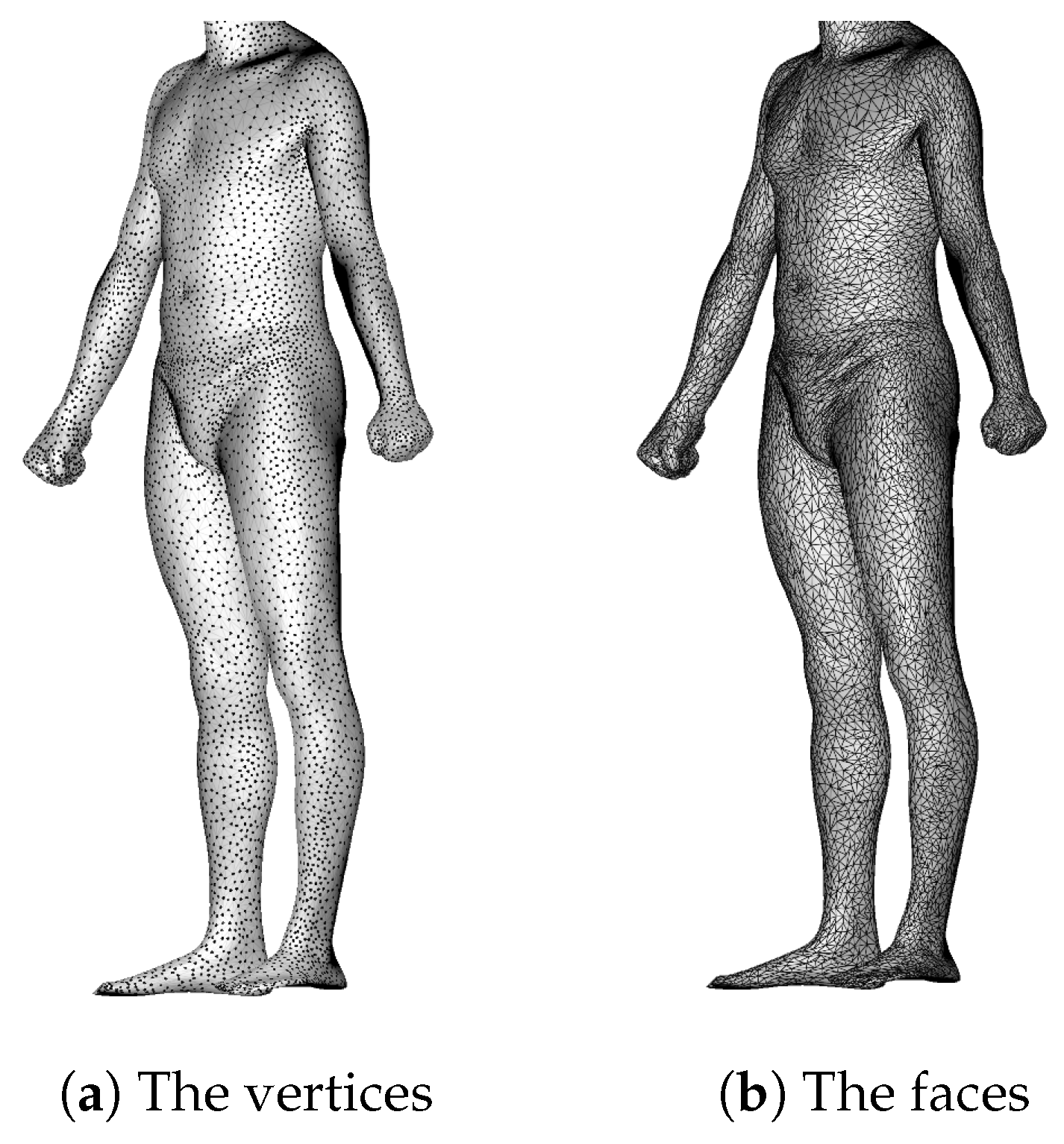
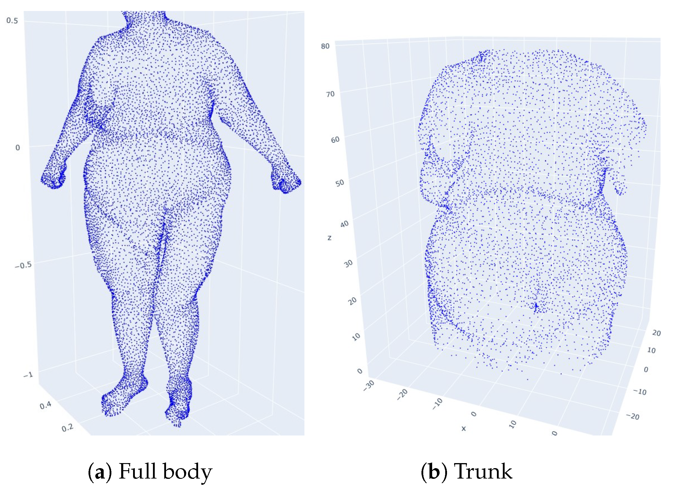
In this paper, we are using the dataset of [24], which is derived from the CAESAR dataset and is composed of 1517 male and 1531 female meshes, registered as OBJ files. Each mesh has 12,500 vertices (Figure 1a) and 25,000 faces (Figure 1b), and we extract and consider only the underlying point clouds of all the meshes. In the figures, the meshes and point clouds are presented headless for confidentiality. The individuals are numbered discontinuously from Spring0001 to Spring4800, and for convenience we refer to SpringXXXX by SXXXX.
2.2. Persistence Diagrams, Landscapes, Silhouettes and Distances
Persistent homology is a tool used to efficiently compute and encode the multidimensional homological features of topological spaces associated to a dataset. To compute these homological invariants, we have to build topological structures on the data such as filtered simplicial complexes.
A simplex is a notion generalizing points, line segments, triangles and tetrahedrons to any dimension and composed of faces that are also simplices of lower dimension. A simplicial complex K is a collection of simplices satisfying two properties: each face of a simplex of K is in K and the non-empty intersection of two simplices of K is a face of both of them. Given a body point cloud X in , several types of simplicial complexes can be constructed on X, such as the Vietoris–Rips and the Čech complexes. We center three-dimensional balls of radius on each data point, and we vary from 0 to . The data points are considered as 0-simplices, and when balls intersect, we add an n-dimensional face between them. The result is called a Čech complex. For each fixed , we count the homological features of the associated topological space. Since the underlying vector space is of dimension 3, we have three types of homological classes to consider:
- : The connected components;
- : The non-homotopic loops;
- : The two-dimensional voids.
Thus, we represent each homological feature by a point in , where its abscissa is the birth time of the feature and its ordinate is the death time. The set of points obtained in this way is the persistence diagram of X. The persistence barcode represents each homology class with a bar defined by its birth time, when the topological feature appears, and a death time, when the topological feature disappears. In order not to have too many points due to the creation and death of small homological features, a minimal persistence is fixed.
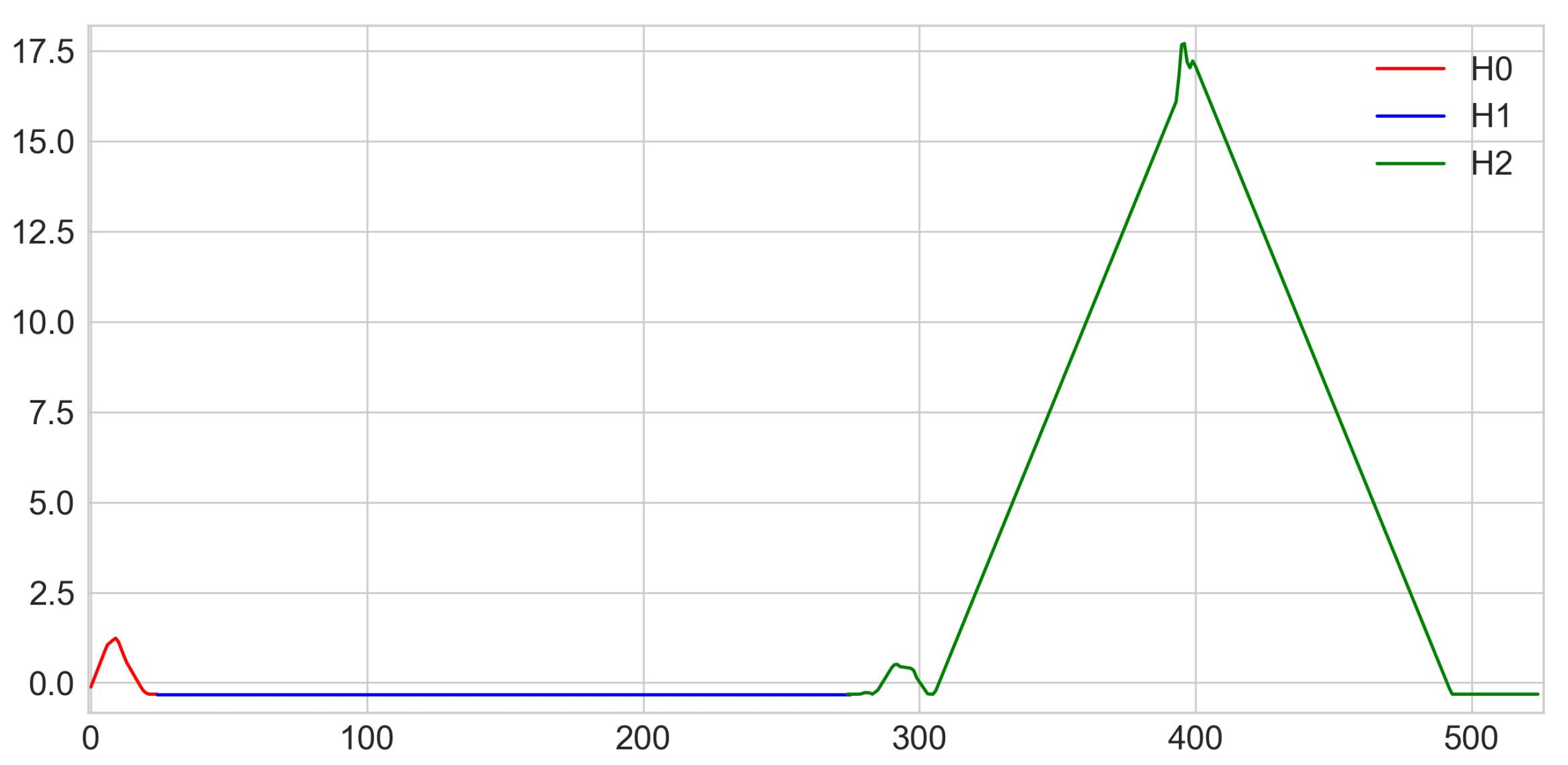
For example, in Figure 2, the persistence barcode and diagram of the individual S0013 (Figure 1) are given.
It is possible to compare persistence diagrams using the Wasserstein distance. Let D and be persistence diagrams. A perfect matching between D and is a subset such that every point of D and is exactly one time in , completing with the diagonal if necessary in order to ignore cardinality mismatches. The -Wasserstein distance between D and is defined by
where is the q-norm of x defined by
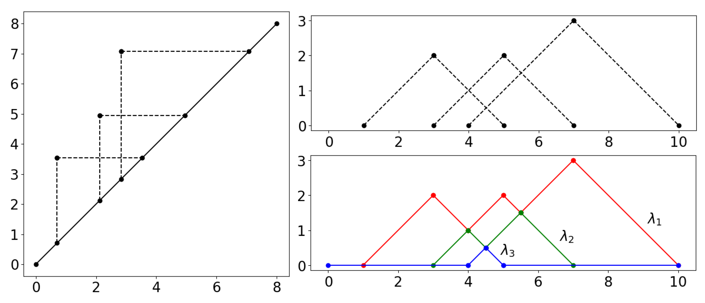
Persistence landscapes are an encoding of persistence diagrams by series of piecewise continuous linear functions [25,26]; see Figure 3. This allows us to perform statistics on them, the absence of which was a disadvantage of persistence diagrams. In particular, it is possible to calculate unique averages of landscapes. While a persistence landscape has a corresponding persistence diagram, an average of persistence landscapes does not.
A persistence silhouette is computed by taking a weighted average of the collection of 1D-piecewise-linear functions given by the persistence landscapes and then by evenly sampling this average on a given range. Finally, the corresponding vector of samples is returned; see Figure 4. For the implementation of clustering, we choose to make a vector consisting of 25 points of the silhouette of homologies, 250 points equidistant from the silhouette of homologies and 250 points equidistant from the silhouette of homologies for each persistence diagram. The points are the values of the silhouette equally spaced. Hence, each individual is represented by a vector in a real vector space of dimension 525 together with the Euclidean distance.
2.3. Interpretation of Persistent Homology
The persistence diagram of a body point cloud is composed of three types of homologies (see Figure 2). Since the points are distant from each other at an equivalent distance, all the balls are rapidly connected, thus giving a single connected component. Several and homologies representing the internal body cavities appear and disappear when the radius of the balls varies to . We now explain our approach to interpret and identify these homological features in terms of human anatomy. Since displaying the homologies in their entirety is too costly, we thought of other approaches for each degree.
For each homology, we know the radii of the balls at their birth and death. A simplex tree represents abstract simplicial complexes of any dimension. All faces of the simplicial complex are explicitly stored in a tree whose nodes are in bijection with the faces of the complex. This data structure allows us to efficiently implement a large range of basic operations on simplicial complexes. Using the simplex tree of a set of points, we know the values of the radii when pairs of points, triangles and tetrahedra are covered. The approach is slightly different depending on the dimension:
- Dimension 0: All homologies are born when the radius of the balls is zero. For each homology , we choose to display the second point of the pair covered at the birth of the homology as its representative.
- Dimension 1: First, we make an undirected graph containing all the points of a set, where each time a pair of points is covered, as the radius of the balls increases, we connect these points by an edge with a weight equal to the radius of the balls. At the birth of a homology , before adding the edge to our graph, we compute the shortest path connecting these two points, which we display by closing it with the segment connecting these points. The lace displayed is a likely representative of this homology. At the death of this homology, we recover the information of the triangle covered by the balls, and we add it to the display to give a general idea of the evolution of our homology.
- Dimension 2: For each homology , we simply display the triangle covered at its birth and the tetrahedron covered at its death.
For example, in the persistence diagram of the individual S0013 given in Figure 2, there are 13 different homologies numbered in the persistence barcode from 0 to 12. With this approach, we display each homology in Figure 5 and we can interpret them as follows:
- n°0: corresponding to the left part of the torso,
- n°1: corresponding to the right part of the torso,
- n°2: corresponding to a loop between legs at foot level,
- n°3: corresponding to a loop between legs from ankles to calves,
- n°4: corresponding to a loop between legs from knees to calves,
- n°5: corresponding to the head,
- n°6: corresponding to the right calf,
- n°7: corresponding to the left calf,
- n°8: corresponding to the right foot,
- n°9: corresponding to the whole body,
- n°10: corresponding to a loop around the right foot,
- n°11: corresponding to a loop around the left foot,
- n°12: of all the connected balls.
We remark that the arms and the left foot do not appear on the diagram. This is caused by the minimal persistence and the facts that the arms are too thin and that the scan of the left foot is more flat and deformed compared to the right one. Homology n°9 is particularly distinguished, and we call it the principal -homology. It corresponds to the aggregation of the parts and limbs of the body, thus forming the inner cavity of the body point cloud.
2.4. Normalization of Point Clouds by Homothety
We want morphotypes to be independent of the size of the individuals in order to propose a sizing system associated to each morphotype. For this purpose, we apply a homothety on each point cloud so that each individual is the same height: 1 m 70 cm. This affects the distances between them and individuals with similar morphology, but different heights become closer (Figure 6).
3. Anomaly Detection
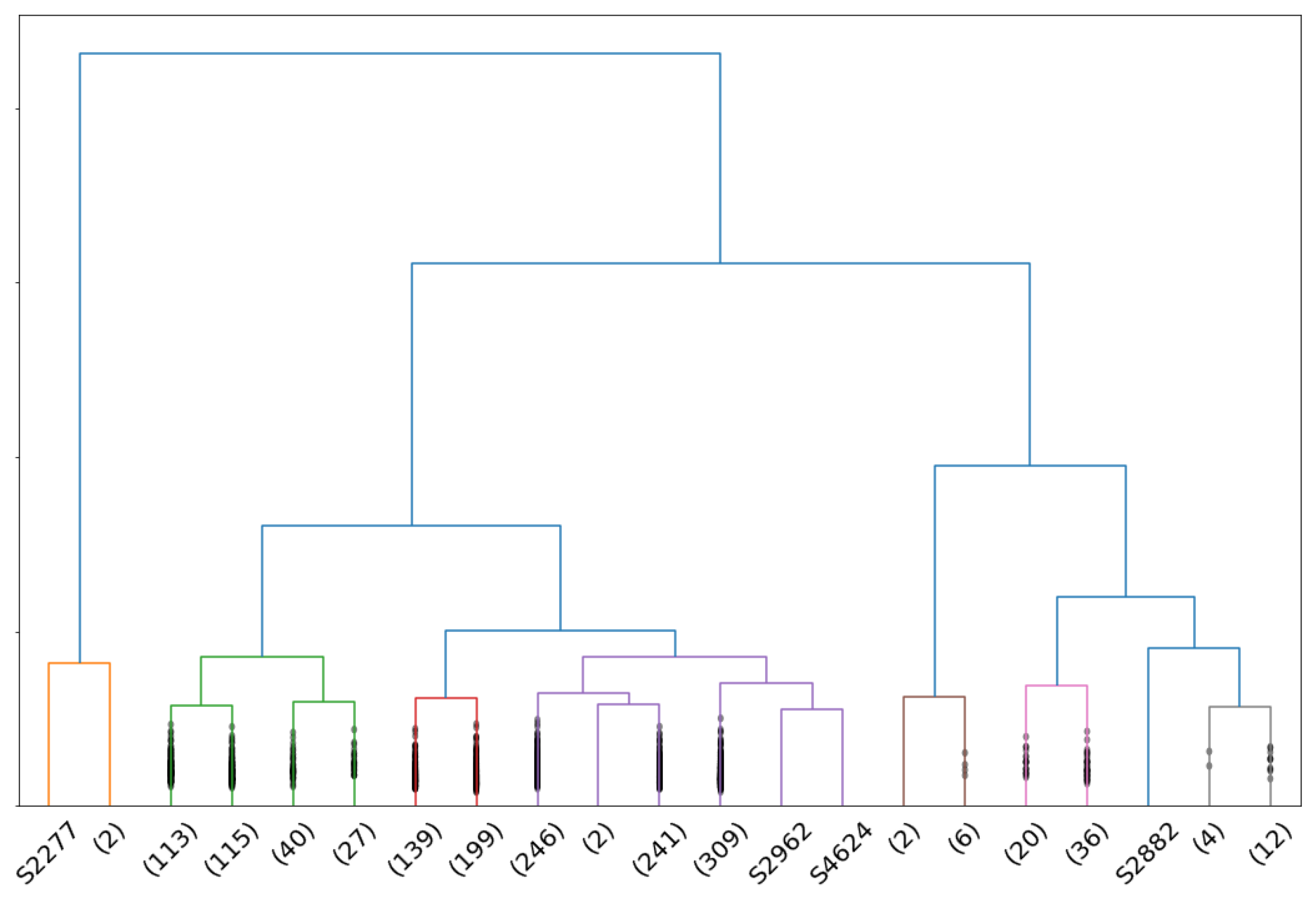
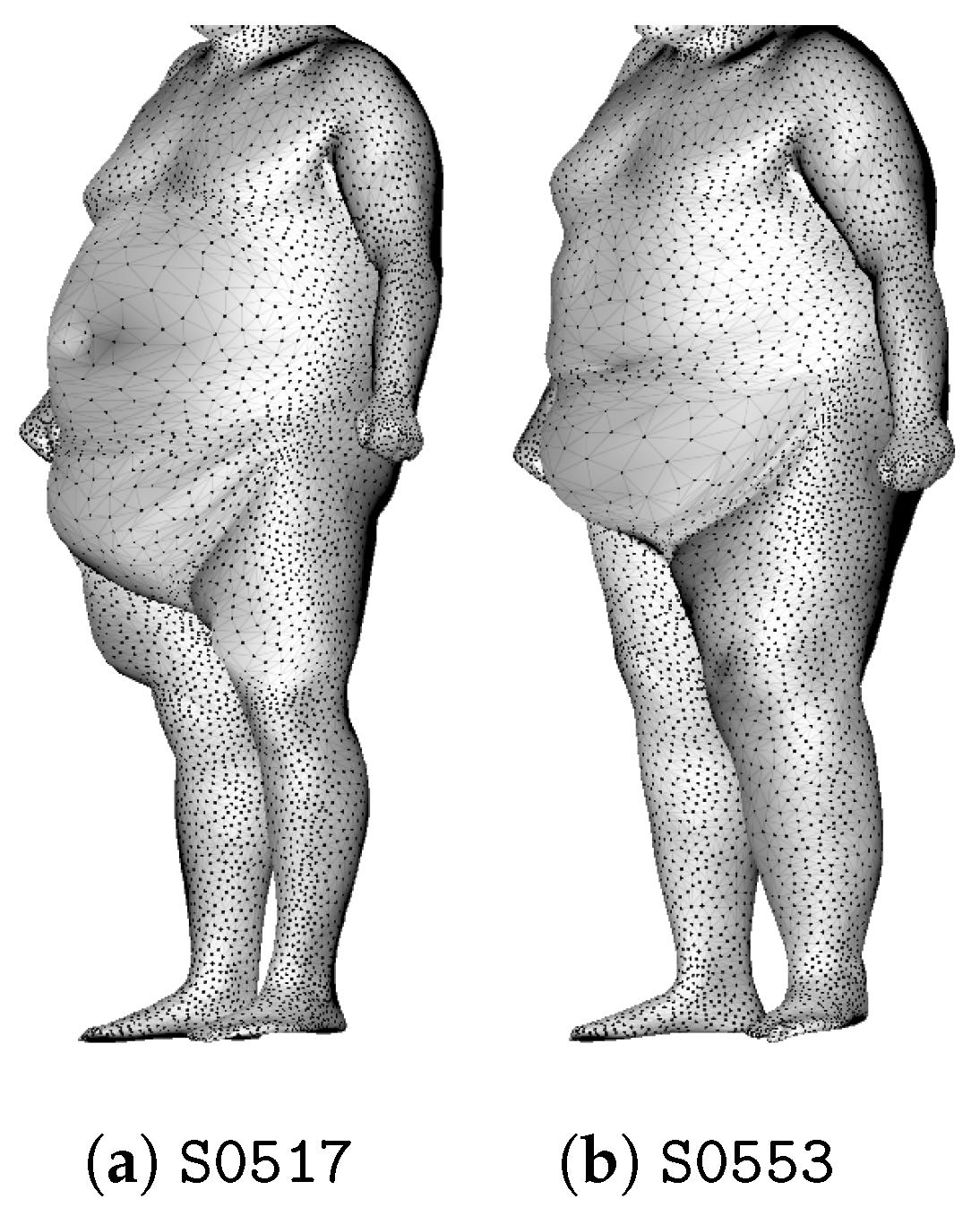
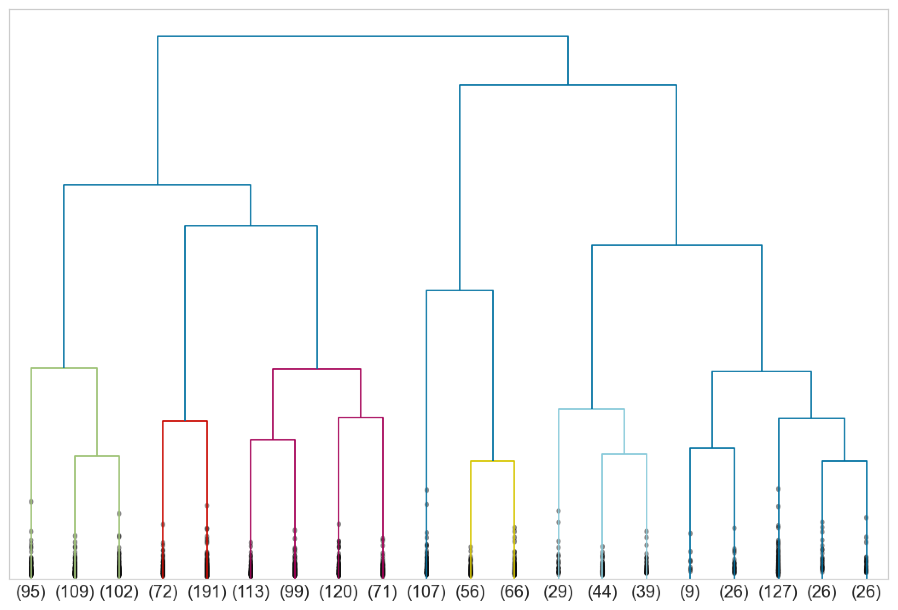
Among the data, there are anomalies of scans. We have found five anomalies for men and four for women. It turns out that they are encoded and detected by the persistence diagrams, Wasserstein distance and clustering algorithms. More precisely, we perform complete-linkage hierarchical clusterings on the persistence diagrams of the point clouds together with the Wasserstein distance (with ), separately for men and women. Analyzing corresponding truncated dendrograms, we remark that anomalies are very often isolated individuals agglomerating late. To find the best truncation of the dendrogram, we use as criteria the mean between the percentage of isolated individuals that are anomalies and the percentage of anomalies isolated in this way.
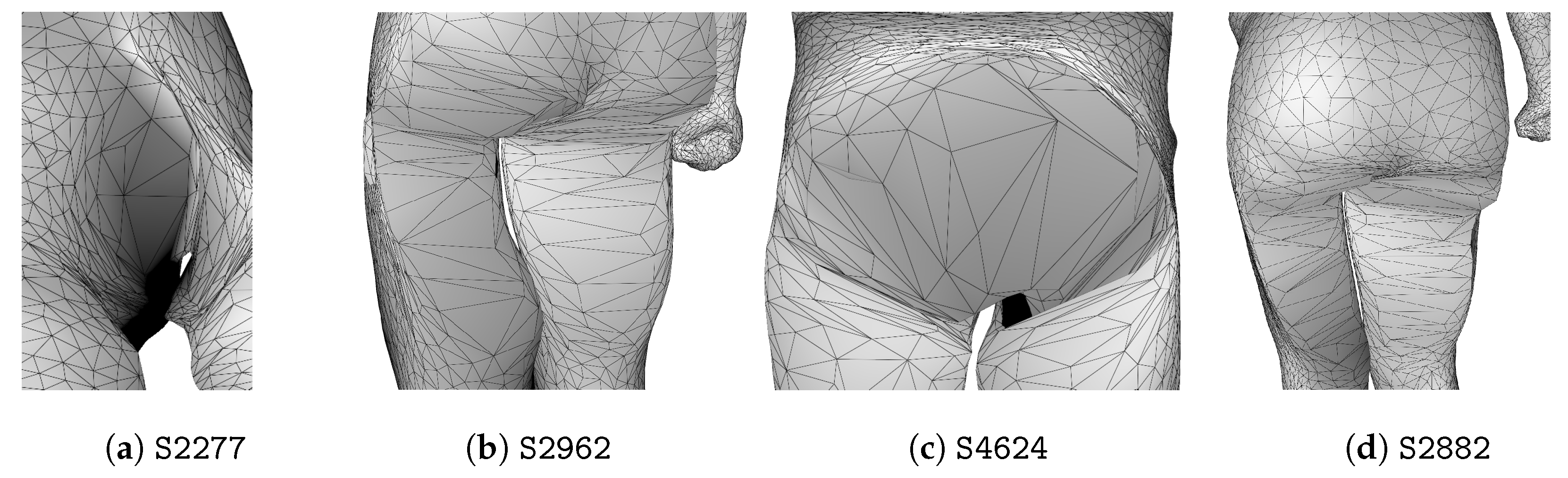
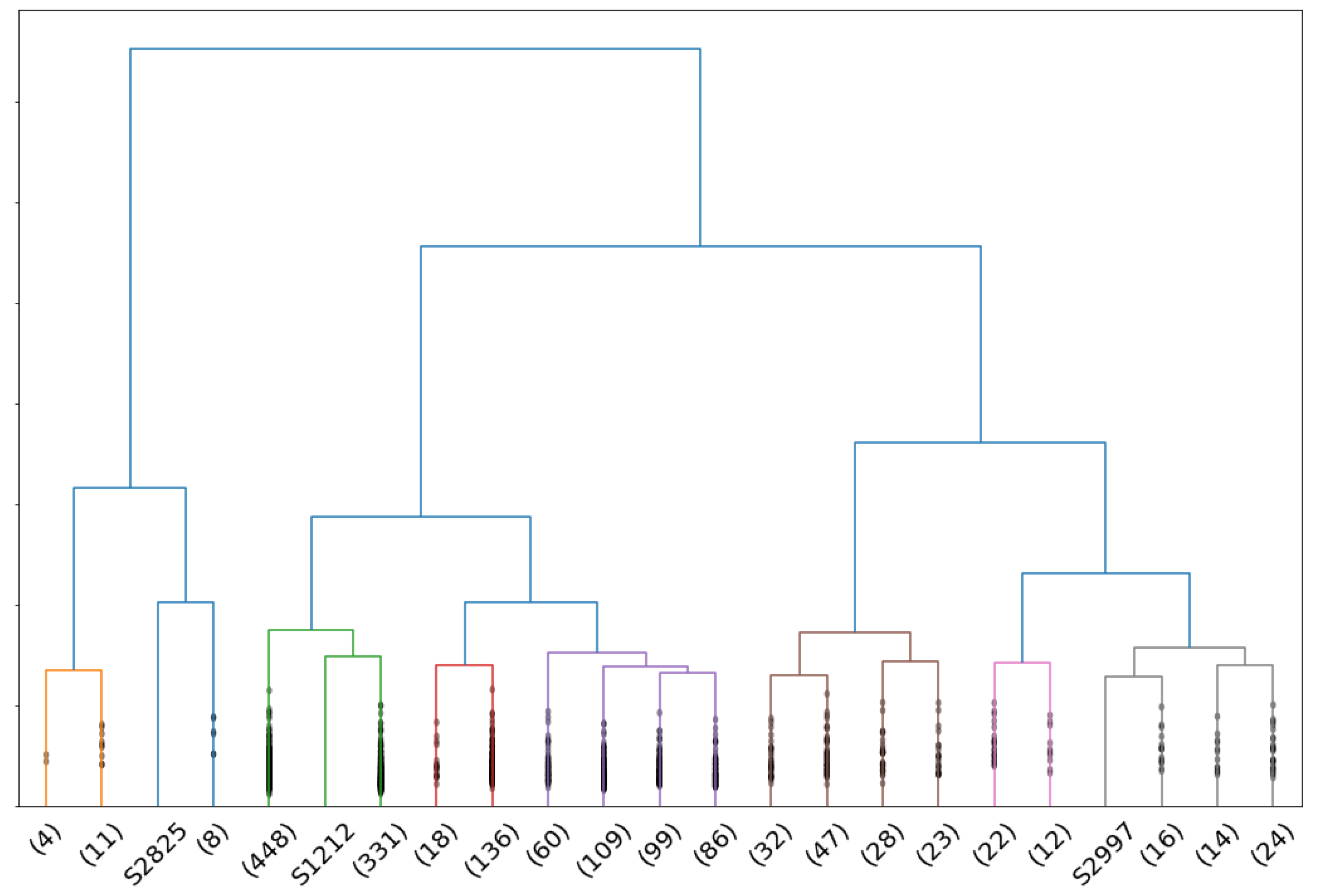
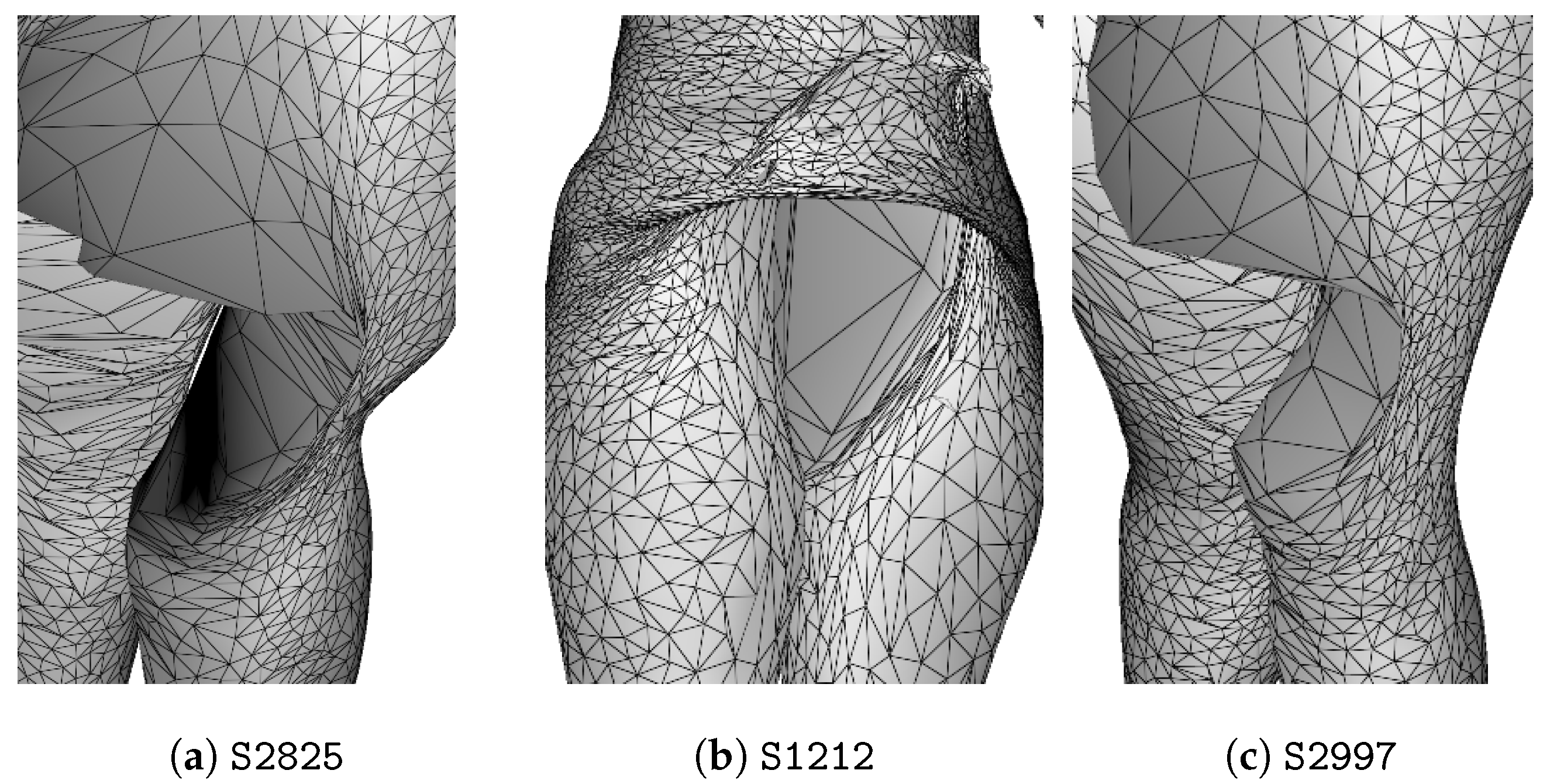
For men, the best truncation range is , where the criteria show that : of isolated individuals are anomalies and of anomalies are detected. Figure 7 shows the dendrogram for male point clouds truncated at 21 clusters, where the 4 isolated individuals are anomalies as shown in Figure 8.
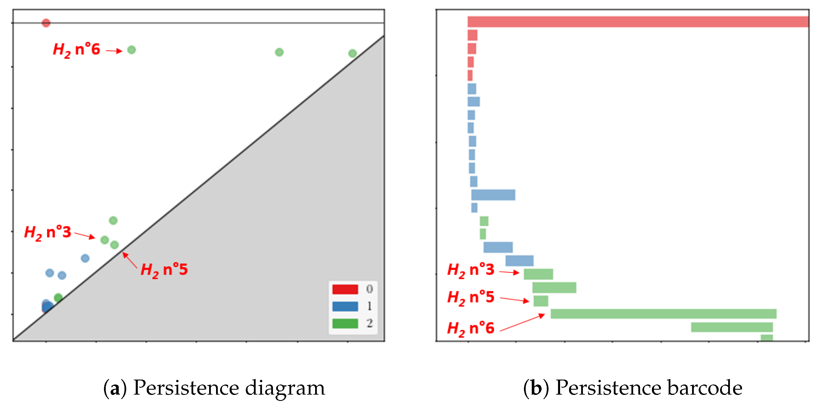
To illustrate that anomalies are detected by persistence, we analyze the persistence diagram of Figure 9, which corresponds to the individual S2962.
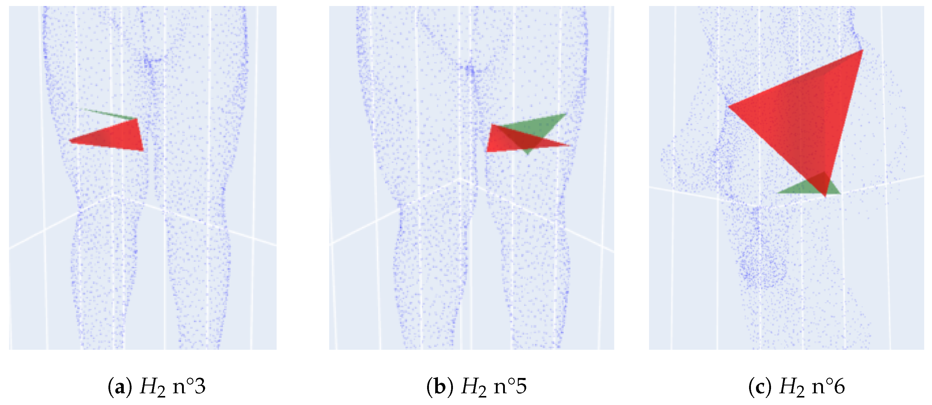
Its three homologies are particularly distinguished and can be seen at birth and death in Figure 10. Homologies numbers 3 and 5 correspond to the right and left leg, respectively, while the number 6 corresponds to the torso and is the principal -homology.
For normal scans, the principal -homology also aggregates legs. Because of the misplaced points and the holes on the point cloud, leg homologies are separated from the principal -homology which starts later than in the usual case.
4. Gender Discrimination Index
In this section, we analyze if clustering algorithms on persistence diagrams and silhouettes give groups separating men from women scans by changing the number of clusters. To this end, we use persistence diagrams or silhouettes, restricted to trunks of point clouds or not.
Let and be respectively the proportions of men and women in a cluster C. We have
where is the number of men in C, is the number of women in C and is the size of C. To measure the quality of a clustering of a set of mixed male and female diagrams or silhouettes , we introduce a gender discrimination index (GDI) defined by
where K is the number of clusters of , are the clusters of and is the number of elements in . Thus, the better the clustering separates men from women, the closer is to 1, and the worse it is, the closer is to 0. We can consider that a clustering is satisfactory to separate men from women if its GDI is greater or equal to .
4.1. Evolution of the GDI Score as a Function of the Number of Clusters
In this section, we observe the ability of different clustering methods to separate male from female persistence diagrams or silhouettes.
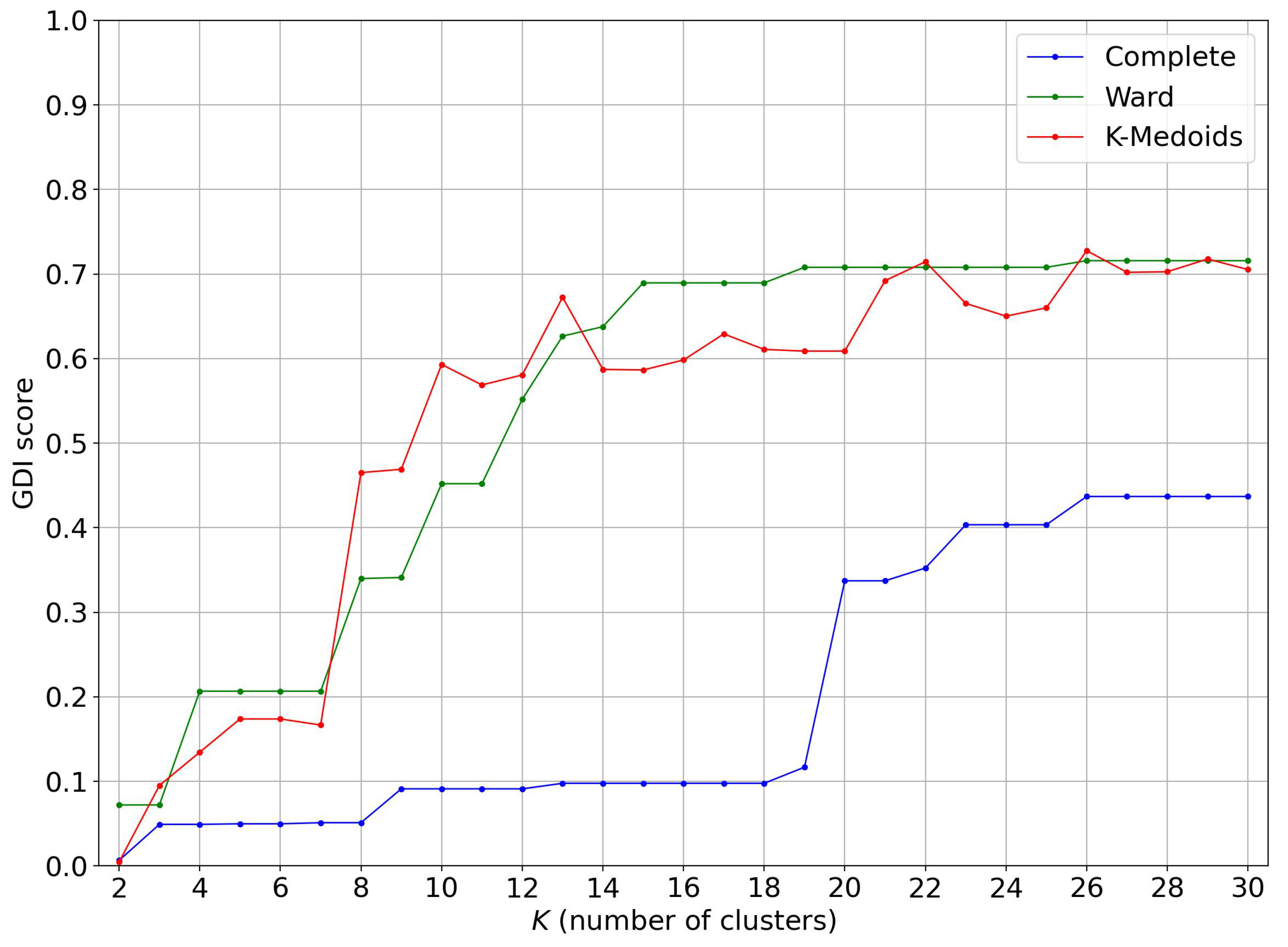
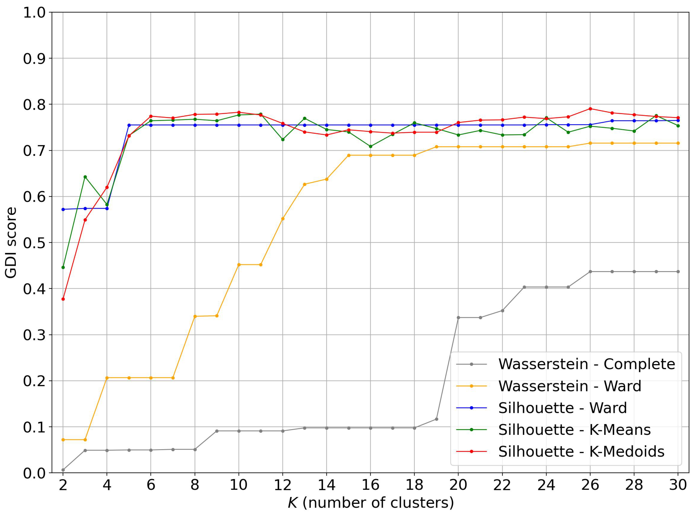
We use a matrix of Wasserstein distances between diagrams to perform hierarchical clustering with complete and Ward’s linkage methods [27] as well as K-Medoids clustering with the PAM (Partitioning Around Medoids) algorithm [28]. The notion of a barycenter between persistence diagrams is delicate [29,30], but we can use the Ward-linkage method with the Lance–Williams algorithm [31].
As shown in Figure 13, hierarchical clustering with the complete-linkage method does not differentiate correctly between female and male scans. However, the K-Medoids clustering has a correct GDI score for more than 10 clusters and becomes good on some occasions for more than 13 clusters. The Ward-linkage hierarchical clustering has a correct GDI score for more than 12 clusters and becomes good for more than 19 clusters.
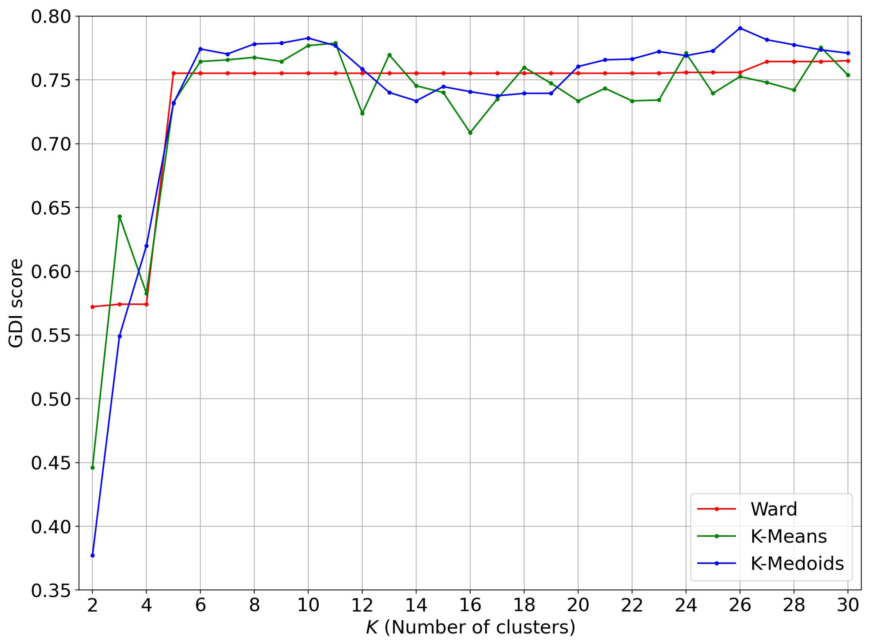
We now use vectors obtained from the silhouettes associated to the persistence diagrams of scans on which we perform a Ward-linkage hierarchical clustering as well as a K-Means clustering and a K-Medoids clustering with the PAM algorithm. This time, these three clustering algorithms give very good GDI scores; see Figure 14.
4.2. Restriction to Trunks
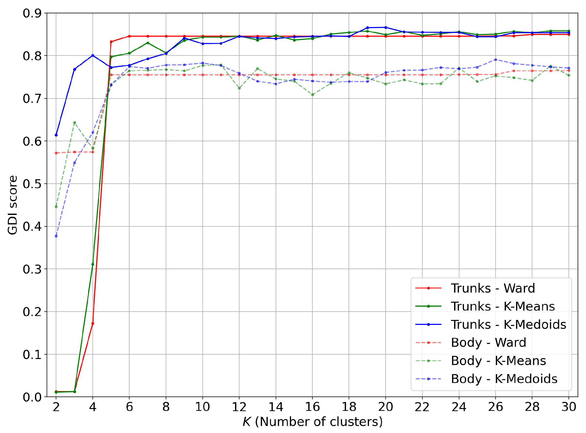
When constructing the silhouettes, we used a weighting that tended to favor the homologies corresponding to the trunks of the subjects, so the question then arises as to whether we would obtain better results by using only the points corresponding to the trunk of the body. To this end, we have developed an algorithm to isolate the points corresponding to the trunk of an individual which we now describe.
Let X be a normalized body point cloud at 1.70 m. We rotate and translate the scan such that the individual is standing along the height axis z and is at the minimal height of 0. Then, we isolate points located in the range cm to exclude points corresponding to the legs and head. We compute the director and intercept coefficients of two linear equations delimiting the trunk, taking into account the mean width of the individual. More precisely, we compute the lines and , which intersect at the height cm. Projecting the points on the plane , we obtain a set of points located between the first line, its symmetric with respect to the axis and below cm and a set of points located between the second line, its symmetric with respect to the axis and above cm. The union of and is composed of points of the individual’s trunk. In Figure 15, a body point cloud and the trunk point cloud isolated by this process are represented.
We now compare the clustering results using a Wasserstein distance matrix applied to the whole body and applied to the trunk.
From the curves in Figure 16 and the average GDI scores of Table 1, it appears that for clustering algorithms based on Wasserstein distances between persistence diagrams, it is not worth restricting these to trunk points.
We now compare the results of clustering algorithms using the vectors obtained from the persistence silhouettes applied to the whole body and applied to the trunk.
5. Human Body Shapes Classification
5.1. Male Morphotypes
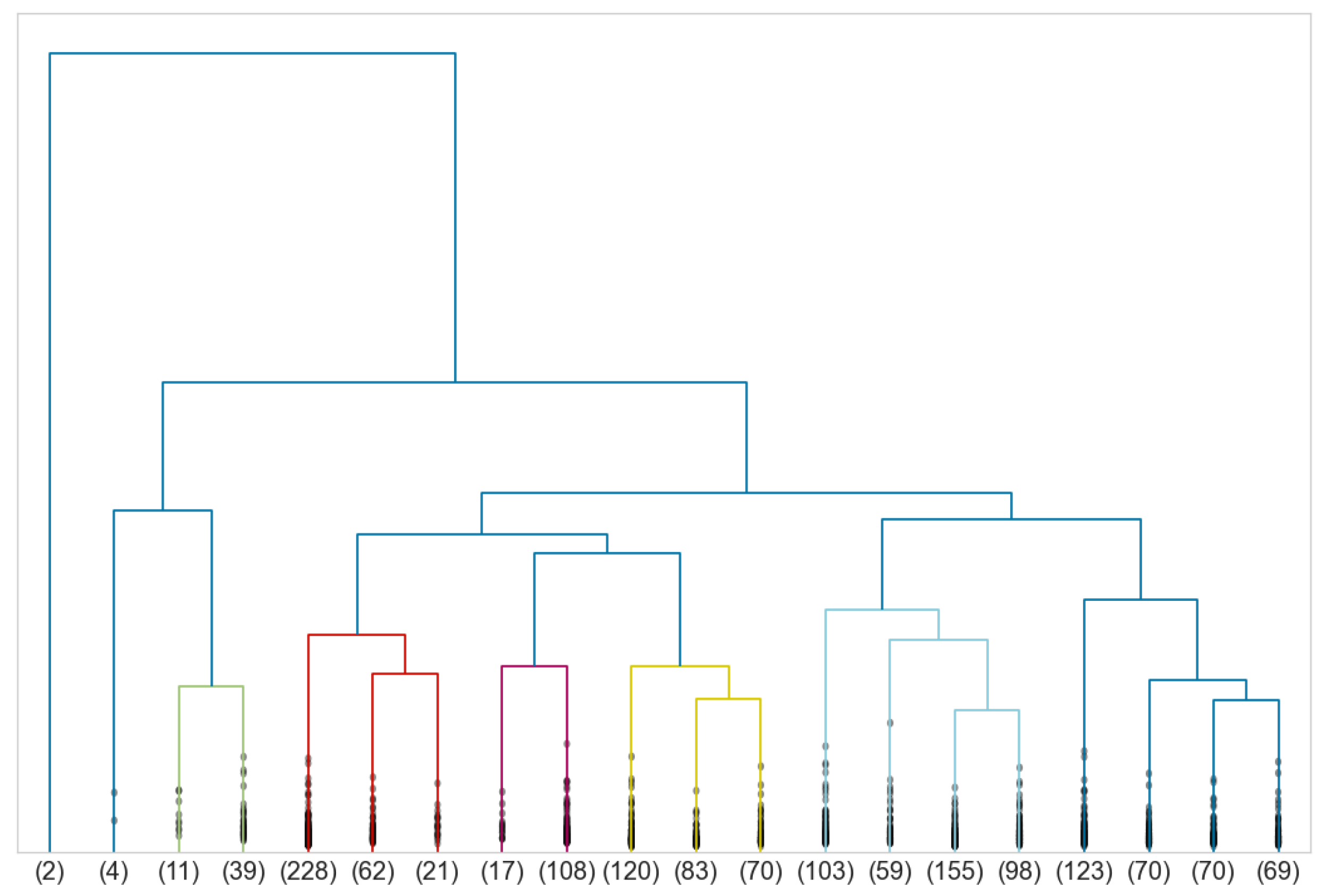
To define morphotypes of men’s body shapes, we perform a Ward-linkage hierarchical clustering on silhouettes of the persistence diagrams of the men’s point clouds together with the euclidean distance. The associated dendrogram is given in Figure 18.
To find a correct truncation of the dendrogram, we use the following clustering quality indices:
Since there is a continuity between human body shapes, there is no distinguished point common to all these indices. However, the Davies–Bouldin and Dunn indices both suggest to truncate at eight clusters. Information about size, mean distance of all pairs, diameter, mean distance to the mean and distance between the mean and the medoid of each cluster is given in Table 3.
The first cluster is only composed of two individuals who are extremely overweight, and their meshes are shown in Figure 19. The four men in the second cluster are also extremely overweight.
The medoid is the element minimizing the distance with other elements of the cluster. It can be considered as a representative, and we show in Figure 20 the medoids associated to every cluster, except for the first cluster.
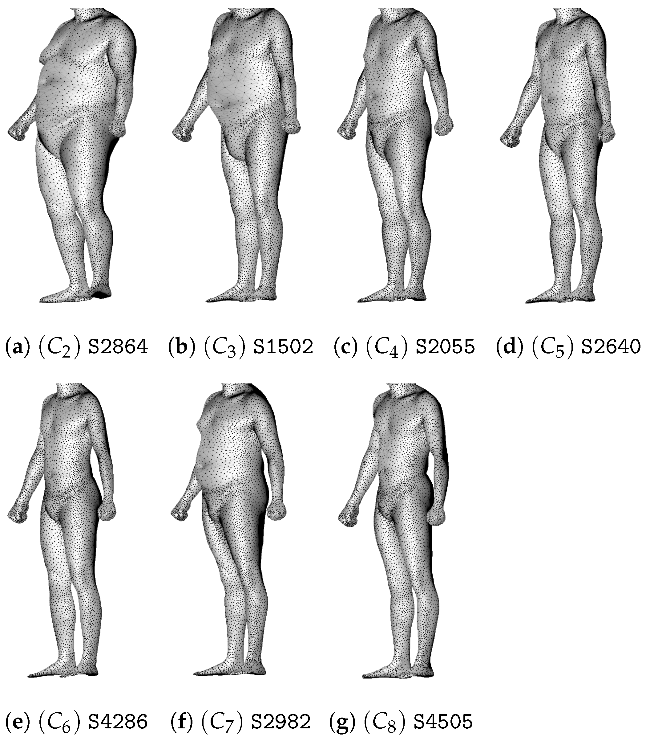
Since we do not have measurements associated with the individuals of the CAESAR database, in each group, we have to look at all the individuals in order to identify the predominant morphological features. It turns out that the clusters and are composed of overweight individuals of different categories, while the thinnest men are located in cluster . It turns out that individuals of clusters , and have a standard morphotype but that men of have a shorter torso than in and and that men of are more corpulent that in the two others.
5.2. Female Morphotypes
Similarly, to define morphotypes of women’s body shapes, we perform a Ward-linkage hierarchical clustering on silhouettes of the persistence diagrams of the women’s point clouds together with the euclidean distance. The associated dendrogram is given in Figure 21.
This time, the Silhouette and Dunn indices suggest truncating at seven clusters. Information about size, mean distance of all pairs, diameter, mean distance to the mean and distance between the mean and the medoid of each cluster is given in Table 4. Remark that clusters of women are more compact than clusters of men since the mean distance of pairs and diameter are much smaller.
We show in Figure 22 the medoids associated to the seven clusters.
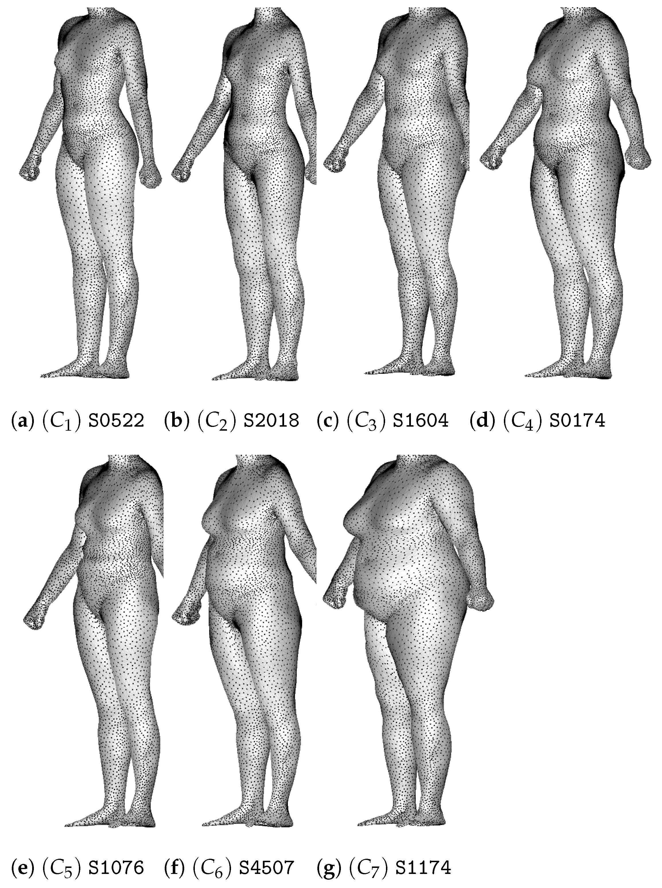
The first two clusters are composed of thin women, but in the first one, they have a shorter torso with a waist circumference that is more pronounced. The clusters and are composed of overweight individuals of different categories. The women of the clusters have a straight body without much difference between waist, hip and chest circumferences. Individuals of and have a larger hip circumference compared to the waist circumference, but women of have a stronger lower body while women of have a shorter torso.
6. Discussion
The research conducted in this paper demonstrates that the tools of topological data analysis and persistence theory permit us to extract pertinent information about the shape of anthropometric point clouds. The homologies of the persistence diagram of human body points have interesting interpretations in terms of human anatomy. Hence, most of the scan anomalies are correctly detected by clustering algorithms. The gender discrimination index shows that it is worth restricting our search to trunk body points to separate men from women and that the Ward-linkage hierarchical clustering and the K-Medoids clustering give better results than the complete-linkage hierarchical clustering. Finally, we obtain eight morphotypes of men and seven morphotypes of women’s body shapes with Ward-linkage hierarchical clusterings. The clusters are composed of individuals of similar weight classes, and the groups can be distinguished by their ratios between bust, waist and hip circumferences or by their torso sizes or their lower body shapes. It is worth noting that the female clusters have better proportions and smaller diameters than the male clusters.
The proposed approach is promising for anomaly detection and classification and should be applied to other types of point clouds in different contexts. The method can also be extended to other problems related to human bodies, such as measurement extraction with supervised machine learning algorithms.
Author Contributions
Conceptualization, S.d.R., P.M. and F.B.; methodology, S.d.R., P.M. and F.B.; formal analysis, S.d.R. and P.M.; software, S.d.R. and P.M.; writing—original draft preparation, S.d.R. and P.M.; writing—review and editing, S.d.R. and P.M.; visualization, S.d.R. and P.M.; supervision, P.M. and F.B. All authors have read and agreed to the published version of the manuscript.
Funding
This work was supported by Labcom-DiTeX, a joint research group in Textile Data Innovation between Institut Français du Textile et de l’Habillement (IFTH) and Université de Technologie de Troyes (UTT).
Institutional Review Board Statement
Not applicable.
Informed Consent Statement
Not applicable.
Data Availability Statement
The data used in this article come from [24].
Conflicts of Interest
The authors declare no conflict of interest.
References
- Simmons, K.; Istook, C.; Devarajan, P. Female Figure Identification Technique (FFIT) for apparel part I: Describing female shapes. J. Text. Appar. Technol. Manag. 2004, 4, 1–16. [Google Scholar]
- Song, H.K.; Ashdown, S. Categorization of lower body shapes for adult females based on multiple view analysis. Text. Res. J. 2011, 81, 914–931. [Google Scholar] [CrossRef]
- Nakamura, K.; Kurokawa, T. Analysis and classification of three-dimensional trunk shape of women by using the human body shape model. Int. J. Comput. Appl. Technol. 2009, 34, 278–284. [Google Scholar] [CrossRef] [Green Version]
- Cottle, F.S. Statistical Human Body Form Classification: Methodology Development and Application; Auburn University: Auburn, AL, USA, 2012. [Google Scholar]
- Hamad, M.; Thomassey, S.; Bruniaux, P. A new sizing system based on 3D morphology clustering. Comput. Ind. Eng. 2017, 113, 683–692. [Google Scholar] [CrossRef]
- Naveed, T.; Zhong, Y.; Hussain, A.; Babar, A.A.; Naeem, A.; Iqbal, A.; Saleemi, S. Female Body Shape Classifications and Their Significant Impact on Fabric Utilization. Fibers Polym. 2018, 19, 2642–2656. [Google Scholar] [CrossRef]
- Pei, J.; Park, H.; Ashdown, S.P. Female breast shape categorization based on analysis of CAESAR 3D body scan data. Text. Res. J. 2019, 89, 590–611. [Google Scholar] [CrossRef]
- Chazal, F.; Michel, B. An Introduction to Topological Data Analysis: Fundamental and Practical Aspects for Data Scientists. Front. Artif. Intell. 2021, 4, 667963. [Google Scholar] [CrossRef] [PubMed]
- Munch, E. A User’s Guide to Topological Data Analysis. J. Learn. Anal. 2017, 4, 47–61. [Google Scholar] [CrossRef] [Green Version]
- Edelsbrunner, H.; Letscher, D.; Zomorodian, A. Topological Persistence and Simplification. Discret. Comput. Geom. 2002, 28, 511–533. [Google Scholar] [CrossRef] [Green Version]
- Zomorodian, A.; Carlsson, G. Computing Persistent Homology. Discret. Comput. Geom. 2005, 33, 249–274. [Google Scholar] [CrossRef] [Green Version]
- Cohen-Steiner, D.; Edelsbrunner, H.; Harer, J. Stability of Persistence Diagrams. In Proceedings of the SCG ’05: Twenty-First Annual Symposium on Computational Geometry, Pisa, Italy, 6–8 June 2005; Association for Computing Machinery: New York, NY, USA, 2005; pp. 263–271. [Google Scholar] [CrossRef]
- Chazal, F.; Cohen-Steiner, D.; Glisse, M.; Guibas, L.J.; Oudot, S.Y. Proximity of Persistence Modules and Their Diagrams. In Proceedings of the SCG ’09: Twenty-Fifth Annual Symposium on Computational Geometry, Aarhus, Denmark, 8–10 June 2009; Association for Computing Machinery: New York, NY, USA, 2009; pp. 237–246. [Google Scholar] [CrossRef] [Green Version]
- Umeda, Y.; Kaneko, J.; Kikuchi, H. Topological data analysis and its application to time-series data analysis. Fujitsu Sci. Tech. J. 2019, 55, 65–71. [Google Scholar]
- Li, C.; Ovsjanikov, M.; Chazal, F. Persistence-Based Structural Recognition. In Proceedings of the 2014 IEEE Conference on Computer Vision and Pattern Recognition, Columbus, OH, USA, 23–28 June 2014; pp. 2003–2010. [Google Scholar] [CrossRef] [Green Version]
- Horak, D.; Maletić, S.; Rajković, M. Persistent homology of complex networks. J. Stat. Mech. Theory Exp. 2009, 2009, P03034. [Google Scholar] [CrossRef] [Green Version]
- Yao, Y.; Sun, J.; Huang, X.; Bowman, G.R.; Singh, G.; Lesnick, M.; Guibas, L.J.; Pande, V.S.; Carlsson, G. Topological methods for exploring low-density states in biomolecular folding pathways. J. Chem. Phys. 2009, 130, 144115. [Google Scholar] [CrossRef] [Green Version]
- Skaf, Y.; Laubenbacher, R. Topological data analysis in biomedicine: A review. J. Biomed. Inform. 2022, 130, 104082. [Google Scholar] [CrossRef]
- Corcoran, P.; Jones, C.B. Topological data analysis for geographical information science using persistent homology. Int. J. Geogr. Inf. Sci. 2023, 37, 712–745. [Google Scholar] [CrossRef]
- Ver Hoef, L.; Adams, H.; King, E.J.; Ebert-Uphoff, I. A Primer on Topological Data Analysis to Support Image Analysis Tasks in Environmental Science. Artif. Intell. Earth Syst. 2023, 2, e220039. [Google Scholar] [CrossRef]
- Mahmmod, B.M.; Abdulhussain, S.H.; Suk, T.; Hussain, A. Fast computation of Hahn polynomials for high order moments. IEEE Access 2022, 10, 48719–48732. [Google Scholar] [CrossRef]
- Jassim, W.A.; Raveendran, P.; Mukundan, R. New orthogonal polynomials for speech signal and image processing. IET Signal Process. 2012, 6, 713–723. [Google Scholar] [CrossRef]
- Abdulhussain, S.H.; Mahmmod, B.M.; Baker, T.; Al-Jumeily, D. Fast and accurate computation of high-order Tchebichef polynomials. Concurr. Comput. Pract. Exp. 2022, 34, e7311. [Google Scholar] [CrossRef]
- Yang, Y.; Yu, Y.; Zhou, Y.; Du, S.; Davis, J.; Yang, R. Semantic Parametric Reshaping of Human Body Models. In Proceedings of the 2014 2nd International Conference on 3D Vision, Tokyo, Japan, 8–11 December 2014; Volume 2, pp. 41–48. [Google Scholar] [CrossRef]
- Chazal, F.; Fasy, B.T.; Lecci, F.; Rinaldo, A.; Wasserman, L. Stochastic Convergence of Persistence Landscapes and Silhouettes. In Proceedings of the SOCG’14: Thirtieth Annual Symposium on Computational Geometry, Kyoto, Japan, 8–11 June 2014; Association for Computing Machinery: New York, NY, USA, 2014; pp. 474–483. [Google Scholar] [CrossRef] [Green Version]
- Bubenik, P. Statistical Topological Data Analysis Using Persistence Landscapes. J. Mach. Learn. Res. 2015, 16, 77–102. [Google Scholar]
- Ward, J.H.W., Jr. Hierarchical Grouping to Optimize an Objective Function. J. Am. Stat. Assoc. 1963, 58, 236–244. [Google Scholar] [CrossRef]
- Kaufman, L.; Rousseeuw, P.J. Partitioning around Medoids (Program PAM). In Finding Groups in Data; John Wiley & Sons, Ltd.: Hoboken, NJ, USA, 1990. [Google Scholar] [CrossRef]
- Mileyko, Y.; Mukherjee, S.; Harer, J. Probability measures on the space of persistence diagrams. Inverse Probl. 2011, 27, 124007. [Google Scholar] [CrossRef] [Green Version]
- Turner, K.; Mileyko, Y.; Mukherjee, S.; Harer, J. Frechet Means for Distributions of Persistence Diagrams. Discret. Comput. Geom. 2014, 52, 44–70. [Google Scholar] [CrossRef] [Green Version]
- Lance, G.N.; Williams, W.T. A general theory of classificatory sorting strategies: II. Clustering systems. Comput. J. 1967, 10, 271–277. [Google Scholar] [CrossRef] [Green Version]
- Davies, D.L.; Bouldin, D.W. A Cluster Separation Measure. IEEE Trans. Pattern Anal. Mach. Intell. 1979, PAMI-1, 224–227. [Google Scholar] [CrossRef]
- Rousseeuw, P.J. Silhouettes: A graphical aid to the interpretation and validation of cluster analysis. J. Comput. Appl. Math. 1987, 20, 53–65. [Google Scholar] [CrossRef] [Green Version]
- Dunn, J.C. A Fuzzy Relative of the ISODATA Process and Its Use in Detecting Compact Well-Separated Clusters. J. Cybern. 1973, 3, 32–57. [Google Scholar] [CrossRef]
Figure 1.
The mesh of the individual S0013.

Figure 2.
The persistence diagram and barcode of S0013.

Figure 3.
Visual explanation of persistence landscapes. The persistence diagram (left) is tilted so that the diagonal becomes the new horizontal axis (top right). The are the piecewise linear functions (bottom right).
Figure 3.
Visual explanation of persistence landscapes. The persistence diagram (left) is tilted so that the diagonal becomes the new horizontal axis (top right). The are the piecewise linear functions (bottom right).

Figure 4.
Representation of a vector obtained by persistence silhouette.

Figure 5.
All non homologies of the persistence diagram of S0013.

Figure 6.
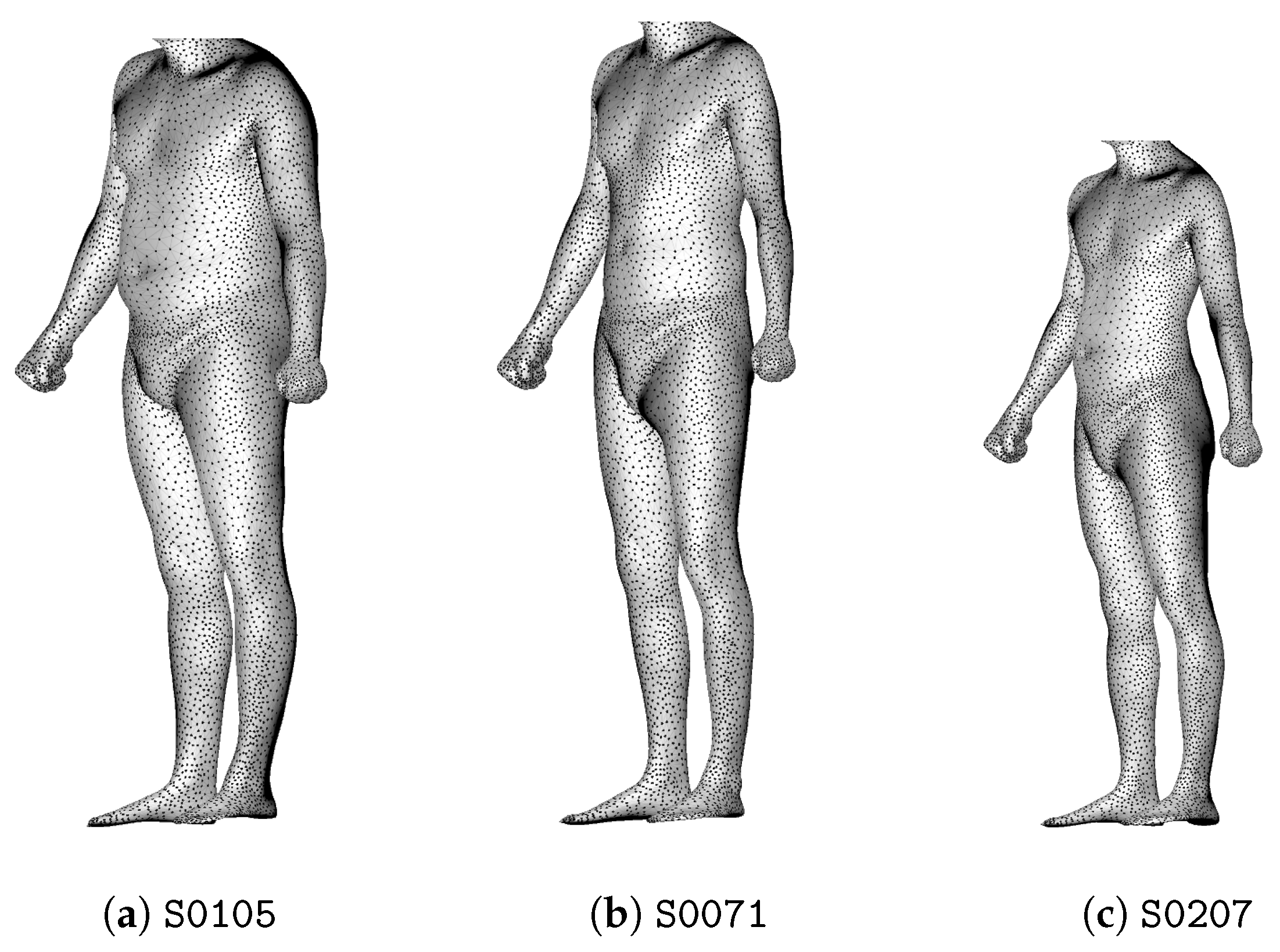
Individuals (a–c) are 1.89 m, 1.93 m and 1.65 m tall, respectively. Among them, the couple (a,b) is the closest before normalization, and the couple (b,c) is the closest after normalization.
Figure 6.
Individuals (a–c) are 1.89 m, 1.93 m and 1.65 m tall, respectively. Among them, the couple (a,b) is the closest before normalization, and the couple (b,c) is the closest after normalization.

Figure 7.
Dendrogram associated to a complete-linkage hierarchical clustering of the persistence diagrams of male point clouds with the Wasserstein distance. Clusters composed of one individual are presented without parentheses.
Figure 7.
Dendrogram associated to a complete-linkage hierarchical clustering of the persistence diagrams of male point clouds with the Wasserstein distance. Clusters composed of one individual are presented without parentheses.

Figure 8.
Anomalies of men scans detected by complete-linkage hierarchical clustering of persistence diagrams.
Figure 8.
Anomalies of men scans detected by complete-linkage hierarchical clustering of persistence diagrams.

Figure 9.
Persistence diagram and barcode of the anomaly of scan S2962. Three particular homologies reflecting the anomaly are highlighted.
Figure 9.
Persistence diagram and barcode of the anomaly of scan S2962. Three particular homologies reflecting the anomaly are highlighted.

Figure 10.
Three abnormal homologies at birth and death of the defective scan S2962.

Figure 11.
Dendrogram associated to a complete-linkage hierarchical clustering of the persistence diagrams of female point clouds with the Wasserstein distance.
Figure 11.
Dendrogram associated to a complete-linkage hierarchical clustering of the persistence diagrams of female point clouds with the Wasserstein distance.

Figure 12.
Anomalies of female scans detected by complete-linkage hierarchical clustering of persistence diagrams.
Figure 12.
Anomalies of female scans detected by complete-linkage hierarchical clustering of persistence diagrams.

Figure 13.
GDI score evolution of various clustering algorithms on the persistence diagrams with Wasserstein distance.
Figure 13.
GDI score evolution of various clustering algorithms on the persistence diagrams with Wasserstein distance.

Figure 14.
GDI score evolution of various clustering algorithms on the persistence silhouettes.

Figure 15.
An individual and its isolated trunk.

Figure 16.
Comparison of GDI score on the persistence diagrams of the whole body and the trunk with the Wasserstein distance.
Figure 16.
Comparison of GDI score on the persistence diagrams of the whole body and the trunk with the Wasserstein distance.

Figure 17.
Comparison of GDI score on the persistence silhouettes of the whole body and the trunk.

Figure 18.
Dendrogram associated to a Ward-linkage hierarchical clustering of the silhouettes of the persistence diagrams of male point clouds.
Figure 18.
Dendrogram associated to a Ward-linkage hierarchical clustering of the silhouettes of the persistence diagrams of male point clouds.

Figure 19.
The two individuals of cluster .

Figure 20.
Medoids of clusters to of the Ward-linkage hierarchical clustering.

Figure 21.
Dendrogram associated to a Ward-linkage hierarchical clustering of the silhouettes of the persistence diagrams of female point clouds.
Figure 21.
Dendrogram associated to a Ward-linkage hierarchical clustering of the silhouettes of the persistence diagrams of female point clouds.

Figure 22.
Medoids of the seven clusters of the Ward-linkage hierarchical clustering.


Table 1.
Average GDI scores on the persistence diagrams of the whole body and the trunk with the Wasserstein distance.
Table 1.
Average GDI scores on the persistence diagrams of the whole body and the trunk with the Wasserstein distance.
| Complete | Ward | K-Medoids | |
|---|---|---|---|
| Body | 0.2 | 0.54 | 0.526 |
| Trunk | 0.21 | 0.553 | 0.582 |
Table 2.
Average GDI scores on the persistence silhouettes of the whole body and the trunk.
| Ward | K-Means | K-Medoids | |
|---|---|---|---|
| Body | 0.738 | 0.73 | 0.737 |
| Trunk | 0.765 | 0.767 | 0.827 |
Table 3.
Clustering of male body shapes.
| Cluster | ||||||||
|---|---|---|---|---|---|---|---|---|
| Size | 2 | 4 | 50 | 311 | 125 | 273 | 415 | 332 |
| Proportion (in percent) | 0.1 | 0.3 | 3 | 21 | 8 | 18 | 27 | 22 |
| Mean distance | 79.6 | 39.4 | 28.6 | 17.4 | 20.3 | 16.3 | 18.9 | 19.4 |
| Diameter | 79.6 | 53.9 | 62 | 49.6 | 59.2 | 54.6 | 67.1 | 69.4 |
| Distance to the mean | 39.8 | 24.4 | 19.6 | 12.1 | 14.2 | 11.5 | 13.1 | 13.6 |
| Distance mean–medoid | 39.8 | 20.1 | 9 | 3.4 | 5.9 | 6.9 | 5.1 | 6.1 |
Table 4.
Clustering of female body shapes.
| Clusters | |||||||
|---|---|---|---|---|---|---|---|
| Size | 306 | 263 | 403 | 107 | 122 | 112 | 214 |
| Proportion (in percent) | 20 | 17 | 27 | 7 | 8 | 7 | 14 |
| Mean distance | 14.2 | 12.7 | 14.1 | 14.3 | 14 | 19 | 21.3 |
| Diameter | 36.6 | 32 | 32.1 | 31.9 | 38.2 | 59.3 | 62.4 |
| Distance to the mean | 10.1 | 9 | 10.1 | 10.1 | 9.9 | 13.3 | 14.8 |
| Distance mean–medoid | 3.4 | 3.4 | 4.5 | 3.3 | 3.6 | 5.9 | 5.2 |
Disclaimer/Publisher’s Note: The statements, opinions and data contained in all publications are solely those of the individual author(s) and contributor(s) and not of MDPI and/or the editor(s). MDPI and/or the editor(s) disclaim responsibility for any injury to people or property resulting from any ideas, methods, instructions or products referred to in the content. |
© 2023 by the authors. Licensee MDPI, Basel, Switzerland. This article is an open access article distributed under the terms and conditions of the Creative Commons Attribution (CC BY) license (https://creativecommons.org/licenses/by/4.0/).
Share and Cite
MDPI and ACS Style
de Rose, S.; Meyer, P.; Bertrand, F. Human Body Shapes Anomaly Detection and Classification Using Persistent Homology. Algorithms 2023, 16, 161. https://doi.org/10.3390/a16030161
AMA Style
de Rose S, Meyer P, Bertrand F. Human Body Shapes Anomaly Detection and Classification Using Persistent Homology. Algorithms. 2023; 16(3):161. https://doi.org/10.3390/a16030161
Chicago/Turabian Stylede Rose, Steve, Philippe Meyer, and Frédéric Bertrand. 2023. "Human Body Shapes Anomaly Detection and Classification Using Persistent Homology" Algorithms 16, no. 3: 161. https://doi.org/10.3390/a16030161
Note that from the first issue of 2016, this journal uses article numbers instead of page numbers. See further details here.