

Implementing Deep Convolutional Neural Networks for QR Code-Based Printed Source Identification

Institute of Information Management, National Yang Ming Chiao Tung University, 1001 Ta-Hsueh Road, Hsin-Chu 300, Taiwan
*
Author to whom correspondence should be addressed.
Algorithms 2023, 16(3), 160; https://doi.org/10.3390/a16030160
Submission received: 15 January 2023
/
Revised: 12 February 2023
/
Accepted: 2 March 2023
/
Published: 14 March 2023
(This article belongs to the Special Issue Deep Neural Networks and Optimization Algorithms)
Abstract
:QR codes (short for Quick Response codes) were originally developed for use in the automotive industry to track factory inventories and logistics, but their popularity has expanded significantly in the past few years due to the widespread applications of smartphones and mobile phone cameras. QR codes can be used for a variety of purposes, including tracking inventory, advertising, electronic ticketing, and mobile payments. Although they are convenient and widely used to store and share information, their accessibility also means they might be forged easily. Digital forensics can be used to recognize direct links of printed documents, including QR codes, which is important for the investigation of forged documents and the prosecution of forgers. The process involves using optical mechanisms to identify the relationship between source printers and the duplicates. Techniques regarding computer vision and machine learning, such as convolutional neural networks (CNNs), can be implemented to study and summarize statistical features in order to improve identification accuracy. This study implemented AlexNet, DenseNet201, GoogleNet, MobileNetv2, ResNet, VGG16, and other Pretrained CNN models for evaluating their abilities to predict the source printer of QR codes with a high level of accuracy. Among them, the customized CNN model demonstrated better results in identifying printed sources of grayscale and color QR codes with less computational power and training time.
1. Introduction
QR codes have been a popular and convenient way to store and share information, including URLs, for a certain period of time. They can be easily produced, are reliable, and are inexpensive to use. When scanned using a smartphone camera, a QR code can quickly direct a user to a specific website or webpage without the need to manually enter the URL using a keyboard. This makes QR codes a convenient tool for many different applications, including marketing, advertising, and electronic ticketing.
Various publications such as business cards, posters, and newspapers have QR codes attached as a part of their product promotions, since these efficient, accessible, and affordable digital printers are extremely popular. That is, users can easily print QR codes for a variety of purposes. When a QR code is scanned through smartphone cameras, it can quickly link to a specific website or webpage via the embedded URL, which makes QR codes a convenient device for accessing information or services.
However, the widespread availability of printing devices has led to an increase in the threat of illegal reproduction and document forgery. It is often difficult to protect original documents in the digital age [1], so digital forensics provides a way to trace devices that are used to print documents in order to identify those who are responsible for the illegal redistribution of documents for personal gain.
The identification of sources of printed documents and the source printers is a vital issue for research in the digital forensics and document analysis communities. A variety of techniques have been proposed for source printer identification from the experimental phase to digitizing processing. To some extent, handmade features have been used to extract intrinsic and extrinsic signatures [2] from printed documents. The analysis of chemical toner via considerable extensive tests from laboratories such as spectroscopy [3,4,5] and X-ray [6] laboratories has been recommended in some studies. However, these techniques can be time-consuming and require specialized equipment, and they may also damage or destroy the document being investigated. With the advance of computer vision and machine learning techniques, it is now possible to use convolutional neural networks (CNNs) to automatically extract and learn statistical features from scanned images to improve identification accuracy. These techniques can be faster and more efficient than traditional methods, and they do not risk damaging the document being analyzed.
The extrinsic signature approach involves embedding characteristic footprints, called extrinsic signatures, on printed documents by encoding information during the printing process [2] using methods such as continuous-tone watermarking [7] and halftone [8,9,10]. However, there is no industry standard or exact criteria for this process, meaning that different printer sources require different decoding techniques, and there is no universal solution. This lack of standardization makes the extrinsic signature approach cumbersome.
During their research, Purdue University scientists [2] discovered subtle alternating light and dark lines, called banding, on scanned documents printed at 2400 dpi. These lines are present in every digital printer, but their visibility may vary. The banding is caused by physical components inside the printer, such as the gears, creating a pattern of concrete mechanical imperfections in each printer. In particular, irregular periodic fluctuations in the rotational movement of the photoreceptor drum can create visible banding artifacts and a non-uniform pattern with a combination of light and dark horizontal lines perpendicular to the direction of paper movement through the printer. This pattern of information can be used as an intrinsic signature [2].
Intrinsic signature methods use computer vision and machine learning techniques applied to scanned versions of suspected documents, rather than relying on printer information embedded in the documents themselves. These methods for text (non-colored) documents typically make use of handmade features based on assuming imperfections about printed documents, which are extracted from a limited portion of the data (such as one symbol or letter) and fed into supervised classifiers to identify the printer source. This approach has been widely studied in the literature, with various methods proposed [11,12,13,14,15,16,17,18].
This paper proposes a deep learning solution on the basis of CNN to replace traditional methods depending on manually engineered features. The CNN structure is trained on various printer models duplicated from various sources to identify intrinsic signatures on an input printed image, with the aim to analyze a printed document’s origin and improve its characteristics. This approach is driven by the recent triumph of deep learning techniques in various detection and recognition tasks [19] and the ability of CNNs to learn features automatically using backpropagation procedures [20].
The proposed approach for print source identification is suitable for both black and white (BW) and color QR codes and involves the analysis of two separate datasets. To ensure that the results are based solely on intrinsic signatures, extrinsic signature information such as watermarks is excluded from the datasets. The approach leverages a deep learning framework based on CNNs for image classification, and the data preprocessing follows a method similar to that used in supervised learning [21,22]. To avoid bias, related data are printed in nearly the same dimensions within the same scanner.
BW and color QR codes are different in their structure and method of encoding information. BW QR codes use a traditional array of black and white grids named modules to store information, while color QR codes use a technique called halftone QR codes [23] to generate halftone masks that are embedded onto color images [24,25]. These masks are modified by removing certain regions to highlight the region of interest while also considering codeword layout and error-correcting codes [26,27,28,29,30]. The color QR code structure described throughout the research refers to the involvement a visual QR code in a color algorithm based on a wavelet transform and the human vision system, which has been improved with an automatically generated algorithm based on Mask R-CNN for improved aesthetics [30] and a faster generation process.
To sum up, the notable contributions of this paper are as follows;
- A comparison is conducted of the identification accuracy of seven popular pretrained CNN models using three different optimizers on separate BW and color QR code datasets to identify the printed sources.
- To identify which printers are the easiest and most difficult to distinguish among our printer datasets, we compared the performance of seven popular pretrained CNN models using three different optimizers.
- We analyzed how each pretrained model behaves differently with BW and color QR code datasets.
- A customized CNN is designed and developed to identify printed sources based on a residual model. The network has a small number of parameters and is designed to be fast and reliable with a tweakable input size, convolution kernel size, and hyperparameters.
The paper has four sections. Section 2 includes a review of previous work, such as techniques for identifying intrinsic printer artifacts using computer vision and machine learning, as well as the structures of BW and color QR codes and the concept of CNN. In Section 3, the proposed approach for identifying printed sources is described. Section 4 presents the results, accompanied by details of the conducted experiments. Finally, the paper concludes in Section 5 with opinions and suggestions for future research.
2. Related Work
2.1. Texture-Based Methods
After the continuous development of computer vision in recent years, different experiments have been conducted by combining techniques such as support vector machine (SVM) with a grey-level co-occurrence matrix (GLCM) [13,14], convolution texture gradient filter (CTGF) [15], local binary pattern (LBP) [16], CC-RS-LTrP-PoEP [17], and discrete wavelet transform (DWT) [18].
Mikkilineni [13,14] proposed a model that takes the banding signal into account by regarding scanned document output as an “image” and using co-occurrence texture features at the gray level.
Ferreira et al. [15] believed that these low-gradient areas, which are established on purpose by the printer firmware to make imperceptible visual effects or patterns specific to each printer, could be used as intrinsic features to identify the print sources. However, these low-gradient areas can only be identified with microscopes and require a minimum size of 600 dpi uncompressed scanned documents to be extracted, making this approach impractical.
Tsai et al. [18] used wavelet-based features extracted via DWT in conjunction with GLCM features to improve upon Mikkilineni’s model by adding extra extractions on the spatial noise patterns generated by laser printers when the printed image is decomposed into different wavelet sub-bands. They later improved the model further by adding Local Binary Pattern (LBP) [16], a feature extractor that identifies the grayscale-invariant texture by combining the measure of texture from each neighborhood and the difference of the average gray level of those pixels based on binary numbers.
Joshi and Khanna [17] proposed a method that involves various techniques and filters, which are stitched together to extract features before being trained under a support vector machine (SVM). The process begins by extracting the scanned document letters using a connected-component labeling (CCL) algorithm. Then, it is followed by regional separation, Gabor filtering, local tetra patterns (LTrP) estimation feature descriptor, feature concatenation, and post-extraction pooling (PoEP). However, the identification accuracy of Ferreira’s CNN model [11] was still superior in 5 out of the 10 tested printer models, demonstrating the superiority of CNNs over SVMs. The identification accuracy of CNNs was dramatically improved by breaking the input dataset down into different representations before training.
Do [31] conducted an empirical test on the ImageNet data, which indicated that the Inc-Par-PSVM algorithm with the Jetson Nano operates more efficiently and more accurately in comparison with the state-of-the-art linear SVM algorithm run on a PC. Likewise, Tsai and Peng [32] proved that beautified QR codes generated by the method IS-QR designed could perform better than other methods in visualization. On the other hand, Wang, Zuo, and Zheng [33] applied the Riemannian manifold learning for dimensionality reduction while preserving the local intrinsic structure of the features and they even implemented a deep stack autoencoder network with seven layers to detect the double JPEG compression. Tsai, Wu, and Lin [34] examined the ARM-QR code’s visual quality through the Peak Signal-to-Noise Ratio (PSNR), Mean-Square Error (MSE), Structural Similarity Index Metric (SSIM), and Gradient Magnitude Similarity Deviation (GMSD), and the results of their experiment confirm that the visual beautification of the QR code is better.
2.2. Deep Learning-Based Methods
Anselmo Ferreira [11] tried to sharpen the classification of small patches produced by laser printers through the use of multiple CNeural Network (CNN) models that analyze the characteristics of these patches. To do this, the data were broken down into three different representations—high-frequency imperfections (banding), image pixels, and border effects—and fed into a set of lightweight CNNs called a Raw Image Network, a Median-Residual Network, and an Average-Residual Network. The results from these networks were then concatenated and fed into a classifier, with a final decision contributing to the identification results. However, this method requires a significant amount of time and energy to collect and process the data.
Do-Guk Kim [21] proposed using Generative Adversarial Networks (GANs) to decompose the image of a halftone color channel of photographed color documents and transfer the data of the decomposed image into CNNs for the purpose of identifying the source printer. However, this method cannot be used to identify the source printer of scanned images due to the differences in illumination and clarity between the scanning and photographic environments. In contrast, Kim et al. suggested splitting the printed image into smaller blocks to assist CNN models extract better results in printed documents.
Zhongyuan Guo [22] proposed using a customized bottleneck residual model to identify the source printer using black and white QR codes as datasets scanned at 300 dpi. Otsu’s segmentation was used to convert the QR codes from grayscale to black and white to minimize variance, resulting in the whole dataset being converted into binary images. A morphological opening operation (erosion followed by dilation) was then used to fill in the inside of the QR code and dismiss a few unintended connected domains. The goal of this approach was to achieve spectacular identification results while maintaining low-complexity CNNs. Nevertheless, the use of image filtering significantly modified the dataset prior to training.
In the field of printed source identification, very few studies have investigated the use of black and white (BW) QR codes as an input dataset, not to mention the more personalized, colorful QR codes. Most existing methods utilize either grayscale text documents or photographed color images. With this in mind, we decided to study both BW and color QR codes as training datasets for input into CNN models.
2.3. Quick Response (QR) Code
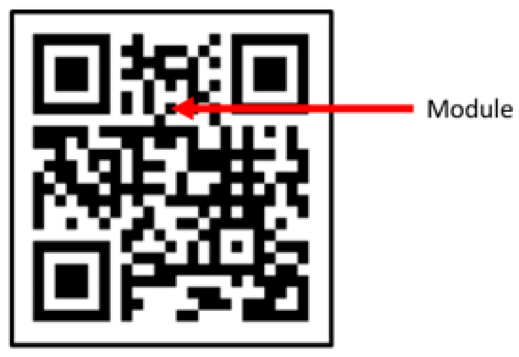
A QR code is a two-dimensional barcode symbol that is categorized as a matrix code. It is made up of black and white squares, known as modules (Figure 1), with the black squares representing a value of 1 and the white squares representing a value of 0.
There are 40 versions of QR codes, with the smallest being Version 1, which consists of 21 × 21 code elements. Each subsequent version increases the number of code elements in the side length by 4. Version 40 has 177 × 177 modules, with a total of 31,329 code elements. The largest numbers of character types, data, and error correction levels are defined separately in each session. The QR code system implements the Reed–Solomon error correction algorithm with four error correction levels. Furthermore, the system divides QR codes into disjoint blocks and performs error correction on each block. Each block consists of codewords, and each codeword contains eight data modules. The higher the error correction level, the lower the storage capacity. The approximate error correction capabilities at each of the four levels are as follows:
- Level L (Low) 7% of codewords can be restored;
- Level M (Medium) 15% of codewords can be restored;
- Level Q (Quartile) 25% of codewords can be restored;
- Level H (High) 30% of codewords can be restored.
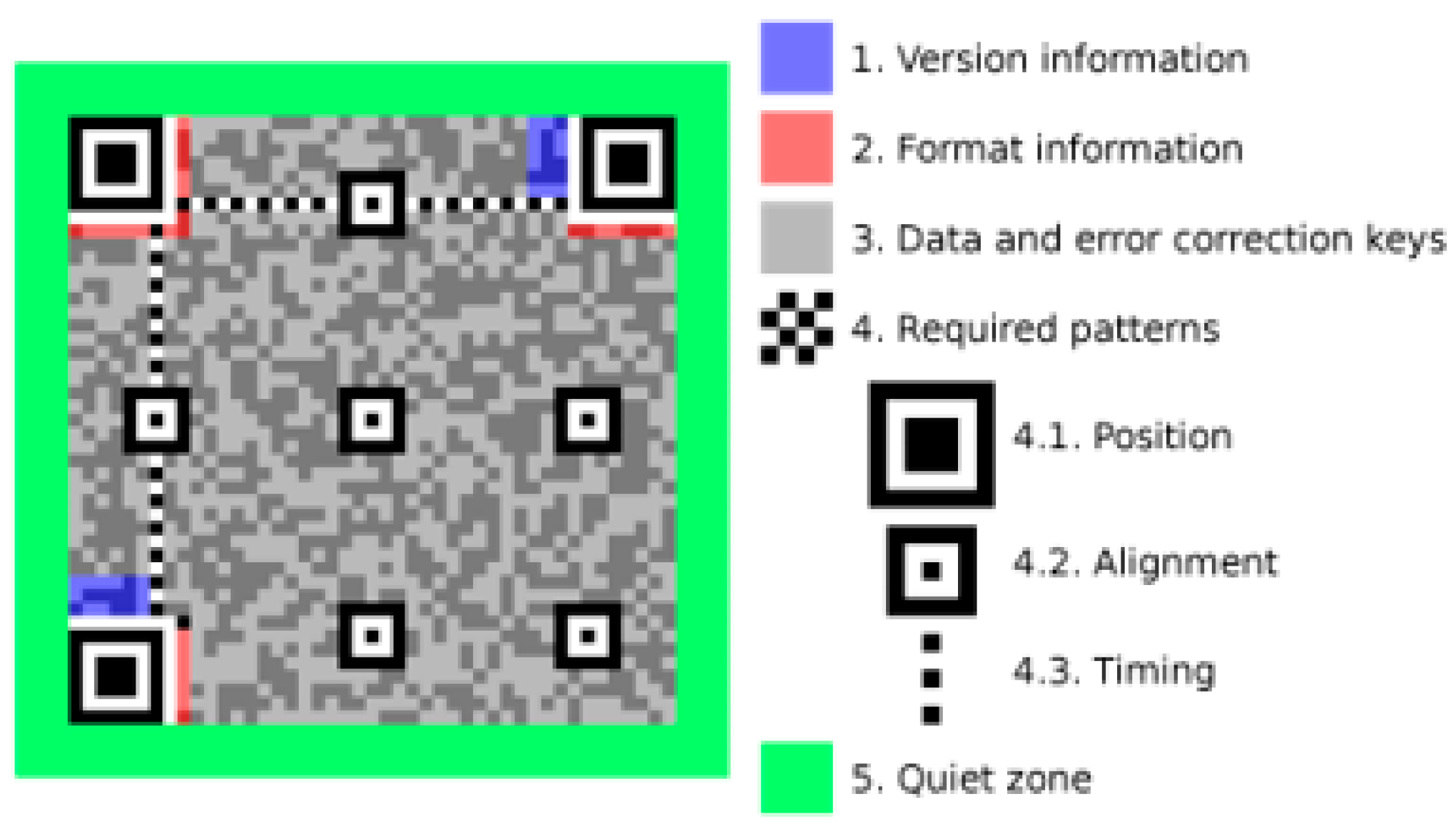
The code elements of a QR code can be divided into non-data areas and data-coding areas. Figure 2 shows the structure of a QR code. The following terms and uses are introduced in the QR code diagram:
2.3.1. Non-Data (Also Known as Functional Patterns)
- The positioning pattern is a crucial feature of the QR code. It consists of three large black-and-white concentric squares located in the upper left and right and lower left. Losing one of these patterns greatly affects recognition, as they are essential for QR code recognition.
- The separator pattern is a continuous white-coded element that surrounds the positioning pattern to distinguish it from other regions.
- The timing pattern is a ribbon of alternating black and white code elements that is barely noticeable as it blends in with the other blocks of codewords. It appears in all versions of QR codes and is also known as the “fixed pattern” due to its fixed alternating pattern and position. The timing pattern consists of two straight lines that confirm the size of the code element.
- The alignment pattern, also known as the alignment marker, is only found in QR code version 1. The other versions require the addition of an alignment pattern for positioning. If the alignment pattern is too large, it can be easily deformed during scanning. However, the alignment pattern can be used as a reference to correct the deformation of the QR code.
2.3.2. Data Codeword Filling Method
In the QR code diagram, the data bytes are arranged in a zig-zag pattern starting from the lower right corner of the matrix and moving upwards in rows of two code elements. When the row reaches the top, the next column of two code elements starts immediately to the left of the previous column and moves downward. If the current column reaches the edge of the matrix, it moves to the next two-code-element column and changes direction. When a function pattern or version format’s reserved area is encountered, the data byte is placed in the next available code element.
The QR code standard specifies codewords as eight binary bits, such as 10,110,010, with a length of 8. Each coded element of the encoded data is first put into a 2 × 4 matrix. In this matrix, the most significant bit of the symbol is represented by 7, and the least significant bit is represented by 0.
2.4. Development of Color QR Code for Visual Beautification
Chu et al. [24] developed halftone QR codes, which improved the quality and appearance of QR codes by replacing each QR code module with smaller, 3 × 3 submodules. The submodules were rearranged through a module subdivision process to create a new, smaller pattern that could be easily manipulated to achieve a desired shape. Garateguy et al. [25] later enhanced this technique by embedding halftone patterns as QR masks into color images. While this technique improved the visibility of the background color, the area of interest in the background image was still covered by a halftone mask, and high-resolution QR codes were needed to minimize readability issues.
Li et al. [26] used image-saliency-detection technology to compute the saliency value of the background image and generate a saliency map, which is an image that highlights the region on which the eye focuses first. This technique, which is based on human perception, allows some areas to be free of QR codewords while maintaining the redundancies of the Reed–Solomon (RS) error-correction blocks. In 2017 and 2018, Lin et al. [27] improved upon this machine-defined saliency map by introducing an interactive framework in which the area of interest could be user-defined by creating strokes on the target area. Another improvement was the implementation of the Adaptive Contrast Enhancement (ACE) [28] algorithm, which enhances image contrast to improve visual quality and increase the number of modules that can be erased with minimal impact on readability.
In 2019, M.-J. Tsai and C.-Y. Hsieh [29] introduced a new method for embedding QR codes. Unlike traditional QR codes, which are embedded in the spatial domain, this method involves storing both the halftone masks and the background image in a discrete wavelet transform (DWT) domain, taking into account the Human Visual System (HVS). This allows the background host image to be considered as part of the scannable region.
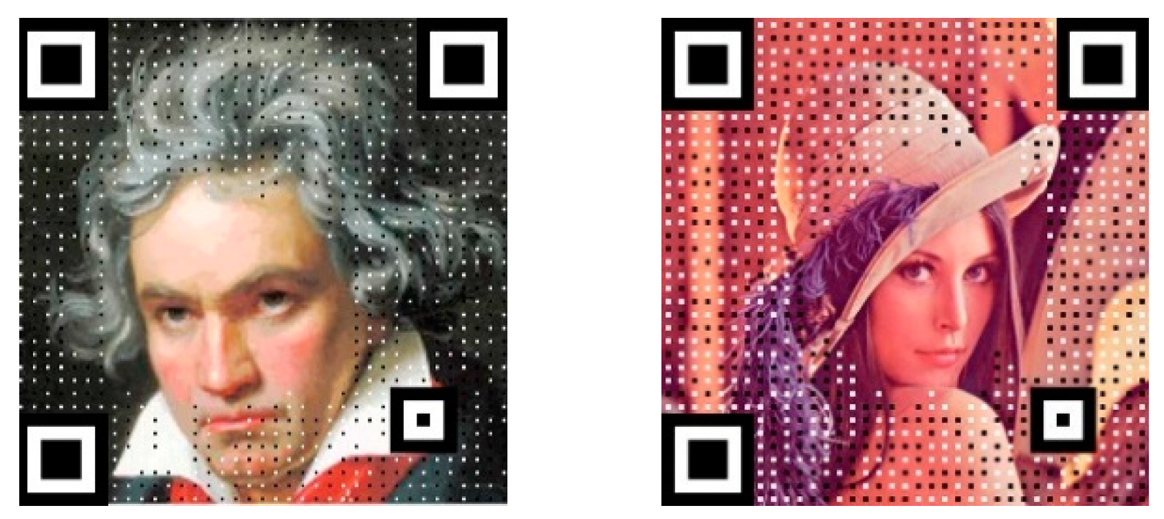
M.-J. Tsai and D.-T. Lin [30] updated the previous work by adding a deep learning solution, Mask R-CNN, which generates an area of interest (Auto Mask) similar to [26], but with the added feature of object detection for the background image. This automated method can expand the area of interest or remove codewords from the furthest area. This latest study on color QR code generation is the primary source for our color QR code dataset. The source images can be seen in Figure 3.
2.5. Convolutional Neural Networks
CNNs have been very effective for classifying complex images since 2012 [20]. LeCun et al. [35] concluded that the reduced number of parameters to be learned is the main benefit of using CNNs, which is better than traditional fully connected neural networks such as SVM. Convolutional layers consist of small kernels that allow the raw image to be used without prior handcrafted feature extraction or data reconstruction. As a result, these layers are extremely effective at extracting high-level features that are fed to fully connected layers. The first convolutional layer transforms the input image into feature maps, while the pooling stage reduces the dimensions of the feature maps, as do other layers. Finally, the last layer is used to classify the input. A CNN is trained using backpropagation and stochastic gradient descent, with the misclassification error driving the weight update of both convolutional and fully connected layers. After training, the output of a network’s layer can be used as a feature vector paired with an external classifier rather than relying solely on the classification of the network layer. The basic structure of a CNN is shown in Figure 4, along with a list of its layers.
- Input layer: This is where the data are fed into the network. The input data, which can be either raw image pixels or their transformations, are fed into the network at the beginning. These data can be selected to better emphasize specific aspects of the image.
- Convolutional layers: These layers contain a series of fixed-size filters used to perform convolution on the image data, generating a so-called feature map. These filters can highlight patterns such as edges and changes in color, which help characterize the image.
- Rectified Linear Unit (ReLU): ReLU layers, which normally follow a convolution operation, apply a non-linear function to the output x of the previous layer, such as f(x) = max(0,x). According to Krizhevsky et al. [20], this function can be computed faster than its equivalents with tanh units in terms of training time with gradient descent. This helps to create rapid convergence in the training process by reducing the vanishing gradient problem and more or less maintaining the constancy of the gradient in all the network layers, thereby speeding up the training process.
- Pooling layers: A pooling layer summarizes the data by applying some linear or non-linear operation, such as generalized mean or max, to the data within a window that slides across the feature maps. This reduces the spatial size of the feature maps used by the subsequent layers and helps the network to focus only on the most important patterns identified by the convolutional layers and ReLU, thereby minimizing computation intensity.
- Fully connected layers: The fully connected layers are located at the end of the network and are used for understanding the patterns generated by the previous layers. They act as classifiers, usually followed by a soft-max layer to determine the class associated with the input image.
- Soft-max layer: The soft-max layer is typically used during training at the network’s end. It normalizes the input values so that they add up to one, and its output can be interpreted as a probability distribution, such as the probability of a sample belonging to each class.
In this deep learning study on identifying QR-code-printed sources, we used pretrained CNN models that have been trained and tested extensively on the ImageNet dataset. These models are useful because their identification performance has already been verified through the ImageNet standard. However, one major drawback of deep learning is that common CNNs typically require thousands or even millions of labeled data for training, which can be unrealistic for many applications due to the time needed to train the model and the lack of available training data.
Some readily available pretrained CNN models, such as AlexNet, GoogleNet, VGG16, ResNet, MobileNetv2, and DenseNet201, are chosen to be tested in this work with BW and color QR codes separately. These QR codes all have nearly identical images that are difficult to distinguish with the human eye unless they are compared side-by-side. This work also represents an alternative approach that meets the above requirements by constructing a simple, lightweight residual model for printed source identification, as discussed in Section 4.
3. Proposed Method
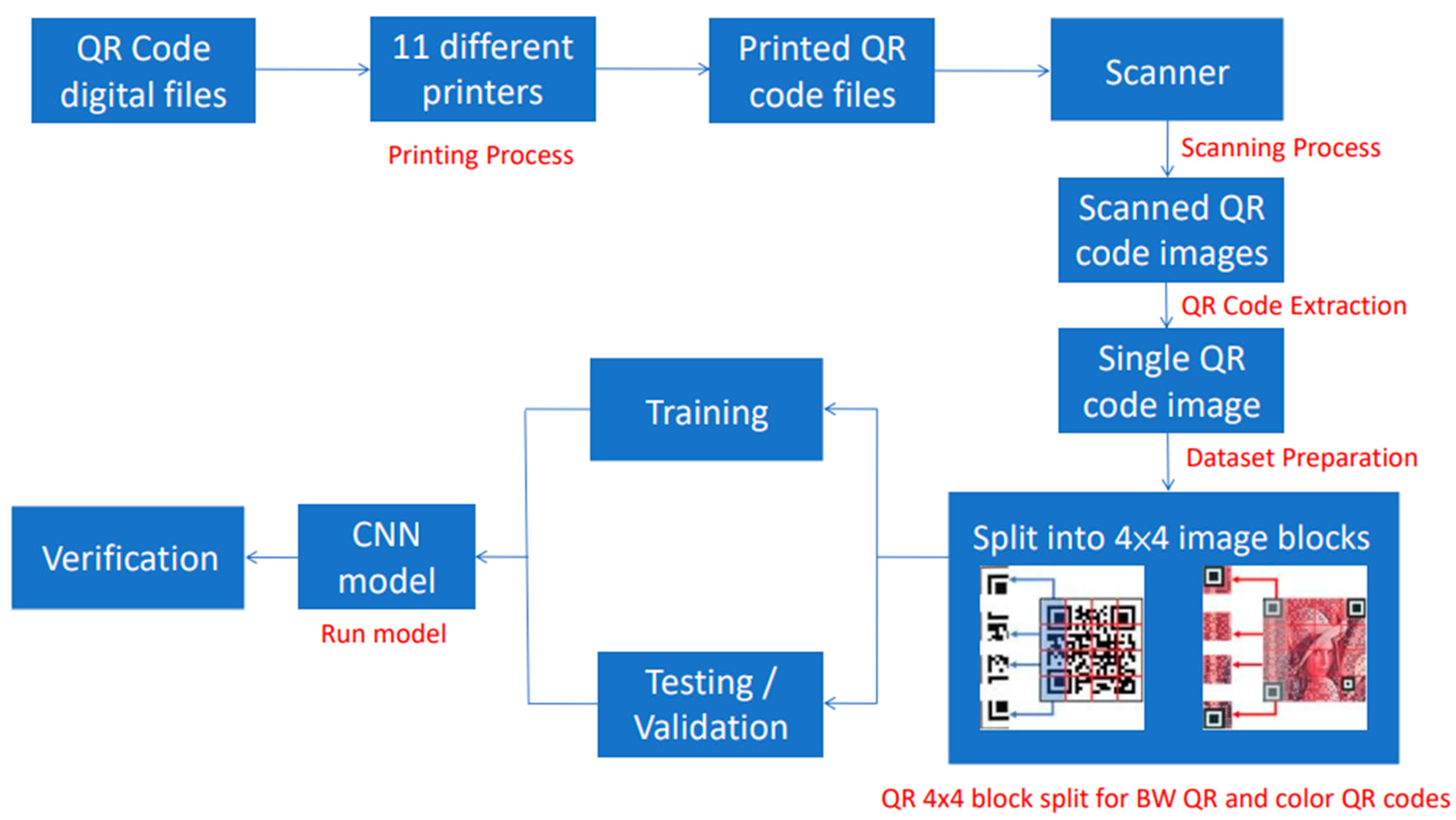
The proposed method is executed based on the supervised deep-learning pipeline for classifying images. There are five steps, starting from the printing process, where the QR code is first generated from digital files. Then, all the QR code documents are arranged to be printed in the same batch. Next, as its name suggests, all the printed QR code documents are scanned in the scanning process, which is also called the digitalization process. QR code extraction is where the scanned documents are thrown into a program, and the QR codes are automatically cropped and saved individually. In dataset preparation, all the cropped QR codes are split into 16 smaller image blocks (Figure 5) before being fed into CNN models during the Run Model process. Only 4 blocks are shown because of limited space (all 16 image blocks are used in the actual training).
The diagram in Figure 5 illustrates the process for the deep learning printed source identification of the QR codes.
- Printing Process:
- Scanning Process: The printed QR codes are digitalized using a dedicated office scanner, and all the documents are saved in TIF lossless image format. BW QR code uses 8-bit grayscale format, while color QR code is saved in 24-bit RGB format.
- QR code extraction: Using MATLAB, the regionprops and imcrop functions are combined to automatically crop and resize all 24 QR codes on one page. This process is looped 24 times from the top left to right.
- Dataset preparation: An open-source image viewer, XnView MP, is implemented to divide all extracted QR codes into 4 × 4 image blocks by batch. Moreover, all BW QR code images are converted from 8-bit format to 24-bit format, as required by the pretrained models. The cropping process does not affect the image quality because the image is neither reconstructed nor resized.
- Run model: The CNN model is operated to put a new set of images into categories.
3.1. Data Collection
To collect the data, a QR code generator is used to produce a link, https://www.iim.nctu.edu.tw/ (10 December 2022), for black and white QR codes, which are saved in a PNG format with a dimension of 512 × 512 pixels.
There are 24 QR code images per page A total of 10 of them are collected for an individual printer model, and 240 QR codes are collected for each printer.
- BW QR codes: 2640 QR codes are collected after printing the documents with 11 individual printers (Table 1).
- Color QR codes: to compare the same model with BW QR codes, documents are printed with 8 printer models, resulting in 1920 color QR codes collected in total.
Those printed pages are then scanned to be digitalized in the TIF format through an Epson Perfection V39 scanner at 400 dpi and saved in an uncompressed form to preserve as many details as possible.
3.2. QR Code Extraction
Through MATLAB, batch-like image extraction is designed specifically for black and white images to cut out all 24 QR code images on the same page by detecting the bounding box individually. There is a rough dimension of 554 × 554 for all the QR codes, although some of them could be bigger or smaller by 1 to 5 pixels based on the printer. Saving all QR code images in the TIF format means that the scanned files are uncompressed images to ensure the intrinsic signatures, such as banding produced by the toner, are still in high resolution.
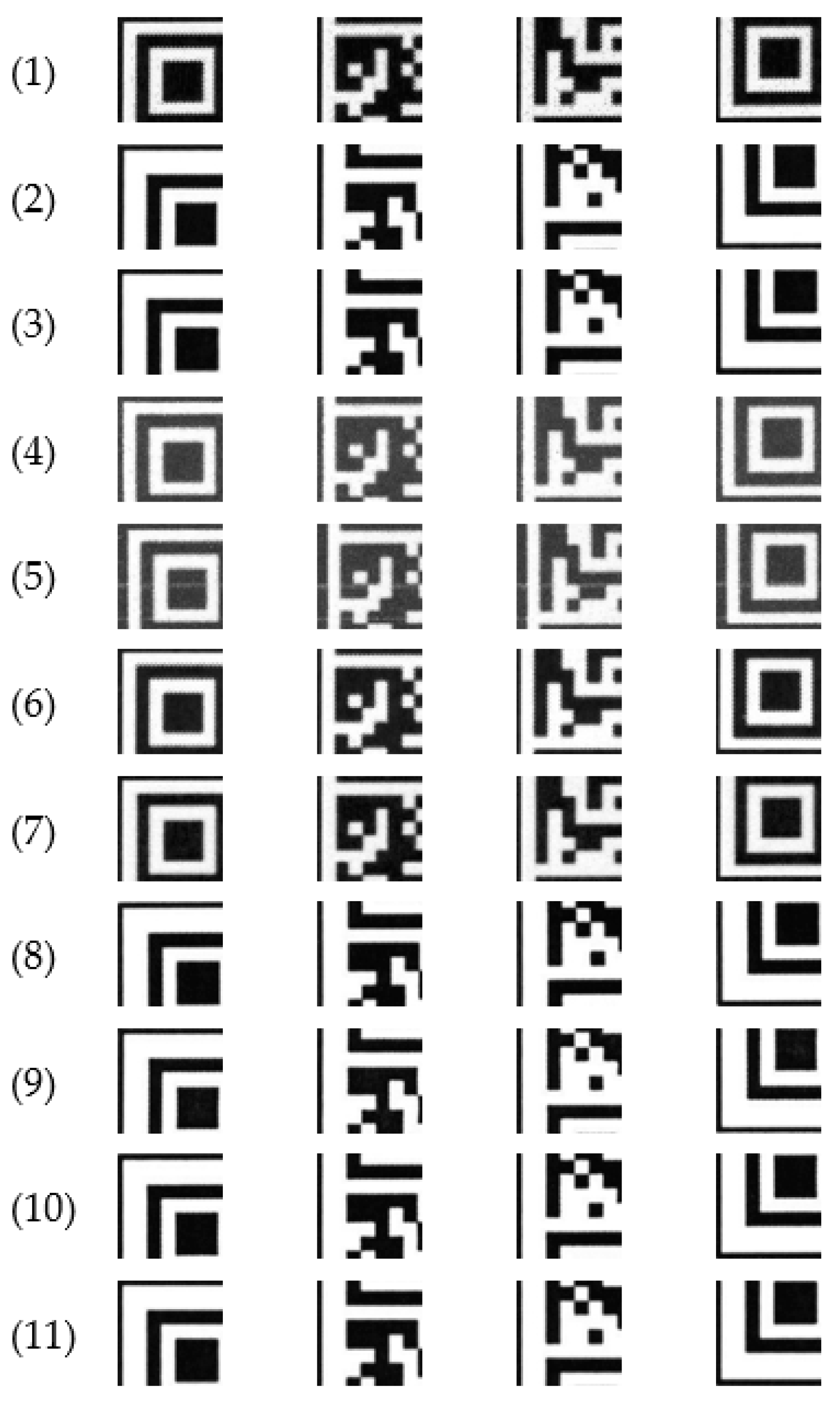
In this step, all the extracted QR codes are divided into 4 × 4-size blocks, as shown in Figure 6 and Figure 7. Consequently, each printer has 240 QR code images, so splitting every image individually into 16 blocks means a total of 240 × 16 = 3840 blocks. Since eleven printers are used for the test, as shown in Table 2, the overall accumulated images become 3840 × 11 = 42,240 blocks.
The QR code images are divided into 4 × 4 blocks, which means 554/4 = ±139 pixels. Since the size of each block of images may be slightly different, they need to be upscaled to a unified dimension. imageDataAugmenter, one of MATLAB’s features is then adapted to upscale and unify all the images to 227 × 227 (AlexNet), 224 × 224 (the rest of the pretrained models), and 160 × 160 (customized model) so that the image blocks can be implemented as input training images. Refer to Figure 6 and Figure 7 for image block illustrations.
In MATLAB, the training and testing/validation sets are divided based on the ratio 80:20 and treated as such. Both of them are combined in every epoch before being averaged into a single identification result.
An image datastore is a device that allows users to store large volumes of image data, even if data are not fitting in memory, and to read batches of images efficiently when processing network training.
Based on the 80:20 ratio, the BW QR Code has a training set of 33,792 images and a test set of 8448 ones. The color QR Code has a training set of 24,576 images and a test set of 6144. The training and test sets are completely separate and use the splitEachLabel function as declared at the beginning of the data preprocessing right after the new images are loaded as an image datastore and waiting to be fed into the network. In MATLAB, the imageDatastore function automatically labels the images based on folder names and stores the data as ImageDatastore objects.
4. Experimental Results
4.1. Training Environment
In terms of the training equipment, tests in the paper are conducted through a PC equipped with AMD Ryzen 7 3700X CPU @3.60 GHz with eight cores, 16 Threads, an NVIDIA GeForce RTX 3090 GPU with 24 GB GDDR6X VRAM, and 32 GB DDR4 2400 MHz RAM with a Windows 10 Education operating system. The source codes of the CNN models are developed in MATLAB.
In this experiment, pre-trained models such as MobileNetv2, VGG16, AlexNet, ResNet, DenseNet201, and GoogleNet have their hyperparameters tweaked, as shown in Table 3.
The only variable in this test is the restricted learning rate. Since all the CNN models were pre-trained at a learning rate of 0.001 on an ImageNet database with over 1 million images and 1000 different categories, the research keeps the learning rate at 0.001 for consistency. Moreover, setting a higher value than recommended, such as 0.01, might result in unstable models with lower validation rates and/or overfitting.
Five image augmentations are used to increase the generalization of the pretrained model during training and to determine whether they could identify each printer’s intrinsic signatures and banding correctly when images are rotated, mirrored, and scaled. These augmentations are Xreflection, Xtranslation, Ytranslation, Xscale, and Yscale. The augmentation techniques applied to the training dataset are summarized in Table 4.
4.2. Performance Evaluation of BW QR Codes
To evaluate the fine-tuned pretrained models, standard performance metrics are used, including precision and accuracy, recall (or sensitivity), and specificity for each optimizer. These metrics are implemented to determine the best parts in terms of prediction accuracy, overall stability, and training duration, as shown in Table 5.
For identifying the BW QR code printed source, ResNet50 SGDM took first place, with 100% accuracy, based on perfect scores for all three performance metrics. In second place, ResNet18 had a training time almost 50% faster than ResNet50 SGDM, with minimal loss in prediction accuracy, precision, and recall. MobileNetv2 took third place at 99.7%, with a training time of almost 117 min, or about 9 min longer than ResNet50. The results of our customized model are also included for comparison.
The results for identifying each printer model’s intrinsic signatures are shown at the bottom of Table 6, with the accuracy for each printer being measured to determine which printer model is the easiest and hardest to distinguish for each CNN model.
According to the results in Table 6, the printer that can be most easily identified using the pretrained CNN models is the Epson L3110 (printer model number 5). Please refer to Table 1 for the Model Name. It is worth noting that this printer has the most prominent banding compared to the other models. The Fuji Xerox P355d (printer model number 6) takes the second position, while the third position is a tie between the HP M283 (multicolor laserjet printer that can also print in color) and the HP M401 (black-and-white laserjet printer). The M283 has a deeper and more consistent black color with smooth color transitions, while the M401 has a less consistent black color with some white patches visible upon closer examination.
Model number 11, the Konica Minolta Bizhub C364, has a 90% identification rate. It is vital to think that this does not necessarily mean that it is the most difficult printer to identify. In fact, a 90% identification rate is still quite impressive. The main reason for this model’s lower average identification rate is that GoogleNet achieved significantly lower accuracy when using both Adam and RMSprop optimization algorithms.
Performance Evaluation for Color QR Codes
In general, pretrained CNN models tend to train faster when using a Color QR Code dataset rather than a BW QR Code dataset.
While it might be expected that an 8-bit grayscale image would be easier to process due to having fewer color channels than a 24-bit RGB image, it turns out that more features can be extracted from a 24-bit image, which significantly speeds up the inference process of the CNN models in this case.
According to Table 7, MobileNetv2 with the RMSprop optimization algorithm has the highest accuracy, at 99.9%, after 103 min of training. VGG16 comes in second place, with an accuracy of 99.8% and a faster training time of 86 min. AlexNet takes third place, with a training time of only 33 min and an accuracy of 99.6%. AlexNet has the fastest training time of all the models and is also one of the top three for accuracy, beating ResNet18 by almost 10 min. Previously, ResNet18 was known for having the fastest training time in a BW QR code experiment.
Table 8 shows the results of the per-printer identification. The same indicators are used to evaluate the accuracy of each printer and optimization algorithm in order to determine the best-performing CNN model.
Model number 2, the Canon LBP9200C, is the easiest printer to identify. In second place is model number 4, the Fuji Xerox DocuCentre-IV, with 98.6% identification accuracy. Model number 1, the Canon imageRunner 6555i, takes third place with 97.7% accuracy, just 0.9% behind the second-place printer.
4.3. Customized Fine-Tuned Residual Model Structure
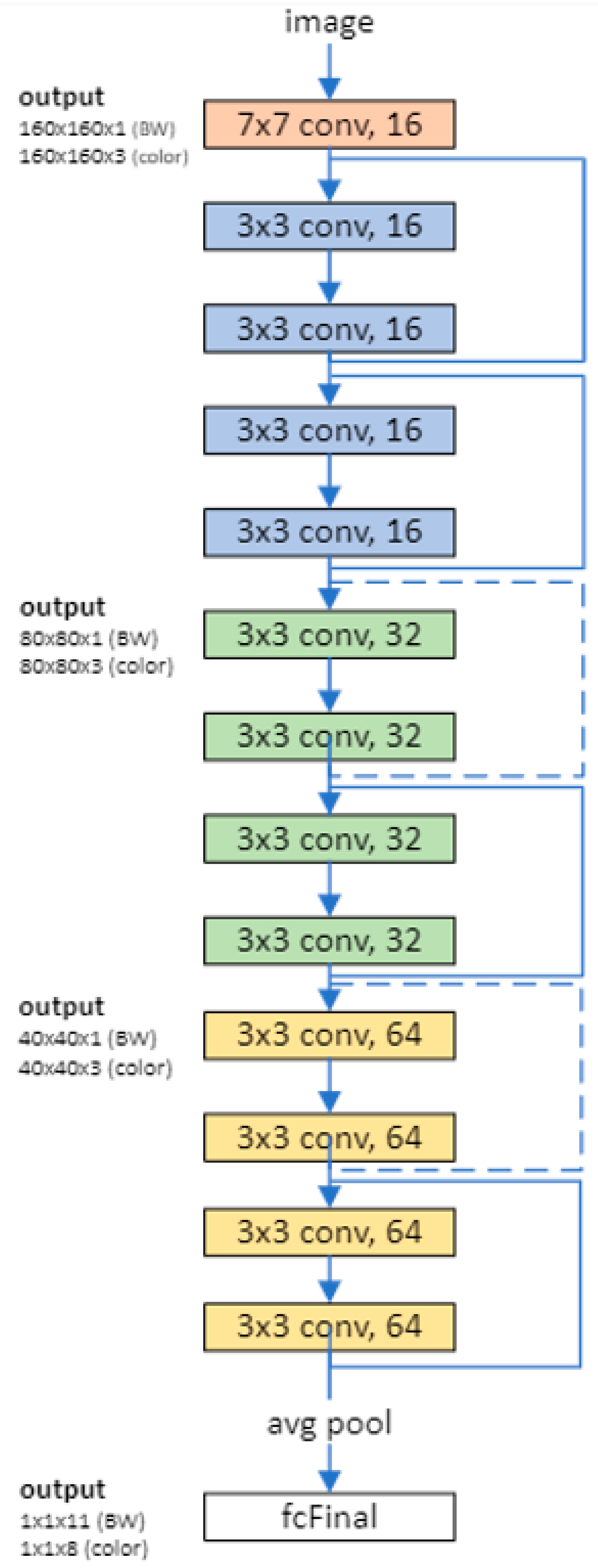
In this study, a deep learning neural network with residual connections is proposed (as shown in Figure 8) and trained on both BW and color QR code image blocks. Residual connections are a common feature of convolutional neural network architecture because they can improve the gradient flow through the network and enable the training of deeper networks.
For many applications, a network that consists of a simple sequence of layers is sufficient. However, some applications require networks with a more complex graph structure, in which inputs come from multiple layers and outputs go to multiple layers. These types of networks are often referred to as directed acyclic graph (DAG) networks.
A residual network is a type of DAG network that includes residual (or shortcut) connections that bypass the main layers of the network. These residual connections allow the parameter gradients to more easily propagate from the output layer of the network to the earlier ones and result in deeper training, which improves accuracy for challenging tasks, such as identifying intrinsic signatures, which often look identical in most datasets. The overall structure of our residual model is shown in Figure 8, and its architecture is detailed in Table 9.
4.3.1. Defining the Network Architecture: The Components of the Residual Network Architecture
- The key branch of the network is divided into various twisting layers with batch normalization and ReLU activation functions that are connected consecutively.
- The network has residual connections that bypass the convolutional units in the main branch. An element adds the outputs of the residual connections and convolutional units. The residual connections must also include 1-by-1 convolutional layers when the activation size differs. In addition, they will allow the parameter gradients to more easily propagate from the output layer to the earlier layers of the network, enabling training networks.
4.3.2. Creating the Main Branch of the Network with Five Sections
- The network begins with an initial section that includes the image input layer and an initial convolution with activation.
- The network has three stages of convolutional layers with different feature sizes (160-by-160, 80-by-80, and 40-by-40) and different kernel sizes (7 × 7, 5 × 5, and 3 × 3) in the first convolution layer. Each stage includes N convolutional units. In this example, N = 2. Each convolutional unit contains two 3-by-3 convolutional layers with activations. The net width parameter shows the network defined as the number of filters in the convolutional layers in the first stage of the network. The first convolutional units in the second and third stages down-sample the spatial dimensions by a factor of two. The number of filters is accumulated by a factor of two each time spatial down-sampling is performed in order to maintain approximately the same amount of computation in each individual convolutional layer throughout the network.
- The final section of the network includes global average pooling, fully connected, softmax, and classification layers.
4.4. Performance Evaluation of Customized Fine-Tuned Residual Model
The customized model’s optimizers (SGDM, Adam, and RMSprop) and hyperparameters (as detailed in Table 4) are also used to train and evaluate the model’s performance. Table 10 shows the accuracy for different optimizers and kernel sizes. The model performs best with an SGDM optimizer for BW QR codes and an Adam optimizer for color QR codes. It was also found that the model works best with a kernel size of 7 × 7. Therefore, a kernel size of 7 × 7 is used to evaluate the standard performance metrics in the next evaluation.
Table 11 displays the standard performance metrics, including accuracy, precision, recall (or sensitivity), and specificity, for each optimizer for BW QR codes (A) and color QR codes (B).
As shown in Table 11, the training of BW QR codes is still slower than the training of color QR codes, similar to the results of the previous experiment comparing pretrained CNN models. However, the training time for our model for BW and color QR codes only differs by about 9–12 min, which is similar to the training time for the pretrained ResNet18 model in the earlier experiment for the BW QR Code.
Our model also has better overall stability in terms of accuracy across the three provided optimizers. For the BW QR code results in Table 5 SGDM has the fastest training time at 51.3 min, about 4 min faster than the other two optimizers. Adam and RMSprop provide better identification accuracy (99.8%) but at the cost of longer training times.
For identifying a color QR code, RMSprop has fluctuating accuracy between 98% and 99%, making SGDM and Adam the better choices. Table 10B shows that SGDM has the fastest training time for color QR codes at 40.3 min. However, the performance of SGDM and Adam is consistently very similar at 99.7%.
5. Conclusions and Future Work
5.1. Conclusions
To address the issue of QR codes being easily reproducible during the printing process, we used a printed source identification method based on BW and color QR codes that were trained under a customized residual network CNN model in this experiment. This method was found to be as efficient as fine-tuned pretrained CNN models. In general, dividing QR code images into 16 blocks significantly improved the identification accuracy and consistency among the different pretrained CNN models.
It is interesting to note that each pretrained CNN model behaves differently when identifying the printed source of BW and color QR codes. While ResNet performs well for BW QR codes, it lags behind MobileNetv2 and the more linear models such as AlexNet and VGG16 (using SGDM optimization) for color QR codes, despite the latter generally having more intrinsic features.
Our simplified residual model is suitable for popular printer models that are commonly used in offices and local convenience stores. Its relatively short training time, high accuracy, and adjustable hyperparameters make it effective at generalizing datasets from an intrinsic signature perspective and at detecting the intrinsic signatures of QR code datasets.
5.2. Future Works
Now that the printed source identification of scanned QR code images can achieve high classification results using deep learning models, we believe it is time to tackle more challenging tasks. These could include adding upsampled images (using Nearest Neighbor, Bilinear, Bicubic, etc.) to the test/validation set to assess their impact on identification accuracy, adding a Gaussian blur attack to the QR code and analyzing the noise pattern, and printing the images on different types of paper to study the effects of surface texture on image clarity. Additionally, a reverse engineering approach could be used to identify the extent of wear and tear on mechanical components by examining intrinsic features and banding at various levels of degradation.
Author Contributions
Conceptualization, M.-J.T. and T.-M.C.; methodology, M.-J.T.; software, T.-M.C..; validation, M.-J.T., Y.-C.L. and T.-M.C.; formal analysis, M.-J.T.; investigation, T.-M.C.; resources, Y.-C.L.; data curation, M.-J.T.; writing—original draft preparation, M.-J.T.; writing—review and editing, Y.-C.L.; visualization, T.-M.C.; supervision, M.-J.T.; project administration, Y.-C.L.; All authors have read and agreed to the published version of the manuscript.
Funding
The National Science Council partially supported this work in Taiwan, Republic of China, under MOST 109-2410-H-009-022-MY3.
Institutional Review Board Statement
Not applicable.
Informed Consent Statement
Patient consent was waived because no human beings were involved in the research.
Data Availability Statement
All data are publicly available.
Acknowledgments
The authors thank the National Center for High-performance Computing (NCHC) of National Applied Research Laboratories (NARLabs) in Taiwan for the provision of computational and storage resources.
Conflicts of Interest
The authors declare no conflict of interest.
References
- Zhu, B.; Wu, J.; Kankanhalli, M.S. Print signatures for document authentication. In Proceedings of the 10th ACM Conference on Computer and Communications Security (CCS), Washington, DC, USA, 27–30 October 2003; pp. 145–154. [Google Scholar]
- Chiang, P.J.; Khanna, N.; Mikkilineni, A.K.; Segovia, M.V.O.; Suh, S.; Allebach, J.P.; Chiu, G.T.-C.; Delp, E.J. Printer and scanner forensics. IEEE Signal Process. Mag. 2009, 26, 72–83. [Google Scholar] [CrossRef]
- Cicconi, F.; Lazic, V.; Palucci, A.; Assis, A.C.A.; Saverio Romolo, F. Forensic analysis of Commercial Inks by Laser-Induced Breakdown Spectroscopy (LIBS). Sensors 2020, 20, 3744. [Google Scholar] [CrossRef] [PubMed]
- ABraz; Lopez-Lopez, M.; Garcia-Ruiz, C. Raman spectroscopy for forensic analysis of inks in questioned documents. Forensic Sci. Int. 2013, 232, 206–212. [Google Scholar]
- Gal, L.; Belovicova, M.; Oravec, M.; Palkova, M.; Ceppan, M. Analysis of laser and inkjet prints using spectroscopic methods for forensic identification of questioned documents. Symp. Graph. Arts 1993, 10, 1–8. [Google Scholar]
- Chu, P.-C.; Cai, B.; Tsoi, Y.; Yuen, R.; Leung, K.; Cheung, N.-H. Forensic analysis of laser printed ink by x-ray fluorescence and laser-excited plume fluorescence. Anal. Chem. 2013, 85, 4311–4315. [Google Scholar] [CrossRef]
- Barni, M.; Podilchuk, C.I.; Bartolini, F.; Delp, E.J. Watermark embedding: Hiding a signal within a cover image. IEEE Commun. Mag. 2001, 39, 102–108. [Google Scholar] [CrossRef]
- Fu, M.S.; Au, O. Data hiding in halftone images by stochastic error diffusion. In Proceedings of the IEEE International Conference Acoustics, Speech, and Signal Processing, 2001, (ICASSP 01), Salt Lake City, UT, USA, 7–11 May 2001; Volume 3, pp. 1965–1968. [Google Scholar]
- Bulan, O.; Monga, V.; Sharma, G.; Oztan, B. Data embedding in hardcopy images via halftone-dot orientation modulation. In Proceedings of the Security, Forensics, Steganography, and Watermarking of Multimedia Contents X, San Jose, CA, USA, 27–31 January 2008; Volume 6819, p. 68190C-1-12. [Google Scholar]
- Kim, D.-G.; Lee, H.-K. Colour laser printer identification using halftone texture fingerprint. Electron. Lett. 2015, 51, 981–983. [Google Scholar] [CrossRef]
- Ferreira, A.; Bondi, L.; Baroffio, L.; Bestagini, P.; Huang, J.; Dos Santos, J.A.; Tubaro, S.; Rocha, A.D.R. Data-driven feature characterization techniques for laser printer attribution. IEEE Trans. Inf. Forensics Secur. 2017, 12, 1860–1872. [Google Scholar] [CrossRef]
- Mikkilineni, A.K.; Chiang, P.-J.; Ali, G.N.; Chiu, G.T.-C.; Allebach, J.P.; Delp, E.J. Printer identification based on textural features. In Proceedings of the International Conference on Digitial Printing Technologies, West Lafayette, IN, USA, 18–23 October 2004; pp. 306–311. [Google Scholar]
- Mikkilineni, A.K.; Arslan, O.; Chiang, P.J.; Kumontoy, R.M.; Allebach, J.P.; Chiu, G.T.; Delp, E.J. Printer forensics using SVM techniques. In Proceedings of the International Conference on Digitial Printing Technologies, Baltimore, MD, USA, 18–23 September 2005; pp. 223–226. [Google Scholar]
- Mikkilineni, K.A.; Chiang, P.-J.; Ali, G.N.; Chiu, G.T.C.; Allebach, J.P.; Delp, E.J. Printer identification based on graylevel co-occurrence features for security and forensic applications. In Proceedings of the SPIE International Conference on Security, Steganography, and Watermarking of Multimedia Contents VII, San Jose, CA, USA, 17–20 January 2005; Volume 5681, pp. 430–441. [Google Scholar]
- Ferreira, A.; Navarro, L.C.; Pinheiro, G.; dos Santos, J.A.; Rocha, A. Laser printer attribution: Exploring new features and beyond. Forensic Sci. Int. 2015, 247, 105–125. [Google Scholar] [CrossRef]
- Tsai, M.-J.; Yuadi, I.; Tao, Y.-H. Decision-theoretic model to identify printed sources. Multimed. Tools Appl. 2018, 77, 27543–27587. [Google Scholar] [CrossRef]
- Joshi, S.; Khanna, N. Single classifier-based passive system for source printer classification using local texture features. IEEE Trans. Inf. Forensics Secur. 2018, 13, 1603–1614. [Google Scholar] [CrossRef] [Green Version]
- Tsai, M.-J.; Yin, J.-S.; Yuadi, I.; Liu, J. Digital forensics of printed source identification for Chinese characters. Multimed. Tools Appl. 2014, 73, 2129–2155. [Google Scholar] [CrossRef]
- LeCunn, Y.; Bengio, Y.; Hinton, G. Deep learning. Nature 2015, 521, 436–444. [Google Scholar] [CrossRef] [PubMed]
- Krizhevsky, A.; Sutskever, I.; Hinton, G.E. ImageNet classification with deep convolutional neural networks. Commun. ACM 2017, 60, 84–90. [Google Scholar] [CrossRef] [Green Version]
- Kim, D.-G.; Hou, J.-U.; Lee, H.-K. Learning deep features for source color laser printer identification based on cascaded learning. Neurocomputing 2019, 365, 219–228. [Google Scholar] [CrossRef] [Green Version]
- Guo, Z.-Y.; Zheng, H.; You, C.-H.; Xu, X.-H.; Wu, X.-B.; Zheng, Z.-H.; Ju, J.-P. Digital forensics of scanned QR code images for printer source identification using bottleneck residual block. Sensors 2020, 20, 6305. [Google Scholar] [CrossRef]
- QR Code. Available online: https://en.wikipedia.org/wiki/QR_code#/media/File:QR_Code_Structure_Example_3.svg (accessed on 6 January 2022).
- Chu, H.-K.; Chang, C.-S.; Lee, R.-R.; Mitra, N.J. Halftone QR codes. ACM Trans. Graph. 2013, 32, 217. [Google Scholar] [CrossRef]
- Garateguy, G.J.; Arce, G.R.; Lau, D.L.; Villarreal, O.P. QR Images: Optimized Image Embedding in QR Codes. IEEE Trans. Image Process. 2014, 23, 2842–2853. [Google Scholar] [CrossRef]
- Li, L.; Qiu, J.; Lu, J.; Chang, C.-C. An aesthetic QR code solution based on error correction mechanism. J. Syst. Softw. 2016, 116, 85–94. [Google Scholar] [CrossRef]
- Lin, L.; Wu, S.; Liu, S.; Jiang, B. Interactive QR code beautification with full background image embedding. In Proceedings of the SPIE International Conference on Second International Workshop on Pattern Recognition, Singapore, 1–3 May 2017; Volume 10443, p. 1044317. [Google Scholar]
- Lin, L.; Zou, X.; He, L.; Liu, S.; Jiang, B. Aesthetic QR code generation with background contrast enhancement and user interaction. In Proceedings of the SPIE International Conference on Third International Workshop on Pattern Recognition, Jinan, China, 26–28 May 2018; p. 108280G. [Google Scholar]
- Tsai, M.-J.; Hsieh, C.-Y. The visual color QR code algorithm (DWT-QR) based on wavelet transform and human vision system. Multimed. Tools Appl. 2019, 78, 21423–21454. [Google Scholar] [CrossRef]
- Tsai, M.-J.; Lin, D.-T. QR Code Beautification by Deep Learning Technology. Master’s Thesis, National Yang Ming Chiao Tung University, Hsinchu, Taiwan, 2021. [Google Scholar]
- Do, T.-N. Incremental and parallel proximal SVM algorithm tailored on the Jetson Nano for the ImageNet challenge. Int. J. Web Inf. Syst. 2022, 18, 137–155. [Google Scholar] [CrossRef]
- Tsai, M.-J.; Peng, S.-L. QR code beautification by instance segmentation (IS-QR). Digit. Signal Process. 2022, 133, 103887. [Google Scholar] [CrossRef]
- Wang, Z.; Zuo, C. Zeng. SAE based unified double JPEG compression detection system for Web image forensics. Int. J. Web Inf. Syst. 2021, 17, 84–98. [Google Scholar] [CrossRef]
- Tsai, M.-J.; Wu, H.-U.; Lin, D.T. Auto ROI & mask R-CNN model for QR code beautification (ARM-QR). Multimed. Syst. 2023. [Google Scholar] [CrossRef]
- Lecun, Y.; Bottou, L.; Bengio, Y.; Haffner, P. Gradient-based learning applied to document recognition. Proc. IEEE 1998, 86, 2278–2324. [Google Scholar] [CrossRef] [Green Version]
- Transfer Learning in Keras Using VGG16. 2020. Available online: https://thebinarynotes.com/transfer-learning-keras-vgg16/ (accessed on 7 February 2022).
Figure 1.
QR code basic unit diagram.

Figure 2.
QR code (version 7) structure [23].
Figure 2.
QR code (version 7) structure [23].

Figure 3.
Sample QR Codes generated from [30].
Figure 3.
Sample QR Codes generated from [30].

Figure 4.
General modern CNN architecture [36].
Figure 4.
General modern CNN architecture [36].

Figure 5.
Proposed method’s process flowchart.

Figure 6.
Image samples for BW QR codes printed by 11 printers (please note that each number refers an item in Table 1 for the printer and brand model).
Figure 6.
Image samples for BW QR codes printed by 11 printers (please note that each number refers an item in Table 1 for the printer and brand model).

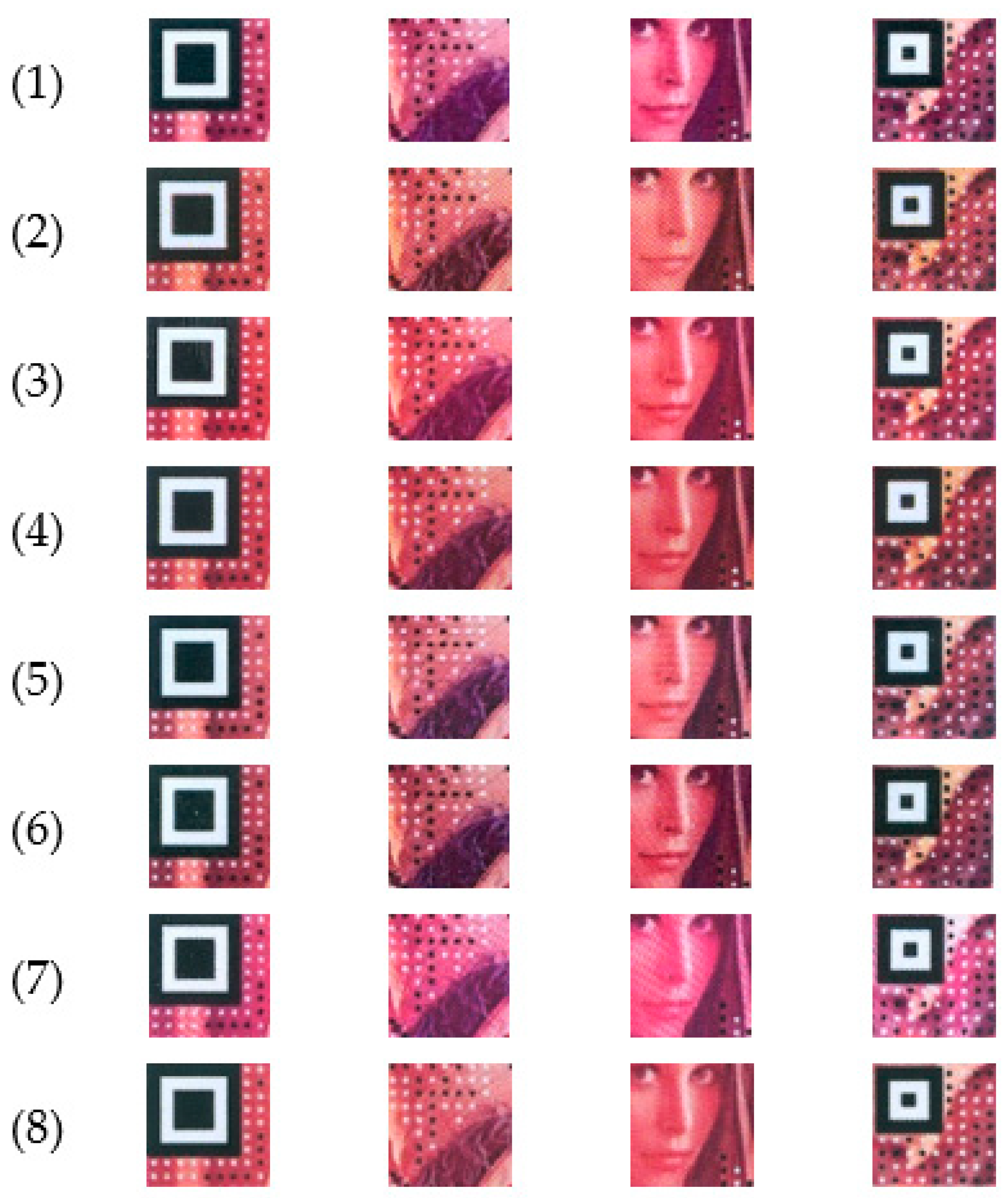
Figure 7.
Image samples for color QR codes (see Table 2 for printer brands).
Figure 7.
Image samples for color QR codes (see Table 2 for printer brands).

Figure 8.
Network architecture of the customized residual network. The dotted shortcuts increase dimensions. Kernel input of the first layer can be modified into [7 × 7], [5 × 5], or [3 × 3]. Refer to Table 9 for the residual model’s architecture.
Figure 8.
Network architecture of the customized residual network. The dotted shortcuts increase dimensions. Kernel input of the first layer can be modified into [7 × 7], [5 × 5], or [3 × 3]. Refer to Table 9 for the residual model’s architecture.


Table 1.
Printer and Brand Model List (BW QR Code).
| No | Brand | Model |
|---|---|---|
| 1 | Canon | LBP3310 |
| 2 | Canon | LBP6300 |
| 3 | Canon | M417 LIPSX |
| 4 | Epson | L350 |
| 5 | Epson | L3110 |
| 6 | Fuji Xerox | P355d |
| 7 | HP | M283 |
| 8 | HP | M377 |
| 9 | HP | M401 |
| 10 | HP | M425 |
| 11 | Konica Minolta | Bizhub C364 |
Table 2.
Printer Brand and Model List (Color QR Code).
| No | Brand | Model |
|---|---|---|
| 1 | Canon | ImageRunner 6555i |
| 2 | Canon | LBP9200C |
| 3 | Fuji Xerox | ApeosPort-VII |
| 4 | Fuji Xerox | DocuCentre-IV |
| 5 | HP | M283 |
| 6 | HP | M377 |
| 7 | Konica Minolta | Magicolor 1690 |
| 8 | Kyocera | Ecosys M5520 |
Table 3.
HyperParameters for All CNN Models.
| Parameter | Value/Type |
|---|---|
| Image Size | 160 × 160, 224 × 224, 227 × 227 |
| Cross Validation | Holdout |
| Training/Testing | 80/20 |
| Optimizer | SGDM, ADAM, RMSprop |
| Max Epochs | 30 |
| Minibatch Size | 64 |
| Shuffle | Every epoch |
| Initial Learn Rate | 10−3 no decay |
Table 4.
Image Augmentation Parameters.
| Augmentation Type | Purpose | Value |
|---|---|---|
| RandXReflection | Reflection in the left-right direction randomly appears, specified as a logical scalar. The image is reflected horizontally with a 50% probability | 1 (true) |
| RandXTranslation | Moving the image in the X or Y direction (or both) from the center coordinate. This forces the convolutional neural network to look everywhere within the image dimension. | [−30, 30] |
| RandYTranslation | ||
| RandXScale | The image is scaled outward or inward. While scaling outward, the final image size is larger than the original. Most image frameworks cut out a section from the new image, with a size equal to the original image. Scaling inward reduces the image size, forcing the model to make assumptions about what lies beyond the boundary. | [0.9, 1.1] |
| RandYScale |
Table 5.
Performance Metrics for BW QR Code.
| Model Name | Optimizer | Accuracy (%) | Precision | Recall | Specificity | Train Time (min) |
|---|---|---|---|---|---|---|
| AlexNet | SGDM | 97.7 | 0.98 | 0.98 | 0.99 | 143 |
| Adam | 9.09 | 0.01 | 0.09 | 0.91 | -- | |
| RMSprop | 9.09 | 0.01 | 0.09 | 0.91 | -- | |
| GoogleNet | SGDM | 98.3 | 0.98 | 0.98 | 0.99 | 65 |
| Adam | 89.8 | 0.94 | 0.90 | 0.99 | 68 | |
| RMSprop | 84.2 | 0.86 | 0.84 | 0.98 | 66 | |
| DenseNet201 | SGDM | 99.7 | 0.99 | 0.99 | 1.00 | 839 |
| Adam | 97.8 | 0.98 | 0.98 | 0.99 | 1090 | |
| RMSprop | 97.8 | 0.98 | 0.98 | 0.99 | 984 | |
| MobileNetv2 | SGDM | 99.7 | 0.99 | 0.99 | 0.99 | 117 |
| Adam | 99.3 | 0.99 | 0.99 | 0.99 | 151 | |
| RMSprop | 99.7 | 0.99 | 0.99 | 1.00 | 136 | |
| ResNet18 | SGDM | 99.9 | 0.99 | 0.99 | 1.00 | 53 |
| Adam | 99.4 | 0.99 | 0.99 | 0.99 | 55 | |
| RMSprop | 99.4 | 0.99 | 0.99 | 0.99 | 49 | |
| ResNet50 | SGDM | 99.9 | 1.00 | 1.00 | 1.00 | 108 |
| Adam | 99.5 | 0.99 | 0.99 | 0.99 | 124 | |
| RMSprop | 99.5 | 0.99 | 0.99 | 0.99 | 121 | |
| VGG16 | SGDM | 99.6 | 0.99 | 0.99 | 1.00 | 114 |
| Adam | 9.09 | 0.01 | 0.09 | 0.91 | -- | |
| RMSprop | 9.09 | 0.01 | 0.09 | 0.91 | -- | |
| Our Model | SGDM | 99.7 | 0.99 | 0.99 | 1.00 | 51 |
| Adam | 99.7 | 0.99 | 0.99 | 1.00 | 59 | |
| RMSprop | 99.8 | 0.99 | 0.99 | 1.00 | 55 |
(“--” means data can be ignored).
Table 6.
BW QR Code Per Printer Identification Result for Each Pretrained CNN Model.
| Model Name | Optimizer | Accuracy | 1 | 2 | 3 | 4 | 5 | 6 | 7 | 8 | 9 | 10 | 11 |
|---|---|---|---|---|---|---|---|---|---|---|---|---|---|
| Alex Net | SGDM | 0.9770 | 0.882 | 1 | 1 | 1 | 1 | 0.973 | 0.991 | 1 | 0.995 | 0.987 | 0.921 |
| Adam | 0.9090 | -- | -- | -- | -- | -- | -- | -- | -- | -- | -- | -- | |
| RMSprop | 0.9090 | -- | -- | -- | -- | -- | -- | -- | -- | -- | -- | -- | |
| Google Net | SGDM | 0.9828 | 0.986 | 1 | 1 | 1 | 0.997 | 1 | 0.995 | 0.978 | 1 | 0.910 | 0.945 |
| Adam | 0.8981 | 0.936 | 0.943 | 1 | 1 | 1 | 1 | 0.997 | 0.992 | 0.995 | 0.829 | 0.186 | |
| RMSprop | 0.8420 | 0.984 | 0.913 | 0.839 | 0.785 | 1 | 1 | 0.913 | 0.855 | 0.931 | 0.727 | 0.315 | |
| Dense Net201 | SGDM | 0.9969 | 1 | 1 | 1 | 0.999 | 1 | 1 | 1 | 0.992 | 1 | 0.975 | 1 |
| Adam | 0.9776 | 0.954 | 0.984 | 1 | 1 | 1 | 1 | 0.990 | 0.842 | 0.996 | 1 | 0.987 | |
| RMSprop | 0.9776 | 0.958 | 0.997 | 1 | 1 | 1 | 1 | 1 | 0.801 | 0.997 | 1 | 1 | |
| Mobile Netv2 | SGDM | 0.9978 | 1 | 1 | 1 | 1 | 1 | 0.995 | 0.995 | 0.997 | 1 | 0.999 | 0.990 |
| Adam | 0.9928 | 0.930 | 1 | 1 | 1 | 1 | 1 | 1 | 0.997 | 0.995 | 0.999 | 1 | |
| RMSprop | 0.9966 | 0.999 | 1 | 1 | 1 | 1 | 1 | 1 | 1 | 0.964 | 1 | 1 | |
| Res Net18 | SGDM | 0.9987 | 0.995 | 1 | 1 | 1 | 1 | 1 | 0.997 | 0.999 | 1 | 0.997 | 0.997 |
| Adam | 0.9943 | 1 | 0.999 | 0.969 | 1 | 1 | 0.995 | 0.987 | 0.993 | 0.996 | 1 | 0.999 | |
| RMSprop | 0.9944 | 0.986 | 1 | 0.999 | 1 | 1 | 0.987 | 0.996 | 0.995 | 0.987 | 0.990 | 1 | |
| Res Net50 | SGDM | 0.9996 | 1 | 1 | 1 | 1 | 1 | 1 | 1 | 1 | 1 | 1 | 0.996 |
| Adam | 0.9947 | 0.996 | 1 | 0.993 | 1 | 1 | 0.974 | 0.996 | 0.995 | 0.992 | 0.999 | 0.996 | |
| RMSprop | 0.9946 | 0.987 | 0.999 | 0.995 | 1 | 1 | 0.986 | 0.993 | 0.995 | 0.993 | 0.996 | 0.996 | |
| VGG 16 | SGDM | 0.9960 | 1 | 1 | 1 | 1 | 1 | 1 | 1 | 0.999 | 1 | 0.978 | 0.979 |
| Adam | 0.0909 | -- | -- | -- | -- | -- | -- | -- | -- | -- | -- | -- | |
| RMSprop | 0.0909 | -- | -- | -- | -- | -- | -- | -- | -- | -- | -- | -- | |
| Printer Identification Results | 0.976 | 0.990 | 0.988 | 0.987 | 1 | 0.995 | 0.991 | 0.967 | 0.991 | 0.964 | 0.900 | ||
(“--” means data can be ignored).
Table 7.
Performance Metrics for COLOR QR Code.
| Model Name | Optimizer | Accuracy (%) | Precision | Recall | Specificity | Train Time (min) |
|---|---|---|---|---|---|---|
| AlexNet | SGDM | 99.6 | 0.99 | 0.99 | 0.99 | 33 |
| Adam | 12.5 | 0.01 | 0.12 | 0.87 | -- | |
| RMSprop | 12.5 | 0.01 | 0.12 | 0.87 | -- | |
| GoogleNet | SGDM | 73.7 | 0.82 | 0.74 | 0.96 | 50 |
| Adam | 71.9 | 0.83 | 0.72 | 0.96 | 52 | |
| RMSprop | 50.9 | 0.59 | 0.51 | 0.93 | 51 | |
| DenseNet201 | SGDM | 96.7 | 0.97 | 0.97 | 0.99 | 749 |
| Adam | 92.3 | 0.95 | 0.92 | 0.98 | 780 | |
| RMSprop | 90.5 | 0.94 | 0.90 | 0.98 | 718 | |
| MobileNetv2 | SGDM | 96.8 | 0.97 | 0.97 | 0.99 | 100 |
| Adam | 98.6 | 0.98 | 0.98 | 0.99 | 109 | |
| RMSprop | 99.9 | 1 | 1 | 1 | 103 | |
| ResNet18 | SGDM | 97.7 | 0.98 | 0.98 | 0.99 | 42 |
| Adam | 97.4 | 0.98 | 0.97 | 0.99 | 43 | |
| RMSprop | 92.7 | 0.94 | 0.93 | 0.99 | 42 | |
| ResNet50 | SGDM | 95.7 | 0.96 | 0.96 | 0.99 | 81 |
| Adam | 95.8 | 0.96 | 0.96 | 0.99 | 95 | |
| RMSprop | 96.3 | 0.96 | 0.96 | 0.99 | 92 | |
| VGG16 | SGDM | 99.8 | 0.99 | 0.99 | 1 | 86 |
| Adam | 12.5 | 0.01 | 0.12 | 0.87 | -- | |
| RMSprop | 12.5 | 0.01 | 0.12 | 0.87 | -- | |
| Our Model | SGDM | 99.69 | 0.99 | 0.99 | 1 | 40 |
| Adam | 99.7 | 0.99 | 0.99 | 0.99 | 42 | |
| RMSprop | 98.63 | 0.98 | 0.98 | 0.99 | 44 |
(“--” means data can be ignored).
Table 8.
COLOR QR Code Per Printer Identification Result for Each Pretrained CNN Model.
| Model Name | Optimizer | Accuracy | 1 | 2 | 3 | 4 | 5 | 6 | 7 | 8 |
|---|---|---|---|---|---|---|---|---|---|---|
| AlexNet | SGDM | 0.9956 | 0.979 | 1 | 1 | 1 | 0.999 | 1 | 1 | 0.987 |
| Adam | 0.125 | -- | -- | -- | -- | -- | -- | -- | -- | |
| RMSprop | 0.125 | -- | -- | -- | -- | -- | -- | -- | -- | |
| GoogleNet | SGDM | 0.7366 | 0.997 | 1 | 0.865 | 0.999 | 0.605 | 0.353 | 1 | 0.669 |
| Adam | 0.7188 | 0.897 | 0.991 | 0.685 | 1 | 0.464 | 0.561 | 1 | 0.145 | |
| RMSprop | 0.5095 | 0.743 | 1 | 0.017 | 0.967 | 0.255 | 0.030 | 0.212 | 0.855 | |
| DenseNet201 | SGDM | 0.9666 | 1 | 1 | 0.996 | 0.988 | 0.913 | 0.910 | 1 | 0.925 |
| Adam | 0.9234 | 1 | 1 | 1 | 1 | 0.943 | 0.991 | 1 | 0.447 | |
| RMSprop | 0.905 | 1 | 1 | 1 | 1 | 0.939 | 0.965 | 1 | 0.328 | |
| MobileNetv2 | SGDM | 0.9685 | 1 | 1 | 1 | 0.969 | 0.936 | 0.996 | 0.996 | 0.995 |
| Adam | 0.9857 | 0.999 | 1 | 1 | 0.887 | 1 | 1 | 1 | 1 | |
| RMSprop | 0.9998 | 1 | 1 | 1 | 1 | 0.999 | 1 | 1 | 1 | |
| ResNet18 | SGDM | 0.9773 | 0.999 | 1 | 0.947 | 1 | 0.879 | 0.996 | 0.997 | 0.999 |
| Adam | 0.9744 | 0.999 | 1 | 0.875 | 1 | 0.960 | 0.962 | 1 | 1 | |
| RMSprop | 0.9268 | 1 | 1 | 0.895 | 0.999 | 0.978 | 0.987 | 1 | 0.551 | |
| ResNet50 | SGDM | 0.9566 | 0.999 | 1 | 0.979 | 0.999 | 0.979 | 0.957 | 0.995 | 0.730 |
| Adam | 0.9584 | 1 | 1 | 1 | 0.951 | 0.751 | 0.999 | 1 | 0.967 | |
| RMSprop | 0.9628 | 0.999 | 1 | 1 | 1 | 0.861 | 0.997 | 1 | 0.832 | |
| VGG16 | SGDM | 0.9977 | 1 | 1 | 1 | 1 | 0.995 | 1 | 0.997 | 0.977 |
| Adam | 0.125 | -- | -- | -- | -- | -- | -- | -- | -- | |
| RMSprop | 0.125 | -- | -- | -- | -- | -- | -- | -- | -- | |
| Printer Identification Results | 0.977 | 0.999 | 0.898 | 0.986 | 0.850 | 0.865 | 0.953 | 0.789 | ||
(“--” means data can be ignored).
Table 9.
Residual model’s architecture.
| Layer Name | Output Size | 14-Layer |
|---|---|---|
| convInp | ||
| S1U1conv_x S1U2conv_x | ||
| S2U1conv_x S2U2conv_x | ||
| S3U1conv_x S3U2conv_x | ||
| globalPool | Average pooling | |
| fcFinal softmax | 11 or 8 fully connected, softmax | |
| classoutput | Output into 11 categories (BW) or 8 categories (color) | |
Table 10.
Customized residual model. Identification accuracy under different kernel sizes for the first layer.
Table 10.
Customized residual model. Identification accuracy under different kernel sizes for the first layer.
| (A) BW QR CODE | ||||
| Optimizers | BW | |||
| 3 × 3 | 5 × 5 | 7 × 7 | Time | |
| SGDM | 0.9989 | 0.9930 | 0.9963 | 52 min |
| Adam | 0.9991 | 0.9982 | 0.9970 | 59 min |
| RMSprop | 0.9955 | 0.9640 | 0.9989 | 55 min |
| (B) COLOR QR CODE | ||||
| Optimizers | Color | |||
| 3 × 3 | 5 × 5 | 7 × 7 | Time | |
| SGDM | 0.9865 | 0.9557 | 0.9963 | 40 min |
| Adam | 0.9917 | 0.9991 | 0.9949 | 47 min |
| RMSprop | 0.9998 | 1 | 0.9863 | 44 min |
Table 11.
Performing metrics for the customized residual model.
| (A) BW QR CODE | |||||
| Optimizer | Accuracy | Precision | Recall | Sensitivity | Train Time (min) |
| SGDM | 99.69 | 0.997 | 0.997 | 1 | 51.38 |
| Adam | 99.80 | 0.997 | 0.997 | 1 | 55.75 |
| RMSprop | 99.89 | 0.999 | 0.999 | 1 | 55.16 |
| (B) COLOR QR CODE | |||||
| Optimizer | Accuracy | Precision | Recall | Sensitivity | Train Time (min) |
| SGDM | 99.69 | 0.996 | 0.996 | 1 | 40.38 |
| Adam | 99.7 | 0.996 | 0.996 | 0.999 | 42.50 |
| RMSprop | 98.63 | 0.985 | 0.984 | 0.998 | 44 |
Disclaimer/Publisher’s Note: The statements, opinions and data contained in all publications are solely those of the individual author(s) and contributor(s) and not of MDPI and/or the editor(s). MDPI and/or the editor(s) disclaim responsibility for any injury to people or property resulting from any ideas, methods, instructions or products referred to in the content. |
© 2023 by the authors. Licensee MDPI, Basel, Switzerland. This article is an open access article distributed under the terms and conditions of the Creative Commons Attribution (CC BY) license (https://creativecommons.org/licenses/by/4.0/).
Share and Cite
MDPI and ACS Style
Tsai, M.-J.; Lee, Y.-C.; Chen, T.-M. Implementing Deep Convolutional Neural Networks for QR Code-Based Printed Source Identification. Algorithms 2023, 16, 160. https://doi.org/10.3390/a16030160
AMA Style
Tsai M-J, Lee Y-C, Chen T-M. Implementing Deep Convolutional Neural Networks for QR Code-Based Printed Source Identification. Algorithms. 2023; 16(3):160. https://doi.org/10.3390/a16030160
Chicago/Turabian StyleTsai, Min-Jen, Ya-Chu Lee, and Te-Ming Chen. 2023. "Implementing Deep Convolutional Neural Networks for QR Code-Based Printed Source Identification" Algorithms 16, no. 3: 160. https://doi.org/10.3390/a16030160
Note that from the first issue of 2016, this journal uses article numbers instead of page numbers. See further details here.