
Constraint Preserving Mixers for the Quantum Approximate Optimization Algorithm
by
 , and
, and
Franz Georg Fuchs
* ,
,
Kjetil Olsen Lye
,
Halvor Møll Nilsen
,
Alexander Johannes Stasik
and
Giorgio Sartor
SINTEF, Department of Mathematics and Cybernetics, 0373 Oslo, Norway
*
Author to whom correspondence should be addressed.
Algorithms 2022, 15(6), 202; https://doi.org/10.3390/a15060202
Submission received: 12 May 2022
/
Revised: 1 June 2022
/
Accepted: 6 June 2022
/
Published: 10 June 2022
(This article belongs to the Collection Feature Paper in Algorithms and Complexity Theory)
Abstract
:The quantum approximate optimization algorithm/quantum alternating operator ansatz (QAOA) is a heuristic to find approximate solutions of combinatorial optimization problems. Most of the literature is limited to quadratic problems without constraints. However, many practically relevant optimization problems do have (hard) constraints that need to be fulfilled. In this article, we present a framework for constructing mixing operators that restrict the evolution to a subspace of the full Hilbert space given by these constraints. We generalize the “XY”-mixer designed to preserve the subspace of “one-hot” states to the general case of subspaces given by a number of computational basis states. We expose the underlying mathematical structure which reveals more of how mixers work and how one can minimize their cost in terms of the number of CX gates, particularly when Trotterization is taken into account. Our analysis also leads to valid Trotterizations for an “XY”-mixer with fewer CX gates than is known to date. In view of practical implementations, we also describe algorithms for efficient decomposition into basis gates. Several examples of more general cases are presented and analyzed.
Keywords:
quantum algorithms1. Introduction
The quantum approximate optimization algorithm (QAOA) [1], and its generalization, the quantum alternating operator ansatz (also abbreviated as QAOA) [2], is a meta-heuristic for solving combinatorial optimization problems that can utilize gate-based quantum computers and possibly outperform purely classical heuristic algorithms. Typical examples that can be tackled are quadratic (binary) optimization problems of the form
where are symmetric matrices. For binary variables , any linear part can be absorbed into the diagonal of and . In this article, we focus on the case where the constraint is given by a feasible subspace as defined in the following:
Definition 1
(Constraints given by indexed computational basis states). Let be the Hilbert space for n qubits, which is spanned by all computational basis states , i.e., . Let
be the subset of all computational basis states defined by an index set J. This corresponds to
which is a quadratic constraint.
There is a well-established connection of quadratic (binary) optimization problems to Ising models, see, e.g., [3], that allows one to directly translate these problems to the QAOA. The general form of QAOA is given by
where one alternates the application of phase separating and mixing operator p times. Here, is a phase separating operator that depends on the objective function f. As defined in [2], the requirements for the mixing operator are as follows
- does not commute with , i.e., , for almost all ;
- preserves the feasible subspace as given in Definition 1, i.e., is an invariant subspace of ,
- provides transitions between all pairs of feasible states, i.e., for each pair and , such that
If both and correspond to the time evolution under some Hamiltonians , i.e., and , the approach can be termed “Hamiltonian-based QAOA” (H-QAOA). If the Hamiltonians are the sum of (polynomially many) local terms, it represents a sub-class termed “local Hamiltonian-based QAOA” (LH-QAOA).
In practice, it is not possible to implement or directly. It is necessary to decompose the evolution into smaller pieces, which means that instead of applying , one can only apply and . This process is typically referred to as “Trotterization”. As an example, the simplest Suzuki–Trotter decomposition, or the exponential product formula [4,5] is given by
where x is a parameter and are two operators with some commutation relation . Higher-order formulas can be found for instance in [4].
Practical algorithms need to be defined using a few operators from a universal gate set, e.g., , where
A good (and simple) indicator for the complexity of a quantum algorithm is given by the number of required gates. Overall, the most efficient algorithm is the one that provides the best accuracy in a given time [6].
Remark 1
(Repeated mixers). If is the exponential of a Hermitian matrix, the parameter r in Equation (6) does not matter, as it can be absorbed as a re-scaling of β. However, if is Trotterized, this can lead to missing transitions. In this case, can again provide these transitions. It is therefore suggested in [2] to repeat mixers within one mixing step. For this reason, we will consider the cost of Trotterized mixers including the necessary repetitions to provide transitions for all feasible states.
2. Related Work
The QAOA was introduced by [1] where it was applied to the Max-Cut problem. The authors in [7] compared the QAOA to the classical AKMAXSAT solver extrapolate from small instances to large instances and estimate that a quantum speed-up can be obtained with (several) hundreds of qubits. A general overview of variational quantum algorithms, including challenges and how to overcome them, is provided in [8,9]. Key challenges are that it is in general hard to find good parameters. It has been shown that the training landscapes are in general NP-hard [10]. Another obstacle is so-called barren plateaus, i.e., regions in the training landscape where the loss function is effectively constant [9]. This phenomenon can be caused by random initializations, noise, and over-expressablity of the ansatz [11,12].
Since its inception, several extensions/variants of the QAOA have been proposed. ADAPT-QAOA [13] is an iterative, problem-tailored version of QAOA that can adapt to specific hardware constraints. A non-local version, referred to as R-QAOA [14], recursively removes variables from the Hamiltonian until the remaining instance is small enough to be solved classically. Numerical evidence shows that this procedure significantly outperforms standard QAOA for frustrated Ising models on random three-regular graphs for the Max-Cut problem. WS-QAOA [15] takes into account solutions of classical algorithms to a warm-starting QAOA. Numerical evidence shows an advantage at low depth, in the form of a systematic increase in the size of the obtained cut for fully connected graphs with random weights.
There are two principal ways to take constraints into account when solving Equation (1) with the QAOA. The standard, simple approach is to penalize unsatisfied constraints in the objective function with the help of a so-called Lagrange multiplier , leading to
This approach is popular, since it is straightforward to define a phase-separating Hamiltonian for . Some applications include the tail-assignment problem [16], the Max-k-cut problem [17], graph coloring problems, and the traveling sales person problem [18]. A downside of this approach is that infeasible solutions are also possible outcomes, especially for approximate solvers such as QAOA. This also makes the search space much bigger and the entire approach less efficient. In addition, the quality of the results turns out to be very sensitive to the chosen value of the hyperparameter . On one hand, should be chosen large enough such that the lowest eigenstates of correspond to feasible solutions. On the other hand, too large values of mean that the resulting optimization landscape in the has very high frequencies, which makes the problem hard to solve in practice. In general, it can be very challenging to find (the problem-dependent) value for that best balances the tradeoff between optimality and feasibility in the objective function [19].
For QAOA, a second approach is to define mixers that have zero probability to go from a feasible state to an infeasible one, making the hyperparameter of the previous approach unncessary. However, it is generally more challenging to devise mixers that take into account constraints. The most prominent example in the literature is the -mixer [2,18,19], which constrains evolution to states with nonzero overlap with “one-hot” states. One-hot states are computational basis states with exactly one entry equal to one. For instance, |0001⟩ and |010000⟩ are one-hot states, while |00⟩ and |110⟩ are not. The name mixer comes from the related -Hamiltonian [20]. The mixers derived in the literature follow the intuition of physicists to use “hopping” terms. A performance analysis of the XY-mixer applied to the maximum k-vertex cover shows a heavy dependence on the initial states as well as the chosen Trotterization [21].
QAOA can be viewed as a discretized version of quantum annealing. In quantum annealing, enforcing constraints via penalty terms is particularly “harmful”, since they often require all-to-all connectivity of the qubits [22]. The authors in [23] therefore introduce driver Hamiltonians that commute with the constraints of the problem. This bears similarities with and actually inspired the approaches in [2,18].
The main contributions of this article are:
- A general framework to construct mixers restricted to a set of computational basis states; see Section 3.1.
- An analysis of the underlying mathematical structure, which is largely independent of the actual states; see Section 3.2.
- Efficient algorithms for decomposition into basis gates; see Section 3.3 and Section 3.5.
- Valid Trotterizations, which is not completely understood in the literature; see Section 3.5.
- We prove that it is always possible to realize a valid Trotterization; see Theorem 3.
- Improved efficiency of Trotterized mixers for “one-hot” states in Section 5.1.
- Discussion of the general case, exemplified in Section 5.2.
We start by describing the general framework.
3. Construction of Constraint Preserving Mixers
In the following, we will derive a general framework for mixers that are restricted to a subspace, given by certain basis states. For example, one may want to construct a mixer for five qubits that is restricted to the subspace of , where denotes the linear span of B. In this section, we will describe the conditions for a Hamiltonian-based QAOA mixer to preserve the feasible subspace and for providing transitions between all pairs of feasible states. We also provide efficient algorithms to decompose these mixers into basis gates.
3.1. Conditions on the Mixer Hamiltonian
Theorem 1
(Mixer Hamiltonians for subspaces). Given a feasible subspace B as in Definition 1 and a real-valued transition matrix . Then, for the mixer constructed via
the following statements hold.
- If T is symmetric, the mixer is well defined and preserves the feasible subspace, i.e., condition (5) is fulfilled.
- If T is symmetric and for all , there exists an (possibly depending on the pair) such thatthenprovides transitions between all pairs of feasible states, i.e., condition (6) is fulfilled.
Proof.
Well definedness. Almost trivially is Hermitian if T is symmetric,
Since is a Hermitian (and therefore normal) matrix, there exists a diagonal matrix D, with the entries of the diagonal as the (real valued) eigenvalues of , and a matrix U, with columns given by the corresponding orthonormal eigenvectors. The mixer is therefore well defined through the convergent series
Reformulations. We can rewrite in the following way
where the columns of the matrix consist of the feasible computational basis states, i.e., ; see Figure 1 for an illustration.
Preservation of the feasible subspace. Let . Using Equation (15), we know that
with coefficients . Therefore, also , since it is a sum of these terms.
Transition between all pairs of feasible states. For any pair of feasible computational basis states , we have that
It is enough to show that is not the zero function. Since is an analytic function, it has a unique extension to . Assume that f is indeed the zero function on ; then, the extension to would also be the zero function, and all coefficients of its Taylor series would be zero. However, we assumed the existence of an such that , and hence, there exists a nonzero coefficient, which is a contradiction to f being the zero function. □
A natural question is how the statements in Theorem 1 depend on the particular ordering of the elements of B.
Corollary 1
(Independence of the ordering of B). Statements in Theorem 1 that hold for a particular ordering of computational basis states for a given B hold also for any permutation , i.e., they are independent of the ordering of elements. For each ordering, the transition matrix T changes according to , where is the permutation matrix associated with π.
Proof.
We start by pointing out that the inverse matrix of exists and can be written as .
The resulting matrix is unchanged. Following the derivation in Equation (14), we have that where the columns of the matrix consist of the permuted feasible computational basis states, i.e., . Inserting , we have indeed .
In the following, if nothing else is remarked, computational basis states are ordered with respect to increasing integer value, e.g., .
Apart from special cases, there is a lot of freedom to choose the transition matrix T that fulfills the conditions of Theorem 1. The entries of T will heavily influence the circuit complexity, which will be investigated in Section 3.3. In addition, we have the following property which adds additional flexibility to develop efficient mixers.
Corollary 2
Proof.
Any is in the null space of , i.e., and hence . Therefore, , and with which means the feasible subspace is preserved. Condition (6) follows similarly from the fact that for any . □
Corollary 2 naturally holds as well for any linear combination of mixers, i.e., is a mixer for the feasible subspace as long as . At first, it might sound counterintuitive that adding more terms to the mixer results in more efficient decomposition into basis gates. However, as we will see in Section 5, it can lead to cancellations due to symmetry considerations.
Next, we describe the structure of the eigensystem of .
Corollary 3
(Eigensystem of mixers). Given the setting in Theorem 1 with a symmetric transition matrix T. Let be an eigenpair of T, then is an eigenpair of and is an eigenpair of , where as defined in Equation (14).
Proof.
Let be an eigenpair of T. Then, , so is an eigenpair of . The connection between and is general knowledge from linear algebra. □
An example illustrating Corollary 3 is provided by the transition matrix with zero diagonal and all other entries equal to one. A unit eigenvector of T, which fulfills Theorem 1, is . For any , the uniform superpositions of these states is an eigenvector, since
This result holds irrespective of what the states are and which dimension they have.
Theorem 2
(Products of mixers for subspaces). Given the same setting as in Theorem 1. For any decomposition of T into a sum of Q symmetric matrices , in the following sense
we construct the mixing operator via
If all entries of T are positive, then provides transitions between all pairs of feasible states, i.e., condition (6) is fulfilled, if for all there exist (possibly depending on the pair) such that
Proof.
Using that T only has positive entries and the condition in Equation (20), the same argument as in Theorem 1 can be used to show that is not the zero function, and therefore, we have transitions between all pairs of feasible states. □
As Theorem 1 leaves a lot of freedom for choosing valid transition matrices, we will continue by describing important examples for T.
3.2. Transition Matrices for Mixers
Theorem 1 provides conditions for the construction of mixer Hamiltonians that preserve the feasible subspace and provide transitions between all pairs of feasible computational basis states, namely
- is symmetric; and
- for all there exists an such that .
Remarkably, these conditions depend only on the dimension of the feasible subspace , and they are independent of the specific states that constitute B. In addition, Corollary 1 shows that these conditions are robust with respect to reordering of rows if in addition columns are reordered in the same way. Moreover, Equation (17) shows also that the overlap between computational basis states is independent of the specific states that B consists of and only depends on T, since the right-hand side of the expression
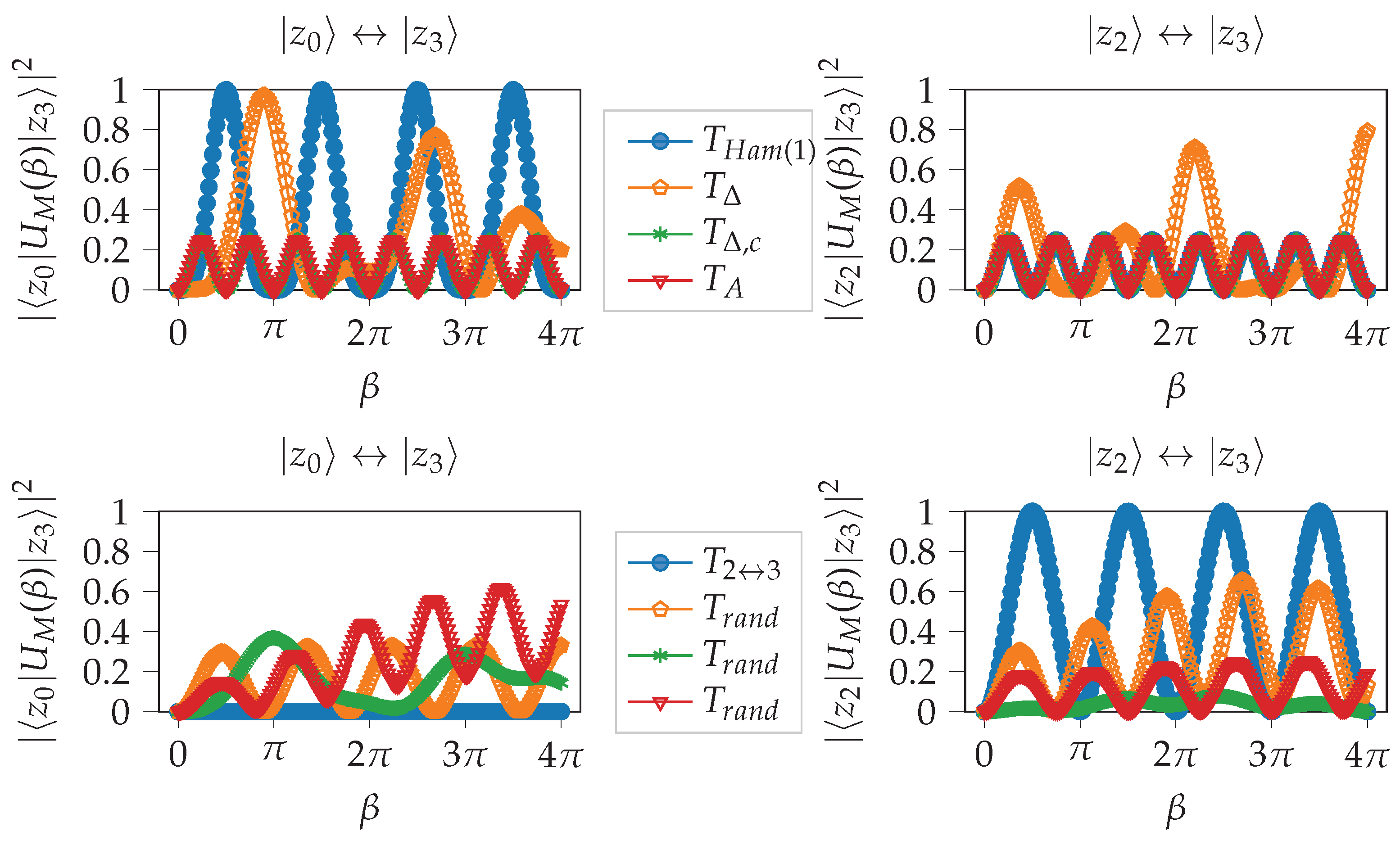
is independent of the elements in B. This allows us to describe and analyze valid transition matrices by only knowing the number of feasible states, i.e., . What these specific states are is irrelevant, unless one wants to look at what an optimal mixer is, which we will come back to in Section 3.4. Figure 3 provides a comparison of some mixers described in the following with respect to the overlap between different states.
In the following, we denote the matrix for pairs of indices whose binary representation have a Hamming distance equal to d as
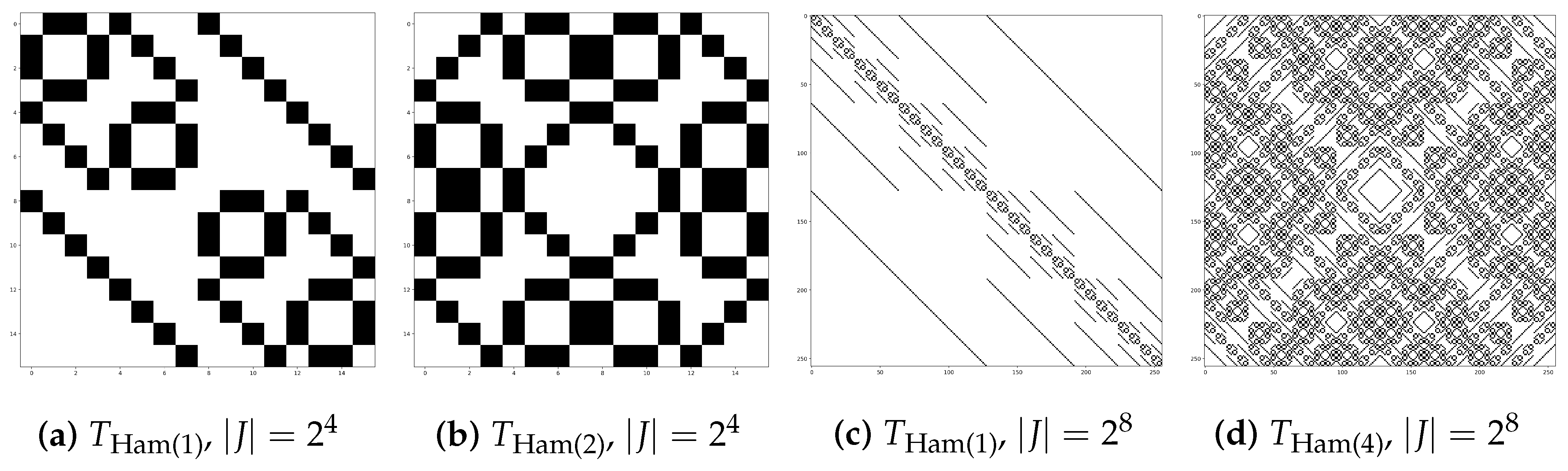
Examples of the structure of can be found in Figure 4.
Furthermore, it will be useful to denote the matrix which has two nonzero entries at and as
Before we start, we point out that the diagonal entries of T can be chosen to be zero, because for all . Although trivial, we will repeatedly use that is an eigenvector of a matrix if the sum of all rows are a multiple of v.
3.2.1. Hamming Distance One Mixer
The matrix fulfills Theorem 1 when . The symmetry of is due to the fact that the Hamming distance is a symmetric function. Using the identity
it can be shown that
where are real coefficients. Therefore, it is clear that reaches all states with Hamming distance K. Furthermore, is a unit eigenvector of since the sum of each row is n. This is because there are exactly n other states with a Hamming distance of one for each bitstring.
3.2.2. All-to-All Mixer
We denote the matrix with all but the diagonal entries equal to one as
Trivially, fulfilles Theorem 1 and is a unit eigenvector of since the sum of each row is .
3.2.3. (Cyclic) Nearest Integer Mixer /
Inspired by the stencil of finite-difference methods, we introduce , as matrices with off-diagonal entries equal to one
Both matrices fulfill Theorem 1. Symmetry holds by definition, and it is easy to see that the k-th off-diagonal of and is nonzero for .
For the nearest integer mixer , it is known that
are eigenvectors for . For the cyclic nearest integer mixer, we have that the sum of each row/column of is equal to two (except for when it is one). Therefore, is a unit eigenvector.
3.2.4. Products of Mixers and
In some cases, it will be necessary to use Theorem 2 to implement mixer unitaries. When splitting transitions matrices into odd and even entries, the following definition is useful. Denote the matrix with entries in the d-th off-diagonal for even rows equal to one
and accordingly for odd rows. In addition, we will use to be the cyclic version in the same way as in Equation (28). As an example, this allows one to decompose with and .
3.2.5. Random Mixer
Finally, the upper triangular entries of the mixer are drawn from a continuous uniform distribution on the interval , and the lower triangular entries are chosen such that T becomes symmetric. Since the probability of getting a zero entry is zero, such a random mixer fulfills Theorem 1 with probability 1.
3.3. Decomposition of (Constraint) Mixers into Basis Gates
Given a set of feasible (computational basis) states , we can use Theorem 1 to define a suitable mixer Hamiltonian. The next question is how to (efficiently) decompose the resulting mixer into basis gates. In order to do so, we first decompose the Hamiltonian into a weighted sum of Pauli-strings. A Pauli-string P is a Hermitian operator of the form where . Pauli-strings form a basis of the real vector space of all n-qubit Hermitian operators. Therefore, we can write
with real coefficients , where . After using a standard Trotterization scheme [4,5] (which is exact for commuting Pauli-strings),
it is well-established how to implement each of the terms of the product using basis gates; see Equation (33). We will discuss the effects of Trotterization in more detail in Section 3.5, as there are several important aspects to consider for a valid mixer.
![Algorithms 15 00202 i004]()

Here, S is the S or Phase gate and H is the Hadamard gate. The standard way to compute the coefficients is given in Algorithm 1.
| Algorithm 1: Decompose given by Equation (10) into Pauli-strings via trace |
 |
For n qubits, this requires to compute coefficients, as well as the multiplication of matrices. However, most of these terms are expected to vanish. We therefore describe an alternative way to produce this decomposition, using the language of quantum mechanics [24]. In the following, we use the ladder operators used in the creation and annihilation operators from the second quantization formulation in quantum chemistry defined by
Since , where 0 is the zero vector, we have that . Since , we have that , and finally means that and . Note that
As an example, consider the matrix , which can be expressed with ladder operators as . Another example is given by . This approach clearly extends to the general case and leads to Algorithm 2.
| Algorithm 2: Decompose given by Equation (10) into Pauli-strings directly |
 |
A comparison of the complexity of the two algorithms is given in Table 1. The naive algorithm needs to perform a matrix–matrix multiplication with matrices of size for each of the coefficients. This quickly becomes prohibitive for larger n. The algorithm based on ladder operators requires resources that scale with the number of nonzero entries of the transition matrix T, which is much more favorable. In the end, a symbolic mathematics library is used to simplify the expressions in order to create the list of nonzero Pauli-strings.
3.4. Optimality of Mixers
On current NISQ devices, the noise level of two-qubit gate (CX) times and error rates are one order of magnitude higher than for single qubit gates (). In addition, most devices lack all-to-all connectivity. The CX gates between these require SWAP operations, which consist of additional CX gates. An optimal mixer will therefore contain as few CX gates as possible. Since Pauli-strings are implemented according to Equation (33), we define the cost to implement as
where is the length of a Pauli-string P defined as the number of literals that are not the identity. For instance, has . The specifies the number of CX gates that are required to implement the mixer. A lower cost means fewer and/or shorter Pauli-strings. There are four interconnected factors that influence the cost to implement the mixer for a given B.
3.4.1. Transition Matrix T
The larger , the more freedom we have in choosing the transition matrix T that fulfills Theorem 1. The combination of T and the specific states of B define the cost of the Hamiltonian. Unless one can find a way to utilize the structure of the states of B to efficiently compute an optimal T, we expect this problem to be NP-hard. In practice, a careful analysis of the specific states of B is required to determine T such that the cost becomes low. We will revisit optimality for both unrestricted and restricted mixers in Section 4 and Section 5.
3.4.2. Adding Mixers
Corollary 2 allows one to add mixers with a kernel that contains . In general, also, this is a combinatorial optimization problem which we do not expect to solve exactly with an efficient algorithm. However, we will provide a heuristic that can be used to reduce the cost of mixers in certain cases. We will provide more details in Section 5 where we discuss constrained mixers on some examples in detail.
3.4.3. Non-Commuting Pauli-Strings
Depending on the mixer—which depends on the transition matrix and addition of mixers outside the feasible subspace—one can influence the commutativity pattern of the resulting Pauli-strings. This is an intricate topic, which we discuss next.
3.5. Trotterizations
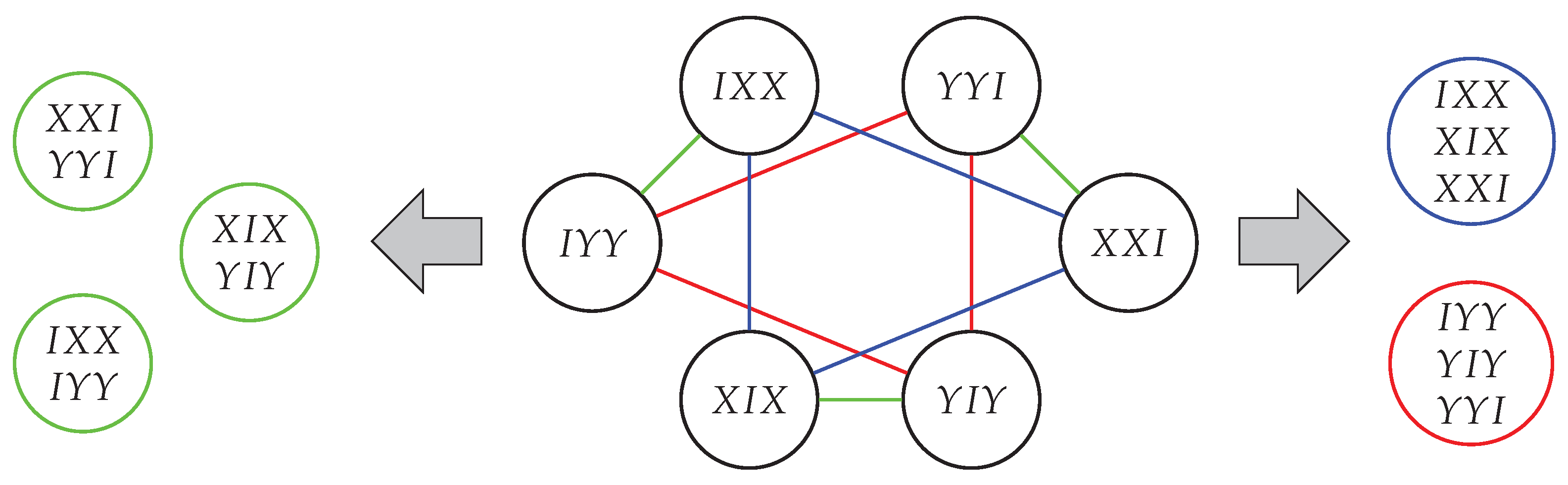
Algorithms 1 and 2 produce a weighted sum of Pauli-strings equal to the mixer Hamiltonian defined in Theorem 1. A further complication arises when the non-vanishing Pauli-strings of the mixer Hamiltonian do not all commute. In that case, one can not realize exactly but has to find a suitable approximation/Trotterization; see Equation (32). Two Pauli-strings commute, i.e., if, and only if, they fail to commute on an even number of indices [25]. An example is given in Figure 5.
This problem is similar to a problem for observables: how does one divide the Pauli-strings into groups of commuting families [25,26] to maximize efficiency and increase accuracy? In order to minimize the number of measurements required to estimate a given observable, one wants to find a “min-commuting-partition”; given a set of Pauli-strings from a Hamiltonian, one seeks to partition the strings into commuting families such that the total number of partitions is minimized. This problem is NP-hard in general [25]. However, based on Theorem 3, we expect our problem to be much more tractable.
For our case, it turns out that not all Trotterizations are suitable as mixing operators; they can either fail to preserve the feasible subspace, i.e., Equation (5), or fail to provide transitions between all pairs of feasible states, i.e., Equation (6). An example is given by with the mixer associated with ; see Section 5.1. Looking at Figure 5, these terms can be grouped into commuting families in two ways, which represent two (of many) different ways to realize the mixer unitary with basis gates.
- The first possible Trotterization is given by and . However, it turns out that such that for all . This means that this Trotterization does not preserve the feasible subspace and does not represent a valid mixer Hamiltonian. The underlying reason for this is that the terms and are generated from the entry , but are split in this Trotterization. The same holds true for and , which are generated via .
- The second possible Trotterization is given by and , which splits terms with respect to and In this case, we have that , so it does not provide an overlap between all feasible computational basis states. This can be understood via Theorem 2. We have that for all , so one can not “reach” |100⟩ from |001⟩. The opposite is not true; we have that , so such that .
We have just learned that it is a bad idea to Trotterize terms that belong to a nonzero entry of T, i.e., to . Therefore, we need to show that all non-vanishing Pauli-strings of commute; otherwise, there might exist subspaces for which we can not realize the mixer constructed in Theorem 1. Luckily, the following theorem shows that it is always possible to realize a mixer by Trotterizing according to nonzero entries of .
Theorem 3
(Pauli-strings for commute). Let be two computational basis states in . Then, all non-vanishing Pauli-strings of the decomposition
commute.
Proof.
We will prove the following more general assertion by induction. Let be two non-vanishing Pauli-strings of the decomposition of , and be two non-vanishing Pauli-strings of the decomposition of . Then, , and . We will use that two Pauli-strings commute if, and only if, they fail to commute on an even number of indices [25].
For , we have the following cases.
It is trivially true that and , since the maximum number of Pauli-strings is two, and in that case, one of the Pauli-strings is the identity. Moreover, is nonzero only when . In that case, .
. We assume the assumptions hold for two computational basis states . Then, there are the following four cases
where .
Case . According to our assumptions that all non-vanishing Pauli-strings for commute, the same holds for . Since , the rest of the assertions are trivially true, as there are no non-vanishing Pauli-strings.
Case . Our assumptions mean that non-vanishing Pauli-strings of fail to commute on an odd number of indices with non-vanishing Pauli-strings of . Therefore, non-vanishing Pauli-strings of fail to commute on an even number of indices, and, hence, commute. The same argument holds for . Finally, we prove that non-vanishing Pauli-strings of and do not commute. Either Pauli strings and stem from and , respectively, or they stem from and , respectively. In both cases, the number of commuting terms does not change, so non-vanishing Pauli-strings of and do not commute. □
The proof in Theorem 3 inspires the following algorithm to decompose into Pauli-strings. For each item in the list S that the algorithm produces, all Pauli-strings commute.
We can illustrate the difference between Algorithms 2 and 3 for and . With Algorithm 2, we have and , which can be simplified to . With Algorithm 3, we have and without the need to simplify the expression.
| Algorithm 3: Decompose given by Equation (10) into Pauli-strings directly |
 |
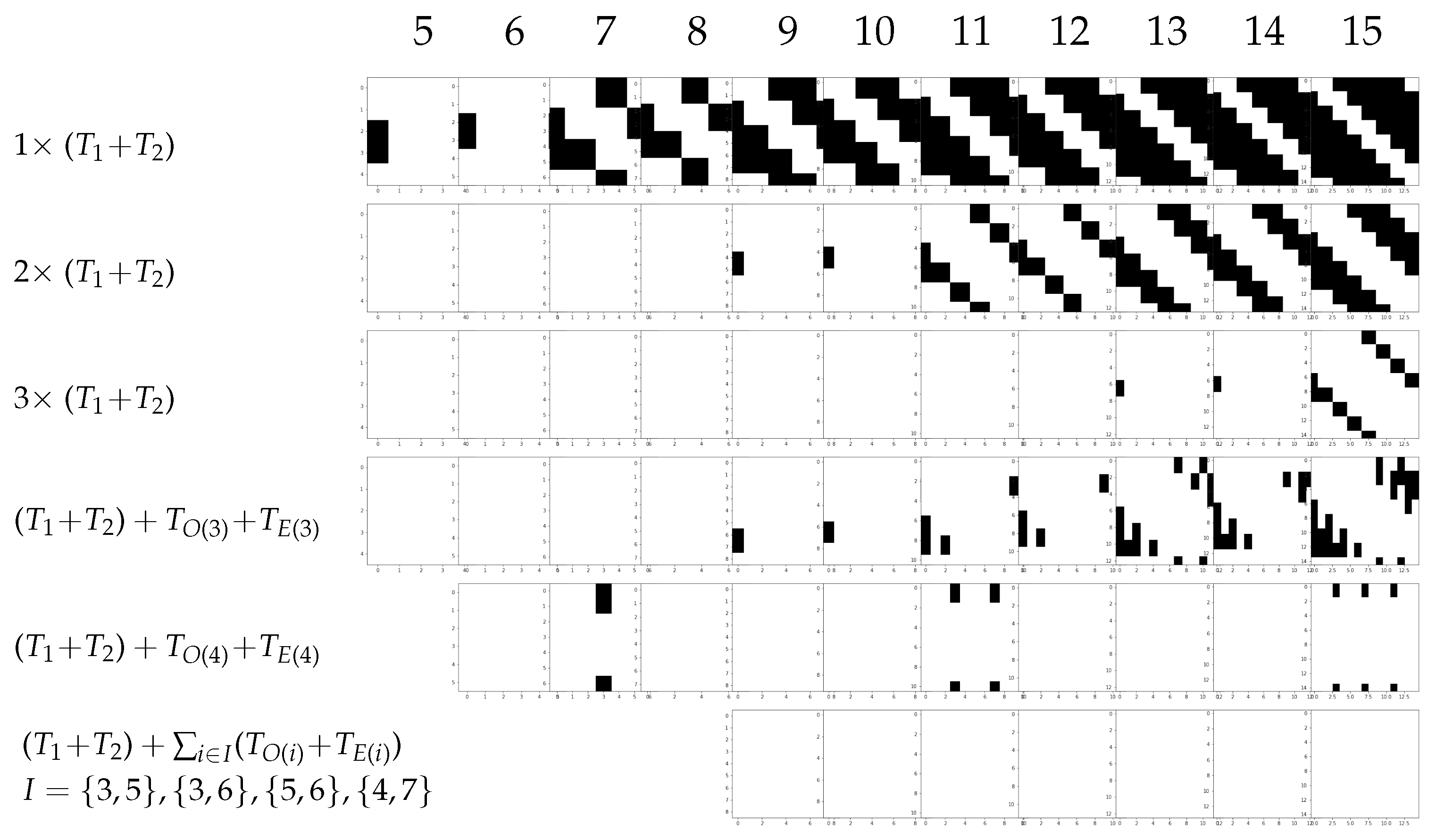
As shown above, Trotterizations can also lead to missing transitions. It is suggested in [2] that it is useful to repeat mixers within one mixing step, which corresponds to in Equation (6). However, as we see in Figure 6, there can be more efficient ways to obtain mixers that provide transitions between all pairs of feasible states. One way to do so is to construct an exact Trotterization (restricted to the feasible subspace) as described in [19]. However, the ultimate goal is not to avoid Trotterization errors, but rather to provide transitions between all pairs of feasible states. We will revisit the topic of Trotterizations in Section 5 in more detail for each case and show that there are more efficient ways to do so.
4. Full/Unrestricted Mixer
We start by applying the proposed algorithm to the case without constraints, i.e., for the case in Equation (1), in order to check for consistency and new insight. We will see that the presented approach is able to reproduce the “standard” X mixer as one possibility, but it provides a more general framework. For this case, , , which means that . Furthermore, using Equation (14), we have that , since E is the identity.
4.1. aka “Standard” Full Mixer
The Hamiltonian of the standard full mixer for n qubits can be written as
The last identity in Equation (40) shows that is created by the transition matrix given by . This assumes that the feasible states in B are ordered from the smallest to the largest integer representation.
4.2. All-to-All Full Mixer
For , the full mixer can be written as . For the case , the resulting Hamiltonian does not provide transitions between all pairs of feasible states, but we observe that , i.e., consists of all possible pairs of Pauli-strings, which contain exactly two Xs. For , this can be further generalized to
which consists of all possible pairs of Pauli-strings with exactly m Xs. The resulting mixer Hamiltonian is therefore given by
This means that the mixer consists of the standard mixer plus applications of Pauli X-k strings for k from 2 to n, which is a large overhead compared to the standard X-mixer.
4.3. (Cyclic) Nearest Integer Full Mixer
The resulting mixer for / involves exponentially many Pauli-strings with increasing n. The following shows for .
4.4. Comparison and Optimality of Full Mixers
It would be convenient to have a condition on the transition matrix for the optimality of the resulting mixer. We define the total Hamming distance of T to be
where is the binary representation of an integer i. As a first instinct, one might suspect that the mixer with minimal Hamming distance also minimizes the cost. However, this turns out to be false because of cancellations when more terms in T are nonzero. Table 2 gives a comparison of the total Hamming distance and cost for different full mixers. The standard full mixer has a total Hamming distance , as there are states each with states that have a Hamming distance of 1. The all-to-all full mixer has . For the rest of the transition matrices, it is not that straightforward to derive a general formula for , but the table gives an impression. Table 2 shows a dramatic difference between the different mixers with regard to resource requirements. The standard mixer is the only one that does not require CX gates and is the most efficient to implement. Furthermore, as the resulting Pauli terms for the full mixers given by and consist only of I and X and therefore commute, they can be implemented without Trotterization. For the mixers given by , and , on the other hand, not all Pauli-strings commute, which results in the need for Trotterization. We continue with the case of constrained mixers.
5. Constrained Mixers
We start by describing what is known as the “XY”-mixer [2,17,19] before we explore more general cases. Our framework provides additional insights into this case and inspires further improvement of the algorithms above with respect to the optimality of the mixers, described in Section 3.4, by (possibly) reducing the length of Pauli-strings. For this case, we will analyze , and only. only makes sense when n is a power of two, and has in general high cost; see Table 2.
5.1. “One-Hot” Aka “XY”-Mixer
We are concerned with the case given by all computational basis states with exactly one “1”, i.e., . These states are sometimes referred to as “one-hot”. We have that is the number of qubits. After some motivating examples, we present the general case for constructing mixers for any .
5.1.1. Case
The smallest, non-trivial case is given by . For any , the transition matrix fulfills Theorem 1 and leads to the mixer . Since we want to minimize given in Equation (36), we set , which results in the . However, by using Corollary 2, there is room for further reducing the cost. We can add the mixer for , since . Using the same T (setting ) gives
which has . No Trotterization is needed in this case.
5.1.2. Case
We continue with . For the transition matrix , this results in the mixer
with associated cost for . In this case, Corollary 2 allows us to add the mixer for since . The mixer
has cost for . However, this mixer can not be realized, since not all terms of commute. Figure 5 shows two ways to put the graph into commuting Pauli-terms with only one way to preserve the feasible subspace, as discussed in Section 3.5. For the Trotterization according to , we have that . To fulfill Theorem 2, we need to include the term as well. The Trotterized mixer with minimal cost is therefore given by .
5.1.3. The General Case
We start with the observation that for any symmetric with zero diagonal, we have
The cost for implementing one of the entries, i.e., is given by the recursive formula
where is Pascal’s triangle starting with 2 instead of 1. Examples of the resulting costs for different transition matrices can be seen in Table 3.
The cost of the mixers can be considerably reduced by adding mixers generalized from case . If the entries of T are nonzero, we can add mixers for each of the pairs of states that fulfill that . We can enumerate them with by , where removes the indices i and j of x. We have that . We observe that for , let with , i.e., the strings differ at exactly two positions we have that
Adding these mixers for each nonzero entry of T has the effect of summing over all possible combinations of , which is equal to the identity. Therefore, we obtain the mixer
which reduces the cost of one term to .
5.1.4. Trotterizations
Not all Pauli-strings of the mixer in Equation (51) commute. This necessitates a suitable and efficient Trotterization. We will use Theorems 2 and 3 to identify valid Trotterized mixers. As pointed out in [19], when n is a power of two, one can realize a Trotterization, which is exact in the feasible subspace B. Termed simultaneous complete-graph mixer, this involves all possible pairs corresponding to a certain Trotterization of mixer for . We will see that there are more efficient mixers that provide transitions between all pairs of feasible states.
Another possibility is to Trotterize or according to odd and even entries as described in Section 3.2.4. This is what is termed a parity-partitioned mixer in [19]. However, fewer and fewer feasible states can be reached as n increases, as we have seen in Figure 6. Repeated applications ( in Equation (6)) are necessary, and r increases with increasing n. Figure 7 shows a comparison of different Trotterizations. As the cost of the mixer is dictated by the number of nonzero entries of the transition matrix, it is more efficient to add mixers for off-diagonals according to for some suitable index set I.
5.2. General Cases
In this section, we analyze some specific cases that go beyond unrestricted mixers and mixers restricted to one-hot states.
5.2.1. Example 1
We start by looking at the case . Using and , this results in the mixer
with . Here, corresponds to and to . There is a lot of freedom adding mixers, which is summarized in Table 4. Adding more terms only increases the cost for this case. Overall, the most efficient mixers for B are given by
with associated cost . A valid Trotterization is given through splitting according to .
5.2.2. Example 2
Finally, we investigate the case , which restricts to six of the total computational basis states for 5 qubits. It is not clear a priori if for any (distinct) pair and , all pairs of non-vanishing Pauli strings commute. In order to fulfill Equation (6) for , this means that one needs to Trotterize according to all pairs of , as shown in Table 5. The resulting cost for this Trotterized mixer is . Since is spanned by computational basis states, there are different pairs to add to each . As Table 5 shows, this can reduce the cost of the resulting mixer to . Of course, there is the possibility to reduce the cost even further by adding more mixers for states in the kernel of . However, this quickly becomes computationally very demanding, when all possibilities are considered in a brute-force fashion.
6. Conclusions and Outlook
While designing mixers with the presented framework is more or less straightforward, designing efficient mixers turns out to be a difficult task. An additional difficulty arises due to the need for Trotterization. Somewhat counter-intuitively, the more restricted the mixer, i.e., the smaller the subspace, the more design freedom one has to increase efficiency. More structure/symmetry of the restricted subspace seems to allow for a lower cost of the resulting mixer. For the case of “one-hot” states, we provide a deeper understanding of the requirements for Trotterizations. Compared to the state of the art in the literature, this leads to a considerable reduction of the cost of the mixer, as defined in Equation (36). The introduced framework reveals a rigorous mathematical analysis of the underlying structure of mixer Hamiltonians and deepens the understanding of those. We believe the framework can serve as the backbone for the further development of efficient mixers.
When adding mixers, in general, the kernel of is spanned by computational basis states. Therefore, one can add
different mixers for each nonzero entry of T. Out of all these, one wants to find the combination leading to the lowest overall cost. Clearly, brute-force optimization is computationally not tractable, even for a moderate number of qubits n when . Further research should aim to carefully analyze the structure of the basis states in B in order to develop efficient (heuristic) algorithms to find low-cost mixers through adding mixers in the kernel of .
Author Contributions
Conceptualization, F.G.F., K.O.L., H.M.N., A.J.S. and G.S.; software, F.G.F.; formal analysis, F.G.F.; data curation, F.G.F.; writing—original draft preparation, F.G.F.; writing—review and editing, F.G.F., K.O.L., H.M.N., A.J.S. and G.S.; visualization, F.G.F. All authors have read and agreed to the published version of the manuscript.
Funding
This research received no external funding.
Institutional Review Board Statement
Not applicable.
Informed Consent Statement
Not applicable.
Data Availability Statement
All data and the python/jupyter notebook source code for reproducing the results obtained in this article are available at https://github.com/OpenQuantumComputing as of 1 June 2022.
Conflicts of Interest
The authors declare no conflict of interest.
References
- Farhi, E.; Goldstone, J.; Gutmann, S. A quantum approximate optimization algorithm. arXiv 2014, arXiv:1411.4028. [Google Scholar]
- Hadfield, S.; Wang, Z.; O’Gorman, B.; Rieffel, E.G.; Venturelli, D.; Biswas, R. From the quantum approximate optimization algorithm to a quantum alternating operator ansatz. Algorithms 2019, 12, 34. [Google Scholar] [CrossRef]
- Lucas, A. Ising formulations of many NP problems. Front. Phys. 2014, 2, 5. [Google Scholar] [CrossRef]
- Hatano, N.; Suzuki, M. Finding exponential product formulas of higher orders. In Quantum Annealing and Other Optimization Methods; Springer: Berlin/Heidelberg, Germany, 2005; pp. 37–68. [Google Scholar]
- Trotter, H.F. On the product of semi-groups of operators. Proc. Am. Math. Soc. 1959, 10, 545–551. [Google Scholar] [CrossRef]
- Kronsjö, L. Algorithms: Their Complexity and Efficiency; John Wiley & Sons, Inc.: Hoboken, NJ, USA, 1987. [Google Scholar]
- Guerreschi, G.G.; Matsuura, A. QAOA for Max-Cut requires hundreds of qubits for quantum speed-up. Sci. Rep. 2019, 9, 6903. [Google Scholar] [CrossRef]
- Cerezo, M.; Arrasmith, A.; Babbush, R.; Benjamin, S.C.; Endo, S.; Fujii, K.; McClean, J.R.; Mitarai, K.; Yuan, X.; Cincio, L.; et al. Variational quantum algorithms. Nat. Rev. Phys. 2021, 3, 625–644. [Google Scholar] [CrossRef]
- Moll, N.; Barkoutsos, P.; Bishop, L.S.; Chow, J.M.; Cross, A.; Egger, D.J.; Filipp, S.; Fuhrer, A.; Gambetta, J.M.; Ganzhorn, M.; et al. Quantum optimization using variational algorithms on near-term quantum devices. Quantum Sci. Technol. 2018, 3, 030503. [Google Scholar] [CrossRef]
- Bittel, L.; Kliesch, M. Training variational quantum algorithms is NP-hard—Even for logarithmically many qubits and free fermionic systems. Phys. Rev. Lett. 2021, 127, 120502. [Google Scholar] [CrossRef]
- Wang, S.; Fontana, E.; Cerezo, M.; Sharma, K.; Sone, A.; Cincio, L.; Coles, P.J. Noise-induced barren plateaus in variational quantum algorithms. Nat. Commun. 2021, 12, 1–11. [Google Scholar] [CrossRef]
- Zhang, H.K.; Zhu, C.; Liu, G.; Wang, X. Fundamental limitations on optimization in variational quantum algorithms. arXiv 2022, arXiv:2205.05056. [Google Scholar]
- Zhu, L.; Tang, H.L.; Barron, G.S.; Mayhall, N.J.; Barnes, E.; Economou, S.E. An adaptive quantum approximate optimization algorithm for solving combinatorial problems on a quantum computer. arXiv 2020, arXiv:2005.10258. [Google Scholar]
- Bravyi, S.; Kliesch, A.; Koenig, R.; Tang, E. Obstacles to state preparation and variational optimization from symmetry protection. arXiv 2019, arXiv:1910.08980. [Google Scholar]
- Egger, D.J.; Marecek, J.; Woerner, S. Warm-starting quantum optimization. arXiv 2020, arXiv:2009.10095. [Google Scholar] [CrossRef]
- Vikstål, P.; Grönkvist, M.; Svensson, M.; Andersson, M.; Johansson, G.; Ferrini, G. Applying the Quantum Approximate Optimization Algorithm to the Tail-Assignment Problem. Phys. Rev. Appl. 2020, 14, 034009. [Google Scholar] [CrossRef]
- Fuchs, F.G.; Kolden, H.; Aase, N.H.; Sartor, G. Efficient Encoding of the Weighted MAX k-CUT on a Quantum Computer Using QAOA. SN Comput. Sci. 2021, 2, 1–14. [Google Scholar] [CrossRef]
- Hadfield, S.; Wang, Z.; Rieffel, E.G.; O’Gorman, B.; Venturelli, D.; Biswas, R. Quantum approximate optimization with hard and soft constraints. In Proceedings of the Second International Workshop on Post Moores Era Supercomputing, Denver, CO, USA, 12–17 November 2017; pp. 15–21. [Google Scholar]
- Wang, Z.; Rubin, N.C.; Dominy, J.M.; Rieffel, E.G. XY mixers: Analytical and numerical results for the quantum alternating operator ansatz. Phys. Rev. A 2020, 101, 012320. [Google Scholar] [CrossRef]
- Lieb, E.; Schultz, T.; Mattis, D. Two soluble models of an antiferromagnetic chain. Ann. Phys. 1961, 16, 407–466. [Google Scholar] [CrossRef]
- Cook, J.; Eidenbenz, S.; Bärtschi, A. The quantum alternating operator ansatz on maximum k-vertex cover. In Proceedings of the 2020 IEEE International Conference on Quantum Computing and Engineering (QCE), Broomfield, CO, USA, 12–16 October 2020; IEEE: Piscataway, NJ, USA, 2020; pp. 83–92. [Google Scholar]
- Hen, I.; Sarandy, M.S. Driver Hamiltonians for constrained optimization in quantum annealing. Phys. Rev. A 2016, 93, 062312. [Google Scholar] [CrossRef]
- Hen, I.; Spedalieri, F.M. Quantum annealing for constrained optimization. Phys. Rev. Appl. 2016, 5, 034007. [Google Scholar] [CrossRef]
- Sakurai, J.J. Advanced Quantum Mechanics; Pearson: Upper Saddle River, NJ, USA, January 1967. [Google Scholar]
- Gokhale, P.; Angiuli, O.; Ding, Y.; Gui, K.; Tomesh, T.; Suchara, M.; Martonosi, M.; Chong, F.T. Minimizing state preparations in variational quantum eigensolver by partitioning into commuting families. arXiv 2019, arXiv:1907.13623. [Google Scholar]
- Gui, K.; Tomesh, T.; Gokhale, P.; Shi, Y.; Chong, F.T.; Martonosi, M.; Suchara, M. Term grouping and travelling salesperson for digital quantum simulation. arXiv 2020, arXiv:2001.05983. [Google Scholar]
Figure 1.
Illustration of properties of Hamiltonians constructed with Theorem 1.

Figure 2.
Corollary 2 shows that adding a mixer with support outside is also a valid mixer for B.

Figure 3.
Examples of the squared overlap between two states for the case . The squared overlap is independent of what the states in are. The comparison for different T shows that there exists a such that the overlap is nonzero, except for which, as expected, does not provide transitions between and .

Figure 4.
Examples of the structure of . The black color represents non-vanishing entries equal to one, representing pairs with the specified Hamming distance.
Figure 4.
Examples of the structure of . The black color represents non-vanishing entries equal to one, representing pairs with the specified Hamming distance.

Figure 5.
In the commutation graph (middle) of the terms of the mixer given in Equation (47), an edge occurs if the terms commute. From this, we can group terms into three (nodes connected by green edge) or two (nodes connected by red/blue edges) sets. Only the left/green grouping preserves the feasible subspace, the right one does not.

Figure 6.
Valid (white) and invalid (black) transitions between pairs of states, as defined in Theorem 2 for Trotterized mixer Hamiltonians. The first row shows that for and , the mixer does not provide transitions between all pairs of feasible states, although does.
Figure 6.
Valid (white) and invalid (black) transitions between pairs of states, as defined in Theorem 2 for Trotterized mixer Hamiltonians. The first row shows that for and , the mixer does not provide transitions between all pairs of feasible states, although does.

Figure 7.
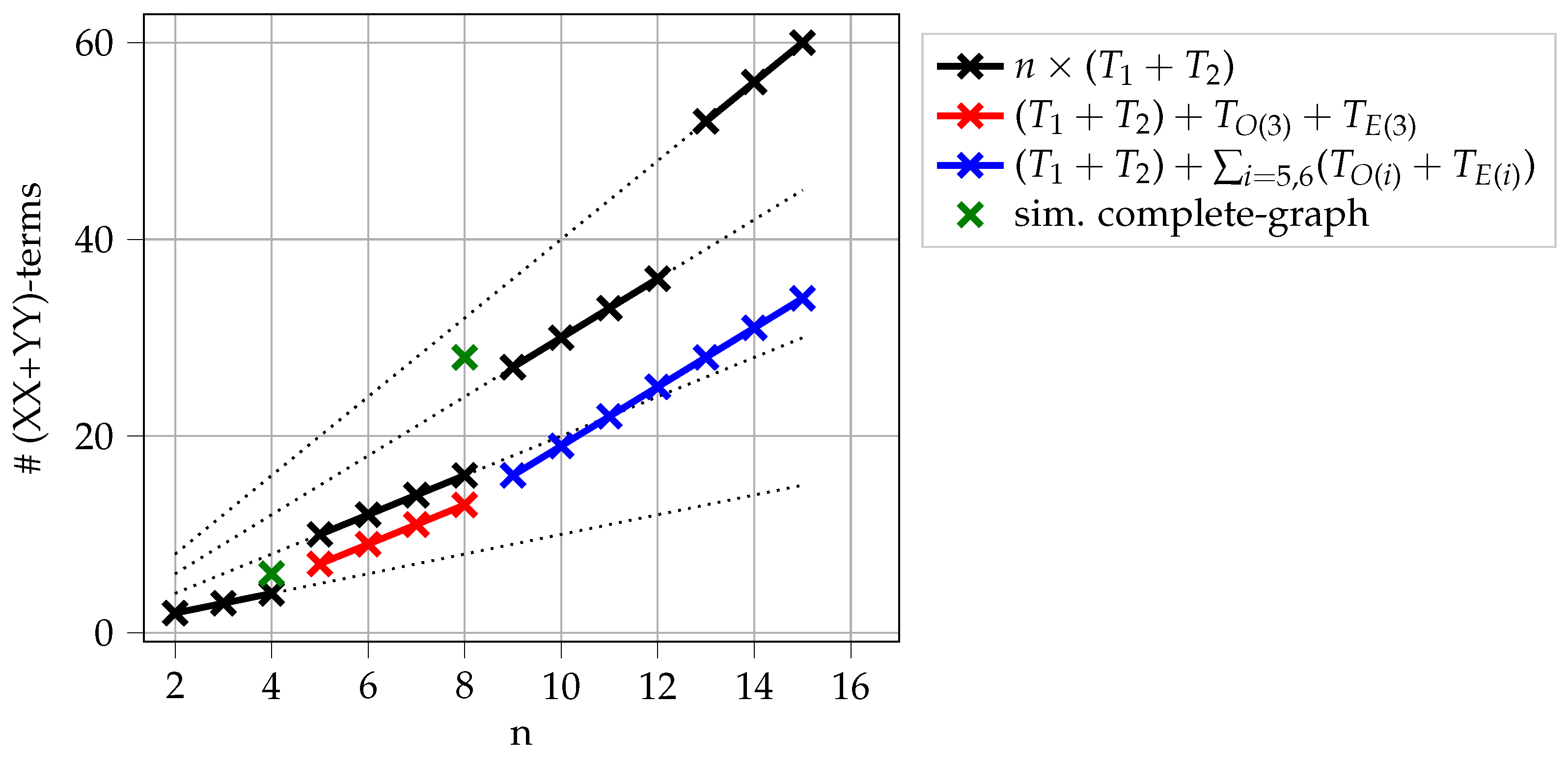
Comparison of different Trotterization mixers restricted to “one-hot” states. All markers represent cases when the resulting mixer provides transitions for all pairs of feasible states; see also Figure 6. All versions can be implemented in linear depth. The most efficient Trotterizations are achieved by using sub-diagonal entries. The cost equals 4 times # (XX + YY)-terms.
Figure 7.
Comparison of different Trotterization mixers restricted to “one-hot” states. All markers represent cases when the resulting mixer provides transitions for all pairs of feasible states; see also Figure 6. All versions can be implemented in linear depth. The most efficient Trotterizations are achieved by using sub-diagonal entries. The cost equals 4 times # (XX + YY)-terms.


Table 1.
Comparison of the complexity of the two algorithms for n qubits. Here, is the number of nonzero entries of T.
Table 1.
Comparison of the complexity of the two algorithms for n qubits. Here, is the number of nonzero entries of T.
| Algorithm 1 | Algorithm 2 | Algorithm 3 | |
|---|---|---|---|
| runtime | |||
| memory |
Table 2.
Full/unrestricted mixer case for n qubits, i.e., . Comparison of the total Hamming distance of the transition matrix T as well as resulting requirements for implementations in terms of single- and two-qubit gates for different T.
Table 2.
Full/unrestricted mixer case for n qubits, i.e., . Comparison of the total Hamming distance of the transition matrix T as well as resulting requirements for implementations in terms of single- and two-qubit gates for different T.
| n | 1 | 2 | 3 | 4 | 5 | 6 | 1 | 2 | 3 | 4 | 5 | 6 | 1 | 2 | 3 | 4 | 5 | 6 |
|---|---|---|---|---|---|---|---|---|---|---|---|---|---|---|---|---|---|---|
| Ham | # | #CX | ||||||||||||||||
| 2 | 8 | 24 | 64 | 160 | 384 | 1 | 2 | 3 | 4 | 5 | 6 | 0 | 0 | 0 | 0 | 0 | 0 | |
| 2 | 16 | 96 | 512 | 2560 | 12,288 | 1 | 2 | 3 | 4 | 5 | 6 | 0 | 2 | 10 | 34 | 98 | 258 | |
| 2 | 12 | 28 | 60 | 124 | 252 | 1 | 1 | 1 | 1 | 1 | 1 | 0 | 2 | 12 | 44 | 132 | 356 | |
| 2 | 8 | 22 | 52 | 114 | 240 | 1 | 1 | 1 | 1 | 1 | 1 | 0 | 4 | 20 | 68 | 196 | 516 | |
| 2 | 16 | 96 | 512 | 2560 | 12,288 | 2 | 4 | 6 | 8 | 10 | 12 | 0 | 10 | 86 | 552 | 3260 | 17,650 | |
Table 3.
Comparison of the cost #CX of mixers constrained to “one-hot” states. The Trotterized versions we define and . All Hamiltonians need to be Trotterized.
Table 3.
Comparison of the cost #CX of mixers constrained to “one-hot” states. The Trotterized versions we define and . All Hamiltonians need to be Trotterized.
| n | 3 | 4 | 5 | 6 | 7 | 8 | 9 | 10 | 15 |
|---|---|---|---|---|---|---|---|---|---|
| 12 · 2 | 32 · 3 | 80 · 44 | 192 · 54 | 448 · 64 | 1024 · 74 | 2304 · 84 | 5120 · 94 | 245,760 · 144 | |
| 12 · 3 | 32 · 4 | 80 · 54 | 192 · 64 | 448 · 74 | 1024 · 84 | 2304 · 94 | 5120 · 10 | 245,760 · 154 | |
| 12 · 3 | 32 · 6 | 80 · 10 | 192 · 15 | 448 · 21 | 1024 · 28 | 2304 · 36 | 5120 · 45 | 245,760 · 105 | |
| 4 · 2 | 4 · 3 | 4 · 44 | 4 · 54 | 4 · 64 | 4 · 74 | 4 · 84 | 4 · 94 | 4 · 144 | |
| 4 · 3 | 4 · 4 | 4 · 54 | 4 · 64 | 4 · 74 | 4 · 84 | 4 · 94 | 4 · 10 | 4 · 154 | |
| 4 · 3 | 4 · 6 | 4 · 10 | 4 · 15 | 4 · 21 | 4 · 28 | 4 · 36 | 4 · 45 | 4 · 105 | |
Table 4.
Comparison of the for different added mixers C for the case . All 10 possible pairs are shown. We see that the cost can be both reduced and increased.
Table 4.
Comparison of the for different added mixers C for the case . All 10 possible pairs are shown. We see that the cost can be both reduced and increased.
| 12 | 8 | 16 | |
| 20 | 2 | 24 | |
| 24 | 20 | 28 | |
| 6 | 20 | 28 | |
| 28 | 24 | 8 | |
| 20 | 16 | 24 | |
| 28 | 24 | 8 | |
| 6 | 20 | 28 | |
| 24 | 20 | 28 | |
| 20 | 16 | 24 | |
| 20 | 2 | 24 |
Table 5.
Comparison of the for different added mixers C for the case . There are 325 possible pairs in total. We see that the cost can be both reduced and increased.
Table 5.
Comparison of the for different added mixers C for the case . There are 325 possible pairs in total. We see that the cost can be both reduced and increased.
| 96 | 64 | 112 | 80 | 80 | 112 | 96 | 64 | 64 | 96 | 96 | 96 | 112 | 112 | 80 | |
| 160 | 24 | 176 | 144 | 144 | 176 | 160 | 128 | 128 | 160 | 160 | 160 | 176 | 176 | 144 | |
| 208 | 176 | 48 | 192 | 192 | 224 | 208 | 176 | 176 | 208 | 208 | 208 | 224 | 224 | 192 | |
| 192 | 160 | 208 | 176 | 176 | 208 | 48 | 160 | 160 | 192 | 192 | 192 | 208 | 208 | 176 | |
| 208 | 176 | 224 | 192 | 192 | 224 | 208 | 176 | 176 | 208 | 208 | 208 | 224 | 48 | 192 | |
| 208 | 176 | 224 | 192 | 192 | 224 | 208 | 176 | 176 | 208 | 208 | 208 | 48 | 224 | 192 | |
| 192 | 160 | 208 | 176 | 176 | 208 | 192 | 160 | 160 | 40 | 192 | 192 | 208 | 208 | 176 | |
| 192 | 160 | 208 | 176 | 176 | 208 | 48 | 160 | 160 | 192 | 192 | 192 | 208 | 208 | 176 | |
| 176 | 144 | 192 | 160 | 160 | 192 | 176 | 144 | 144 | 176 | 176 | 176 | 192 | 192 | 32 | |
| 160 | 128 | 176 | 144 | 144 | 176 | 160 | 24 | 128 | 160 | 160 | 160 | 176 | 176 | 144 | |
| 176 | 144 | 192 | 32 | 160 | 192 | 176 | 144 | 144 | 176 | 176 | 176 | 192 | 192 | 160 | |
| 192 | 160 | 208 | 176 | 176 | 208 | 192 | 160 | 160 | 192 | 40 | 192 | 208 | 208 | 176 | |
| 192 | 160 | 208 | 176 | 176 | 208 | 48 | 160 | 160 | 192 | 192 | 192 | 208 | 208 | 176 | |
| 192 | 160 | 208 | 176 | 176 | 208 | 48 | 160 | 160 | 192 | 192 | 192 | 208 | 208 | 176 | |
| 176 | 144 | 192 | 160 | 160 | 192 | 176 | 144 | 144 | 176 | 176 | 176 | 192 | 192 | 32 | |
| 160 | 128 | 176 | 144 | 144 | 176 | 160 | 24 | 128 | 160 | 160 | 160 | 176 | 176 | 144 | |
| 192 | 160 | 208 | 176 | 176 | 208 | 48 | 160 | 160 | 192 | 192 | 192 | 208 | 208 | 176 | |
| 160 | 128 | 176 | 144 | 144 | 176 | 160 | 128 | 24 | 160 | 160 | 160 | 176 | 176 | 144 | |
| 176 | 144 | 192 | 160 | 32 | 192 | 176 | 144 | 144 | 176 | 176 | 176 | 192 | 192 | 160 | |
| 192 | 160 | 208 | 176 | 176 | 208 | 192 | 160 | 160 | 192 | 192 | 40 | 208 | 208 | 176 | |
| 192 | 160 | 208 | 176 | 176 | 208 | 48 | 160 | 160 | 192 | 192 | 192 | 208 | 208 | 176 | |
| 192 | 160 | 208 | 176 | 176 | 208 | 48 | 160 | 160 | 192 | 192 | 192 | 208 | 208 | 176 | |
| 160 | 128 | 176 | 144 | 144 | 176 | 160 | 128 | 24 | 160 | 160 | 160 | 176 | 176 | 144 | |
| 192 | 160 | 208 | 176 | 176 | 208 | 48 | 160 | 160 | 192 | 192 | 192 | 208 | 208 | 176 | |
| 40 | 160 | 208 | 176 | 176 | 208 | 192 | 160 | 160 | 192 | 192 | 192 | 208 | 208 | 176 | |
| 208 | 176 | 224 | 192 | 192 | 48 | 208 | 176 | 176 | 208 | 208 | 208 | 224 | 224 | 192 | |
| 192 | 160 | 208 | 176 | 176 | 208 | 48 | 160 | 160 | 192 | 192 | 192 | 208 | 208 | 176 | |
| 192 | 160 | 208 | 176 | 176 | 208 | 48 | 160 | 160 | 192 | 192 | 192 | 208 | 208 | 176 | |
| 192 | 160 | 208 | 176 | 176 | 208 | 48 | 160 | 160 | 192 | 192 | 192 | 208 | 208 | 176 | |
| 160 | 24 | 176 | 144 | 144 | 176 | 160 | 128 | 128 | 160 | 160 | 160 | 176 | 176 | 144 | |
| 160 | 24 | 176 | 144 | 144 | 176 | 160 | 128 | 128 | 160 | 160 | 160 | 176 | 176 | 144 | |
| 176 | 144 | 192 | 160 | 160 | 192 | 176 | 144 | 144 | 176 | 176 | 176 | 192 | 192 | 32 | |
| 160 | 128 | 176 | 144 | 144 | 176 | 160 | 24 | 128 | 160 | 160 | 160 | 176 | 176 | 144 | |
| 160 | 24 | 176 | 144 | 144 | 176 | 160 | 128 | 128 | 160 | 160 | 160 | 176 | 176 | 144 | |
| 160 | 128 | 176 | 144 | 144 | 176 | 160 | 128 | 24 | 160 | 160 | 160 | 176 | 176 | 144 | |
| 224 | 192 | 240 | 208 | 208 | 240 | 224 | 192 | 192 | 224 | 224 | 224 | 240 | 240 | 208 | |
Publisher’s Note: MDPI stays neutral with regard to jurisdictional claims in published maps and institutional affiliations. |
© 2022 by the authors. Licensee MDPI, Basel, Switzerland. This article is an open access article distributed under the terms and conditions of the Creative Commons Attribution (CC BY) license (https://creativecommons.org/licenses/by/4.0/).
Share and Cite
MDPI and ACS Style
Fuchs, F.G.; Lye, K.O.; Møll Nilsen, H.; Stasik, A.J.; Sartor, G. Constraint Preserving Mixers for the Quantum Approximate Optimization Algorithm. Algorithms 2022, 15, 202. https://doi.org/10.3390/a15060202
AMA Style
Fuchs FG, Lye KO, Møll Nilsen H, Stasik AJ, Sartor G. Constraint Preserving Mixers for the Quantum Approximate Optimization Algorithm. Algorithms. 2022; 15(6):202. https://doi.org/10.3390/a15060202
Chicago/Turabian StyleFuchs, Franz Georg, Kjetil Olsen Lye, Halvor Møll Nilsen, Alexander Johannes Stasik, and Giorgio Sartor. 2022. "Constraint Preserving Mixers for the Quantum Approximate Optimization Algorithm" Algorithms 15, no. 6: 202. https://doi.org/10.3390/a15060202
Note that from the first issue of 2016, this journal uses article numbers instead of page numbers. See further details here.