1. Introduction
The study of different matrix functions , where , such as the exponential, the trigonometric and hyperbolic functions, the logarithm or the sign, and several families of orthogonal matrix polynomials, among which are those of Hermite, Laguerre, Jacobi, or Chebyshev, form an attractive, wide, and active field of research due to their numerous applications in different areas of science and technology.
In the last years, the matrix exponential
has become a constant focus of attention due to its extensive applications—from the classical theory of differential equations for computing the solution of the matrix system
, given by
, to the graph theory [
1,
2,
3], even including some recent progress about the numerical solutions of fractional partial differential equations [
4,
5]—as well as the multiple difficulties involved in its effective computation. They have motivated the development of distinct numerical methods, some of them classic and very well-known, as described in [
6], and other more recent and novel using, for example, Bernoulli matrix polynomials [
7].
Nevertheless, sometimes it is not the computation of the function
on a square matrix
A which is required by applications, but its action on a given vector
, i.e.,
. Once again, the motivation for this particular problem may come from its applicability in different and varied branches of science and engineering. As an example, the action of the matrix sign on a vector is used in quantum chromodynamics (QCD), see [
8] for details. Furthermore, in particular, the action of the matrix exponential operator on a vector appears in multiple problems arising in areas of mathematics, as in the case of the following first-order matrix differential equation with initial conditions and constant coefficients
being
and
, and whose solution is in the form
—this kind of problem occurs frequently, for example, in control theory—or in applications involving the numerical solutions of fractional partial differential equations [
9]. Moreover, the action of the matrix exponential on a vector is also used in physics and engineering fields such as electromagnetics [
10], circuit theory [
11], acoustic/elastic wave equations [
12], seismic wave propagation [
13], chemical engineering [
14], robotics [
15], and so on.
There exist different methods in the literature to calculate the action of the exponential matrix on a vector (see for example those described in references [
16,
17,
18,
19,
20,
21]). Additionally, a comparison of recent software can be found in [
22]. Among these methods, those based on Krylov subspaces [
23]—they reduce the
problem to a corresponding one for a small matrix using a projection technique—and those based on polynomial or Padé approximations, see [
16,
17,
24] and references therein, can be highlighted.
When computing , the approach using Taylor method, in combination with the scaling and squaring technique, consists of determining the order m of the Taylor polynomial and a positive integer s, called the scaling factor, so that . Indeed, in this paper, two algorithms that calculate without explicitly computing have been designed and implemented in MATLAB language. Both of them are based on truncating and computing the Taylor series of the matrix exponential, after having obtained the values of m and s by means of a backward or forward error analysis.
Throughout this work, we will denote the matrix identity of order n as or I. With , we will represent the result of rounding x to the nearest integer greater than or equal to x. In the same way, will stand for the result of rounding x to the nearest integer less than or equal to x. The matrix norm will refer to any subordinate matrix norm and will be, in particular, the 1 −norm. A polynomial of degree m is given by an expression in the form , where x is a real or complex variable, and the coefficients , are complex numbers with . Moreover, we can define the matrix polynomial , for , by means of the formulation .
This work is organised as follows. First,
Section 2 presents two scaling and squaring Taylor algorithms for computing the action of the matrix exponential on a vector. Then, in
Section 3, these algorithms are implemented and their numerical and computational properties are compared with those of other state-of-the-art codes by means of different experiments. Next,
Section 4 exposes the computational performance of our two codes after their implementation on a GPU-based execution platform. Finally, conclusions are given in the last section.
2. Algorithms for Computing the Action of the Matrix Exponential
Let
be the Taylor approximation of order
m devoted to the exponential of matrix
, and let
be a vector. In combination with the scaling and squaring method, the Taylor-based approach is concerned with computing
[
6], where the nonnegative integers
m and
s are chosen to achieve full machine accuracy at a minimum computational cost.
In our proposal, the values of
m and
s are calculated such that the absolute forward error for computing
is less or equal to
, the so-called unit roundoff in IEEE double precision arithmetic. The absolute forward error of
is bounded as follows:
Hence, if we calculate
s such that
i.e.,
and we verify that the following inequality is as well satisfied
then, the absolute forward error of computing
will be approximately less or equal to
u. Once
m and
s have been calculated,
can be efficiently computed as follows:
where
,
, with
.
In this way, Algorithm 1 computes
, where
and
, starting with an initial value
, without explicitly working out
. First, in lines 1–4, vectors
,
, ⋯,
,
,
are computed and stored in the array of vectors
,
, ⋯,
, respectively. Then, lines 5–13 are used to determine the minimum value
m and the corresponding value
s, calculated in line 7, taking into account expression (
3), such that (
4) is fulfilled. Next, in lines 15–17,
m is set to the maximum value allowed if expression (
3) could not be satisfied. Finally, in lines 18–29,
is computed according to (
5).
| Algorithm 1 Given a matrix , a vector , and minimum m and maximum M Taylor polynomial orders, , this algorithm computes by (5). |
- 1:
- 2:
for
do - 3:
- 4:
end for - 5:
- 6:
while and do - 7:
- 8:
if then - 9:
- 10:
else - 11:
- 12:
- 13:
end if - 14:
end while - 15:
if
then - 16:
- 17:
end if - 18:
- 19:
for
do - 20:
- 21:
end for - 22:
- 23:
for
do - 24:
- 25:
for do - 26:
- 27:
- 28:
end for - 29:
end for
|
On the contrary, if an absolute backward error analysis for computing
were considered, see (10), (11), (13)–(15), and (22) from [
25], then
As in both cases in which the first term of these absolute errors coincides, Algorithm 1 could be easily modified for computing such that . To do this, only the condition expression in line 8, which checks whether convergence is reached, should be replaced by .
An alternative formulation to expression (
2) in the absolute backward error estimation would have been to consider only the first of the terms. In this way, starting from a minimum value of
m, the value of
s is computed from the expression (
3), which will already ensure that the error committed will be less or equal to
u. With that assumption, together with the objective of reducing the matrix–vector products of the previous algorithm, we designed Algorithm 2, which determines the appropriate values of
m and
s that satisfy both purposes.
| Algorithm 2 Given a matrix , a vector , and minimum m and maximum M Taylor polynomial orders, , this algorithm computes by (5). |
- 1:
- 2:
for
do - 3:
- 4:
end for - 5:
- 6:
- 7:
- 8:
while and do - 9:
- 10:
- 11:
- 12:
- 13:
if then - 14:
- 15:
- 16:
else - 17:
- 18:
- 19:
end if - 20:
end while - 21:
- 22:
for
do - 23:
- 24:
end for - 25:
- 26:
for
do - 27:
- 28:
for do - 29:
- 30:
- 31:
end for - 32:
end for
|
For it, in lines 5–20, the number of matrix–vector products p required, obtained as , employing two consecutive values of m and their corresponding values of s, is compared in each iteration of the while loop. The procedure concludes when the number of products associated with a given degree m of the Taylor polynomial is greater than that obtained with the immediately preceding degree.
Table 1 shows the computational and storage costs of Algorithms 1 and 2. The computational cost depends on the parameters
m and
s and it is specified in terms of the required number of matrix–vector products. The storage costs is expressed as the number of matrices and vectors with which the algorithms work.
3. Numerical Experiments
In this section, several tests have been carried out to illustrate the accuracy and efficiency of two MATLAB codes based on Algorithms 1 and 2. All these experiments have been executed on Microsoft Windows 10 × 64 PC system with an Intel Core i7 CPU Q720 @1.60 Ghz processor and 6 GB of RAM, using MATLAB R2020b. The following MATLAB codes have been compared among them:
expmvtay1: Implements the Algorithm 1, where absolute backward errors are assumed. The degree
m of the Taylor polynomial used in the approximation will vary from 40 to 60. The maximum value allowed for the scaling parameter
s, so as not to give rise to an excessively high number of matrix–vector products, will be equal to 45. The code is available at
http://personales.upv.es/joalab/software/expmvtay1.m (accessed on 22 December 2021).
expmvtay2: Based on Algorithm 2. As mentioned before, it attempts to reduce the number of matrix–vector products required by the code
expmvtay1. It considers the same limits of
m and
s as the previous function. The implementation can be downloaded from
http://personales.upv.es/joalab/software/expmvtay2.m (accessed on 22 December 2021).
expmAvtay: Code where
is firstly expressly computed, by using the function
exptaynsv3 described in [
26], and the matrix–vector product
is then carried out. The code
exptaynsv3 is based on a Taylor polynomial approximation to the matrix exponential function in combination with the scaling and squaring technique. The order
m of the approximation polynomial will take values no greater than 30.
expmv: This function, implemented by Al-mohy and Higham [
17], computes
without explicitly forming
. It uses the scaling part of the scaling and squaring method together with a truncated Taylor series approximation to the matrix exponential.
expm_newAv: Code that first explicitly calculates
by means of the function
expm_new, developed by Al-Mohy and Higham [
27], and then multiplies it by the vector
v to form
. The function
expm_new is based on Padé approximants and it implements an improved scaling and squaring algorithm.
expleja: This code, based on the Leja interpolation method, computes the action of the matrix exponential of
on a vector (or a matrix)
v [
28]. The result is similar to
, but the matrix exponential is not explicitly worked out. In our experiments,
H will be equal to 1 and default values of the tolerance will be provided.
expv: Implementation of Sidje [
23] that calculates
by using Krylov subspace projection techniques with a fixed dimension for the corresponding subspace. It does not compute the matrix exponential in isolation but instead, it calculates directly the action of the exponential operator on the operand vector. The matrix under consideration interacts only via matrix–vector products (matrix-free method).
To evaluate the performance of the codes described above in accuracy and speed, a test battery composed of the following set of matrices has been used. For each matrix A, a distinct vector v with random values in the interval [−0.5, 0.5] has been generated as well. MATLAB Symbolic Math Toolbox with 256 digits of precision was employed in all the computations to provide the “exact” action of the matrix exponential of A on a vector v, thanks to the vpa (variable-precision floating-point arithmetic) function:
- (a)
Set 1: One hundred diagonalizable
complex matrices with the form
, where
D is a diagonal matrix with complex eigenvalues and
V is an orthogonal matrix obtained as
, being
H a Hadamard matrix. The 2-norm of these randomly generated matrices varied from 0.1 to 339.4. The
“exact” action of the matrix exponential of
A on a vector
v was calculated computing first
(see [
29], p. 10) and then
.
- (b)
Set 2: One hundred non-diagonalizable complex matrices generated as , where J is a Jordan matrix composed of complex eigenvalues with an algebraic multiplicity randomly varying between 1 and 3. V is an orthogonal matrix whose randomly obtained elements become progressively larger from one matrix to the next. The 2-norm of these matrices reached values from 3.76 to 323.59. The “exact” action of the matrix exponential on a vector was calculated as for the above set of matrices.
- (c)
Set 3: Fifty matrices from the Matrix Computation Toolbox (MCT) [
30] and twenty matrices from the Eigtool MATLAB Package (EMP) [
31], all of them with a
size. With the aim of calculating the
“exact” action of the matrix exponential on a vector, the
“exact” exponential function
of each matrix
A was initially computed according to the next algorithm consisting of the following three steps, employing the function
vpa in each of them:
Diagonalise the matrix A via the MATLAB function eig and obtain the matrices V and D such that . Then, the matrix will be computed as .
Calculate the matrix exponential of A by means of the MATLAB function expm, i.e., .
Take into account the
“exact” matrix exponential of
A only if:
Lastly, the “exact” action was worked out as , obviously again using the function vpa.
Among the seventy-two matrices that initially constitute this third set, only forty-two of them (thirty-five from the MCT and seven from the EMP) could be satisfactorily processed in the numerical tests carried out. The 2-norm of these considered matrices ranged between 1 and 10,716. The reasons for the exclusion of the others are given below:
- –
The “exact” exponential function for matrices 4, 5, 10, 16, 17, 18, 21, 25, 26, 35, 40, 42, 43, 44, and 49 from the MCT and matrices 4, 6, 7, and 9 from the EMP could not be computed in accordance with the 3-step procedure previously described.
- –
Matrices 2 and 15 incorporated in the MCT and matrices 1, 3, 5, 10, and 15 belonging to the EMP incurred in a very high relative error by some code, due to the ill-conditioning of these matrices.
- –
Matrices 8, 11, 13, and 16 from the EMP were repeated, as they were also part of the MCT.
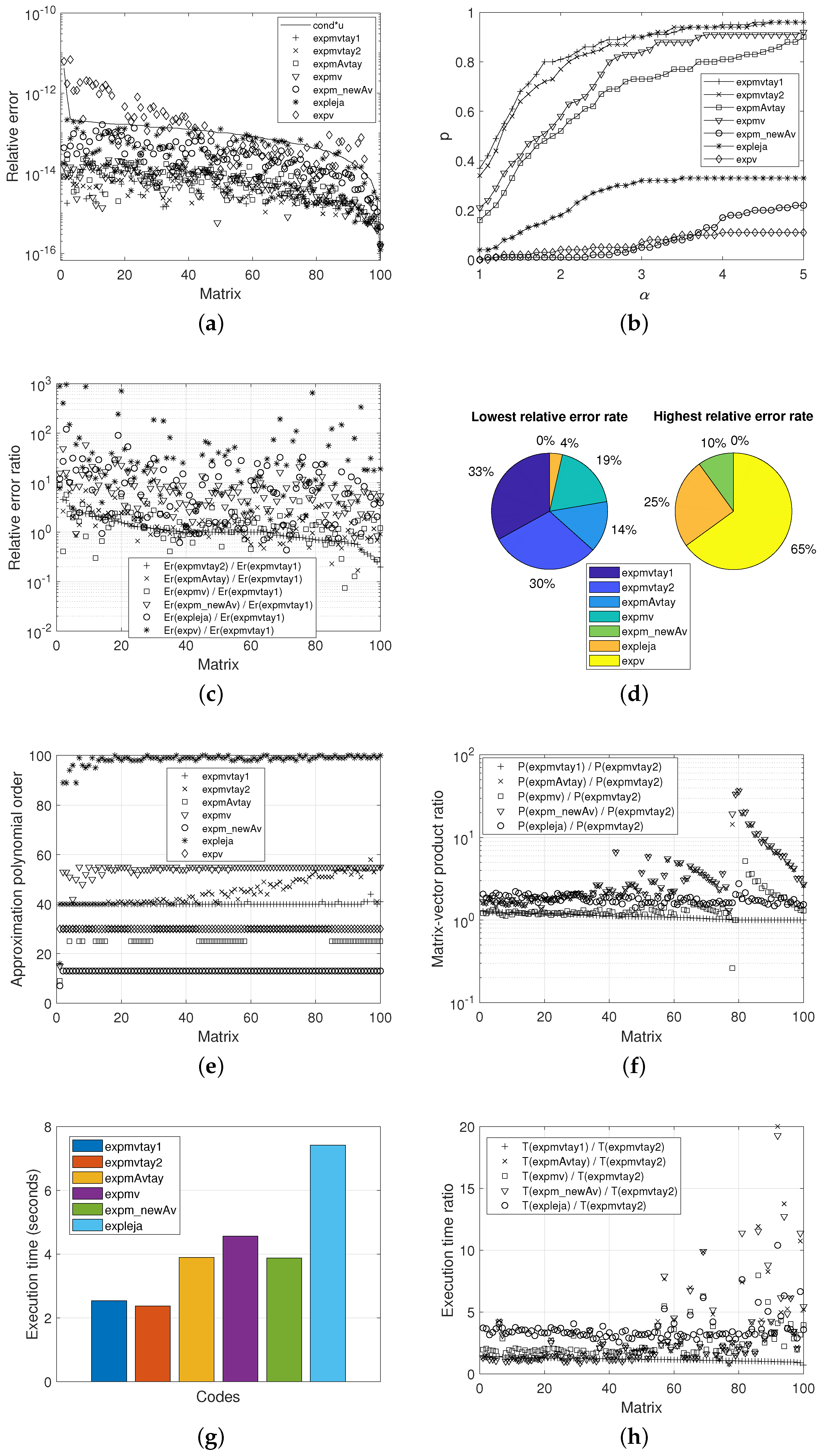
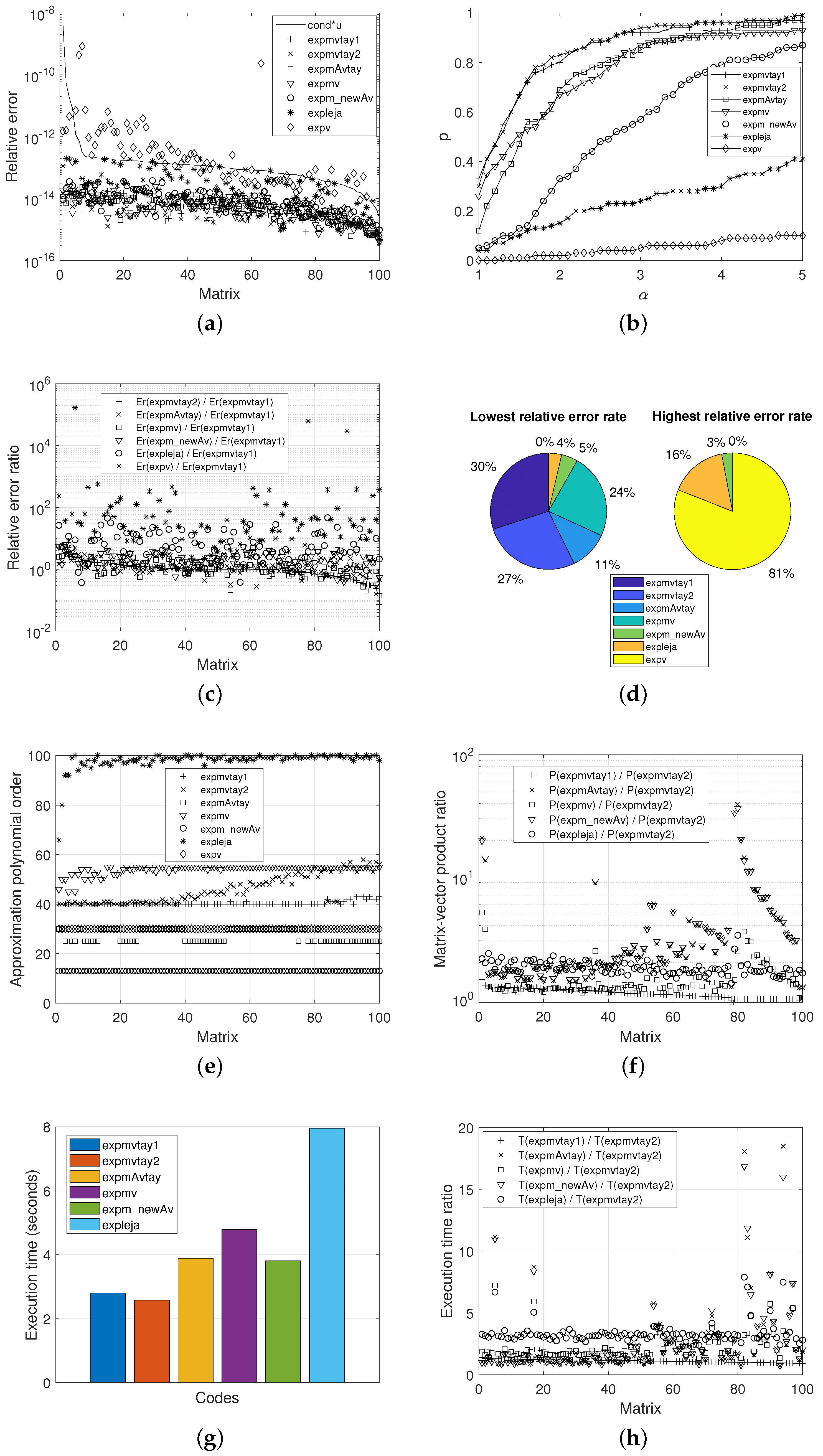
Figure 1,
Figure 2 and
Figure 3 show, respectively, the results of the numerical analyses carried out by means of each of the different codes in comparison with the three types of matrices considered. In more detail, these figures depict the normwise relative errors (a), the performance profiles (b), the ratios of normwise relative errors between
expmvtay1 and the rest of the implementations (c), the lowest and highest relative error rates (d), the polynomial orders and the Krylov subspace dimensions (e), the ratios of matrix–vector products between
expmvtay2 and the other codes (f), the response time (g), and the ratio of the execution time between
expmvtay2 and the remaining functions (h).
For each of the methods under evaluation, the normwise relative error
committed in the computation of the action of the exponential function of a matrix
A on a vector
v was calculated as follows:
where
denotes the exact solution and
represents the approximate one.
Figure 1a,
Figure 2a and
Figure 3a present the normwise relative error incurred by each of the seven codes under study. The solid line that appears in them plots the function
, where
(or
) means the condition number of the matrix exponential function ([
29], Chapter 3) for each matrix and
u represents the unit roundoff in IEEE double precision arithmetic. The matrices were ordered by decreasing value their condition number. It is well-known that the numerical stability of each method is exposed if its relative errors are positioned not far above this solid line, although it is always preferable that they are below. Consequently, these figures reveal that
expv is the code that most frequently presents relative errors above the
curve, being therefore the least numerically stable of all the codes analysed for the matrices used in the numerical tests. The rest of the codes can be said to offer high numerical stability.
The percentage of cases in which
expmvtay1 incurred in a normwise relative error less, equal or greater than the other codes is listed in
Table 2. As can be appreciated,
expmvtay1 always provided a higher percentage of improvement cases than the rest of its competitors, especially over
expv followed by
expm_newAv,
expleja, and, with very similar rates, by
expmAvtay and
expmv. On the other hand, the gain in accuracy by
expmvtay1 over
expmvtay2 is not noticeable, and it can be concluded that the latter will also offer a notable improvement in the reliability of the results compared to the rest of the methods.
In a very detailed way,
Table 3 collects the values corresponding to the minimum and maximum normwise relative error committed by all the functions for the three sets of matrices employed, as well as the mean, median, and standard deviation. While the minimum relative errors incurred by the codes are very similar, it is easy to observe how the maximum relative error and, consequently, the largest values in the mean, median, and standard deviation corresponded in general to
expv, which turned out to be the least reliable code, closely followed by
expleja and
expm_newAv. For all these metrics, the other methods, all based on the Taylor approximation, provided better values, analogous to each other.
Figure 1b,
Figure 2b and
Figure 3b, corresponding to the performance profiles, depict the percentage of matrices in each set, expressed in terms of one, for which the error committed by each method in comparison is less than or equal to the smallest relative error incurred by any of them multiplied by
. It is immediately noticeable that
expmvtay1 and
expmvtay2 achieved the highest probability values for the vast totality of the plots,
expmvtay1 showing a slightly highest accuracy than
expmvtay2 in
Figure 1b and similar in the other figures. The scores achieved by
expmAvtay and
expmv do not differ much from each other, and they are somewhat lower than those provided by the previous codes. Clearly,
expm_newAv,
expleja, and
expv exhibited the poorest results, with a significantly lower accuracy than the other codes.
These accuracy results are also confirmed by the next two types of illustrations.
Figure 1c,
Figure 2c and
Figure 3c reflect the ratio of the relative errors for any of the methods under study and
expmvtay1. Values of these ratios are decreasingly ordered and exposed according to the quotient
. Most of these values are greater than or equal to 1, showing once again the overall superiority of
expmvtay1, and correspondingly of
expmvtay2, over the other functions.
As a pie chart, and for each of the sets,
Figure 1d,
Figure 2d and
Figure 3d show the percentage of matrices in which each method resulted in the lowest or highest relative error. According to the values therein, for Sets 1 and 2,
expmvtay1 and
expmvtay2 gave rise to the lowest errors on a highest percentage of occasions. Notwithstanding, for Set 3, these percentages were almost equally distributed among
expmvtay1,
expmvtay2,
expmAvtay, and
expmv. If our attention is now turned to the highest relative error rates,
expv gave place to the worst results in most cases, leading to values equal to 65% and 81% for Sets 1 and 2, respectively. For Set 3, this percentage dropped to 40%, followed in a 29% by
expleja and in a 24% by
expm_newAv.
Table 4 compares the minimum, maximum, mean, and median values of the tuple
m and
s, i.e., the order of the Taylor approximation polynomial and the value of the scaling parameter used by the first four methods. For the other codes, the parameter
m is not comparable as it represents the degree of the Padé approximants to the matrix exponential (
expm_newAv), the selected degree of interpolation (
expleja) or the dimension of the Krylov subspace employed (
expmv). Additionally,
s denotes the scaling value (
expm_newAv) or the scaling steps (
expleja), but it is not provided for
expv, because this code does not work with the scaling technique.
Regarding the mean values,
expmv needed the highest orders of approximation polynomials, followed by
expmvtay2,
expmvtay1, and
expmAvtay. The function
expv was always invoked using the default value of
m, which corresponded to 30. Concerning the value of
s, also in average terms,
expmAvtay always required the smallest values, while
expmvtay1, in the case of matrix Sets 1 and 2, or
expmv, in the case of Set 3, demanded the highest values. Alternatively,
Figure 1e,
Figure 2e and
Figure 3e graphically represent the values of
m required in the computation of each of the matrices that compose our test battery by the distinct methods.
In addition to the above analysis related to the accuracy of the results provided by all the codes, their computational costs have also been examined from the point of view of the number of matrix–vector products and the execution time invested by each of them. Thus,
Table 5 lists the total number of matrix–vector products carried out by the seven codes in the computation of the matrices of our three sets. As can be noted,
expmvtay2 performed the lowest number of products, followed by
expmvtay1. Then, following an increasing order in the number of operations involved,
expmv,
expleja,
expmAvtay, and
expm_newAv would be cited, exchanging the position of these last two codes for Set 3. By far, the largest number of products was carried out by
expv.
In a more detailed way,
Figure 1f,
Figure 2f and
Figure 3f show the ratio between the number of matrix–vector products required by
expmvtay1,
expmAvtay,
expmv,
expm_newAv, or
expleja and that needed by
expmvtay2 in the computation of the matrices of the test sets, decreasingly ordered according to the quotient P(
expmvtay1)/P(
expmvtay2). In order not to distort these figures and to better appreciate the rest of the results, the ratio with respect to
expv has not been considered, due to its excessively high number of products demanded. In the case of Sets 1 and 2, this factor reached values greater than or equal to one in the vast majority of the matrices. For Set 3, it took values belonging to the intervals [1.00, 1.19], [0.89, 43.45], [0.31, 8.93], [0.85, 35.97], and [0.25, 25.78], respectively, for
expmvtay1,
expmAvtay,
expmv,
expm_newAv, and
expleja.
It is convenient to clarify that expmAvtay computes matrix–vector products to obtain the most appropriate values of the polynomial order (m) and the value of the scaling (s), especially with regard to the estimation of the 1-norm of or operations, where A and B are square matrices and p is the power parameter. In addition, this function works out matrix products not only in the calculation of these mentioned values, but also in the evaluation of the Taylor approximation polynomial by means of the Paterson–Stockmeyer method. Something very similar could be said about expm_newAv, as matrix–vector products will be carried out by the function expm_new in the estimation of the 1-norm of power of matrices, and matrix products will be as well required when calculating the matrix exponential by means of Padé approximation. As a consequence, the computational cost of each matrix product for expmAvtay and expm_newAv was approximated as n matrix–vector products, where n represents the dimension of the square matrices involved.
On the other hand,
Table 6 reports the amount of time required by all the codes in comparison to complete its execution. As expected according to the matrix–vector products,
expmvtay2 spent the shortest times, closely followed by
expmvtay1. Exceedingly time-consuming resulted to be
expv, particularly for Sets 1 and 2. The execution time of
expv was more moderate in the case of Set 3, where the response times of
expmAvtay and
expm_newAv were also remarkable due to the explicit computation of the matrix exponential and its subsequent product by the vector.
Figure 1g,
Figure 2g and
Figure 3g display graphically these same values by means of bar charts. Again,
expv times have not been included so as not to distort the graphs.
Finally, in
Figure 1h,
Figure 2h and
Figure 3h, and always following a descending sequence in the quotient T(
expmvtay1)/T(
expmvtay2), the ratios of the computation times spent by
expmvtay1,
expmAvtay,
expmv,
expm_newAv, and
expleja versus
expmvtay2 in each matrix computation are plotted. In the specific case of
expmv, this ratio took values within the intervals [1.54, 7.96], [1.35, 7.23], and [0.42, 10.21], respectively, for the Sets 1 to 3. As can be easily noticed in the figures, the results corresponding to
expmAvtay and
expm_newAv were the highest ones for any set.


