Article

Minimizing Travel Time and Latency in Multi-Capacity Ride-Sharing Problems

Department of Mathematics and Computer Science, Eindhoven University of Technology, 5600 MB Eindhoven, The Netherlands
*
Author to whom correspondence should be addressed.
Algorithms 2022, 15(2), 30; https://doi.org/10.3390/a15020030
Submission received: 7 December 2021 / Revised: 8 January 2022 / Accepted: 14 January 2022 / Published: 18 January 2022
(This article belongs to the Collection Feature Paper in Algorithms and Complexity Theory)

Abstract

:
Motivated by applications in ride-sharing and truck-delivery, we study the problem of matching a number of requests and assigning them to cars. A number of cars are given, each of which consists of a location and a speed, and a number of requests are given, each of which consists of a pick-up location and a drop-off location. Serving a request means that a car must first visit the pick-up location of the request and then visit the drop-off location. Each car can only serve at most c requests. Each assignment can yield multiple different serving routes and corresponding serving times, and our goal was to serve the maximum number of requests with the minimum travel time (called CS s u m ) and to serve the maximum number of requests with the minimum total latency (called CS l a t ). In addition, we studied the special case where the pick-up and drop-off locations of a request coincide. Both problems CS s u m and CS l a t are APX-hard when c 2 . We propose an algorithm, called the transportation algorithm (TA), which is a ( 2 c 1 ) -approximation (resp. c-approximation) algorithm for CS s u m (resp. CS l a t ); these bounds are shown to be tight. We also considered the special case where each car serves exactly two requests, i.e., c = 2 . In addition to the TA, we investigated another algorithm, called the match-and-assign algorithm (MA). Moreover, we call the algorithm that outputs the best of the two solutions found by the TA and MA the CA. We show that the CA is a two-approximation (resp. 5 / 3 ) for CS s u m (resp. CS l a t ), and these ratios are better than the ratios of the individual algorithms, the TA and MA.

1. Introduction

In the multi-capacity ride-sharing problem, we are given a set of cars (or trucks) D, each car k D located at location d k , and a set of requests R, each request r R consisting of a source s r (pick-up location) and a destination t r (drop-off location). Travel times are given between each pair of locations. Each car k D has capacity c. Serving a request means that a car first visits the pick-up location of the request (customer or parcel) and then the drop-off location. Each car can serve multiple requests at the same time. This offers the opportunity to share rides, which may reduce the travel time or traffic congestion. This paper is concerned with two objectives when assigning the maximum number of requests ( min { | R | , c · | D | } requests): one is to assign requests to the cars such that each car serves at most c requests while minimizing the total travel time, and the other problem is to assign requests to the cars such that each car serves at most c requests while minimizing the total waiting time (called total latency) incurred by customers that have submitted the requests. We now provide more insight into these two objectives:
  • Minimize total travel time: In this problem, we considered assigning the maximum number of requests to cars, each with no more than c requests, to minimize the total travel time, which is the sum of the travel times a car drives to serve its requests. Viewed from the ride-sharing company or drivers, minimizing the total travel time is the most important, since it results in minimizing the costs while serving the maximum number of requests. Furthermore, it also results in the minimum pollution or emissions. A solution for a given instance is a collection of trips with the minimum total travel time where a car visits all locations of the requests assigned to that car, while visiting the pick-up location of a request before the corresponding drop-off location. We call the ride-sharing problem with the objective of minimizing the total travel time CS s u m and the special case of CS s u m where the pick-up and drop-off locations are identical for each request CS s u m , s = t ;
  • Minimize total latency: In this problem, we considered assigning the maximum number of requests to cars, each with no more than c requests, to minimize the total waiting time, which is the sum of the travel times needed for each individual request (customer or parcel) to arrive at the destination. Passengers or clients care about reaching their destinations as soon as possible. Here, the goal is to obtain a solution that is a collection of trips where the travel time summed over the individual requests is minimum. We call the ride-sharing problem with the objective of minimizing the total latency CS l a t and the special case of CS l a t where the pick-up and drop-off locations are identical for each request CS l a t , s = t .

1.1. Motivation

Many ride-sharing companies (see [1]) provide a service (carpooling, ride-sharing, etc.) where customers submit their requests and then wait for the company to assign them a car. Consider a large number of requests in a working day morning, each consisting of a pick-up and a drop-off location. The company has a number of available cars whose locations and capacity c are known. The value of capacity c can be seen as the capacity of each car over time, i.e., the number of requests a car can accommodate in a relevant period of time. This value may well differ from the instantaneous capacity of a car (say the number of seats), as a pair of requests served by the same car may not be served simultaneously as one request is dropped off before the other request is picked up. In order to achieve a balanced allocation of requests to cars, each car receives no more than c requests. The task then is to assign the maximum number requests to available cars with respect to the capacity constraint.
It is a fact, however, that in many practical situations, “each request is allowed to occupy at most two seats in a car” (see Uber [1]). A regular vehicle has 4–8 seats; thus, only a limited number of requests can be combined in a single vehicle; this can be modeled by taking c 4 .
Consider the application of our problem in the area of collective transport. For instance, the company TransVision [2] provides transport service for specific groups of people (patients, commuters, etc.), and they organize collective transport by collecting requests in a particular region of The Netherlands in advance, combine these requests, and assign them to some regular transport companies. To access their service, customers must make their request the evening before the day of the actual transport; the number of requests for a day often exceeds 5000. In this application, each server (car, bus, etc.) may pick up more than four requests during its working period; hence, a value of c > 4 can be appropriate.
We can capture the above scenarios by the following problem: There is a set of customers who have specified their pick-up locations and drop-off locations to the vehicle provider, and the provider has a set of cars (also with drivers) that have a specified location and capacity c. The task, in this paper, is to assign customers to vehicles without exceeding the vehicles’ capacities and plan a service route for each of the vehicles based on optimization criteria, either minimizing the total travel time in CS s u m or minimizing the total latency in CS l a t .
The problems CS s u m , s = t and CS l a t , s = t are natural special cases of CS s u m and CS l a t , respectively, and can be used to model situations where parcels have to be delivered to clients (whose location is known and fixed). For instance, one can imagine a retailer sending out trucks to satisfy clients’ demands where each truck is used to satisfy multiple clients.

1.2. Related Work

There is a growing amount of literature related to ride-sharing (see [3] for a survey). In a ride-sharing system, a number of cars are provided to serve requests from customers in a fixed period of time. Typically, there are four types of ride-sharing models: one-to-one, meaning that each car serves a single request at a time (see [4,5,6,7]); one-to-many, meaning that each car can serve multiple requests at the same time (see [8,9]); many-to-one, meaning that one request can be served consecutively by multiple cars ([10]); many-to-many, which is a combination of the previous two models ([11]). The ride-sharing problem is to match requests and cars while either minimizing the cost (see [8,9]) or maximizing the profit (see [5,6,7,10]). In this paper, we study a ride-sharing problem of the one-to-many type with the objective of minimizing the cost.
Different versions of ride-sharing problems have been studied. Alonso-Mora et al. [12] and Pavone et al. [13] estimated what fleet size is appropriate for a city considering the cost of cars, a maximum waiting time for a customer, and the extra expense of moving cars. Agatz et al. [14] studied the problem of assigning cars to customers in real-time to minimize the expected total delivery cost. For a dynamic ride-sharing problem, Stiglic et al. [15] analyzed and showed that a small increase in the flexibility of either the cars or the customers can significantly increase performance. Furthermore, Wang et al. [16] introduced the notion of the stability of a ride-sharing system, and they presented methods to establish stable or nearly stable solutions. Considering the online ride-sharing model, Ashlagi et al. [17] studied the problem of matching requests while they arrive one by one and each of them must be either matched to another request within a prespecified period of time or discarded. Each request can be matched at most once and yields a positive profit. To maximize the total profit while requests arrive in an adversarial model, they provided a randomized four-competitive algorithm. Lowalekar et al. [18] studied a special case of the online version of the ride-sharing problem, such that the vehicles have to return to their depot after serving a number of requests.  [19] designed algorithms for the online ride-sharing problem under both the adversarial model and the random arrival model.
Mori and Samaranayake [20] studied the ride-sharing problem with arbitrary capacity while relaxing the assumption of serving all requests. They used an LP-based randomized rounding algorithm to obtain a solution, such that the expected fraction of unassigned requests was at most 1 / e , while the total cost of serving assigned requests was no more than the optimal solution.
This paper deals with a setting where the maximum number of requests needs to be assigned to the cars such that each car serves no more than c requests while minimizing the total travel time ( CS s u m ) or minimizing the total waiting time ( CS l a t ). As far as we are aware, this particular ride-sharing problem has not been extensively studied, especially for the latency criterion, i.e.,  CS l a t . Notice that when c = 1 , the ride-sharing problems CS s u m and CS l a t become minimum weight assignment problems, and an optimal solution can be found in O ( | D | 3 ) (see, e.g., [21]). Bei and Zhang [9] considered CS s u m with c = 2 and gave a 2.5 -approximation algorithm for it. Luo and Spieksma [22] proposed approximation algorithms for four versions of the problem, while still assuming c = 2 . Here, we generalize the ride-sharing problem to a problem involving any arbitrary constant c 2 .
In fact, both CS s u m and CS l a t with c = 2 are a special case of the so-called two-to-one assignment problem (2-1-AP) investigated by Goossens et al. [23]. Given a set G of n green elements and a set R of 2 n red elements, we call a triple a set of three elements that consists of a single green element and two red elements. Each triple has a non-negative cost-efficient, and the goal of the 2-1-AP problem is to find a collection of triples such that each element is covered exactly once while minimizing the sum of the corresponding cost coefficients. In the context of our ride-sharing problem with c = 2 , the green elements represent the cars, and the red elements represent the requests. The arguments presented in [23] allowed us to conclude that both CS s u m and CS l a t are APX-hard, already for c = 2 .
For the special case of 2-1-AP where the cost of each triple ( i , j , k ) is defined as the sum of the three corresponding distances, i.e.,  cost ( i , j , k ) = d i j + d j k + d k i , where the distances d satisfy the triangle inequality, Goossens et al. [23] gave an algorithm with the approximation ratio of 4 / 3 . The definition of the cost coefficients in CS s u m , as well as in CS l a t differs from the above expression for c o s t ( i , j , k ) ; we refer to Section 4 for a precise definition.

1.3. Our Results

We formulated and analyzed an algorithm, called the transportation algorithm (TA), that outputs a feasible solution to each of the four problems described above. This transportation algorithm belongs to a type of heuristics, called hub heuristics, which have been analyzed in the context of the multi-index assignment and multi-index transportation problems (see [24,25]). We identified the worst-case ratios of the TA for the four problems and show them to be tight (see [26] for the appropriate terminology). An overview of these results is shown in Table 1, where “ * ” means that the corresponding worst-case ratio is tight.
For the case c = 2 , we propose a so-called match-and-assign algorithm, the MA. We also define an algorithm, the CA, that consists of outputting the better of the solutions found by the TA and MA. An overview of the results for c = 2 is shown in Table 2 (see also [22]). Notice that for CS s u m , s = t , CS l a t , and CS l a t , s = t , the worst-case ratio of the combined algorithm (CA) is strictly better than each of the two worst-case ratios of the individual algorithms f which CA is composed.
The paper is organized as follows. In Section 2, we give a precise problem description. In Section 3, we present the transportation algorithm (TA) and analyze its performance for both CS s u m and CS l a t . In Section 4, we consider the special case where each car serves exactly two requests. We propose the match-and-assign algorithm (MA) and analyze the performance of the MA and CA (the better solution of the MA and TA) for both CS s u m and CS l a t . Section 5 concludes the paper.

2. Preliminaries

Notation. Given a metric space on vertices V, where the travel time between vertices x 1 V and x 2 V is denoted by w ( x 1 , x 2 ) , note that the travel times w ( x 1 , x 2 ) for all x 1 , x 2 V are non-negative, symmetric, and satisfy the triangle inequality. Furthermore, we extended the notation of travel time between two locations to the travel time of a path: w ( x 1 , x 2 , , x k ) = i = 1 k 1 w ( x i , x i + 1 ) . In the ride-sharing problem, we are given n cars, denoted by D = { 1 , 2 , , n } , each car k consisting of its location d k V and m requests R = { r 1 , r 2 , , r m } , each r i consisting of a source (pick-up location) and destination (drop-off location) pair ( s i , t i ) V × V . Each car can serve at most c requests. We want to find an allocation:
M = { ( k , R k ) : k D , R k R , | R k | c , R 1 , R 2 , . . , R n are pairwise disjoint } ,
serving the maximum number of requests while minimizing the total travel time or minimizing the total latency. In the basic setting, we suppose m = c · n (see Section 3.3 for the case m < c · n and m > c · n ); thus, | R k | = c holds for all k D of any feasible solution. We now elaborate on these two objectives.
Minimizing total travel time: For each ( k , R k ) M ( k D ) where R k contains c requests, i.e.,  | R k | = c , we denote the minimum travel time of serving all requests in R k by cost ( k , R k ) , i.e., the minimum time (or distance) of visiting all locations { s i , t i | i R k } starting from d k where s i is visited before t i . The length of the shortest Hamiltonian path of visiting all locations { s i , t i | i R k } starting from s r ( r R k ) with s i visited before t i is denoted by SHP ( s r , R k ) . We view cost ( k , R k ) as consisting of two parts: one term w ( d k , s r ) expressing the travel time between d k and the first pick-up location s r and another term SHP ( s r , R k ) ( r R k ) capturing the minimum travel time of visiting all requests starting from s r . (It is true that, in general, the SHP is NP-hard; however, in our case, the parameter c is a small constant leading to instances of a SHP of bounded size.) The travel time needed to serve requests in R k ( k D ) is then given by:
cost ( k , R k ) = min r R k { w ( d k , s r ) + SHP ( s r , R k ) } .
We denote the travel time of an allocation M by:
cost ( M ) = ( k , R k ) M cost ( k , R k ) .
In CS s u m and CS s u m , s = t , the goal is to find an allocation M that minimizes cost ( M ) .
Minimizing total latency: Here, we focus on the waiting time as perceived by an individual customer, from the moment the car leaves his/her location until the moment the customer reaches his/her drop-off location. For each ( k , R k ) M ( k D ) where R k contains c requests, i.e.,  | R k | = c , we denote the minimum total waiting time of all requests in R k by wait ( k , R k ) , i.e., the sum of the times to reach all drop-off locations t r ( r R k ) following a path that visits all locations { s i , t i | i R k } starting from d k while s i is visited before t i . We view wait ( k , R k ) as consisting of two parts: one term c · w ( d k , s r ) expressing the waiting time between d k and the first pick-up location s r ; another term SHWP ( s r , R k ) capturing the sum of waiting times from the first pick-up location s r to every other drop-off location, minimized over all feasible ways of traveling through the locations in R k . The latency needed to serve requests in R k ( k D ) is then given by:
wait ( k , R k ) = min r R k { c · w ( d k , s r ) + SHWP ( s r , R k ) } .
We denote the latency of an allocation M by:
wait ( M ) = ( k , R k ) M wait ( k , R k ) .
Thus, in  CS l a t and CS l a t , s = t , the goal is to find an allocation M that minimizes wait ( M ) .
Another variant of the ride-sharing problem considering the latency objective is counted with respect to the pick-up location rather than the drop-off location in CS l a t . In this setting, the drop-off location clearly becomes irrelevant to the objective, and our approximation results for CS l a t , s = t become valid for this variant.

3. The Transportation Algorithm and Its Analysis

We describe the transportation algorithm in Section 3.1 and analyze its performance for CS s u m , CS s u m , s = t , CS l a t , and  CS l a t , s = t in Section 3.2.

3.1. The Transportation Algorithm

In this section, we present the transportation algorithm. The idea of the algorithm is to assign to each car k D c requests based only on the travel times between the car locations d k and the request locations s r , t r , thereby ignoring travel times between different request locations.
We implemented this idea by replacing each car k D by c virtual cars { γ 1 ( k ) , , γ c ( k ) } , resulting in car sets Γ = { γ 1 ( 1 ) , , γ c ( 1 ) , , γ 1 ( n ) , , γ c ( n ) } with | Γ | = c · n . Next, we assigned c · n requests to the c · n cars using a particular definition of the cost v 1 ( γ i ( k ) , r ) (or v 2 ( γ i ( k ) , r ) ) between a request r R and a car γ i ( k ) Γ :
v 1 ( γ i ( k ) , r ) = w ( d k , s r , t r ) + w ( t r , d k ) i f i < c w ( d k , s r , t r ) i f i = c .
v 2 ( γ i ( k ) , r ) = ( c i + 1 ) w ( d k , s r , t r ) + ( c i ) w ( t r , d k ) i f i < c w ( d k , s r , t r ) i f i = c .
Next, we introduce how to assign c · n requests to the c · n cars. As is showed in Algorithm 1.
Algorithm 1 Transportation algorithm ( TA ( v ) ).
1:
Construct a graph: Let G 1 ( Γ R , v 1 ) (resp. G 2 ( Γ R , v 2 ) ) be the complete bipartite graph with left vertex-set Γ , right vertex-set R, and edge weights v 1 ( γ i ( k ) , r ) (resp. v 2 ( γ i ( k ) , r ) ) for γ i ( k ) Γ and r R .
2:
Find a min-weight assignment: Find a minimum weight assignment M 1 (resp, M 2 ) in G 1 ( Γ R , v 1 ) (resp, G 2 ( Γ R , v 2 ) ) with weight v 1 ( M 1 ) (resp. v 2 ( M 2 ) ).
3:
Output: TA ( v 1 ) { ( k , { r 1 , , r c } ) : ( γ 1 ( k ) , r 1 ) , , ( γ c ( k ) , r c ) M 1 } .
TA ( v 2 ) { ( k , { r 1 , , r c } ) : ( γ 1 ( k ) , r 1 ) , , ( γ c ( k ) , r c ) M 2 } .
A solution is then found by letting car k D serve the requests assigned to virtual cars { γ 1 ( k ) , , γ c ( k ) } . Let R k = { r 1 , r 2 , , r c } ( k D ) denote the requests assigned to a car k, where request r i R k is assigned to γ i ( k ) .
In our algorithm, two minimum weight assignments based on these costs are found: M 1 with weight v 1 ( M 1 ) and  M 2 with weight v 2 ( M 2 ) . We use M 1 to construct a solution for CS s u m and  M 2 to construct a solution for CS l a t .
Observe that v 1 ( M 1 ) = ( γ i ( k ) , r ) M 1 v 1 ( γ i ( k ) , r ) . This amounts to a solution where each car k D travels according to the following path:
d k s r 1 t r 1 d k s r 2 t r 2 d k s r c t r c .
Notice that, due to the triangle inequality, the cost of such a path will not increase by “short-cutting” the path, i.e., by traveling from each t r i directly to s r i + 1 :
d k s r 1 t r 1 s r 2 t r 2 t r c 1 s r c t r c .
In fact, we use TA ( v 1 ) to denote this resulting solution found by the TA for CS s u m , with  cost ( TA ( v 1 ) ) denoting its cost.
We conclude:
cost ( TA ( v 1 ) ) v 1 ( M 1 ) .
A similar observation can be made with respect to M 2 . The quantity v 2 ( M 2 ) collects the waiting time of all requests by following, for each car k D , the path:
d k s r 1 t r 1 d k s r 2 t r 2 d k s r c t r c .
As argued above, shortcutting gives us then a feasible solution for an instance of CS l a t we denote by TA ( v 2 ) with cost wait ( TA ( v 2 ) ) . We have:
wait ( TA ( v 2 ) ) v 2 ( M 2 ) .
Recall that our problem does not force the driver to return to the original position. This implies that the cost of a driver when serving a set of request R k does not include the time from the last drop-off location to the driver’s original location. This explains why in the expression for v 1 ( M 1 ) (also, v 2 ( M 2 ) ), we can subtract the corresponding travel time from the total travel time. We now give two lemmas concerning v 1 ( M 1 ) (which we need to prove Theorem 1) and two more lemmas concerning v 2 ( M 2 ) (which we need to prove Theorem 2).
Lemma 1.
For any c 2 , we have:
v 1 ( M 1 ) = ( k , R k ) TA ( v 1 ) r R k w ( d k , s r , t r , d k ) max r R k w ( d k , t r ) .
Proof. 
We claim that v 1 ( M 1 ) is minimized if and only if, for each car k D and ( γ c ( k ) , r c ) M 1 , r c = arg max r R k w ( d k , t r ) . If this claim holds, then based on the definition of the cost v 1 ( · , · ) , we have v 1 ( k , R k ) = r R k w ( d k , s r , t r , d k ) w ( d k , t r c ) = r R k w ( d k , s r , t r , d k ) max r R k w ( d k , t r ) , and thus:
v 1 ( M 1 ) = ( k , R k ) TA ( v 1 ) r R k w ( d k , s r , t r , d k ) max r R k w ( d k , t r ) .
It remains to prove the claim. Consider any R k = { r 1 , r 2 , , r c } for car k D . We prove that v 1 ( M 1 ) is minimized if and only if w ( d k , t r c ) w ( d k , t r x ) for all r x R k .
Necessary condition: Since v 1 ( k , R k ) is minimized, we have w ( d k , s r x , t r x ) + w ( d k , t r x ) + w ( d k , s r c , t r c ) w ( d k , s r c , t r c ) + w ( d k , t r c ) + w ( d k , s r x , t r x ) based on the definition of v 1 (see Equation (5)), then w ( d k , t r x ) w ( d k , t r c ) holds.
Sufficient condition: Since w ( d k , t r c ) w ( d k , t r x ) , then w ( d k , s r c , t r c ) + w ( d k , t r c ) + w ( d k , s r x , t r x ) w ( d k , s r x , t r x ) + w ( d k , t r x ) + w ( d k , s r c , t r c ) , and that means v 1 ( M 1 ) is minimized as r c = arg max r R k w ( d k , t r ) .    □
From the above lemma and the fact that M 1 is a minimum weight assignment in G 1 ( Γ R , v 1 ) , we have the following lemma:
Lemma 2.
For c 2 and for each allocation M, we have:
v 1 ( M 1 ) ( k , R k ) M r R k w ( d k , s r , t r , d k ) max r R k w ( d k , t r ) .
We now provide two lemmas concerning v 2 ( M 2 ) . In the statement of these lemmas, we index the requests such that, for each k D , R k = { r 1 , r 2 , , r c } .
Lemma 3.
For any c 2 , for each car k D and r x , r y R k with x < y , w ( d k , s r x , t r x ) + w ( d k , t r x ) w ( d k , s r y , t r y ) + w ( d k , t r y ) .
Proof. 
We claim that v 2 ( M 2 ) is minimized if and only if for each car k D and r x , r y R k = { r 1 , r 2 , , r c } with x < y , w ( d k , s r x , t r x ) + w ( d k , t r x ) w ( d k , s r y , t r y ) + w ( d k , t r y ) . Consider r x , r y R k = { r 1 , r 2 , , r c } with x < y for car k D . We prove that v 2 ( M 2 ) is minimized if and only if w ( d k , s r x , t r x ) + w ( d k , t r x ) w ( d k , s r y , t r y ) + w ( d k , t r y ) .
Necessary condition: Since v 2 ( M 2 ) is minimized, based on definition of cost v 2 ( · , · ) , we have:
( c x + 1 ) w ( d k , s r x , t r x ) + ( c x ) w ( t r x , d k ) + ( c y + 1 ) w ( d k , s r y , t r y ) + ( c y ) w ( t r y , d k ) ( c x + 1 ) w ( d k , s r y , t r y ) + ( c x ) w ( t r y , d k ) + ( c y + 1 ) w ( d k , s r x , t r x ) + ( c y ) w ( t r x , d k ) .
( y x ) ( w ( d k , s r x , t r x ) + w ( d k , t r x ) ) ( y x ) ( w ( d k , s r y , t r y ) + w ( d k , t r y ) )
Thus, w ( d k , s r x , t r x ) + w ( d k , t r x ) w ( d k , s r y , t r y ) + w ( d k , t r y ) , since x < y .
Sufficient condition: According to the above statement, the condition w ( d k , s r x , t r x ) + w ( d k , t r x ) w ( d k , s r y , t r y ) + w ( d k , t r y ) implies that v 2 ( M 2 ) is minimized.    □
Since M 2 is a minimum weight assignment in G 2 ( Γ R , v 2 ) , we have the following lemma:
Lemma 4.
For c 2 and for each allocation M, we have:
v 2 ( M 2 ) ( k , R k ) M i = 1 c ( c i + 1 ) · w ( d k , s r i , t r i ) + ( c i ) · w ( d k , t r i ) .

3.2. Approximation Analysis of the TA

Let us denote an optimal allocation in CS s u m by M * = { ( k , R k * ) : k D } . Let M R * = { R k * : ( k , R k * ) M * } denote the collection of c-tuples of requests in an optimal solution M * . We now establish the worst-case ratios of the TA ( v 1 ) for CS s u m and CS s u m , s = t .
Theorem 1.
The TA ( v 1 ) is a ( 2 c 1 ) -approximation algorithm for CS s u m . Moreover, there exists an instance I of CS s u m , s = t for which cost ( TA ( v 1 ) ( I ) ) = ( 2 c 1 ) · cost ( M * ( I ) ) .
Proof. 
cost ( TA ( v 1 ) ) v 1 ( M 1 )
( k , R k * ) M * r R k * w ( d k , s r , t r , d k ) max r R k * w ( d k , t r )
= ( k , R k * ) M * r R k * w ( d k , s r , t r ) + r R k * w ( t r , d k ) max r R k * w ( d k , t r )
( k , R k * ) M * ( 2 c 1 ) cost ( k , R k * )
= ( 2 c 1 ) cost ( M * )
We now comment on the validity of the inequalities above. Inequality (9) follows from applying Inequality (7), and Inequality (10) follows from Lemma 2. The final Inequality (12) follows from the fact that for any r R k * , w ( d k , t r ) w ( d k , s r , t r ) cost ( k , R k * ) .
To see that the bound 2 c 1 is tight even for CS s u m , s = t , consider the instance I depicted in Figure 1. This instance has c cars D = { k 1 , k 2 , , k c } with car locations { d 1 , d 2 , , d c } and c 2 requests R = { 1 , 2 , , c 2 } with locations { s 1 , s 2 , , s c 2 } (the pick-up and drop-off locations are identical for each request). Locations corresponding to distinct vertices in Figure 1 are at Travel Time 1. Observe that an optimal solution is M * ( I ) = { ( k 1 , { 1 , 2 , , c } ) , ( k 2 , { c + 1 , c + 2 , , 2 c } ) , , ( k c , { c ( c 1 ) + 1 , c ( c 1 ) + 2 , , c 2 } ) } with cost( M * ( I ) ) = c .
Let us now analyze the performance of TA ( v 1 ) on instance I. Notice that TA ( v 1 ) may assign requests { i , c + i , , ( c 1 ) c + i } to car k i . In that case, the total cost of TA ( v 1 ) is c ( 2 ( c 1 ) + 1 ) ) = c ( 2 c 1 ) , showing tightness.    □
We proceed by establishing the worst-case ratios of the TA ( v 2 ) for CS l a t and CS l a t , s = t . Again, we assume that an optimal solution to CS l a t is denoted by M * , and the collection of c-tuples of requests in M * is denoted by M R * = { R k * : ( k , R k * ) M * } . In the following theorem, we index the requests such that, for each k D , R k * = { r 1 , r 2 , , r c } .
Theorem 2.
The TA ( v 2 ) is a c-approximation algorithm for CS l a t . Moreover, there exists an instance I of CS l a t , s = t for which wait ( TA ( v 2 ) ( I ) ) = c · wait ( M * ( I ) ) .
Proof. 
wait ( TA ( v 1 ) ) v 2 ( M 2 )
( k , R k ) M * i = 1 c ( c i + 1 ) · w ( d k , s r i , t r i ) + ( c i ) · w ( d k , t r i )
= ( k , R k * ) M * i = 1 c c · w ( d k , s r i , t r i ) ( i 1 ) · w ( d k , s r i , t r i ) + ( c i ) · w ( d k , t r i )
( k , R k * ) M * i = 1 c c · w ( d k , s r i , t r i )
( k , R k * ) M * c · wait ( k , R k * )
= c · wait ( M * )
We now comment on the validity of the inequalities above. Inequality (14) follows from applying Inequality (8), and Inequality (15) follows from Lemma 4. Inequality (17) follows from (we prove it later):
i = 1 c ( i 1 ) · w ( d k , s r i , t r i ) + ( c i ) · w ( d k , t r i ) 0 .
The final Inequality (18) follows from the fact that i = 1 c w ( d k , s r , t r ) wait ( k , R k * ) .
Notice that:
i = 1 c ( i 1 ) · w ( d k , s r i , t r i ) + ( c i ) · w ( d k , t r i ) i < c + 1 2 ( c 2 i + 1 ) · w ( d k , t r i ) i c + 1 2 ( 2 i c 1 ) · w ( d k , s r i , t r i ) = i < c + 1 2 ( c 2 i + 1 ) · w ( d k , t r i ) ( 2 ( c + 1 i ) c 1 ) · w ( d k , s r c + 1 i , t r c + 1 i ) 0
where the first inequality follows from the triangle inequality; the second inequality follows from w ( d k , t r x ) w ( d k , s r y , t r y ) for all r x , r y R k * with x < y since w ( d k , s r x , t r x ) + w ( d k , t r x ) w ( d k , s r y , t r y ) + w ( d k , t r y ) by Lemma 3.
To see that the bound c is tight even for CS l a t , s = t , consider the instance depicted in Figure 1. Observe that an optimal solution is M * ( I ) = { ( k 1 , { 1 , 2 , , c } ) , ( k 2 , { c + 1 , c + 2 , , 2 c } ) , , ( k c , { c ( c 1 ) + 1 , c ( c 1 ) + 2 , , c 2 } ) } with wait ( M * ( I ) ) = c 2 . Let us now analyze the performance of TA ( v 2 ) on instance I. TA ( v 2 ) may assign requests { i , c + i , , ( c 1 ) c + i } to car k i . In that case, the total waiting time of TA ( v 2 ) is c · ( 1 + 3 + + ( 2 ( i 1 ) + 1 ) + + 2 ( c 1 ) + 1 ) ) = c ( c · ( 1 + 2 c 1 ) / 2 ) = c 3 , showing tightness.    □

3.3. Discussion

Clearly, the TA is a polynomial-time algorithm, and it is easy to implement; moreover, it can be generalized to handle a variety of situations. We now list three situations and briefly comment on the corresponding worst-case behavior:
  • Ride-sharing with car-dependent speeds or relatedride-sharing. In this situation, the cars have speed p 1 , p 2 , , p n . The travel time of serving requests in R k is denoted by cost ( k , R k ) / p k , and the total travel time of an allocation M is denoted by ( k , R k ) M cost ( k , R k ) / p k . Analogously, the total latency of an allocation M is denoted by ( k , R k ) M wait ( k , R k ) / p k . Without going into the details, we point out that the TA can be modified by appropriately redefining v 1 ( k , r ) and v 2 ( k , r ) in terms of the cost above; we claim that the corresponding worst-case ratios of TA as shown in Table 1 remain unchanged;
  • Ride-sharing with car-dependent speeds or relatedride-sharing. In this situation, the cars have speed p 1 , p 2 , , p n . The travel time of serving requests in R k is denoted by cost ( k , R k ) / p k , and the total travel time of an allocation M is denoted by ( k , R k ) M cost ( k , R k ) / p k . Analogously, the total latency of an allocation M is denoted by ( k , R k ) M wait ( k , R k ) / p k . Without going into the details, we point out that the TA can be modified by appropriately redefining v 1 ( k , r ) and v 2 ( k , r ) in terms of the cost above; we claim that the corresponding worst-case ratios of TA as shown in Table 1 remain unchanged;
  • Car redundancy: c · n > m . In this situation, our problem is to find an allocation that serves all requests with the minimum total cost (total travel time or total latency). Clearly, some cars may serve less than c requests, or even do not serve a request. To apply TA for this situation, we need to add a number of requests to fill the shortage of requests, without affecting the total travel time or latency. We created an instance of our problem by adding a number of dummy requests R d with | R d | = c · n m , where the travel time between a request in R d and a car in D is zero, i.e.,  v 1 ( γ i ( k ) , r ) = 0 and v 2 ( γ i ( k ) , r ) = 0 for all i [ c ] , k D , r R d . Since the cost of assigning dummy requests is zero in any feasible solution, removing dummy requests of a solution for the newly created instance with c · n = | R | will give us a solution to the original instance;
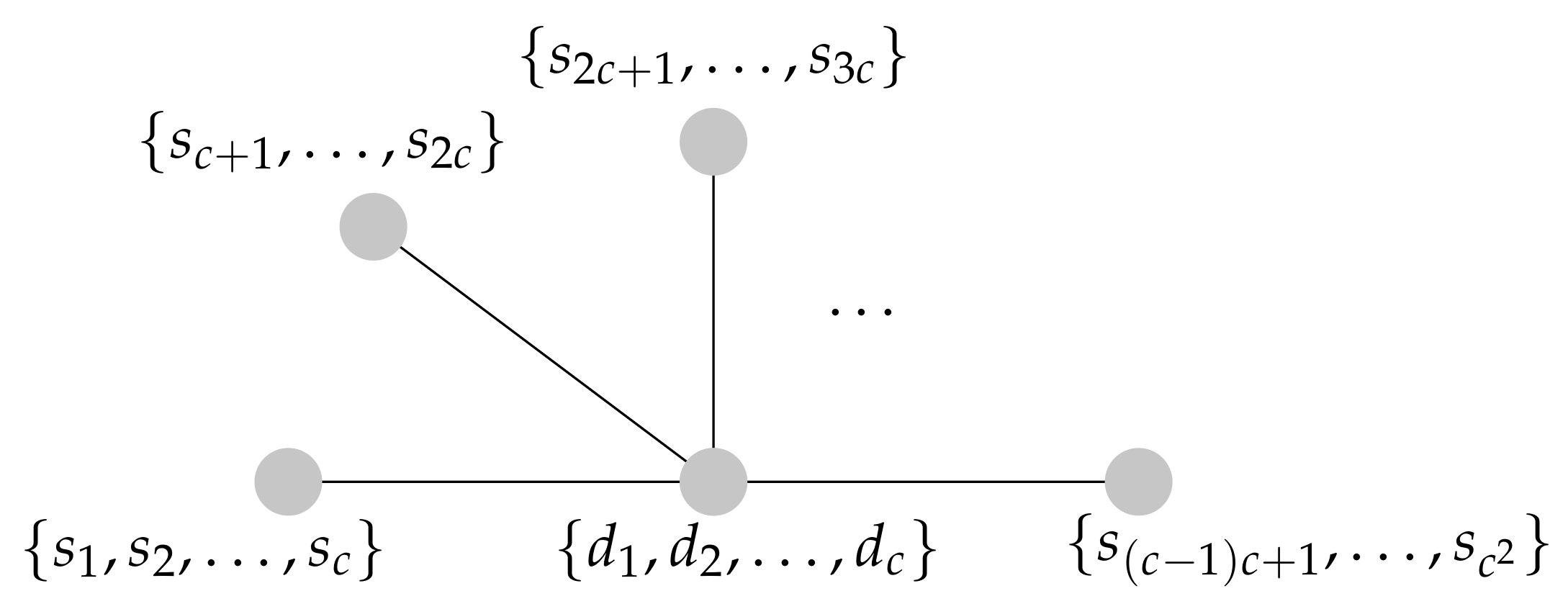
  • Car deficiency: c · n < m . In this situation, our problem is to find an allocation that serves the maximum number of requests ( c · n requests) with the minimum total cost (total travel time or total latency). It follows that some requests will not be served. To apply the TA for this situation, we created an instance of our problem by adding a number of dummy cars D d with | D d | = m n · c , where the travel time between a car in D d and a request in R is H (H is a sufficiently large number), i.e.,  v 1 ( k , r ) = H and v 2 ( k , r ) = H for all k D d , r R . Removing dummy cars (and their corresponding requests) gives us a solution to the original instance. Since we found an assignment with the minimum total weight and we removed the set of requests assigned to the dummy cars, we claim that the TA selected c · n requests with the minimum total weight. In fact, the proofs in Section 3.1 imply that the TA ( v 1 ) is a ( 2 c 1 ) -approximation algorithm for CS s u m and the  TA ( v 2 ) is a c-approximation algorithm for CS l a t .

4. The Case c = 2 : Algorithms and Their Analysis

In this section, we consider the ride-sharing problems CS s u m , CS s u m , s = t , CS l a t , and CS l a t , s = t with capacity c = 2 and each car serving exactly two requests, i.e.,  m = 2 n (see [22]). In Section 4.1, we propose and analyze the match-and-assign algorithm ( MA ). Next, in Section 4.2, we analyze the combined algorithm ( CA ), i.e., the better of the two algorithms, the MA and TA .
For convenience, we explicitly write the quantity SHP ( s i , { i , j } ) in CS s u m by a parameter u i j as follows:
u i j min { w ( s i , s j , t i , t j ) , w ( s i , s j , t j , t i ) , w ( s i , t i , s j , t j ) } f o r e a c h i , j R × R , i j .
Notice that the u i j ’s are not necessarily symmetric. Obviously, u i j w ( s i , s j ) and u j i w ( s i , s j ) . For  CS s u m , s = t , we have u i j = u j i w ( s i , s j ) .
The travel time needed to serve requests in R k = { i , j } ( k D ) is then given by:
cost ( k , { i , j } ) = min { w ( d k , s i ) + u i j , w ( d k , s j ) + u j i } .
For convenience, we also explicitly write the quantity SHWP ( s i , { i , j } ) in CS s u m by a parameter μ i j as follows:
μ i j min { w ( s i , s j , t i ) + w ( s i , s j , t i , t j ) , w ( s i , s j , t j ) + w ( s i , s j , t j , t i ) , w ( s i , t i ) + w ( s i , t i , s j , t j ) } f o r e a c h i , j R × R , i j .
Notice that the μ i j ’s are not necessarily symmetric. For  CS l a t , s = t , we have μ i j = μ j i w ( s i , s j ) .
The latency needed to serve requests in R k = { i , j } ( k D ) is then given by:
wait ( k , { i , j } ) = min { 2 w ( d k , s i ) + μ i j , 2 w ( d k , s j ) + μ j i } .

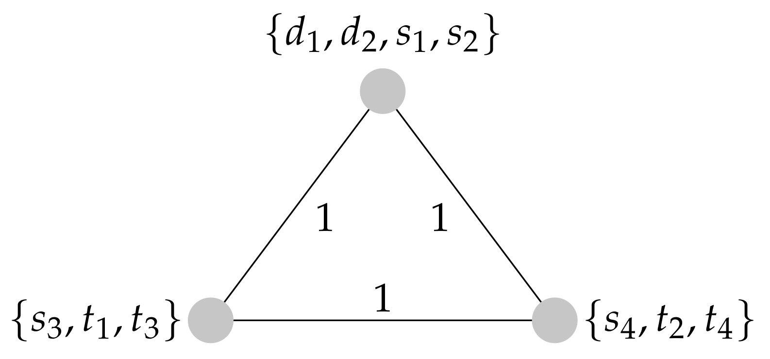
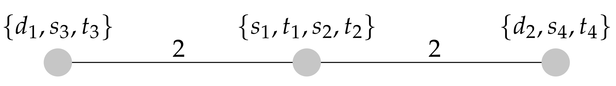
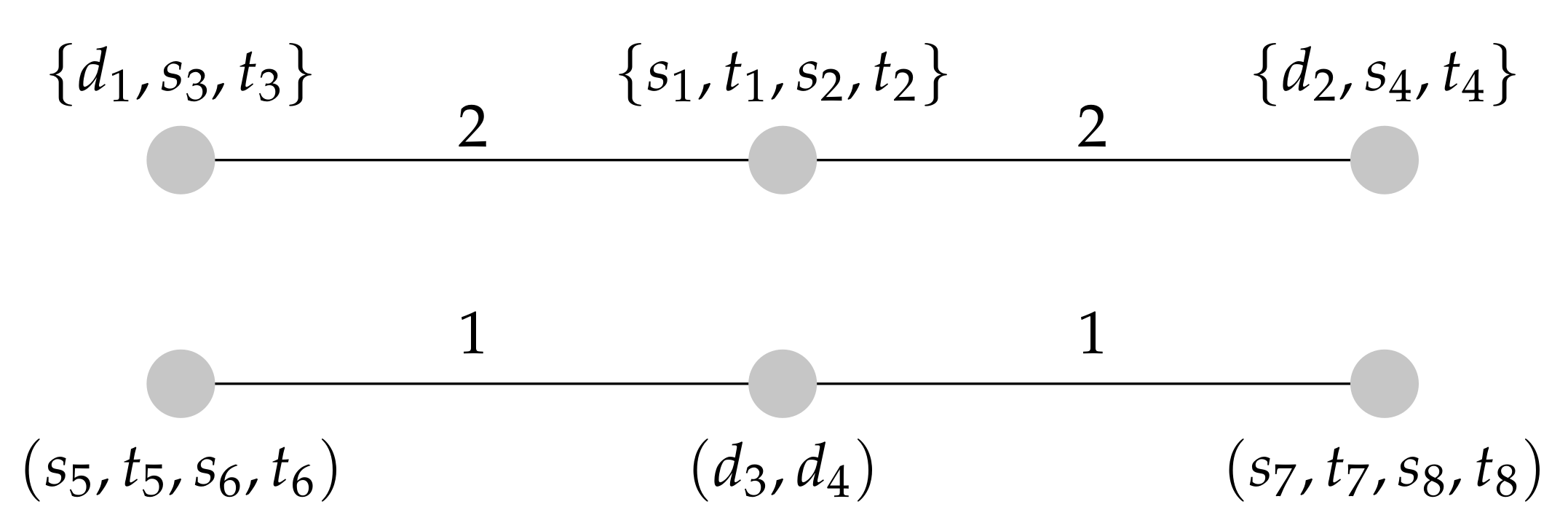
4.1. The Match-and-Assign Algorithm and Its Analysis

We came up with a match-and-assign algorithm, the MA ( α , v ) , the idea being that, first, requests are matched into request pairs, after which the request pairs are assigned to the cars. Finding request pairs is performed by using a carefully chosen time v 3 ( { i , j } ) between a pair of requests { i , j } , as well as a travel time v 4 ( k , { i , j } ) between each request pair { i , j } and a car k D :
v 3 ( { i , j } ) v i j + v j i 2 , v { u , μ } .
v 4 ( k , { i , j } ) min { α w ( d k , s i ) + v i j v j i 2 , α w ( d k , s j ) v i j v j i 2 } , α { 1 , 2 } , v { u , μ } .
Now, we introduce the match-and-assign Algorithm 2.
The resulting quantity is v 3 ( M 3 ) + v 4 ( M 4 ) ; we now prove two lemmas concerning this quantity, which will be of use in the approximation analysis.
Algorithm 2 Match-and-assign algorithm ( MA ( α , v ) ).
1:
Matching step:
  • Construct a graph: Let G 3 ( R , v 3 ) be the complete weighted graph where an edge between vertex i R and vertex j R has weight v 3 ( { i , j } ) ;
  • Find a min-weight matching: Find a minimum weight perfect matching M 3 in G 3 ( R , v 3 ) with weight v 3 ( M 3 ) .
2:
Assignment step:
  • Construct a graph: Let G 4 ( D M 3 , v 4 ) be the complete bipartite graph with left vertex-set D, right vertex-set M 3 , and edges with weight v 4 ( k , { i , j } ) for k D , and  { i , j } M 3 ;
  • Find a min-weight assignment: Find a minimum weight assignment M 4 in G 4 ( D M 3 , v 4 ) with weight v 4 ( M 4 ) .
3:
Output: MA = M 4 .
Lemma 5.
For each α { 1 , 2 } and v { u , μ } , we have:
v 3 ( M 3 ) + v 4 ( M 4 ) = ( k , { i , j } ) M 4 min { α w ( d k , s i ) + v i j , α w ( d k , s j ) + v j i } .
Proof. 
Without loss of generality, for any { i , j } M 3 , suppose v i j v j i 0 (the other case is symmetric).
v 3 ( M 3 ) + v 4 ( M 4 ) = { i , j } M 3 v i j + v j i 2 + = ( k , { i , j } ) M 4 min { α w ( d k , s i ) + v i j v j i 2 , α w ( d k , s j ) v i j v j i 2 } = ( k , { i , j } ) M 4 min { α w ( d k , s i ) + v i j , α w ( d k , s j ) + v j i } .
The first equality follows from the definition of v 3 and v 4 (see Equations (24) and (25)). □
Lemma 6.
For α { 1 , 2 } , v { u , μ } , and for each allocation M, we have:
v 3 ( M 3 ) + v 4 ( M 2 ) ( k , { i , j } ) M α w ( d k , s i ) + α w ( d k , s j ) + v i j + v j i 2 .
Proof. 
For an allocation M, let M R = { R k : ( k , R k ) M } . Observe that:
v 3 ( M 3 ) { i , j } M R v i j + v j i 2 ,
since M 3 is a minimum weight perfect matching in G 3 ( R , v 3 ) .
We claim that:
v 4 ( M 4 ) ( k , { i , j } ) M α w ( d k , s i ) + α w ( d k , s j ) 2 .
When summing (26) and (27), the lemma follows.
Hence, it remains to prove (27). Consider an allocation M, and consider the matching M 3 found in the first step of the MA . Based on M and M 3 , we construct the graph G = ( R D , M 1 { ( { i , k } , { j , k } ) : ( k , { i , j } ) M } ) . Note that every vertex in graph G has degree two. Thus, we can partition G into a set of disjoint cycles called C; each cycle c C can be written as c = ( i 1 , j 1 , k 1 , i 2 , j 2 , k 2 , , k h , i 1 ) , where { i s , j s } M 3 , ( k s , { j s , i s + 1 } ) M for 1 s < h and ( k h , { j h , i 1 } ) M . Consider now, for each cycle c C , the following two assignments called M c and M r c :
  • M c = { ( { i 1 , j 1 } , k 1 ) , ( { i 2 , j 2 } , k 2 ) , , ( { i h , j h } , k h ) } ,
  • M r c = { ( k 1 , { i 2 , j 2 } ) , ( k 2 , { i 3 , j 3 } ) , , ( k h , { i 1 , j 1 } ) } .
Obviously, both M c C M c and M r c C M r c are a feasible assignment in G 4 = ( D M 3 , v 4 ) . Given the definition of v 4 ( k , { i , j } ) (see Equation (25)), we derive for each pair of requests { i , j } and two cars a , b : v 4 ( a , { i , j } ) + v 2 ( b , { i , j } ) α w ( d a , s i ) + v i j v j i 2 + α w ( d b , s j ) v i j v j i 2 = α ( w ( d a , s i ) + w ( d b , s j ) ) . Similarly, it follows that: v 4 ( a , { i , j } ) + v 4 ( b , { i , j } ) α ( w ( d a , s j ) + w ( d b , s i ) ) . Thus, for each c C :
( k , { i , j } ) M c v 4 ( k , { i , j } ) + ( k , { i , j } ) M r c v 4 ( k , { i , j } ) { i , k } , { j , k } c ( k , { i , j } ) M α ( w ( d k , s i ) + w ( d k , s j ) ) .
Note that M 4 is a minimum weight assignment in G 4 = ( D M 3 , v 4 ) , and both M and M r are a feasible assignment in G 4 = ( D M 3 , v 4 ) . Thus:
v 4 ( M 4 ) c C min { v 4 ( M c ) , v 4 ( M r c ) } 1 2 c C ( k , { i , j } ) M c v 4 ( k , { i , j } ) + ( k , { i , j } ) M r c v 4 ( k , { i , j } ) ( k , { i , j } ) M α w ( d k , s i ) + α w ( d k , s j ) 2 .
The last inequality follows from (28), and hence, (27) is proven. □
Lemma 7.
For any two requests i and j, we have:
max { u i j , u j i } min { u i j , u j i } w ( s i , s j ) ;
and:
u i j 2 u j i .
Without loss of generality, suppose u i j u j i , u i j w ( s i , s j ) + u j i . Since w ( s i , s j ) min { u i j , u j i } , we have u i j 2 u j i for any two requests i and j.
Theorem 3.
The MA ( 1 , u ) is a two-approximation algorithm for CS s u m . Moreover, there exists an instance I for which cost ( MA ( I ) ) = 2 cost ( M * ( I ) ) .
Proof. 
We assume w.l.o.g. that, for each ( k , { i , j } ) M * , cost ( k , { i , j } ) = w ( d k , s i ) + u i j . We have:
cost ( MA ( 1 , u ) ) = ( k , { i , j } ) MA min { w ( d k , s i ) + u i j , w ( d k , s j ) + u j i }
= v 3 ( M 3 ) + v 4 ( M 4 )
( k , { i , j } ) M * w ( d k , s i ) + w ( d k , s j ) + u i j + u j i 2
( k , { i , j } ) M * 2 w ( d k , s i ) + w ( s i , s j ) + 3 u i j 2
1 2 ( k , { i , j } ) M * ( 2 w ( d k , s i ) + 4 u i j )
1 2 ( k , { i , j } ) M * 4 cost ( k , { i , j } )
= 2 cost ( M * ) .
Equation (29) follows from (2) and (21). Equation (30) follows from Lemma 5. Inequality (31) follows from Lemma 6. Inequality (32) follows from the triangle inequality, and u j i 2 u i j for each request pair { i , j } R 2 based on Lemma 7. Inequality (33) follows from w ( s i , s j ) u i j . Notice that cost ( MA ( I ) ) 2 cost ( M * ( I ) ) is actually tight by the instance depicted in Figure 2. □
Theorem 4.
The MA ( 1 , u ) is a 3 / 2 -approximation algorithm for CS s u m , s = t . Moreover, there exists an instance I for which cost ( MA ( I ) ) = 3 / 2 cost ( M * ( I ) ) .
Proof. 
cost ( MA ( 1 , u ) ) = ( k , { i , j } ) MA min { w ( d k , s i ) + u i j , w ( d k , s j ) + u j i }
( k , { i , j } ) M * w ( s i , s j ) + w ( d k , s i ) + w ( d k , s j ) 2
( k , { i , j } ) M * 3 / 2 cost ( k , { i , j } )
3 / 2 cost ( M * )
Equation (36) follows from (20). Inequality (37) follows from Lemma 5 and 6, and u i j = u j i = w ( s i , s j ) .
To see that the equality may hold in cost ( MA ( I ) ) 3 / 2 cost ( M * ( I ) ) , consider the subgraph induced by the nodes ( d 1 , s 3 ) , ( s 1 , s 2 ) , and ( d 2 , s 4 ) in Figure 3 with cars { k 1 , k 2 } and requests { 1 , 2 , 3 , 4 } . Observe that an optimal solution is { ( k 1 , { 1 , 3 } ) , ( k 2 , { 2 , 4 } ) } with cost ( M * ( I ) ) = 2 . Note that MR * = { { 1 , 3 } , { 2 , 4 } } . Let us now analyze the performance of MA ( 1 , u ) on this instance. Based on the u values as defined in (20), MA ( 1 , u ) can find, in the first step, matching M 3 = { { 1 , 2 } , { 3 , 4 } } because v 3 ( M 3 ) = v 3 ( MR * ) = 2 . Then, no matter how the second step assigns the request pairs to cars, the total waiting time of MA ( 1 , u ) will be three. □
Theorem 5.
The MA ( 2 , μ ) is a two-approximation algorithm for CS l a t . Moreover, there exists an instance I of CS l a t , s = t for which wait ( MA ( I ) ) = 2 wait ( M * ( I ) ) .
Proof. 
wait ( MA ( 2 , μ ) ) = ( k , { i , j } ) MA min { 2 w ( d k , s i ) + μ i j , 2 w ( s k , s j ) + μ j i }
( k , { i , j } ) M * 2 w ( d k , s i ) + μ i j + 2 w ( d k , s j ) + μ j i 2
( k , { i , j } ) M * 4 min { w ( d k , s i ) , w ( d k , s j ) } + μ i j + 2 w ( s i , s j ) + μ j i 2
( k , { i , j } ) M * min { 4 w ( d k , s i ) + 2 μ i j , 4 w ( d k , s j ) + 2 μ j i }
= ( k , { i , j } ) M * 2 wait ( k , { i , j } )
= 2 wait ( M * )
Inequality (41) follows from Lemmas 5 and 6. Inequality (42) follows from the triangle inequality. Inequality (43) follows from w ( s i , s j ) min { μ i j , μ j i } .
To see that the equality may hold in wait ( MA ( I ) ) 2 wait ( M * ( I ) ) , consider the instance I depicted in Figure 4. This instance has two cars D = { k 1 , k 2 } with car locations { d 1 , d 2 } and four requests R = { 1 , 2 , 3 , 4 } . If two points are not connected by an edge, their travel time equals five. Observe that an optimal solution is { ( k 1 , { 1 , 3 } ) , ( k 2 , { 2 , 4 } ) } with wait ( M * ( I ) ) = 4 . Note that M R * = { { 1 , 3 } , { 2 , 4 } } . Let us now analyze the performance of the MA ( 2 , μ ) on instance I.
Based on the μ values as defined in (22), the MA ( 2 , μ ) can find, in the first step, matching M 3 = { { 1 , 2 } , { 3 , 4 } } because v 3 ( M 3 ) = v 3 ( M R * ) = 8 . Then, no matter how the second step assigns the request pairs to cars, the total waiting time of the MA ( 2 , μ ) will be eight. □

4.2. The Combined Algorithm and Its Analysis

The CA s u m runs the MA ( 1 , u ) and TA ( v 1 ) and then outputs the better of the two solutions. We now state the main result for CS s u m .
Theorem 6.
The CA s u m is a two-approximation algorithm for CS s u m . Moreover, there exists an instance I for which cost ( CA s u m ( I ) ) = 2 cost ( M * ( I ) ) .
Proof. 
It is obvious that, as cost ( CA s u m ) = m i n { cost ( MA ( 1 , u ) ) , cost ( TA ( v 1 ) ) } , Theorems 1 and 3 imply that the CA s u m is a two-approximation algorithm for CS s u m . We now provide an instance for which this ratio is achieved.
Consider the instance I depicted in Figure 2. This instance has two cars D = { k 1 , k 2 } with car locations { d 1 , d 2 } and four requests R = { 1 , 2 , 3 , 4 } . Locations corresponding to distinct vertices in Figure 2 are at Travel Time 1. Observe that an optimal solution is M * ( I ) = { ( k 1 , { 1 , 3 } ) , ( k 2 , { 2 , 4 } ) } with cost( M * ( I ) ) = 2 . Note that M R * = { { 1 , 3 } , { 2 , 4 } } . Let us now analyze the performance of the MA ( 1 , u ) and TA ( v 1 ) on instance I.
Based on the u i j values as defined in (20), the MA ( 1 , u ) can find, in the first step, matching M 3 = { { 1 , 2 } , { 3 , 4 } } with v 3 ( M 3 ) = v 3 ( M R * ) = 3 . Then, no matter how the second step assigns the request pairs to cars (since two cars stay at the same location), the total cost of MA ( 1 , u ) will be four.
The TA ( v 1 ) may assign Requests 1 and 2 to Car 1 and Requests 3 and 4 to Car 2 since:
v 1 ( { ( k 1 , 1 ) , ( k 1 , 2 ) , ( k 2 , 3 ) , ( k 2 , 4 ) } ) = v 1 ( { ( k 1 , 1 ) , ( k 1 , 3 ) , ( k 2 , 2 ) , ( k 2 , 4 ) } ) = 6 .
Thus, the total cost of the TA ( v 1 ) is four.
To summarize, the instance in Figure 2 is a worst-case instance for the CA s u m . □
Theorem 7.
The CA s u m is a 7 / 5 -approximation algorithm for CS s u m , s = t . Moreover, there exists an instance I for which cost ( CA s u m ( I ) ) = 7 / 5 cost ( M * ( I ) ) .
Proof. 
We assume w.l.o.g. that, for each ( k , { i , j } ) M * , cost ( k , { i , j } ) = w ( d k , s i ) + u i j . We have:
5 cost ( CA s u m ) 4 cost ( MA ( 1 , u ) ) + cost ( TA ( v 1 ) )
4 ( v 3 ( M 3 ) + v 4 ( M 4 ) ) + v 1 ( M 1 )
( k , { i , j } ) M * 4 w ( d k , s i ) + 3 w ( d k , s j ) + 4 w ( s i , s j )
( k , { i , j } ) M * 7 w ( d k , s i ) + 7 w ( s i , s j )
= ( k , { i , j } ) M * 7 cost ( k , { i , j } )
= 7 cost ( M * )
Inequality (47) follows from Lemma 5 and inequality (7). Inequality (48) follows from Lemmas 2 and 6. Inequality (49) follows from the triangle inequality. Inequality (50) follows from cost ( k , { i , j } ) = w ( d k , s i ) + u i j .
We now provide an instance for which this ratio is achieved. Consider the instance I depicted in Figure 3. This instance has four cars { k 1 , k 2 , k 3 , k 4 } with car locations { d 1 , d 2 , d 3 , d 4 } and eight requests R = { 1 , 2 , , 8 } . If two points are not connected by an edge, their travel time equals five. Observe that an optimal solution is
{ ( k 1 , { 1 , 3 } ) , ( k 2 , { 2 , 4 } ) , ( k 3 , { 5 , 6 } ) , ( k 4 , { 7 , 8 } ) }
with cost ( M * ( I ) ) = 10 . Note that M R * = { { 1 , 3 } , { 2 , 4 } , { 5 , 6 } , { 7 , 8 } } . Let us now analyze the performance of MA ( 1 , u ) and TA ( v 1 ) on instance I.
Based on the u i j values as defined in (20), the MA ( 1 , u ) can find, in the first step, matching M 3 = { { 1 , 2 } , { 3 , 4 } , { 5 , 6 } , { 7 , 8 } } because v 3 ( M 3 ) = v 3 ( M R * ) = 8 . Then, no matter how the second step assigns the request pairs to cars (since two cars stay at the same location), the total cost of MA ( 1 , u ) will be 14.
TA ( v 1 ) may assign Requests 1 and 3 to Car 1 and Requests 2 and 4 to Car 2 and, similarly, Requests 5 and 7 to Car 3 and Requests 6 and 8 to Car 4 because:
v 1 ( { ( k 3 , 5 ) , ( k 3 , 7 ) , ( k 4 , 6 ) , ( k 4 , 8 ) } ) = v 1 ( { ( k 3 , 5 ) , ( k 3 , 6 ) , ( k 4 , 7 ) , ( k 4 , 8 ) } ) = 6 .
Thus, the total cost of the TA ( v 1 ) is 14.
To summarize, the instance in Figure 3 is a worst-case instance for the CA s u m . □
The CA l a t runs the MA ( 2 , μ ) and TA ( v 2 ) and then outputs the better of the two solutions. We now state the main result for CS l a t . The following lemma is useful to analyze the performance of the CA for CS l a t .
Lemma 8.
For each ( k , { i , j } ) D × R 2 ,
min { 2 w ( d k , s i , t i ) + w ( t i , d k , s j , t j ) , 2 w ( d k , s j , t j ) + w ( t j , d k , s i , t i ) } + 2 w ( d k , s i ) + 2 w ( d k , s j ) + μ i j + μ j i min { 8 w ( d k , s i ) + 5 μ i j , 8 w ( d k , s j ) + 5 μ j i } .
Proof. 
We first prove 2 w ( d k , s i , t i ) + w ( t i , d k , s j , t j ) + 2 w ( d k , s i ) + 2 w ( d k , s j ) + μ i j + μ j i 8 w ( d k , s i ) + 5 μ i j . We distinguish three cases based on μ i j : (1) μ i j = w ( s i , t i ) + w ( s i , t i , s j , t j ) ; (2) μ i j = w ( s i , s j , t i ) + w ( s i , s j , t i , t j ) ; (3) μ i j = w ( s i , s j , t j ) + w ( s i , s j , t j , t i ) .
Consider Case (1): μ i j = w ( s i , t i ) + w ( s i , t i , s j , t j ) . We have:
2 w ( d k , s i ) + μ i j = 2 w ( d k , s i ) + 2 w ( s i , t i ) + w ( t i , s j ) + w ( s j , t j ) .
According to the triangle inequality, we know that:
w ( d k , t i ) w ( d k , s i ) + w ( s i , t i ) ,
w ( d k , s j ) ( d k , s i ) + w ( s i , t i ) + w ( t i , s j ) .
Based on the definition of μ , we know:
μ i j = 2 w ( s i , t i ) + w ( t i , s j ) + w ( s j , t j ) ,
μ j i 2 w ( s j , t j ) + w ( t j , s i ) + w ( s i , t i ) 3 w ( s j , t j ) + 2 w ( s i , t i ) + w ( t i , s j ) .
Using the above inequalities, we have:
2 w ( d k , s i , t i ) + w ( t i , d k , s j , t j ) + 2 w ( d k , s i ) + 2 w ( d k , s j ) + μ i j + μ j i 8 w ( d k , s i ) + 10 w ( s i , t i ) + 5 w ( t i , s j ) + 5 w ( s j , t j ) = 8 w ( d k , s i ) + 5 μ i j .
The other two cases (2) and (3) are obtained similarly.
Analogously, we have 2 w ( d k , s j , t j ) + w ( t j , d k , s i , t i ) + 2 w ( d k , s i ) + 2 w ( s k , s j ) + μ i j + μ j i 8 w ( d k , s j ) + 5 μ i j . □
Theorem 8.
The CA l a t is a 5/3-approximation algorithm for CS l a t .
Proof. 
3 wait ( CA l a t ) 2 wait ( MA ( 2 , μ ) ) + wait ( TA ( v 2 ) )
2 v 3 ( M 3 ) + v 4 ( M 4 ) + v 2 ( M 2 )
( k , { i , j } ) M * min { 8 w ( d k , s i ) + 5 μ i j , 8 w ( d k , s j ) + 5 μ j i }
( k , { i , j } ) M * 5 min { 2 w ( d k , s i ) + μ i j , 2 w ( d k , s j ) + μ j i }
= 5 wait ( M * ) .
Inequality (51) follows from Lemma 5 and Inequality (8). Inequality (54) follows from Lemmas 4, 6, and 8. □
Theorem 9.
The CA l a t is a 3/2-approximation algorithm for CS l a t , s = t . Moreover, there exists an instance I for which wait ( CA l a t ( I ) ) = 3 / 2 wait ( M * ( I ) ) .
Proof. 
We assume w.l.o.g. that, for each ( k , { i , j } ) M * , wait ( k , { i , j } ) = 2 w ( d k , s i ) + w ( s i , s j ) . We have:
2 wait ( CA ( 2 , μ ) ) wait ( MA ( 2 , μ ) ) + wait ( TA ( v 2 ) )
= ( k , { i , j } ) MA min { 2 w ( d k , s i ) + μ i j , 2 w ( s k , s j ) + μ j i }
+ ( k , { i , j } ) TA ( v 2 ) min { 2 w ( d k , s i ) + μ i j , 2 w ( s k , s j ) + μ j i }
= v 3 ( M 3 ) + v 4 ( M 4 ) + v 2 ( M 2 )
( k , { i , j } ) M * w ( s i , s j ) + w ( d k , s i ) + w ( d k , s j ) + 3 w ( d k , s i ) + w ( d k , s j )
( k , { i , j } ) M * 3 w ( s i , s j ) + 6 w ( d k , s i )
= ( k , { i , j } ) M * 3 wait ( k , { i , j } )
= 3 wait ( M * ) .
Equation (59) follows from (23). Equation (60) follows from Lemma 5. Inequality (62) follows from the triangle inequality. Equation (63) follows from wait ( k , { i , j } ) = 2 w ( d k , s i ) + μ i j .
We now provide an instance for which this ratio is achieved. This instance has four cars { k 1 , k 2 , k 3 , k 4 } with car locations { d 1 , d 2 , d 3 , d 4 } and eight requests R = { 1 , 2 , , 8 } . Consider the instance I depicted in Figure 5. If two points are not connected by an edge, their travel time equals five. Observe that an optimal solution is:
{ ( k 1 , { 1 , 3 } ) , ( k 2 , { 2 , 4 } ) , ( k 3 , { 5 , 6 } ) , ( k 4 , { 7 , 8 } ) }
with wait ( M * ( I ) ) = 8 . Note that M R * = { { 1 , 3 } , { 2 , 4 } , { 5 , 6 } , { 7 , 8 } } . Let us now analyze the performance of the MA ( 2 , μ ) and TA ( v 2 ) on instance I.
Based on the μ i j values as defined in (22), the MA ( 2 , μ ) can find, in the first step, matching M 3 = { { 1 , 2 } , { 3 , 4 } , { 5 , 6 } , { 7 , 8 } } because v 3 ( M 3 ) = v 3 ( M R * ) = 4 . Then, no matter how the second step matches the pairs to cars, the total waiting time of the MA ( 2 , μ ) will be 12.
The TA ( v 2 ) may assign Requests 1 and 3 to Car 1 and assign Requests 4 and 2 to Car 2 and, similarly, assign Requests 5 and 7 to Car 3 and assign Requests 6 and 8 to Car 4 because:
v 2 ( { ( k 3 , 5 ) , ( k 3 , 7 ) , ( k 4 , 6 ) , ( k 4 , 8 ) } ) = v 2 ( { ( k 3 , 5 ) , ( k 3 , 6 ) , ( k 4 , 7 ) , ( k 4 , 8 ) } ) = 8 .
Thus, the total waiting time of the TA ( v 2 ) is 12.
To summarize, the instance in Figure 5 is a worst-case instance for the combined algorithm CA l a t . □

5. Conclusions

We analyzed a polynomial-time algorithm, called the transportation algorithm (TA), for four different versions of a ride-sharing problem where each car serves at most c requests. We proved that the TA is a ( 2 c 1 ) -approximation (resp. c-approximation) algorithm for CS s u m and CS s u m , s = t (resp. CS l a t and CS l a t , s = t ). Furthermore, for the special case where capacity c = 2 and m = c · n , we proposed another algorithm, called match-and-assign (MA), which firstly matches the requests into pairs and then assigns the request pairs to the cars. We proved that (for most problem variants) the worst-case ratio of the algorithm defined by the better of the two corresponding solutions is strictly better than the worst-case ratios of the individual algorithms.
For future directions, it would be interesting to extend the MA for the ride-sharing problem for any constant capacity c. It would also be interesting to obtain meaningful lower bounds on the approximability of the ride-sharing problem. Other possible directions include studying the problem under different objectives such as minimizing the makespan or considering the release times and/or deadlines of the requests.

Author Contributions

Investigation, conceptualization, methodology, formal analysis, K.L. and F.C.R.S.; writing—original draft preparation, K.L.; writing—review and editing, F.C.R.S. All authors have read and agreed to the published version of the manuscript.

Funding

This project has received funding from the European Union’s Horizon 2020 research and innovation programme under the Marie Skłodowska-Curie grant agreement number 754462 and funding from the NWO Gravitation Project NETWORKS, Grant Number 024.002.003.

Institutional Review Board Statement

Not applicable.

Informed Consent Statement

Not applicable.

Data Availability Statement

Not applicable.

Conflicts of Interest

The authors declare no conflict of interest.

References

  1. Uber. 2021. Available online: https://www.uber.com/nl/en/ride/uberpool/ (accessed on 1 December 2021).
  2. TransVision. 2021. Available online: https://www.transvision.nl/ (accessed on 1 December 2021).
  3. Tafreshian, A.; Masoud, N.; Yin, Y. Frontiers in Service Science: Ride Matching for Peer-to-Peer Ride Sharing: A Review and Future Directions. Serv. Sci. 2020, 12, 44–60. [Google Scholar] [CrossRef]
  4. Agatz, N.; Erera, A.L.; Savelsbergh, M.W.; Wang, X. Dynamic ride-sharing: A simulation study in metro Atlanta. Procedia-Soc. Behav. Sci. 2011, 17, 532–550. [Google Scholar] [CrossRef] [Green Version]
  5. Luo, K.; Erlebach, T.; Xu, Y. Car-Sharing between Two Locations: Online Scheduling with Two Servers. In Proceedings of the 43rd International Symposium on Mathematical Foundations of Computer Science (MFCS 2018), Liverpool, UK, 27–31 August 2018; Volume 117, pp. 50:1–50:14. [Google Scholar]
  6. Luo, K.; Erlebach, T.; Xu, Y. Car-Sharing on a Star Network: On-Line Scheduling with k Servers. In Proceedings of the 36th International Symposium on Theoretical Aspects of Computer Science (STACS 2019), Berlin, Germany, 13–16 March 2019; Volume 126, pp. 51:1–51:14. [Google Scholar]
  7. Liu, H.; Luo, K.; Xu, Y.; Zhang, H. Car-Sharing Problem: Online Scheduling with Flexible Advance Bookings. In Proceedings of the Combinatorial Optimization and Applications—13th International Conference (COCOA 2019), Xiamen, China, 13–15 December 2019; Volume 11949, pp. 340–351. [Google Scholar]
  8. Baldacci, R.; Maniezzo, V.; Mingozzi, A. An exact method for the car pooling problem based on lagrangean column generation. Oper. Res. 2004, 52, 422–439. [Google Scholar] [CrossRef]
  9. Bei, X.; Zhang, S. Algorithms for trip-vehicle assignment in ride-sharing. In Proceedings of the Thirty-Second AAAI Conference on Artificial Intelligence, New Orleans, LA, USA, 2–7 February 2018. [Google Scholar]
  10. Masoud, N.; Jayakrishnan, R. A decomposition algorithm to solve the multi-hop peer-to-peer ride-matching problem. Transp. Res. Part B Methodol. 2017, 99, 1–29. [Google Scholar] [CrossRef] [Green Version]
  11. Masoud, N.; Jayakrishnan, R. A real-time algorithm to solve the peer-to-peer ride-matching problem in a flexible ride-sharing system. Transp. Res. Part B Methodol. 2017, 106, 218–236. [Google Scholar] [CrossRef]
  12. Alonso-Mora, J.; Samaranayake, S.; Wallar, A.; Frazzoli, E.; Rus, D. On-demand high-capacity ride-sharing via dynamic trip-vehicle assignment. Proc. Natl. Acad. Sci. USA 2017, 114, 462–467. [Google Scholar] [CrossRef] [PubMed] [Green Version]
  13. Pavone, M.; Smith, S.L.; Frazzoli, E.; Rus, D. Robotic load balancing for mobility-on-demand systems. Int. J. Robot. Res. 2012, 31, 839–854. [Google Scholar] [CrossRef]
  14. Agatz, N.; Campbell, A.; Fleischmann, M.; Savelsbergh, M. Time slot management in attended home delivery. Transp. Sci. 2011, 45, 435–449. [Google Scholar] [CrossRef] [Green Version]
  15. Stiglic, M.; Agatz, N.; Savelsbergh, M.; Gradisar, M. Making dynamic ride-sharing work: The impact of driver and rider flexibility. Transp. Res. Part E Logist. Transp. Rev. 2016, 91, 190–207. [Google Scholar] [CrossRef]
  16. Wang, X.; Agatz, N.; Erera, A. Stable matching for dynamic ride-sharing systems. Transp. Sci. 2018, 52, 850–867. [Google Scholar] [CrossRef]
  17. Ashlagi, I.; Burq, M.; Dutta, C.; Jaillet, P.; Saberi, A.; Sholley, C. Edge weighted online windowed matching. In Proceedings of the 2019 ACM Conference on Economics and Computation, Phoenix, AZ, USA, 24–28 June 2019; pp. 729–742. [Google Scholar]
  18. Lowalekar, M.; Varakantham, P.; Jaillet, P. Competitive Ratios for Online Multi-capacity Ridesharing. In Proceedings of the 19th International Conference on Autonomous Agents and Multiagent Systems (AAMAS ’20), Auckland, New Zealand, 9–13 May 2020; pp. 771–779. [Google Scholar]
  19. Guo, X.; Luo, K. Algorithms for online car-sharing problem. In Proceedings of the CALDAM 2022: The 8th Annual International Conference on Algorithms and Discrete Applied Mathematics, Puducherry, India, 10–12 February 2022. [Google Scholar]
  20. Mori, J.C.M.; Samaranayake, S. On the Request-Trip-Vehicle Assignment Problem. In Proceedings of the SIAM Conference on Applied and Computational Discrete Algorithms (ACDA21), Virtual Conference, 19–21 July 2021; pp. 228–239. [Google Scholar]
  21. Burkard, R.; Dell’Amico, M.; Martello, S. Assignment Problems: Revised Reprint; SIAM: Philadelphia, PA, USA, 2012. [Google Scholar]
  22. Luo, K.; Spieksma, F.C.R. Approximation Algorithms for Car-Sharing Problems. In Proceedings of the Computing and Combinatorics—26th International Conference (COCOON 2020), Atlanta, GA, USA, 29–31 August 2020; Volume 12273, pp. 262–273. [Google Scholar]
  23. Goossens, D.; Polyakovskiy, S.; Spieksma, F.C.; Woeginger, G.J. Between a rock and a hard place: The two-to-one assignment problem. Math. Methods Oper. Res. 2012, 76, 223–237. [Google Scholar] [CrossRef]
  24. Bandelt, H.J.; Crama, Y.; Spieksma, F. Approximation algorithms for multidimensional assignment problems with decomposable costs. Discret. Appl. Math. 1994, 49, 25–49. [Google Scholar] [CrossRef] [Green Version]
  25. Queyranne, M.; Spieksma, F. Approximation algorithms for multi-index transportation problems with decomposable costs. Discret. Appl. Math. 1997, 76, 239–254. [Google Scholar] [CrossRef] [Green Version]
  26. Williamson, D.P.; Shmoys, D.B. The Design of Approximation Algorithms; Cambridge University Press: Cambridge, UK, 2011. [Google Scholar]
Figure 1. A worst-case instance for the transportation algorithm.
Algorithms 15 00030 g001
Figure 2. A worst-case instance for the CA s u m of CS s u m .
Algorithms 15 00030 g002
Figure 3. A worst-case instance for the CA s u m of CS s u m , s = t .
Algorithms 15 00030 g003
Figure 4. A worst-case instance of the MA ( 2 , μ ) for C S l a t , s = t .
Algorithms 15 00030 g004
Figure 5. A worst-case instance for the CA l a t of CS l a t , s = t .
Algorithms 15 00030 g005
Table 1. Overview of our results for ride-sharing problems with c 2 .
ProblemTA
CS s u m ( 2 c 1 ) * (Theorem 1)
CS s u m , s = t ( 2 c 1 ) * (Theorem 1)
CS l a t c * (Theorem 2)
CS l a t , s = t c * (Theorem 2)
Table 2. Overview of our results for ride-sharing problems with c = 2 .
ProblemMATACA
CS s u m 2 * (Theorem 3)3 * (Theorem 1)2 * (Theorem 6)
CS s u m , s = t 1.5 * (Theorem 4)3 * (Theorem 1)7/5 * (Theorem 7)
CS l a t 2 * (Theorem 5)2 * (Theorem 2)5/3 (Theorem 8)
CS l a t , s = t 2 * (Theorem 5)2 * (Theorem 2)3/2 * (Theorem 9)
Publisher’s Note: MDPI stays neutral with regard to jurisdictional claims in published maps and institutional affiliations.

